of 36

Seismics and Radar for Subglacial Conditions

1

Overview

• Motivation for active source seismic on glaciers • Review/comparison of seismic and radar

methods • Examples • Bed reflectivity determination

2

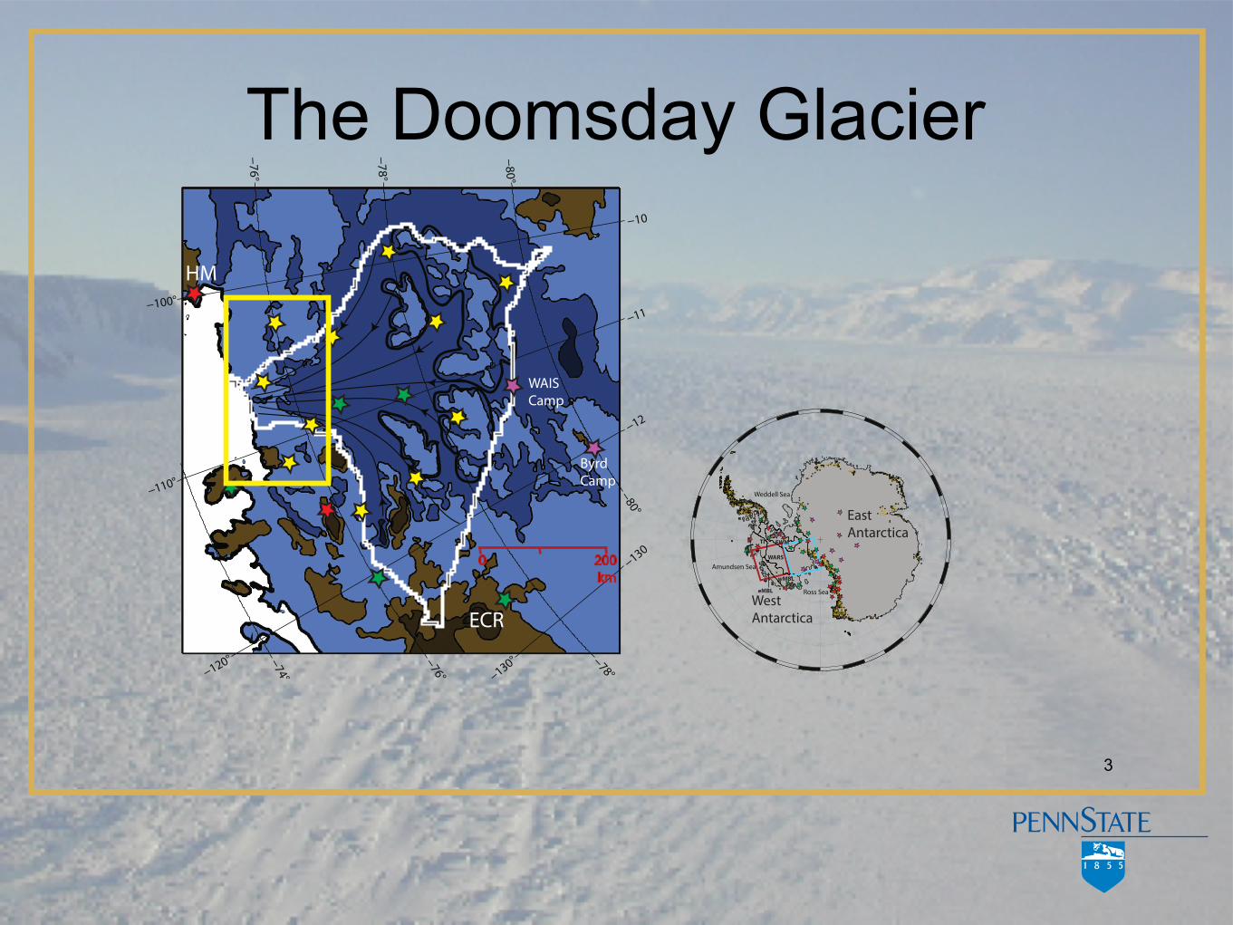
The Doomsday Glacier

3

EastAntarctica

WestAntarctica

eMBL

WARS

TI EWM

AP

wMBL

ECR

HM

0 200 km

WAISCamp

ByrdCamp

4

• The basal boundary condition is critical• Thwaites rate of retreat depends on the

sliding law…• …already unstable (Mouginot et al., 2015,

Joughin et al., 2015, Parizek et al., 2014)• …to stable for millennia (Parizek, ibid)

• Thwaites rate of retreat depends on high-resolution topography.

5

Imaging the bed of Thwaites

• Siple Coast ice streams well lubricated –flapping of butterfly wings control them –tides, small changes in till properties, etc.

• Large outlet glaciers are “narrow”: steep and deep sides; sides matter most

• Thwaites bed may dominate

6

All the greats…• H Rothlisberger, G de Q Robin, GKC Clarke,

DR MacAyeal, CR Bentley, H Kohnen, K Echelmeyer

7

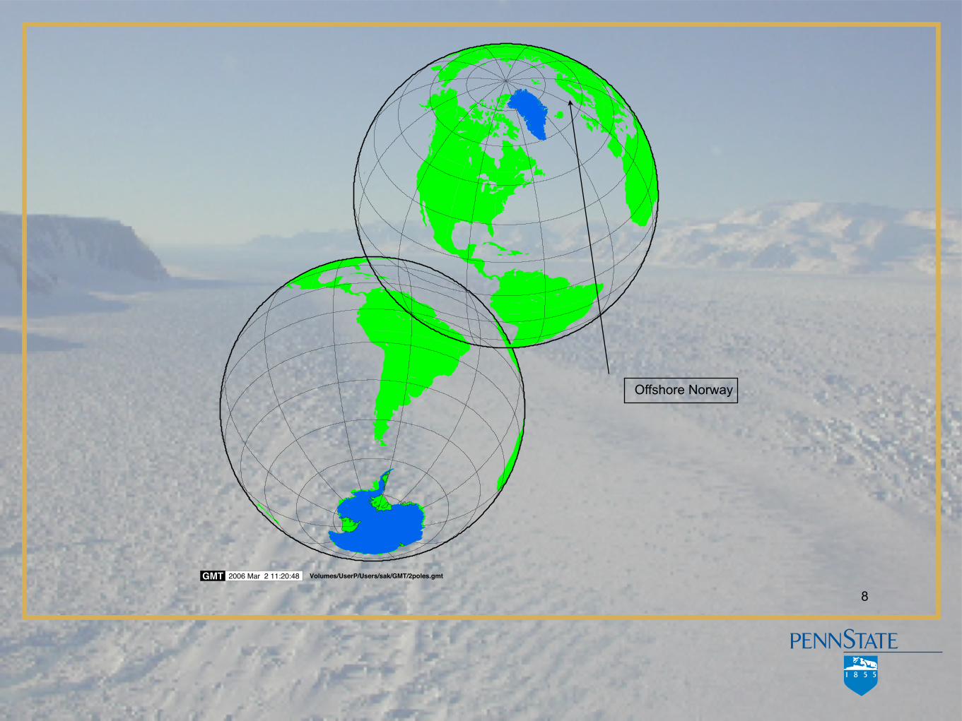
8GMT 2006 Mar 2 11:20:48 Volumes/UserP/Users/sak/GMT/2poles.gmt

Offshore Norway

9

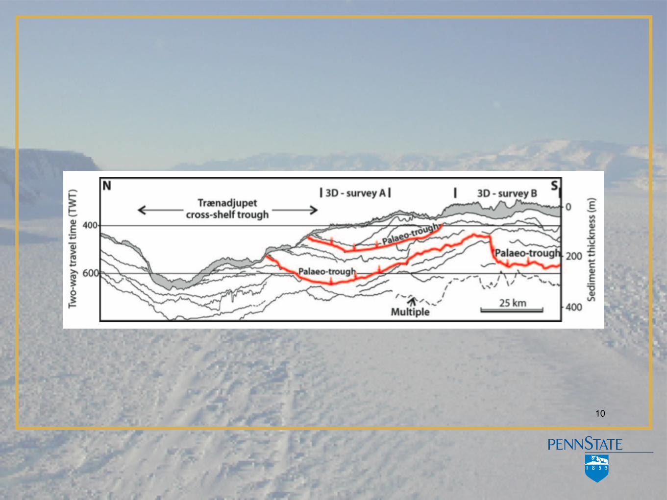
GEOLOGY, April 2006 315

Figure 3. Streamlined sedimentary bedforms produced beneath paleo–ice streams on mid-Norwegian continental shelf. A: Buried surface ~100 m deep within upper Naust Formation(three-dimensional [3D] seismic block NLGS-95). B: ~200 m deep within upper Naust For-mation (3D seismic block NNE-2000). C: Late Weichselian sediments at modern seafloor ofTraenadjupet (3D seismic block ST-9404). D: Seafloor of Vestfjorden (EM1002 swath bathym-etry). E: Map of changing ice-stream flow directions inferred from orientation of streamlinedbedforms on mid-Norwegian shelf (located in Fig. 1A). Red lines are Elsterian–Saalian andwhite lines are Weichselian ice-stream flow directions, respectively. TS—TraenadjupetSlide,NS—Nyk Slide. Locations of surfaces in A–D are shown in E (labeled a–d), together withseismic line from Figure 2 (labeled N-S). Black boxes locate two 3D seismic blocks.

recently as 10–15 k.y. ago (Shipp et al., 1999;O Cofaigh et al., 2002; Ottesen et al., 2005a,2005b). They have been used to define the dis-tribution of ice streams along the entire 2500-km-long western margin of the Scandinavian-Svalbard ice sheet at the last glacial maximum!18 k.y. ago (Ottesen et al., 2005a).

We have used megascale glacial lineations(Clark, 1993) to define the locations and di-rections of ice-stream flow on the mid-Norwegian shelf over the past 300 k.y. Seis-mic reflectors, representing former glacierbeds now buried hundreds of meters below themodern seafloor, have been identified andmapped (Figs. 3A–3B). These reflectors revealdetailed patterns of streamlined bedforms,identical in form to those from the latestWeichselian glaciation (Figs. 3C–3D). Thechanging pattern of ice flow inferred from theorientations of these sets of bedforms isshown in Figure 3E. During the Elsterian andSaalian glacial periods ice flowed southwestfrom the deep trough of Vestfjorden, acrosswhat is now Traenabanken, and into theSkjoldryggen area (Figs. 3A–3B). However,the present seafloor of Traenadjupet and Vest-fjorden shows lineations extending downVestfjorden and then turning almost 90" intoTraenadjupet, where they extend !100 km tothe shelf edge (Ottesen et al., 2005a, 2005b)(Figs. 3C–3D). A major switch in ice-streamflow direction has therefore taken place (Fig.3E).

The change in ice flow direction after theSaalian glaciation is supported by the growthof a major depositional center of at least 1500km3 at the mouth of Traenadjupet during theWeichselian period (Fig. 1D). The depocenteris composed mainly of stacked glacigenic de-bris flows, but !900 km3 has been removedby the 4-k.y.-old Traenadjupet Slide (Fig. 1D)(Henriksen and Vorren, 1996; Laberg et al.,2002) and an unknown but probably muchsmaller volume from the older Nyk Slide (Fig.3E) (Lindberg et al., 2004). Rapid delivery ofsediments from fast-flowing ice is required inorder to build a depocenter of these dimen-sions (Dowdeswell and Siegert, 1999). In ad-dition, seismic data show that these glacier-derived deposits are underlain by acousticallylayered fine-grained sediments deposited overthe Elsterian and Saalian periods (Dahlgren etal., 2002; Bryn et al., 2005). This materialis interpreted as a contourite, deposited bynorthward-flowing ocean currents in the ab-sence of large-scale sediment delivery fromglaciers to the slope beyond the present Traen-adjupet. The switch in flow direction is furthersupported through evidence of deep erosionby the Weichselian ice stream, which truncat-ed earlier seismic reflectors and units at theflanks and base of Traenadjupet (Fig. 2). We

calculate that the ice stream, !100 km long,50 km wide, and having an erosive depth of0.15 km, evacuated at least 750 km3 of sedi-ment from this cross-shelf trough.

LARGE-SCALE ICE-STREAMSWITCHING

This evidence demonstrates large-scaleswitching of ice-stream flow within a major

ice sheet from one glaciation to the next. Thechange in flow direction may have taken placebecause of continuing buildup of glacier-derived sediments on the mid-Norwegian con-tinental shelf and the filling of the availableaccommodation space. When Weichselian icebegan to flow down Vestfjorden, its easiestpath to the shelf edge was no longer acrossTraenabanken, supplying ice and debris to the

Ottesen et al., 2005; Dowdeswell et al., 2006

10

11

GEOLOGY, April 2006 315

Figure 3. Streamlined sedimentary bedforms produced beneath paleo–ice streams on mid-Norwegian continental shelf. A: Buried surface ~100 m deep within upper Naust Formation(three-dimensional [3D] seismic block NLGS-95). B: ~200 m deep within upper Naust For-mation (3D seismic block NNE-2000). C: Late Weichselian sediments at modern seafloor ofTraenadjupet (3D seismic block ST-9404). D: Seafloor of Vestfjorden (EM1002 swath bathym-etry). E: Map of changing ice-stream flow directions inferred from orientation of streamlinedbedforms on mid-Norwegian shelf (located in Fig. 1A). Red lines are Elsterian–Saalian andwhite lines are Weichselian ice-stream flow directions, respectively. TS—TraenadjupetSlide,NS—Nyk Slide. Locations of surfaces in A–D are shown in E (labeled a–d), together withseismic line from Figure 2 (labeled N-S). Black boxes locate two 3D seismic blocks.

recently as 10–15 k.y. ago (Shipp et al., 1999;O Cofaigh et al., 2002; Ottesen et al., 2005a,2005b). They have been used to define the dis-tribution of ice streams along the entire 2500-km-long western margin of the Scandinavian-Svalbard ice sheet at the last glacial maximum!18 k.y. ago (Ottesen et al., 2005a).

We have used megascale glacial lineations(Clark, 1993) to define the locations and di-rections of ice-stream flow on the mid-Norwegian shelf over the past 300 k.y. Seis-mic reflectors, representing former glacierbeds now buried hundreds of meters below themodern seafloor, have been identified andmapped (Figs. 3A–3B). These reflectors revealdetailed patterns of streamlined bedforms,identical in form to those from the latestWeichselian glaciation (Figs. 3C–3D). Thechanging pattern of ice flow inferred from theorientations of these sets of bedforms isshown in Figure 3E. During the Elsterian andSaalian glacial periods ice flowed southwestfrom the deep trough of Vestfjorden, acrosswhat is now Traenabanken, and into theSkjoldryggen area (Figs. 3A–3B). However,the present seafloor of Traenadjupet and Vest-fjorden shows lineations extending downVestfjorden and then turning almost 90" intoTraenadjupet, where they extend !100 km tothe shelf edge (Ottesen et al., 2005a, 2005b)(Figs. 3C–3D). A major switch in ice-streamflow direction has therefore taken place (Fig.3E).

The change in ice flow direction after theSaalian glaciation is supported by the growthof a major depositional center of at least 1500km3 at the mouth of Traenadjupet during theWeichselian period (Fig. 1D). The depocenteris composed mainly of stacked glacigenic de-bris flows, but !900 km3 has been removedby the 4-k.y.-old Traenadjupet Slide (Fig. 1D)(Henriksen and Vorren, 1996; Laberg et al.,2002) and an unknown but probably muchsmaller volume from the older Nyk Slide (Fig.3E) (Lindberg et al., 2004). Rapid delivery ofsediments from fast-flowing ice is required inorder to build a depocenter of these dimen-sions (Dowdeswell and Siegert, 1999). In ad-dition, seismic data show that these glacier-derived deposits are underlain by acousticallylayered fine-grained sediments deposited overthe Elsterian and Saalian periods (Dahlgren etal., 2002; Bryn et al., 2005). This materialis interpreted as a contourite, deposited bynorthward-flowing ocean currents in the ab-sence of large-scale sediment delivery fromglaciers to the slope beyond the present Traen-adjupet. The switch in flow direction is furthersupported through evidence of deep erosionby the Weichselian ice stream, which truncat-ed earlier seismic reflectors and units at theflanks and base of Traenadjupet (Fig. 2). We

calculate that the ice stream, !100 km long,50 km wide, and having an erosive depth of0.15 km, evacuated at least 750 km3 of sedi-ment from this cross-shelf trough.

LARGE-SCALE ICE-STREAMSWITCHING

This evidence demonstrates large-scaleswitching of ice-stream flow within a major

ice sheet from one glaciation to the next. Thechange in flow direction may have taken placebecause of continuing buildup of glacier-derived sediments on the mid-Norwegian con-tinental shelf and the filling of the availableaccommodation space. When Weichselian icebegan to flow down Vestfjorden, its easiestpath to the shelf edge was no longer acrossTraenabanken, supplying ice and debris to the

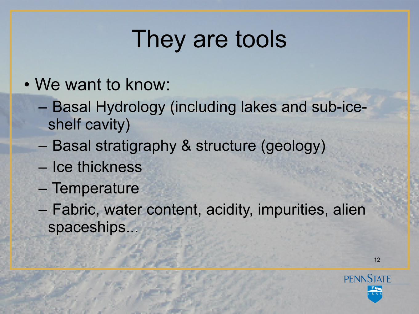
They are tools

• We want to know: – Basal Hydrology (including lakes and sub-ice-

shelf cavity) – Basal stratigraphy & structure (geology) – Ice thickness – Temperature – Fabric, water content, acidity, impurities, alien

spaceships...

12

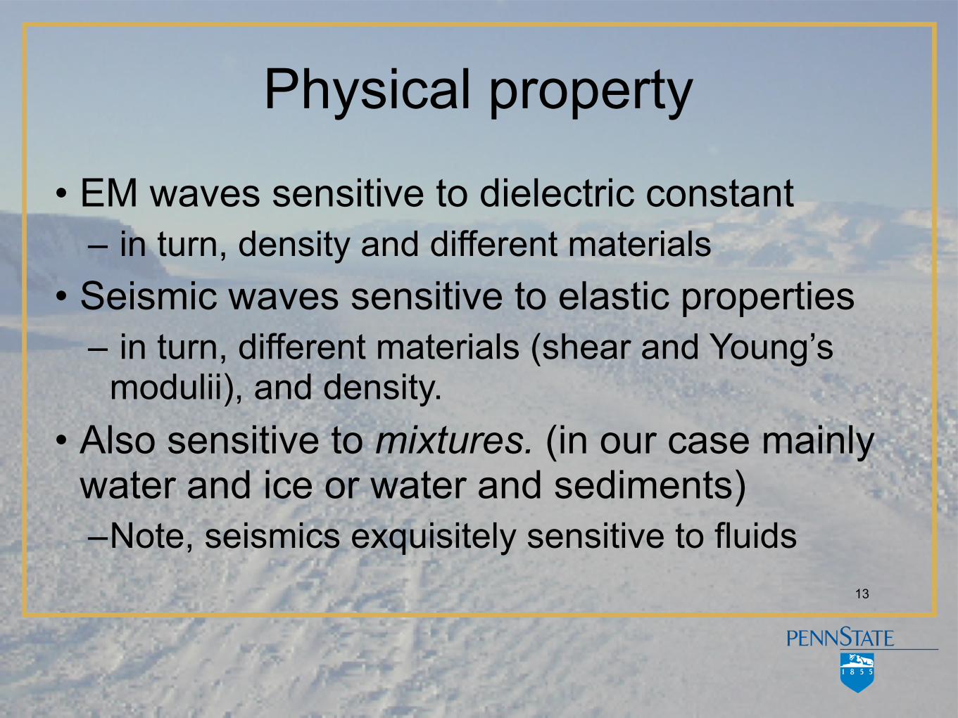
Physical property

13

• EM waves sensitive to dielectric constant – in turn, density and different materials

• Seismic waves sensitive to elastic properties – in turn, different materials (shear and Young’s

modulii), and density. • Also sensitive to mixtures. (in our case mainly

water and ice or water and sediments) –Note, seismics exquisitely sensitive to fluids

Typical numbers...

• Radar frequencies: 1 to 400 MHz –Wavelengths: 180m to 1/2 m

• Seismic frequencies: 20 Hz to 400 Hz –Wavelengths: 200 m to 10 m

• for seismics BW ~ center frequency • for radar, bandwidth often << center frequency

14

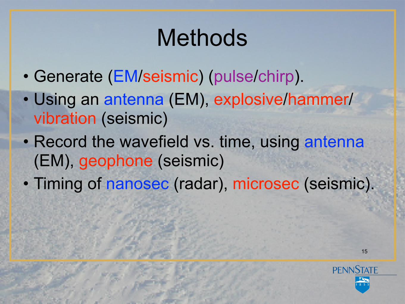
Methods• Generate (EM/seismic) (pulse/chirp). • Using an antenna (EM), explosive/hammer/

vibration (seismic) • Record the wavefield vs. time, using antenna

(EM), geophone (seismic) • Timing of nanosec (radar), microsec (seismic).

15

Key differences

• EM waves can be generated/recorded in air or on ice.

• Seismic waves must be generated/recorded on ice. – Contrast in permittivity vs. contrast in rho x V

• Timing requirement allows seismic source/receiver to be physically separate;harder to separate EM source/receiver antennas. 16

Typical reflectivities...

17

Radar SeismicSeawater -1 -8Freshwater -3 -8Till -6 -27Rock -30 -9Internal Fabric -30 or less -33

Power (dB)

Absorption 20 dB/km Strong fn of T

2 dB/km Weak fn of T

• Radar –Monostatic is most common –few to 10s of m postings (reflection points) –side looking through-ice SAR on the horizon

• Seismic –Bistatic is most common –few to 10s of m postings –along-track SAR common (“migration”) –3D uncommon but on the horizon

Geometries

18

Production

• Radar –100 to 1000s of km per day

• Seismic –few km per day

19

Key Differences (2)

• Subglacial penetration possible with seismics –Radar absorption large in water/rock (plus poor

injection of energy) • Bistatic geometry allows for velocity

tomography. • Bistatic geometry allows us to exploit changes

in reflectivity as fn of angle of incidence. – At non-normal incidence, phase conversions (P to

SV) steal energy... water = large ∆ Vs 20

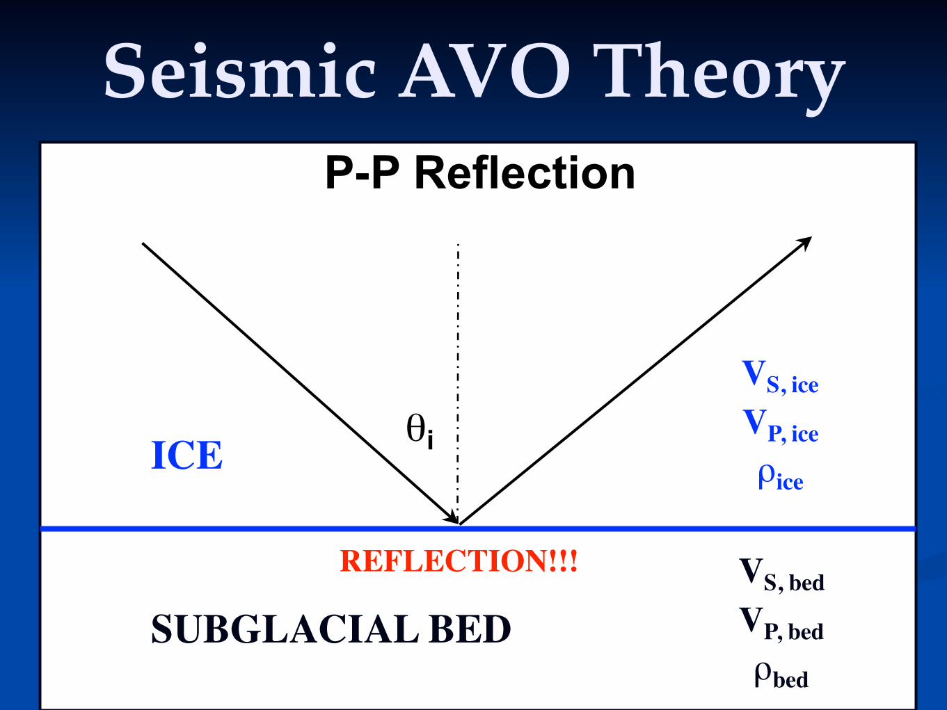
Seismic AVO Theory

P-P Reflection

θiICE

SUBGLACIAL BED

VS, ice

VP, iceρice

VS, bed

VP, bedρbed

REFLECTION!!!

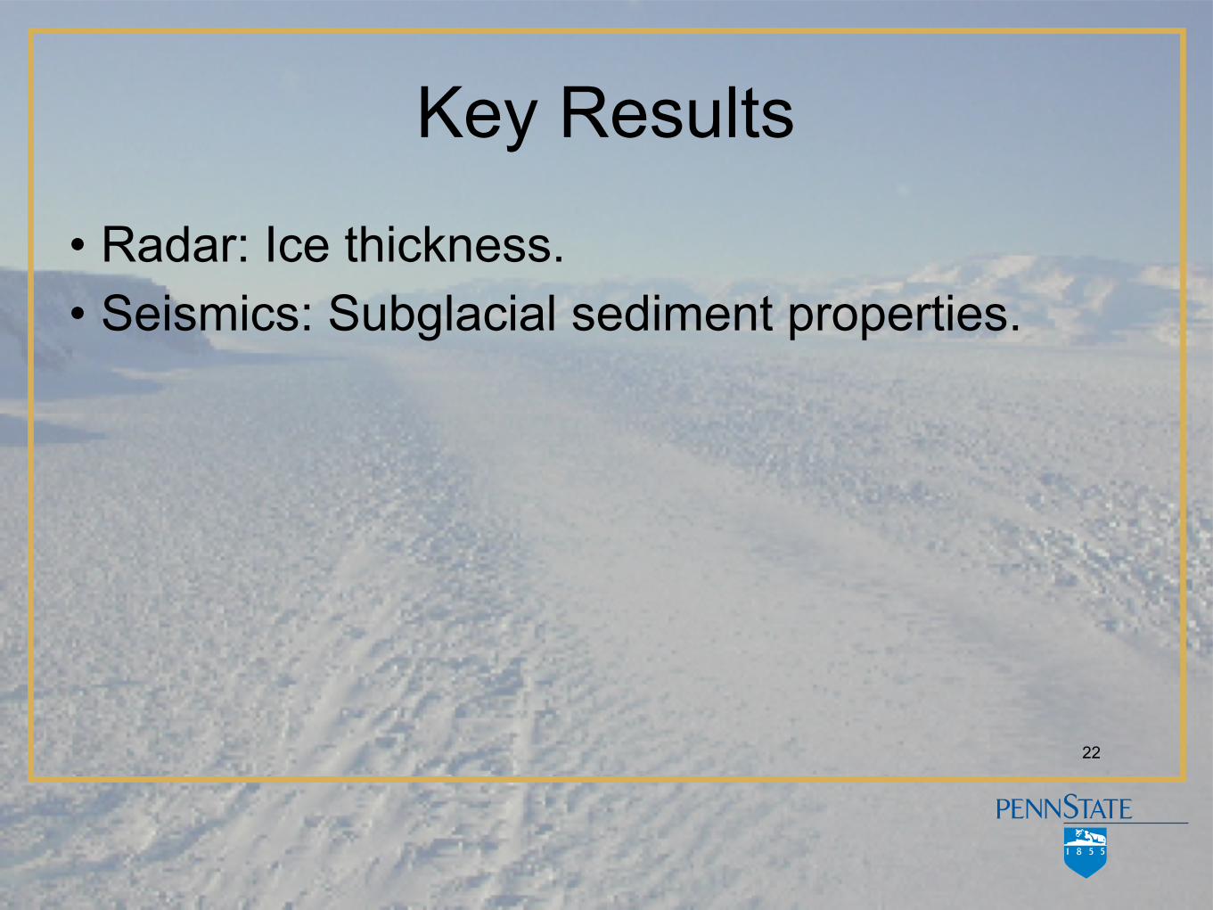
Key Results

• Radar: Ice thickness. • Seismics: Subglacial sediment properties.

22

23GMT 2006 Mar 2 11:20:48 Volumes/UserP/Users/sak/GMT/2poles.gmt

South Pole

Radar from the S. Pole

South Pole Lake region

UTIG Radar Data

5 km

100 m

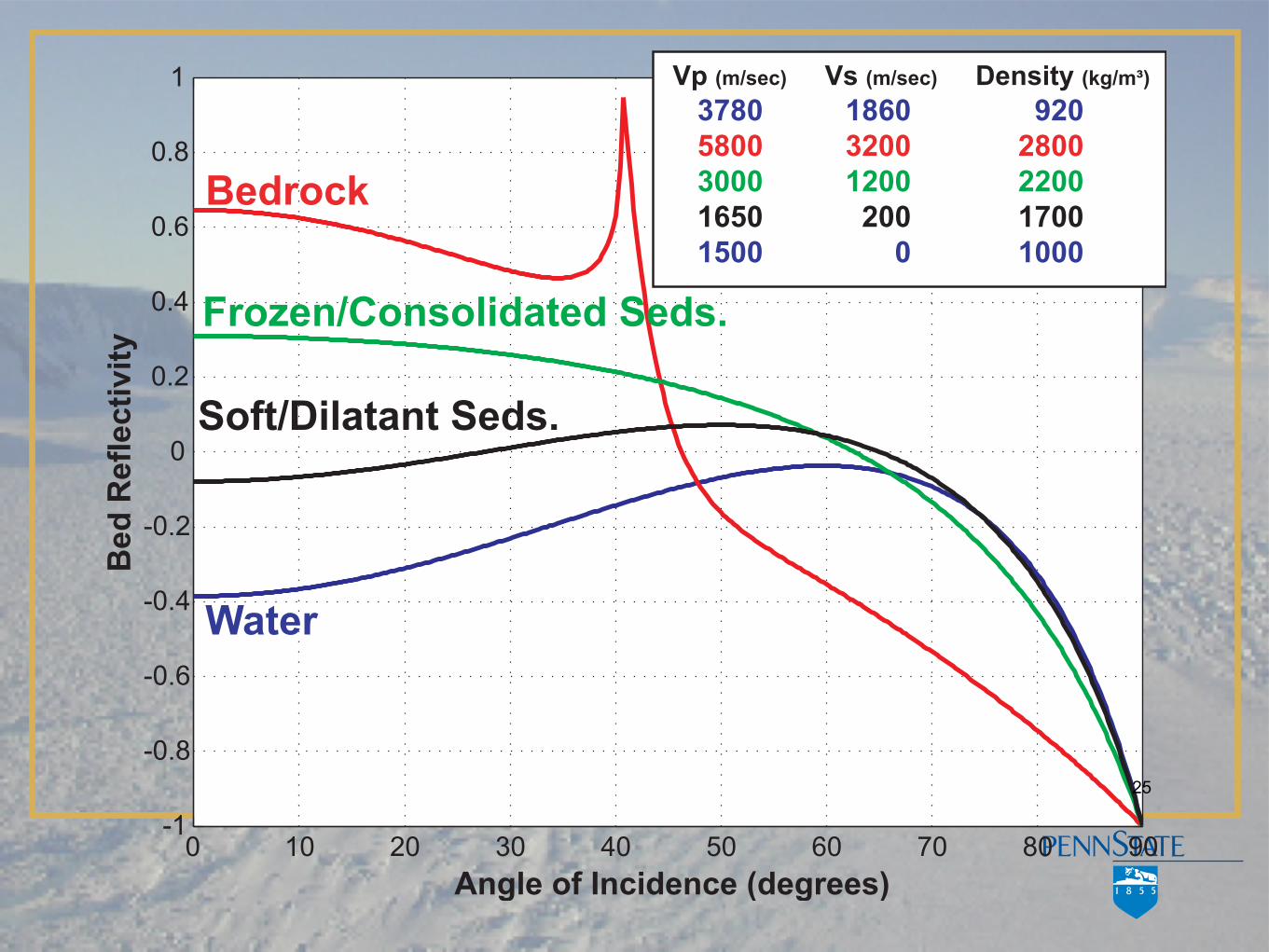
0 10 20 30 40 50 60 70 80 90-1

-0.8

-0.6

-0.4

-0.2

0

0.2

0.4

0.6

0.8

1

Angle of Incidence (degrees)

Be

d R

efl

ec

tiv

ity

Bedrock

Water

Frozen/Consolidated Seds.

Soft/Dilatant Seds.

Vp (m/sec) Vs (m/sec) Density (kg/m³)

3780 1860 920

5800 3200 2800

3000 1200 2200

1650 200 1700

1500 0 1000

25

Ice over Water

They are tools ... which one?

• We want to know: – Basal Hydrology (including lakes and sub-ice-

shelf cavity) – Basal stratigraphy & structure (geology) – Ice thickness – Temperature – Fabric, water content, acidity, impurities, alien

spaceships...

27

They are tools... which one?– Basal Hydrology

• Seismics & radar (problematic) – Basal stratigraphy & structure (geology)

• Seismics (maybe radar for some cases + bedforms) – Temperature & Water content

• Combined radar and seismics (Navarro, Benjumea)

28

They are tools... which one?– Ice thickness, isochrons

• Radar.. except when it doesn’t work – Fabric

• Seismics, polarimetric radar

• Joint inversion of seismic and radar data is the next frontier. –Example: is an internal reflector an impurity or

density contrast? –Example: can we invert for temperature from

velocity and attenuation of both? –Example: Basal roughness

29