Seismic Waves in Laterally Inhomogeneous...
25
Geophys J. R. usfr. SOC. (1972) 27. 301-325. Seismic Waves in Laterally Inhomogeneous Media B. L. N. Kennett (Received 1971 September 24) Summary A new perturbation technique is presented for the approximate solution of problems involving slight lateral inhomogeneities, or moderate in- homogeneities of small lateral extent, in elastic media. The method, based on an integral equation formulation and Born-type expansion in the wavenumber domain, is an extension of the usual matrix methods for multilayered elastic media. It is thus particularly suitable for problems concerning inclusions in multilayered half spaces. As an example of this method calculations are made of the scattering effects produced by near-surface inclusions in simple half-space models. It is found that at low frequencies forward and backward scattering into surface waves are of comparable importance, but as the frequency of the incident waves increases the forward scattering tends to dominate. 1. Introduction The results of many recent studies suggest that as well as the widely recognized lateral variations in crustal velocities, there are lateral variations of up to 10 per cent in P wave velocities in the Continental Upper Mantle see James & Steinhart (1966), Herrin ( 1969). Previous work on inhomogeneous elastic media in the presence of a horizontal free surface has concentrated on problems involving only vertical inhomogeneities; a number of specific models have been treated (see for example Ewing, Jardetsky & Press (1957). Horizontally layered structures have been tackled using matrix methods (Thompson 1950; Haskell 1953), and recently the more general method of ' propa- gator ' matrices has been introduced by Gilbert & Backus (1966). Very little work has however been done on problems involving lateral as well as vertical inhomogeneity, despite their geophysical importance. A generalized ray treatment of the propagation of surface waves in a half space with lateral and vertical inhomogeneity has been given by Babich & Molotkov (1966) for Love waves and Mukhina & Molotkov (1967) for Rayleigh waves. Bhattacharya (1970) has considered Love wave dispersion in an inhomogeneous layer, with linear dependence of shear velocity and shear modulus on horizontal distance, overlying a homogeneous half space. A more general method for surface wave dispersion is that of Zharkov & Osnach (1970) who have developed a perturbation method to examine the dispersive effect of media with slight lateral and vertical inhomogeneity superimposed upon a horizontally multilayered structure, the lateral variations being supposed to be of limited extent. The above work has been confined to the treatment of surface waves in the presence of a lateral variation of properties. We consider here a perturbation scheme for calculating the scattering effects of 301
Transcript of Seismic Waves in Laterally Inhomogeneous...

Geophys J . R . usfr. SOC. (1972) 27. 301-325.
Seismic Waves in Laterally Inhomogeneous Media
B. L. N. Kennett
(Received 1971 September 24)
Summary
A new perturbation technique is presented for the approximate solution of problems involving slight lateral inhomogeneities, or moderate in- homogeneities of small lateral extent, in elastic media. The method, based on an integral equation formulation and Born-type expansion in the wavenumber domain, is an extension of the usual matrix methods for multilayered elastic media. It is thus particularly suitable for problems concerning inclusions in multilayered half spaces.
As an example of this method calculations are made of the scattering effects produced by near-surface inclusions in simple half-space models. It is found that at low frequencies forward and backward scattering into surface waves are of comparable importance, but as the frequency of the incident waves increases the forward scattering tends to dominate.
1. Introduction
The results of many recent studies suggest that as well as the widely recognized lateral variations in crustal velocities, there are lateral variations of up to 10 per cent in P wave velocities in the Continental Upper Mantle see James & Steinhart (1966), Herrin ( 1969).
Previous work on inhomogeneous elastic media in the presence of a horizontal free surface has concentrated on problems involving only vertical inhomogeneities; a number of specific models have been treated (see for example Ewing, Jardetsky & Press (1957). Horizontally layered structures have been tackled using matrix methods (Thompson 1950; Haskell 1953), and recently the more general method of ' propa- gator ' matrices has been introduced by Gilbert & Backus (1966). Very little work has however been done on problems involving lateral as well as vertical inhomogeneity, despite their geophysical importance.
A generalized ray treatment of the propagation of surface waves in a half space with lateral and vertical inhomogeneity has been given by Babich & Molotkov (1966) for Love waves and Mukhina & Molotkov (1967) for Rayleigh waves. Bhattacharya (1970) has considered Love wave dispersion in an inhomogeneous layer, with linear dependence of shear velocity and shear modulus on horizontal distance, overlying a homogeneous half space. A more general method for surface wave dispersion is that of Zharkov & Osnach (1970) who have developed a perturbation method to examine the dispersive effect of media with slight lateral and vertical inhomogeneity superimposed upon a horizontally multilayered structure, the lateral variations being supposed to be of limited extent. The above work has been confined to the treatment of surface waves in the presence of a lateral variation of properties.
We consider here a perturbation scheme for calculating the scattering effects of 301

302 B. L. N. Kennett
lateral inhomogeneities in multilayered elastic media which may be used for body waves or surface waves. This technique, based on an integral equation formulation and a Born-type approximation, is suitable for slight slowly varying lateral inhomo- geneities or moderate inhomogeneities of small lateral extent. The approach may be regarded as an alternative to that of Herrera & Ma1 (1965) and has the advantage that it is an extension of the usual methods for problems of layered media.
The method we use differs also from that adopted by Hudson & Knopoff (1966) by working in the wave number domain, and is not so dependent on a large separation between the region of inhomogeneity and the point of observation.
2. Basic equations
We consider an isotropic medium and look at two-dimensional problems, where all stresses and displacements are independent of the co-ordinate y. A harmonic time dependence of the form exp (-iot) will be assumed throughout though it will not usually be explicitly represented.
For a general two-dimensionally inhomogeneous medium, the equations of motion and the stress-strain relations may be combined and rearranged to a form where derivatives with respect to z appear only on the left-hand sides of the equations:
and
where (u, u, w) is the displacement vector, zt, the stress tensor, A, p are the Lam6 parameters and p the density of the medium.
We see that the equations (2.1)-(2.6) divide into two distinct groups
(a) Equations (2.1)-(2.4) associated with P and SV wave propagation; and
(b) Equations (2.5)-(2.6) associated with SH wave propagation.
Introducing the compressional velocity a, and the shear velocity p, given by

Seismic waves in laterally inhomogeneous media
the sets of equations above can be written in the form
303
This arrangement of the equations is particularly convenient since the stress- displacement column vectors in (2 .8 ) and (2 .9 ) are both continuous across any interface perpendicular to the z-axis, i.e. for any interface in horizontal stratification.
We will assume that the inhomogeneities in the medium may be represented by a lateral variation superimposed on a vertical inhomogeneity, i.e.
For future convenience we will introduce the following notation
(2.10)
I (2.11)
Where the quantities a,(x, z) are measures of the local departures of the elastic moduli I, p and density p from their values for a laterally homogeneous medium.
With this form of inhomogeneity we may write the equations (2 .8 ) and (2 .9 ) in the form
(2.12) a aZ - B(x,z) = Ao(z)B(x,z)+A1(x,z)B(x,~)
where A&) is the operator matrix corresponding to a laterally homogeneous medium, with density po(z), velocities ao(z), Bo(z)-and is independent of the co-ordinate x ; the effects of the lateral inhomogeneity are described by the operator matrix A, (x , z), which depends on the ' inhomogeneity measures ' a,(x, z) introduced above.

304 B. L. N. Kennett
For the P-SV wave case: the stress-displacement vector is
Bp = col [u, w, 7x2, 4 and Ao(z) has the form
I 0 -8, ( P o B0'Y-l
- P o w2 - a x
where oo = Po/ao, vo = 4p0 Po2(l -no2) and the matrix introduced by the lateral inhomogeneity is
f 0
For the SH wave case: the stress-displacement vector is simply
B,, = COI [u, T,.,] and
0 (2 .15 )
0 - Po Po' a,, - P o w2
0 - (a, a6) a, - a,, - a , w2 o A , ( x , z ) =
Taking the Fourier transform of equation (2 .12) with respect to x and writing rr:
Sk [u(x, z , w ) ] = i ( k , z , w ) = u(x, z , w ) exp (- ikx) dx (2 .16 ) s we obtain
i C ( k , t , z ) B(t ,z)&, (2 .17) a - B ( k , z ) = A0(k,z) B(k , z )+ - az 2n
-7?
where in the P-SV case
(2 .18 )
0 -ik (Po P o 2 ) - ' 0 (2aO2-I)ik 0 0 (Po a0')-
0 - P o w2 - ik 0 " o k 2 - p 0 w 2 0 0 (2aO2 - 1) ik
and in the SH case
(2.19)
Seismic waves in laterally inhomogeneous media 305
which are the usual coefficient matrices for a laterally homogeneous medium of density po and velocities a0, Po encountered in the theory of elastic propagator matrices.
The ' inhomogeneity ' matrices C(k, 4, z) may be calculated by using the result that the Fourier transform of a product is the convolution of the Fourier transforms.
(2.20) 1
2lr f , [ u u ] = -u * iqk)
and have the form
C,(k, 4, z )
1 0 0 a, W-t, Z ) 0 itl73(k-t,z) 0 0 M k - t , 2 )
0 -02 a , (k - ( , z) 0 0 kZ,(k-4, z) - 02a,(k - 5 , z) 0 0 ika3(k- t , z )
(2.21) and
We will assume that the quantities a,(x, z) are piecewise continuous and differentiable, so that their Fourier transforms ii,(k, z ) are defined for all k.
By this method we have been able to separate out the effects of the lateral in- homogeneity so that equation (2.17) is that for a laterally homogeneous medium modified by an additional integral term introduced by the lateral variation.
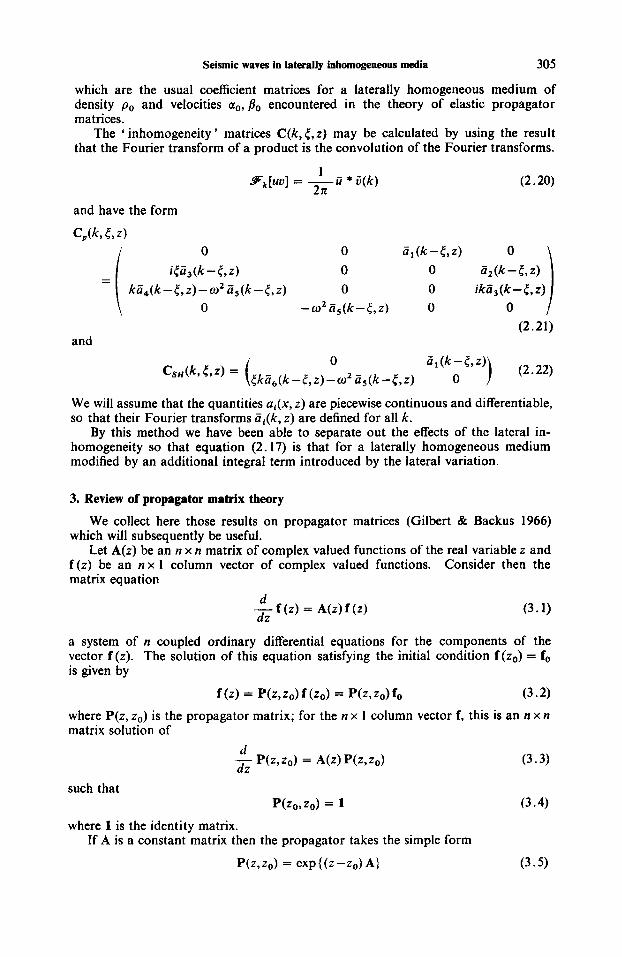
3. Review of propagator matrix theory
which will subsequently be useful.
f (z) be an n x 1 column vector of complex valued functions. matrix equation
We collect here those results on propagator matrices (Gilbert & Backus 1966)
Let A(z) be an n x n matrix of complex valued functions of the real variable z and Consider then the
(3.1) d dz - f (z) = A ( z ) f ( z )
a system of n coupled ordinary differential equations for the components of the vector f (z). The solution of this equation satisfying the initial condition f (zo) = fo is given by
(3.2) where P(z, zo) is the propagator matrix; for the n x 1 column vector f, this is an n x n matrix solution of
f(z) = P(z,zo)f(zo) = P(z,zo)fo
such that
where 1 is the identity matrix. P(Z0,ZO) = 1
If A is a constant matrix then the propagator takes the simple form
(3 .4)

306 B. L. N. Kennett
and the determinant of the propagator satisfies
det P(z,zo) = exp (1 tr A ( 0 dC] (3.6)
for all forms of A(z).
that From the definition of the propagator one may show that it is unique, and also
(3 * 7)
P-'(z,z,) = P(z0,z). (3.8)
P(Z, 0 P(C, zo) = P(z, zo), so that it bears a very simple relation to its inverse
Using the propagator matrix we may solve the inhomogeneous set of equations
d (3 * 9) dz
for given initial conditions on f. Premultiplying (3.9) by P-'(z,z0), where P(z,zo) is the propagator for the homogeneous equations, we find
- f(z) = A(z)f (z)+g(z)
d dz
P-'(z,z0) -f(z)-PP-'(z,zO)A(z)f (z) = P-'(z,zo)g(z),
so that
where we have used equation (3.8). Integrating (3.10) with respect to z and using the relation (3.7) we obtain
z
f(z) = p(z,zo)f(zo)+ J p(z,Y)g(Y)dY (3.11)
as the solution of the set of inhomogeneous equations (3.9) with initial conditions prescribed at z = zo. Thus the propagator is simply the Green's function of the equation (3.1).
20
4. Approximate treatment of sligbt lateral inhomogeneity
In this section we set up an exact integral equation for the stress-displacement field in the presence of an arbitrary ' well-behaved ' lateral inhomogeneity, and are then able to find an approximate solution for the case of a slight lateral inhomogeneity.
Consider equation (2.17)
-uJ
We may take this to be in the form of equation (3.9) by setting m
-a
and may then apply the results (3.10)-(3.11). Writing Po@, z,zo) for the propagator

Seismic waves in laterally inhomogeneous media 307
matrix for the homogeneous equation
i.e. the propagator appropriate to a laterally homogeneous medium with velocities ao, Po and density po, we then find from equation (3.14)
2 m 1 , .
20 - m
Thus the problem of a lateral inhomogeneity has been reduced to a description in terms of a two-dimensional integral equation. In (4.4) the effects of the lateral variation are still kept distinct and the first term on the right-hand side is simply that expected for a laterally homogeneous medium.
For a slight inhomogeneity in the horizontal direction, i.e. one in which
(4 * 5 )
(4 * 6)
1 SUP bl(X,Z)I Q a09
SUP I P l ( 4 Z ) l Q Po,
SUP IPl(X,Z)l Q Po,
we expect that the total stress-displacement field will have the form
B(x, z) = B0(x, Z) + B' (x, Z)
where Bo(x,z) is the field expected in the case where no lateral inhomogeneity is present, (the ' zeroth order ' field) and the scattered contribution is small, i.e.
IB'(x,z) I Q IB0(x,z)l. (4 * 7)
Then equation (4.4) can be written as
B ( k z) = Po& z, zo) w, zo)
(4.8)
and, provided we may neglect multiple scattering, we may neglect the last term on the right hand side of (4.8) (cf. Hudson & Knopoff 1966). For this approximation to be valid
I
since then the neglected term will be of the second order of small quantities. This condition together with the behaviour of the inhomogeneity measures

308 B. L. N. Kennett
ai(x, z), is sufficient to ensure that no problems arise from the high frequency behaviour of the scattered field on inverting the Fourier transform.
We will assume that the zeroth order field is composed of wave trains whose horizontal wave numbers lie within a limited band - K ~ c k < rc0. For plane SV waves travelling at an angle 8 to the z axis k = o/B sin8 and so any field of plane SV waves may be described by setting K, = w/B. Thus, using the Hadamard in- equality (Hadamard I893),
I 2n K = - ( [det{Po(k,z ,~)C(k,5,~)} l"" 1 ~ o ( 5 , ~ ) l ~ t d ~ (4.10)
:o - K O
where rn is the dimension of the column vector B(k,z), i.e. m = 4 for the P-SV case, ni = 2 for the SH case. Also for the laterally homogeneous medium
so that we have
i o - K O
since
and from equation (3.8)
det Po(k,:, y) = exp tr A 0 ( ~ ) d ( = 1, I! i as tr A, = 0 for both the coefficient matrices (2.18) and (2.19). Now
b
a
so that considering an inhomogeneous layer of thickness H
and we may satisfy the condition (4.9) if
(4.13)
(4.14)
We may note that though the elements of C(k, 5 , z ) depend on the dimensional quantities iii, det C only involves them in non-dimensional combinations. Introducing the non-dimensional forms
(4.15)
where p*, p * are averaged parameters, we may write the determinants of the ' lateral inhomogeneity ' matrices C(k, 5, z) in the form:
61 = ii, p*, 6 2 = 5 2 /A*, 6 3 = 33,
64 = i i J p * , ti, = i i , /p*, ti, = i i6 /p* ,

Seismic waves in laterally inhomogeneous media
for the P-SV case
and for the SH case
309
(4.16)
(4.17)
where we have written K~ = o / p , and 6i = 6 i ( k - t , y ) . The assumption of piecewise continuity for the b i (x , z ) ensures that no convergence problems arise at large wave- numbers.
Now f ( k - t ) < L SUP If(x)l (4.18)
Thus defining the two where L is the maximum linear extent of the function. quantities
the condition (4.14) will certainly be satisfied if for the P-SV wave case
and for the SH wave case
(4.19)
(4.20)
(4.21)
(4.22)
where L is the width of the lateral inhomogeneity. These rather stringent conditions may in fact be relaxed slightly and the approxi- mation is expected to be quite good provided that for example for P-SV waves
o H L - x 0 - b p < 1. B n
(4.23)
These conditions may be interpreted either as an upper bound on the acceptable frequencies for a specified zeroth order field; or as bounds on the range of ' incident ' wavenumbers which may be considered at a given frequency. For a region with cross-sectional area 100 km2 whose properties have a 10 per cent contrast with the surrounding matrix (shear wave speed 3.5 km s-'), this method will be suitable for considering incident waves whose periods are larger than about 5 s.
Hence for a slight lateral inhomogeneity at up to moderate frequencies we may find the scattered field contribution from
and, since the zeroth order field represents the solution for a laterally homogeneous medium
Bo(k , z ) = Po(k , z , zo ) Bo(k ,zo) (4.25)

310 B. L. N. Kennett
and thus equation (4.24) may be rewritten as
20 -xo (4.26a)
(4.26b)
Similarly we may describe a moderate inhomogeneity of small lateral or vertical extent by this first order approximation (cf. Herrera & Ma1 1965) provided that the frequency satisfies the relevant condition (4.21) or (4.22).
Examining the form of equation (4.26a) we see that the scattering effect of the lateral inhomogeneity has been introduced as the integrated result of source terms dependent on the stress-displacement field in the inhomogeneous region, i.e. each volume element in that region is acting as a radiator with source characteristics determined by the local field (cf. Hudson & Knopoff 1966).
As indicated by the conditions (4.21) and (4.22) above, this approximation will break down for a large volume of lateral inhomogeneity (i.e. H L large) since it is then no longer a good approximation to assume that the local field at each volume element is described by the zeroth order field at that point, as is implicitly assumed in (4.26a); and furthermore as the scattering volume increases multiple scattering effects become more important.
5. Effect of a lateral inhomogeneity in a single layer
Consider a horizontally layered elastic half space as shown in Fig. 1. Each layer is supposed to be isotropic and perfectly elastic though not necessarily vertically homogeneous, the nth layer being bounded above by the plane z = 2,- and below by z = z , and having density p,(z) and compressional and shear velocities a,(z), Bn(z) The layers are underlain by a homogeneous half space with density pN and velocities
We assume a lateral inhomogeneity to be concentrated in the mth layer, where the inhomogeneity may be represented as a small laterally varying component super- imposed on a vertical variation, i.e.
aN, BN*
At the free surface z = 0, the normal and tangential stresses must vanish so that
z,, = zyz = z,, = 0, (5.2)
with the result that the surface stress-displacement vectors take the form:
in the P-SV case
in the SH case Bp(k, 0) = col [ii(k, O), E(k, O ) , O,O],
B,,(k, 0) = col [ij(k, O), 01.
(5.3)

(I)
31 1
a, (Z).B, (Z).p,(z)
Fig. 1. Layered half space.
The scattered stress-displacement vectors (due to the lateral inhomogeneity) on the two sides of the mth layer will be connected by the first order approximation
B' (k,zm- 1) = Pmo(k, z m - 1, z m ) B' (kszm)
- 1 7 Pmo(k,zm- 1, y ) cm(k, 5, y ) go(<, y) dtdys (5.4) zm-1 -It0
28
where we have used (4.26a) and Pmo(k, z, zo) is the propagator matrix corresponding to a laterally homogeneous layer with properties amo(z), pm0(z), pmo(z); provided the frequency satisfies the relevant condition (4.21) or (4.22). The character of the scattered field will thus be dependent on the assumed zeroth order field.
In the laterally homogeneous layers we may use the conventional propagator theory so that the scattered displacement field at the free surface is related to that at the top of the inhomogeneity by
where the resultant propagator matrix is the product of the propagator matrices for the m- 1 intervening layers:
since the vector B is continuous across horizontal interfaces. For homogeneous layers Pjo(k,z, ,z ,+l) is just the Haskell layer matrix for the
jth layer. Similarly, the scattered field at the bottom of the mth layer is related to that at the half-space interface z = z N - by

312 B. L. N. Kennett
Thus from (5.4), using the relation (3.10)
B' (k, 0) = Q(k, 0, zN- 1) B' (k, zN - 1 )
- 7 Q(k,O,zrn-,)P,,(k,zrn-,,y)Crn(k,r,y) B 0 ( t , Y ) d 5 d y * ( 5 . 8 ) 271 = , - I -KO
In the homogeneous half space we anticipate that the scattered field should consist of only outgoing or evanescent waves; this places a restriction on the form of B'(k, zN - ,) and enables (5.8) to be solved for either the surface scattered field or the radiation into the half space.
For the SH case the half-space propagator has the form
and in z > zN-,
In order that the stress-displacement field should correspond to outgoing or evanescent waves we must require only terms of the form exp (- qN(k)(z -zN- ,)) to appear in B(k,z); this implies that the interface value of B must have the form
(5.11)
where c(k) is a function of wave number alone.
make the transformation to normal coordinates For P-SV waves in the homogeneous half space, following Dunkin (1965) we
B(k,zN- ,) = TN(k) G(k,z), z > zN-, (5.12)
where the vector G is given by
and &+, $ N + ; 4N- , $N- are the incoming and outgoing parts of the elastodynamic potentials for the half space, i.e. the parts with exponential dependence
pectively. Here we have defined exp(cN(z-zN-I)), exp(vN(Z-ZN- 1)); exP(-cN(z-zN- 1))~ exp(-?N(z-zN-l)) res-
= ( k z - ~ 2 / a N 2 ) * , lkl > lw/aNl
= (02/aN2-k2)*, (kl < l o / a N I (5.14)
For outgoing or evanescent waves in the half space we require 4N+,$N+ to vanish,

Seismic waves in laterally inhomogeneous media
and thus the interface value of B takes the form
B ( k , z N - 1) = T N ( k ) cO1 lo, O, c1 (k) , c2(k)1,
where the matrix T N ( k ) is
ik
313
(5.15)
and xN = (2k2 - 0 2 / B N 2 ) . Consider now equation ( 5 . 8 ) and write
R = Q(k, 0 - z ~ - 1) T N ( ~ ) , which we partition into second order submatrices as
(5.17)
(5.18)
Defining also a ' scattering vector '
Zm- 1 - K O
equation ( 5 . 8 ) becomes
B'(k,O) = R(k) B'(k,ZN-l)-S(k) (5.19)
and so we find that the radiation into the lower half space is determined by
and thus the surface scattered field is
Thus writing R,,' for the transpose of the cofactor matrix of R,,
(5 .20)
(5.21)
(5.22)
where det Rz2 is the secular function for the layered half space. Inverting the Fourier transform, the surface displacements have the form
m
[ w l ( x , O ) ] u1 (x, 0) = %- 1 1 det K,, ( R 1 2 R 2 2 t [2] -detR2,[::])dk(5.23) - m
and the modal contributions for propagating surface modes and leaking modes arise from polar residues at the roots of the secular function.
For the SH case, setting
(5 .24)

314 B. L. N. Kennett
and using the form of the interface stress-displacement vector B(k,z,- (5.1 l), equation (5.8) becomes
given by
and thus the scattered displacement at the free surface is
(5.25)
(5 .26)
which may similarly be Fourier inverted, with modal contributions arising from the poles at the roots of the denominator, i.e. where
q Z l - p N q N q 2 2 O . (5.27)
To the first order approximation used above the scattering effects due to spatially separated inhomogeneities are independent; so that if there are lateral inhomogeneities in two or more layers the scattering effects may be calculated separately and then summed-provided the condition (4.7) is satisfied by the total scattered field
IBkdx, z>l 6 IBo(x,z)I (5.28)
and the frequency satisfies the relevant condition (4.21) or (4.22) for each of the inhomogeneities. In reality, of course, multiple scattering effects will occur with coupling between inhomogeneities, but these will be sufficiently small to be neglected provided that the separations are large. However, volume limitations on the validity of the first order approximation would become important if a particular lateral inhomogeneity extended through a number of vertical layers.
In the next two sections we shall discuss examples illustrating our approximate method using equations (5.22) and (5.26) for the P-SV and SH cases respectively.
6. A region of lateral inhomogeneity in a homogeneous half space
We consider here the scattering of an elastic wave incident upon an inclusion, near the surface of the half space, whose properties differ slightly from those of the half space. Using the approach of Section 5 we may describe the problem in terms of a single layer of depth hy in which the density and velocities are given by
where p1 6 po, u1 6 ao, B1 6 Bo, overlying a uniform half space with density po and elastic wave speeds ao, Po and where h is the maximum depth of the inclusion.
We will assume that the zeroth order field consists of the incident and reflected wave field due to an incident plane P or SV wave or else is a Rayleigh surface wave, and that its x-dependence may thus be represented in the form exp (iko x) (k, > 0), with the result that
E0(tY Y ) = B0(k0, Y ) S(t -ko). (6.2)
W) = To(k), (6.3)
Taking the top of the inclusion to be at the free surface we have from (5.17)
and det R,,(k) = po2 A(k) = ~02{(2k2-02/B02)2-4k2 Co(k)qo(k)} (6.4)
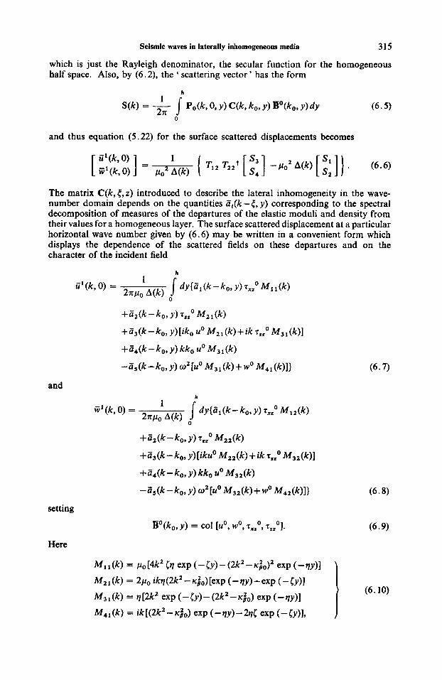
Seismic waves in laterally inhomogeneous media 315
which is just the Rayleigh denominator, the secular function for the homogeneous half space. Also, by (6 .2 ) , the ' scattering vector ' has the form
and thus equation (5 .22 ) for the surface scattered displacements becomes
The matrix C(k, t, z) introduced to describe the lateral inhomogeneity in the wave- number domain depends on the quantities Z,(k -(, y ) corresponding to the spectral decomposition of measures of the departures of the elastic moduli and density from their values for a homogeneous layer. The surface scattered displacement at a particular horizontal wave number given by (6.6) may be written in a convenient form which displays the dependence of the scattered fields on these departures and on the character of the incident field
and
setting
Here
no(/?,, y ) = col [UO, wo, Tx2O, T,,O].

316
and
B. L. N. Kennett
For an incidenr SV wave
Thus we may find the scattered field once the zeroth field is determined, for frequencies such that the conditions (4.2 1) or (4.22) are satisfied.
For an incident plane P wave, the zeroth order incident and reflected field has the form
In the case of an incident Rayleigh wave the zeroth order field is somewhat simpler. Writing JC, = w/y where y is the Rayleigh wave speed and
and y is the positive real root satisfying Rayleigh’s equation
Seismic waves in laterally inhomogeneous media 317
Making a formal Fourier inversion of the equations (6.7) and (6.8), at large distances from the region of inhomogeneity we may separate the Rayleigh wave contribution from those of the body waves by the method of Lapwood (1949). By distorting the contour of integration in the k-plane the Rayleigh wave contributions are obtained as the residues at the poles k = * icy.
Considering for example the scattered forward travelling Rayleigh wave, i .e. k = K,
where A’(K,) is the derivative of the Rayleigh secular function
(6.18)
and a similar expression may be written down for the scattered vertical displacement at the surface in the Rayleigh wave.
We see that the scattered Rayleigh wave from the lateral inhomogeneity depends on :
(6.19)
For the types of inhomogeneity which may be described by this first order approximate theory the dominant contributions to the wavenumber spectrum of iii(k) are expected to come from a limited neighbourhood of k = 0, i.e. the zone Ikl < S,,, say. Since we have assumed ko > 0, as we have a forward going zeroth order field; for all frequencies IlcY+kol > Ircy-kOI and as the frequency increases k,, K, increase so that I~,+k,,l will become greater than 6, before ~ic,-k,~. Thus for a certain range of frequencies (which may not necessarily lie within the range of validity of the approxi- mation) the factor i i i ( -xy-k0) will be much smaller than i i i ( ~ , - k , ) and so the forward scattered wave will be relatively enhanced compared with the backward scattered wave. This effect is particularly noticeable in the case of Rayleigh-Rayleigh
scattering where ko = K~ and so the fore scattering depends on iii(0) = a,(x)dx,
i.e. the integrated effect of the departures from homogeneity; and the back scattering on iii( - 2 ~ ~ ) .
In general the integrations in (6.17) would have to be done numerically but as a simple model of the inclusion we consider an inhomogeneity independent of z with its top at depth dl and base at depth d,, so that the integration in (6.17) may be readily performed. For an incident Rayleigh wave (k, = K,) we find that the surface scattered displacement in the forward scattered Rayleigh wave is given by
I iii(K,-k,, y ) for forward scattered waves,
iii( - K~ - k,, y ) for backward scattered waves.
m
- m
6

The 6, are the non-dimensional measures of the lateral inhomogeneity introduced in Section G(4 .12) . As noted above the fore scattering is dependent on the integrated effect of the departures from homogeneity; and for real changes in physical properties, i.e. bi real, is in quadrature with the incident wave, i.e. differs in phase by n/2.
Similarly the back scattered Rayleigh wave has the form
where

Seismic waves in laterally inhomogeneous media 319
In the limit ~ ~ ( d , - d ~ ) + 0
and the scattered Rayleigh wave contributions become: for the fore scattered wave
and for the back scattered wave
Thus for small icy(d2 -dl) the scattered displacement is proportional to the depth of the inclusion, and also to K?’, since A’(K,,) is proportional to icy3, i.e. we have the usual Rayleigh scattering law holding for low frequencies or very shallow lateral inhomogeneities. We may also note that at very low frequencies we expect the fore and back scattering to be nearly equal.
For large K ~ ; W,, W, and W3 are proportional to l / ~ , , , so that for high frequencies the frequency dependence of the forward scattered Rayleigh waves is expected to be linear. This linear zone however often lies outside the range of validity of the approxi- mation. In the transition zone between the 02-Rayleigh scattering and the higher frequency linear law there is no simple frequency dependence; such a transition was also noted by Hudson & Knopoff (1 966).
In Fig. 2 we have plotted the frequency dependence of the fore and back scattering expected from (6.20) and (6.23) for an incident Rayleigh wave on the surface structure described by,
d = O
b,(x) = E i (6.28)
with g, = 8.5 km, g, = 11.5 km, i.e. an effective width of 20 km, for an inclusion depth of 1Okm and a 10% increase in density, compressional and shear velocity from the values p = 2.60 g ~ m - ~ , LY = 6.10 km s-’, B = 3.50 km s-’, a typical simplified continental crust model. This might for example be taken to represent a very crude model of a section of an intruded batholith. We see that at low frequencies the fore and back scattering are nearly equal and that the fore scattering has a quadratic dependence on frequency. As the frequency increases the enhancement of forward scattering described above occurs, and fore scattering becomes dominant at high frequencies. This is to .be compared with the situation in scattering by rough surface topography (Hudson & Knopoff 1967) where the forward scattered Rayleigh wave vanishes and so the back scattered contribution is dominant at all frequencies
If we examine the dependence of the scattered displacement on the depth of the inclusion at a fixed frequency, we find that for very shallow inhomogeneities the scattered displacement is proportional to the depth. As the depth increases the
69

320 9. L. N. Kennett
-0 -0041 06
Fig. 2. Scattered Rayleigh wave displacement as a function of frequency
dependence is more complicated, representing the interaction of the P and S V contribution to the Rayleigh wave through the terms W1(~J, W,(KJ and W3(~y), which depend on the combination wdJy of frequency and depth of inclusion.
As the inclusion depth increases the displacement eventually tends to a limit independent of the depth; this is as expected in view of the limited penetration of a Rayleigh wave into the half space. This is illustrated in Fig. 3 for the same model as above, but with a varying depth of inhomogeneity. As the frequency increases the wavelength and penetration depth decrease, so that the limiting value of the displace- ment is reached for shallower inclusions.
7. An SH wave scattering problem
containing a slight lateral inhomogeneity of the form In this section we consider SH waves in a system of a single layer of depth h
(7.1) i P(X,Z) = PO+Pl(X,Z),
P k z) = Po + P l b , z),
overlying a uniform half space with density p2 and shear velocity P2. Thus in equation (5.24) we have
Q(k, ~ , Z N - 1) = Po(k, 0, / I ) ,
Di (k, h) = PO v sh vh + ~2 ‘12 ch ~ h ,
(7.2)
(7 .3)
and the secular function has the usual Love form
where we have written v = vo(k), v 2 = v ~ ( k ) .
incident plane SH wave from the lower layer, or a Love wave; and set Consider a zeroth order field with x-dependence exp (ik, x)-the field due to an
v o = tto(ko), v z o = v2(k0).

Seismic waves in laterally inhomogeneous media
1 I I 20 24 4 8 12 16
-.-. -.- Depth (km) " \ I -.-
32 1
- O o 6 I
\
tter
------- L
FIG. 3. Scattered Rayleigh wave displacement as a function of the depth of tbe inclusion.
Then the surface scattered displacement has the form h
where F is a constant. Again making a simplifying assumption that the lateral inhomogeneity is in-

322 B. L. N. Kemett
dependent of depth and that its top lies at z = dl, and base at z = dZ, where d, < dz < h we find that
in terms of the non-dimensional quantities 6,., where
and
Thus the scattered field depends on terms of the form
for a thin inhomogeneity, i.e. one in which d = d2 -dl is small
(7.11)
(7.12)
(7.13)
(7.14)
and the field is proportional to the depth of the inclusion. For a deep inclusion, i.e. one for which E = h-d2 is small
and the scattered field for this case will depend linearly on the distance between the base of the inclusion and the bottom of the layer.
Inverting the Fourier transform in equation (7.10) using the method of Sezawa
Seismic waves in laterally inhomogeneous media 323
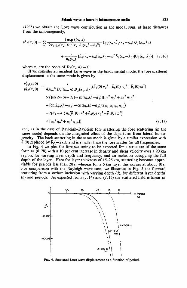
(1 935) we obtain the Love wave contribution as the modal sum, at large distances from the inhomogeneity,
where K, are the roots of D, ( K ~ , 12) = 0.
displacement in the same mode is given by If we consider an incident Love wave in the fundamental mode, the fore scattered
x([sh 2~o(h -d i ) - sh2~o(~-dz ) l [~oz VO’+PZ’ 1 2 0 ~ 1
+ [ch 2rto(/~-d,)-Ch 2tlo(h-d2)12P2 Po ?o v 2 0 )
- 2(dZ -dl) ‘lo( 6l (O) ?’ + 66 (0) KOz - 65 (0) O2)
x [PoZ ‘ lo2 + Pz2 tlzol) (7.17)
and, as in the case of Rayleigh-Rayleigh fore scattering the fore scattering (in the same mode) depends on the integrated effect of the departures from lateral homo- geneity. The back scattering in the same mode is given by a similar expression with 6i(0) replaced by 6,( - 2 ~ ~ ) ~ and is smaller than the fore scatter for all frequencies.
In Fig. 4 we plot the fore scattering to be expected for a structure of the same form as (6.28) with a 10 per cent increase in density and shear velocity over a 20 km region, for varying layer depth and frequency, and an inclusion occupying the full depth of the layer. Here for layer thickness of 15-25 km, scattering becomes appre- ciable for periods less than 20 s, whereas for a 5 km layer this occurs at about 10 s. For comparison with the Rayleigh wave case, we illustrate in Fig. 5 the forward scattering from a surface inclusion with varying depth (d), for different layer depths (h) and periods. As expected from (7.14) and (7.15) the scattered field is linear in
FIG. 4. Scattered Love wave displacement as a function of period.

324 B. L. N. Kennett
-0.02 \ \ \ 1
-0.04 -
. /----
0 0' \ 0 2 0-4 086 0 8
h 0 .-.
-0.02 -
-0.04 - - h = 15 0. Period 13.0s
-0.06 1 \ \. h . 2 5 0 . Period 12.95
FIG. 5. Dependence of scattered Love wave displacement on depth of inclusion/ depth of layer
dlh for d/h R 0 and dlh R 1. Again there are phase changes in the forward scattering, arising from interference effects but here depending on the waveguide character of the upper layer. The relative excitation of higher Love wave modes is dependent on the configuration of the inclusion with respect to the nodal points in their displace- ment patterns in the upper layer.
The disappearance of forward scattering from a lateral inhomogeneity at the point of phase change may help to explain the existence of spectral windows at short periods in some surface wave records.
Acknowledgment
The author would like to thank Dr E. R. Lapwood for advice and encouragement, and the Chairman and Directors of the British Petroleum Company Ltd for a Research Studentship and permission to publish this paper.
Department of Applied Mathematics and Theoretical Physics, Silver Street,
Cambridge, CB3 9EW
References
Bhattacharya, S . N., 1970. Love wave dispersion in a laterally heterogeneous layer lying over a homogeneous semi-infinite medium, Geophys. J. R. ustr. SOC., 19,
Babich, V. M. & Molotkov, I. A., 1966. The propagation of Love waves in an elastic half space which is inhomogeneous in the direction of two coordinates, Izv ANSSSR, Phys Solid Earth, 364-366.
Dunkin, J. W., 1965. Computation of modal solutions in layered, elastic media at high frequencies, Bull. seism SOC. Am., 55, 335-358.
361-366.

Seismic waves in laterally inhomogeneous media 325
Ewing, M., Jardetsky. W. &Press, F., 1957. Elastic Wavesin LayeredMedia, McGraw- Hill, New York.
Gilbert, F. & Backus, G. E., 1966. Propagator matrices in elastic wave and vibration problems, Geophysics., 31, 326-332.
Hadamard, J . , 1893. Resolution d’une question relative aux determinants, Bull. Sci. Math., 17, 240-246.
Haskell, N. A., 1953. The dispersion of surface waves on multilayered media, Bull. seism. SOC. Am., 43, 17-34.
Herrera, I. & Mal, A. K., 1965. A perturbation method for elastic wave propagation: 2. Small inhomogeneities, J. geophys, Res., 70, 871-883.
Herrin, E., 1969. Regional variations of P-wave velocity in the Upper Mantle beneath N. America in The Earth’s Crust and Upper Mantle: Geophysical Monograph 13, Am. geophys Un. Wash., 242-246.
Hudson, J. A. & Knopoff, L., 1966. Signal generated seismic noise, Geophys. J . R . astr. SOC., 11, 19-24.
Hudson, J. A. & Knopoff, L., 1967. Statistical properties of Rayleigh waves due to scattering by topography, Bull. seism. SOC. Am., 57, 83-90.
James, D. E. & Steinhart, J. S., 1966. Structure beneath continents: a critical review of explosion studies 1960-1965 in The Earth beneath the Continents: Geophysical Monograph 10, Am. geophys Un. Wash., 293-333.
Lapwood, E. R., 1949. The disturbance due to a line source in a semi-infinite elastic medium, Phil. Trans. R. SOC. A , 242, 63-100.
Mukhina, 1. V. & Molotkov, I. A., 1967. The Propagation of Rayleigh waves in an elastic half-space that is inhomogeneous in two coordinates, Izv. ANSSSR Phys. Solid Earth, 209-21 1.
Sezawa, K., 1935. Love waves generated from a source of a certain depth, Bull Earthq. Res. Inst., Tokyo, 13, 1-17.
Thomson, W. T., 1950. Transmission of elastic waves through a stratified solid medium, J. appl. Phys., 21, 89-93.
Zharkov, V. N. & Osnach, A. I., 1970. A perturbation theory for surface waves, Izv. ANSSSR Fiz. Zernli, No. 12, 1Ck21.