1SCIEntIfIC RepoRtS | (2018) 8:3098 | DOI:10.1038/s41598-018-20992-z

www.nature.com/scientificreports

Seismic waveform simulation for models with fluctuating interfacesYing Rao1,2 & Yanghua Wang 2

The contrast of elastic properties across a subsurface interface imposes a dominant influence on the seismic wavefield, which includes transmitted and reflected waves from the interface. Therefore, for an accurate waveform simulation, it is necessary to have an accurate representation of the subsurface interfaces within the numerical model. Accordingly, body-fitted gridding is used to partition subsurface models so that the grids coincide well with both the irregular surface and fluctuating interfaces of the Earth. However, non-rectangular meshes inevitably exist across fluctuating interfaces. This non-orthogonality degrades the accuracy of the waveform simulation when using a conventional finite-difference method. Here, we find that a summation-by-parts (SBP) finite-difference method can be used for models with non-rectangular meshes across fluctuating interfaces, and can achieve desirable simulation accuracy. The acute angle of non-rectangular meshes can be relaxed to as low as 47°. The cell size rate of change between neighbouring grids can be relaxed to as much as 30%. Because the non-orthogonality of grids has a much smaller impact on the waveform simulation accuracy, the model discretisation can be relatively flexible for fitting fluctuating boundaries within any complex problem. Consequently, seismic waveform inversion can explicitly include fluctuating interfaces within a subsurface velocity model.

Structural complexities such as the fluctuations of subsurface interfaces significantly influence seismic wavefields. For instance, fluctuating interfaces have both focusing and defocusing effects on seismic amplitudes. These interface-related amplitude effects can be exploited to reconstruct the interface geometry by inverting the seismic amplitudes1–5, and are also included implicitly in the waveform inversion of seismic reflection data6. Seismic reflection data, which are dominated by pre-critical reflected energy from subsurface contrasts in physical param-eters, are suitable for structural imaging following seismic migration. However, these data can also be utilised in waveform inversions to quantitatively reconstruct velocity models for the subsurface of the Earth6. These reflec-tion data are routinely recorded during explorations for hydrocarbons and mainly comprise of seismic P-wave data. Therefore, this paper uses an acoustic wave equation for a waveform simulation within an anisotropic medium.

To conduct an accurate waveform simulation for seismic waveform inversion, it is necessary to have an accu-rate representation of the subsurface interfaces within the numerical model, as the contrast in elastic properties across an interface has a dominant impact on the seismic wavefield. One of the suitable methods for wave-form simulation is the finite-element method, since either an irregular surface or fluctuating interfaces can be described well by triangular gridding, including an adaptive meshing scheme7,8. The finite-element method is computationally expensive in comparison to a finite-difference method. A finite-difference method can be used with triangular grids9, but the errors in spatial derivative computations on unstructured grids were counteracted by using grids of higher node density. It is also computationally expensive.

A straightforward and cost-effective waveform simulation method is the finite-difference method with quad-rilateral grids. In this paper, we adopt a body-fitted gridding scheme to partition each horizontal layer that is confined by two fluctuating interfaces in the model. Rao and Wang10 proposed strategies to produce grids for the irregular surface of Earth, to coincide with fluctuations of the surface while satisfying the pseudo-orthogonality condition. This pseudo-orthogonality condition is necessary to effectively avoid any scattering caused by artificial stair-type grids used within conventional rectangular gridding11,12. However, for a fluctuating interface, it is dif-ficult to simultaneously adjust such grids on both sides of the interface, and to ensure that grids across the inter-face satisfy the pseudo-orthogonality condition. Nevertheless, we reveal in this paper that a summation-by-parts

1State Key Laboratory of Petroleum Resources and Prospecting, China University of Petroleum (Beijing), Beijing, 102249, China. 2Centre for Reservoir Geophysics, Department of Earth Science and Engineering, Imperial College London, London, SW7 2BP, UK. Correspondence and requests for materials should be addressed to Y.W. (email: yanghua.wang@imperial.ac.uk)

Received: 14 August 2017

Accepted: 29 January 2018

Published: xx xx xxxx

OPEN

www.nature.com/scientificreports/

2SCIEntIfIC RepoRtS | (2018) 8:3098 | DOI:10.1038/s41598-018-20992-z

(SBP) discretisation approach may be effective for the finite-difference implementation of the wave equation. The SBP discretisation satisfies the SBP identity in Abel’s lemma13 that guarantees the stability of the finite-difference scheme14–18. We demonstrate that this SBP finite-difference method can cope with non-rectangular meshes in the vicinity of a fluctuating interface, and consequently achieve a desirable accuracy for the waveform simulation.

We focus on an acoustic waveform simulation and use a pseudo-acoustic wave equation for tilted transversely isotropic (TTI) media that are defined by two anisotropic parameters19. We extend this pseudo-acoustic wave equation to a model with surface and interface fluctuations. For a model that consists of an arbitrary number of interfaces, we apply the body-fitted gridding to each individual layer confined by two fluctuating interfaces. Non-rectangular meshes will become rectangular ones in the computational space through conformal mapping20. We reformulate the pseudo-acoustic wave equation and also derive the absorbing boundary condition, using the perfectly matched layer method21 in the computational space.

The quality of the meshing scheme in the physical space (before conformal mapping), determines the accuracy of the waveform simulation when utilising a finite-difference scheme. For instance, a low meshing quality reflects the characteristics of non-rectangular meshes, non-smoothness or abrupt mesh variations. The execution of the SBP finite-difference method leads to an improvement of the accuracy of the waveform simulation, by mitigating instability and coping with the low meshing qualities of body-fitted grids along the irregular surface of Earth, and along fluctuating interfaces.

Wave equation in consideration of fluctuating interfacesThe pseudo-acoustic wave equation for TTI media is defined by two anisotropic parameters, namely, ε and δ, which measure the difference between the two axes of the elliptical wavefront and the deviation from a perfect elliptical shape respectively22. The pseudo-acoustic wave equation is19

∂∂

=

+ −

− +

( ) ( )t

pq

v H v H v v H

v v H v H v Hpq

( )

( ),

(1)

px x sz z pz sz z

pn sz x sz x pz z

2

2

2 2 2 2

2 2 2 2

where p is the P wavefield, q is the auxiliary wavefield, vpz and vsz are the P-wave and SV-wave velocities respec-tively, along the axis of symmetry, vpx is the P-wave velocity perpendicular to the axis of symmetry, vpn is the P-wave normal-moveout velocity, and Hx and Hz are two 2D differential operators, ≡ ∂ ∂ ˆH x/x

2 2 and ≡ ∂ ∂ ˆH z/z2 2,

with respect to the rotated coordinate system (x, z). The last two anisotropic velocities (vpx, vpn) are related to the two anisotropy parameters ε and δ by22 ε= +v v 1 2px pz and δ= + .v v 1 2pn pz Note that for the P-wave simu-lation, the SV-wave velocity vsz remaining in eq. (1) does not have a significant effect on the wavefield.

In eq. (1), the two 2D differential operators in the Cartesian coordinate system (x, z) are16

φ φ φ

=∂∂

+∂∂

−

=∂∂

+∂∂

+∂

∂ ∂

Hx z

H

Hx z x z

,

sin cos sin2 ,(2)

x z

z

2

2

2

2

22

22

2

2

2

where φ is the dip angle of the axis of symmetry z, measured anticlockwise from the vertical direction z (Fig. 1a). In consideration of fluctuations in the Earth’s surface and of the subsurface interfaces, we use a body-fitted grid-ding method23. For any horizontal layer confined by two fluctuating interfaces, we transform the differential operators in eq. (2), from the Cartesian coordinate system (x, z) to the computational space (ξ, η) (Fig. 1b).

In the computational space, the second-order spatial derivatives are

ξξ

ξ ξξ η

η ηξ η

ξ ηη

η

ξξ

ξ ξξ η

η ηξ η

ξ ηη

η

ξξ ξ

ξ ξξ η

η ηξ η

ξ ηη η

η

∂∂

=∂∂

∂∂

+∂∂

∂∂

+∂∂

∂∂

+∂∂

∂∂

∂∂

=∂∂

∂∂

+∂∂

∂∂

+∂∂

∂∂

+∂∂

∂∂

∂∂ ∂

=∂∂

∂∂

+∂∂

∂∂

+∂∂

∂∂

+∂∂

∂∂

x

z

x z

,

,

,(3)

x x x x x x

z z z z z z

x z x z z x x z

2

22 2

2

22 2

2

where ξ ξ= ∂ ∂ x/ ,x ξ ξ= ∂ ∂� �z/ , ,z are assumed to be known parameters. Subsequently, substituting these spatial derivatives into the 2D differential operators Hx and Hz, we obtain the pseudo-acoustic wave eq. (1) in the com-putational space.

The SBP finite-difference methodTo avoid instabilities in numerical simulations caused both by low meshing precisions during body-fitted grid-ding and especially by strong variations in cell sizes, we propose an SBP finite-difference method that is uncondi-tionally stable24–26. In this SBP method, the spatial derivatives in eq. (3) are represented as

www.nature.com/scientificreports/

3SCIEntIfIC RepoRtS | (2018) 8:3098 | DOI:10.1038/s41598-018-20992-z

ξ ξ η ξ η η

ξ ξ η ξ η η

ξ ξ ξ η ξ η η η

∂∂

= + + +

∂∂

= + + +

∂∂ ∂

= + + +

ξ ξ ξ ξ η η ξ η η η

ξ ξ ξ ξ η η ξ η η η

ξ ξ ξ ξ η η ξ η η η

− + − +

− + − +

− + − +

xD E D D D D D D E D

zD E D D D D D D E D

x zD E D D D D D D E D

( ( ) ) ( ) ( ) ( ( ) ),

( ( ) ) ( ) ( ) ( ( ) ),

( ( ) ) ( ) ( ) ( ( ) ),(4)

x x x x x x

z z z z z z

x z x z z x x z

2

2 1/22

0 0 0 0 1/22

2

2 1/22

0 0 0 0 1/22

2

1/2 0 0 0 0 1/2

where = −+−

+D p h p p( ) ( )rj j

11 and = −−

−−D p h p p( ) ( )r

j j1

1 are the forward and backward differential operators, respectively, = −−

+ −D p h p p( ) ( )/2rj j0

11 1 is the central differential operator, = +ξ

+E p p p( ) ( )/2j j j1/2 1 is an average value for pj + 1/2, and h is the spatial sampling interval of either ξ or η.

The differential operators Hx and Hz in eq. (2) are then expressed explicitly as

ξ ξ η ξ η η

ξ ξ η ξ η η

φ ξ ξ η ξ η η

φ ξ ξ η ξ η η

φ ξ ξ ξ η ξ η η η

= + + +

+ + + +

−

= + + +

+ + + +

+ + + + .

ξ ξ ξ ξ η η ξ η η η

ξ ξ ξ ξ η η ξ η η η

ξ ξ ξ ξ η η ξ η η η

ξ ξ ξ ξ η η ξ η η η

ξ ξ ξ ξ η η ξ η η η

− + − +

− + − +

− + − +

− + − +

− + − +

H D E D D D D D D E D

D E D D D D D D E DH

H D E D D D D D D E D

D E D D D D D D E D

D E D D D D D D E D

( ( ) ) ( ) ( ) ( ( ) )

( ( ) ) ( ) ( ) ( ( ) ),

sin [ ( ( ) ) ( ) ( ) ( ( ) )]

cos [ ( ( ) ) ( ) ( ) ( ( ) )]

sin2 [ ( ( ) ) ( ) ( ) ( ( ) )] (5)

x x x x x x x

z z z z z z

z

z x x x x x x

z z z z z z

x z x z z x x z

1/22

0 0 0 0 1/22

1/22

0 0 0 0 1/22

21/2

20 0 0 0 1/2

2

21/2

20 0 0 0 1/2

2

1/2 0 0 0 0 1/2

We have thus completed the discretisation of the pseudo-acoustic wave equation using the SBP finite-difference method. Due to the presence of fluctuating interfaces within the model, we performed this dis-cretisation in the computational space (ξ, η).

ResultsAfter the model has been partitioned using body-fitted grids, the meshing quality will ultimately determine the numerical accuracy of the waveform simulation with a finite-difference method. Conventional finite-difference methods for isotropic media impose strict requirements on the qualities of body-fitted grids10. The requirements for such grids include two aspects: the acute angle of the grids should be >67°, and the rate of change in the cell size between neighbouring grids should be <5%.

Figure 1. The TTI media and the computational space. (a) Within homogeneous TTI media, the dip angle of the axis of symmetry of a wavefront is φ. The ray vector points from the source to the receiver. (b) In consideration of fluctuations of the Earth’s surface and of subsurface interfaces, body-fitted grids are transformed from the Cartesian space (x, y) to a computational space (ξ, η).

www.nature.com/scientificreports/

4SCIEntIfIC RepoRtS | (2018) 8:3098 | DOI:10.1038/s41598-018-20992-z

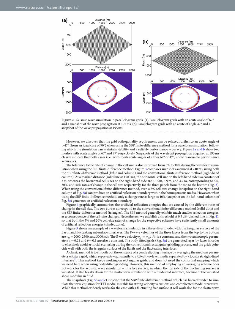
However, we discover that the grid orthogonality requirement can be relaxed further to an acute angle of >47° (from an ideal case of 90°) when using the SBP finite-difference method for a waveform simulation, follow-ing which the simulation can maintain stability and a reliable performance accuracy. Figure 2a and b show two meshes with acute angles of 67° and 47° respectively. Snapshots of the wavefront propagation acquired at 195 ms clearly indicate that both cases (i.e., with mesh acute angles of either 67° or 47°) show reasonable performance accuracies.

The tolerance to the rate of change in the cell size is also improved from 5% to 30% during the waveform simu-lation when using the SBP finite-difference method. Figure 3 compares snapshots acquired at 240 ms, using both the SBP finite-difference method (left-hand column) and the conventional finite-difference method (right-hand column). At a marked distance (solid line at 1500 m), the horizontal cell size on the left-hand side is a constant of 3 m, whereas the horizontal cell sizes on the right-hand side are 3.15 m, 3.9 m, and 4.2 m, corresponding to 5%, 30%, and 40% rates of change in the cell size respectively, for the three panels from the top to the bottom (Fig. 3). When using the conventional finite-difference method, even a 5% cell-size change (snapshot on the right-hand column of Fig. 3a) can produce an artificial reflection boundary within the homogeneous media. However, when using the SBP finite-difference method, only a change rate as large as 40% (snapshot on the left-hand column of Fig. 3c) generates an artificial reflection boundary.

Figure 4 graphically summarises the artificial reflection energies that are caused by the different rates of change in the cell size. The two curves correspond to the conventional finite-difference method (solid dots) and the SBP finite-difference method (triangles). The SBP method generally exhibits much smaller reflection energies, as a consequence of the cell-size changes. Nevertheless, we establish a threshold at 0.5 dB (dashed line in Fig. 4), so that both the 5% and 30% cell-size rates of change for the respective schemes have sufficiently small amounts of artificial reflection energies (shaded zone).

Figure 5 shows an example of a waveform simulation in a three-layer model with the irregular surface of the Earth and fluctuating subsurface interfaces. The P-wave velocities of the three layers from the top to the bottom are vpz = 2000, 2500, and 3000 m/s. The S-wave velocity =v v / 3sz pz is a constant, and the two anisotropic param-eters ε = 0.24 and δ = 0.1 are also a constant. The body-fitted grids (Fig. 5a) are generated layer-by-layer in order to effectively avoid artificial scattering during the conventional rectangular gridding process, and the grids coin-cide well with both the irregular surface of the Earth and the fluctuating interfaces.

A classic method is to smooth out the existence of a gently dipping interface by averaging the medium param-eters within a grid, which represents equivalently to a tilted two-layer media separated by a locally straight-lined interface27. This method keeps working on rectangular grids, and does not need the conformal mapping which we need here when using body-fitted gridding. However, this method of employing an averaging scheme does not work for the acoustic wave simulation with a free surface, in which the top side of the fluctuating surface is vanished. It also breaks down for the elastic wave simulation with a fluid/solid interface, because of the vanished shear modulus in fluid.

The snapshots (Fig. 5b and c) indicate that the SBP finite-difference method, which has been extended to sim-ulate the wave equation for TTI media, is stable for strong velocity variations and complicated model structures. While this method evidently works for the case with a fluctuating free surface, it will work also for the elastic wave

Figure 2. Seismic wave simulation in parallelogram grids. (a) Parallelogram grids with an acute angle of 67° and a snapshot of the wave propagation at 195 ms. (b) Parallelogram grids with an acute of angle 47° and a snapshot of the wave propagation at 195 ms.

www.nature.com/scientificreports/

5SCIEntIfIC RepoRtS | (2018) 8:3098 | DOI:10.1038/s41598-018-20992-z

simulation with a fluid/solid interface, as it avoids averaging an elastic medium with a vanished shear modulus in fluid.

ConclusionsBody-fitted gridding schemes are effective for partitioning numerical models within seismic waveform sim-ulations when considering complex fluctuations of both the Earth’s surface and the subsurface interfaces. However, when these schemes are used to fit these complex fluctuations, non-rectangular meshes are inevitably generated across the interfaces, and the resulting grids cannot always satisfy the pseudo-orthogonality condi-tion. The non-orthogonality of the meshing will degrade the precision of the mesh, and reduce the accuracy of the waveform simulation. This paper revealed that when using the proposed SBP finite-difference method, non-rectangular meshes can be included within the implementation of a waveform simulation. The acute angle of the grids may be relaxed to as low as 47° (from an ideal case of 90°), and the rate of change in the cell size could

Figure 3. Wavefield simulation in grids with different change rates of the cell size. (a) The rate of change in the cell size is 5% at the marked (solid line) distance of 1500 m. (b) The rate of change is 30% at the marked distance. (c) The rate of change is 40% at the marked distance. The left-hand column illustrates snapshots (at 240 ms) of the SBP finite-difference method, and the right-hand column illustrates snapshots of the conventional finite-difference method.

www.nature.com/scientificreports/

6SCIEntIfIC RepoRtS | (2018) 8:3098 | DOI:10.1038/s41598-018-20992-z

Figure 4. The artificial reflection energy (in dB). The artificial reflections are caused by different rates of change in the cell size. The solid dots show the artificial reflection energies from the conventional finite-difference method, and the triangles represent the artificial reflection energies from the SBP finite-difference method. The shaded zone represents the sufficiently small artificial reflection energies that are less than 0.5 dB (dashed line) for different rates of change in the cell size.

Figure 5. Wave simulation in a model with a fluctuating surface and interfaces. (a) A three-layer velocity model that is masked by body-fitted gridding. The body-fitted grids coincide well with both the irregular surface and the fluctuating interfaces of Earth. (b) Snapshot of the wavefield at 85 ms. (c) Snapshot of the wavefield at 207 ms.

www.nature.com/scientificreports/

7SCIEntIfIC RepoRtS | (2018) 8:3098 | DOI:10.1038/s41598-018-20992-z

be relaxed to as much as 30%. By contrast, these two quantities are 67° and 5% respectively, when using the con-ventional finite-difference method5. Therefore, when using the SBP finite-difference method, the body-fitted grids can be more flexible to fit fluctuating boundaries that confine any subsurface layer, and the non-orthogonality of the meshing scheme has a smaller impact on the accuracy of the waveform simulation. Therefore, seismic wave-form inversion for velocity imaging endeavours is capable of explicitly including fluctuating interfaces within a subsurface model.

References 1. Wang, Y. & Houseman, G. A. Inversion of reflection seismic amplitude data for interface geometry. Geophysical Journal International

117, 92–110, https://doi.org/10.1111/j.1365-246X.1994.tb03305.x (1994). 2. Wang, Y. & Houseman, G. A. Tomographic inversion of reflection seismic amplitude data for velocity variation. Geophysical Journal

International 123, 355–372, https://doi.org/10.1111/j.1365-246X.1995.tb06859.x (1995). 3. Wang, Y. & Pratt, R. G. Seismic amplitude inversion for interface geometry of multi-layered structures. Pure and Applied Geophysics

157, 1601–1620, https://doi.org/10.1007/PL00001052 (2000). 4. Wang, Y., White, R. E. & Pratt, R. G. Seismic amplitude inversion for interface geometry: practical approach for application.

Geophysical Journal International 142, 162–172, https://doi.org/10.1046/j.1365-246x.2000.00144.x (2000). 5. Wang, Y. Seismic Amplitude Inversion in Reflection Tomography (Elsevier 2003). 6. Wang, Y. & Rao, Y. Reflection seismic waveform tomography. Journal of Geophysical Research 114, B03304, https://doi.

org/10.1029/2008JB005916 (2009). 7. Michelini, A. An adaptive-grid formalism for traveltime tomography. Geophysical Journal International 121, 489–510, https://doi.

org/10.1111/j.1365-246X.1995.tb05728.x (1995). 8. Sambridge, M. & Faletic, R. Adaptive whole Earth tomography. Geochemistry, Geophysics, Geosystems 4(3), 1022, https://doi.

org/10.1029/2001GC000213 (2003). 9. Käser, M. & Igel, H. Numerical simulation of 2D wave propagation on unstructured grids using explicit differential operators.

Geophysical Prospecting 49, 607–619, https://doi.org/10.1046/j.1365-2478.2001.00276.x (2001). 10. Rao, Y. & Wang, Y. Seismic waveform simulation with pseudo-orthogonal grids for irregular topographic models. Geophysical

Journal International 194, 1778–1788, https://doi.org/10.1093/gji/ggt190 (2013). 11. Zhang, W. & Chen, X. F. Traction image method for irregular free surface boundaries in finite difference seismic wave simulation.

Geophysical Journal International 167, 337–353, https://doi.org/10.1111/j.1365-246X.2006.03113.x (2006). 12. Zhang, Z. G., Zhang, W. & Chen, X. F. Complex frequency-shifted multi-axial perfectly matched layer for elastic wave modelling on

curvilinear grids. Geophysical Journal International 198, 140–153, https://doi.org/10.1093/gji/ggu124 (2014). 13. Guenther R. B. & Lee L. W. Partial Differential Equations of Mathematical Physics and Integral Equations (Dover Publications

1996). 14. Strand, B. Summation by parts for finite difference approximations for d/dx. Journal of Computational Physics 110, 47–67, https://

doi.org/10.1006/jcph.1994.1005 (1994). 15. Mattsson, K. & Nordström, J. Summation by parts operators for finite difference approximations of second derivatives. Journal of

Computational Physics 199, 503–540, https://doi.org/10.1016/j.jcp.2004.03.001 (2004). 16. Svärd, M., Mattsson, K. & Nordström, J. Steady-state computations using summation-by-parts operators. Journal of Scientific

Computing 24, 79–95, https://doi.org/10.1007/s10915-004-4788-2 (2005). 17. Mattsson, K. Summation by parts operators for finite difference approximations of second-derivatives with variable coefficients.

Journal of Scientific Computing 51, 650–682, https://doi.org/10.1007/s10915-011-9568-1 (2012). 18. Petersson, N. A. & Sjogreen, B. Super-grid modelling of the elastic wave equation in semi-bounded domains. Communications in

Computational Physics 16, 913–955, https://doi.org/10.4208/ cicp.290113.220514a (2014). 19. Fletcher, R. P., Du, X. & Fowler, P. J. Reverse time migration in tilted transversely isotropic (TTI) media. Geophysics 74(6),

WCA179–WCA187, https://doi.org/10.1190/1.3269902 (2009). 20. Fornberg, B. The pseudospectral method: accurate representation of interfaces in elastic wave calculations. Geophysics 53, 625–637,

https://doi.org/10.1190/1.1442497 (1988). 21. Berenger, J. P. 1994 A perfectly matched layer for the absorption of electromagnetic waves. Journal of Computational Physics 114,

185–200, https://doi.org/10.1006/jcph.1994.1159 (1994). 22. Thomsen, L. Weak elastic anisotropy. Geophysics 51, 1954–1966, https://doi.org/10.1190/1.1442051 (1986). 23. Komatitsch, D., Coute, F. & Mora, P. Tensorial formulation of the wave equation for modelling curved interfaces. Geophysical Journal

International 127, 156–168, https://doi.org/10.1111/j.1365-246X.1996.tb01541.x (1996). 24. Kreiss, H. O. & Scherer, G. Finite element and finite difference methods for hyperbolic partial differential equations. Mathematical

Aspects of Finite Elements in Partial Differential Equations (ed. de Boor, C.), 195–212 (Academic Press 1974). 25. Nilsson, S., Petersson, N. A. & Sjögreen, B. Stable difference approximations for the elastic wave equation in second order

formulation. SIAM Journal on Numerical Analysis 45, 1902–1936, https://doi.org/10.1137/060663520 (2007). 26. Sjögreen, B. & Petersson, N. A. A fourth order accurate finite difference scheme for the elastic wave equation in second order

formulation. Journal of Scientific Computing 52, 17–48, https://doi.org/10.1007/s10915-011-9531-1 (2012). 27. Muir, F., Dellinger, J., Etgen, J. & Nichols, D. Modeling elastic fields across irregular boundaries. Geophysics 57, 1189–1193, https://

doi.org/10.1190/1.1443332 (1992).

AcknowledgementsThe authors are grateful to the National Natural Science Foundation of China (grant nos. 41474111, and 41622405), the Science Foundation of China University of Petroleum (Beijing) (grant no. 2462018BJC001), and the sponsors of the Centre for Reservoir Geophysics, Imperial College London, for supporting this research.

Author ContributionsY.R. implemented the algorithm and conducted the numerical simulation. Y.W. focused on the innovative concepts and finalised the paper. All authors contributed to the preparation of the figures and the revision of the paper.

Additional InformationCompeting Interests: The authors declare no competing interests.Publisher's note: Springer Nature remains neutral with regard to jurisdictional claims in published maps and institutional affiliations.

www.nature.com/scientificreports/

8SCIEntIfIC RepoRtS | (2018) 8:3098 | DOI:10.1038/s41598-018-20992-z

Open Access This article is licensed under a Creative Commons Attribution 4.0 International License, which permits use, sharing, adaptation, distribution and reproduction in any medium or

format, as long as you give appropriate credit to the original author(s) and the source, provide a link to the Cre-ative Commons license, and indicate if changes were made. The images or other third party material in this article are included in the article’s Creative Commons license, unless indicated otherwise in a credit line to the material. If material is not included in the article’s Creative Commons license and your intended use is not per-mitted by statutory regulation or exceeds the permitted use, you will need to obtain permission directly from the copyright holder. To view a copy of this license, visit http://creativecommons.org/licenses/by/4.0/. © The Author(s) 2018