Seismic Velocity Estimation from Time Migration Velocities

M. K. Cameron, S. B. Fomel, J. A. Sethian ∗

October 10, 2006

Submitted for Publication: Inverse Problems, Oct. 2006

Abstract

We address the problem of estimating seismic velocities inside the earth which is necessaryfor obtaining seismic images in regular Cartesian coordinates. We derive a relation between thetrue seismic velocities and the routinely obtained so called ”time migration velocities”, whichare some kind of mean velocities. We formulate an inverse problem and show that it is ill-posed.We suggest three different approaches for solving it. We test these algorithms on synthetic dataand apply them to a field data example.

1 Introduction

Seismic data are the records of the pressure wave amplitudes P described by the wave equation

∆P (x, y, z; t) =1

v2(x, y, z)

∂2

∂t2P (x, y, z; t), (1)

where v(x, y, z), common referred to as the ”seismic velocity”, is the sound speed of the earth.This velocity is typically unknown, and its determination is the subject of the present work.

One common fast and robust process of obtaining seismic images is called time migration (seee.g. [Yilmaz, 2001]). This process is considered adequate for the areas with mild lateral velocityvariation, i.e. where v depends mostly on z and only slightly on x and y. However, even mildlateral velocity variations can significantly distort subsurface structures on the time migratedimages. Moreover, time migration produces images in very specific time migration coordinates(x0, t0) (explained below), and the relation between them and the Cartesian coordinates can benontrivial if the velocity varies laterally.

One “side product” of time migration is mean velocities vm(x0, t0), known as time migrationvelocities. We will refer to them as migration velocities for brevity. In the case where the seismicvelocity depends only on the depth, these velocities are close to the root-mean-square (RMS)velocities [Dix, 1955]. In the general case, these velocities relate to the radius of curvature ofthe emerging wave front [Hubral and Krey, 1980].

An alternative approach to obtaining seismic images is called depth migration [Yilmaz, 2001].This approach is adequate for areas with lateral velocity variation, and produces seismic images

∗This work was supported in part by the Applied Mathematical Science subprogram of the Office of Energy

Research, U.S. Department of Energy, under Contract Number DE-AC03-76SF00098, and by the Computational

Mathematics Program of the National Science Foundation

1

in regular Cartesian coordinates. The major problem with this approach is that its implemen-tation requires the construction of a velocity model for the seismic velocity v(x, y, z). It canbe both difficult and time consuming to construct an adequate velocity model: an iterativeapproach of guesswork followed by correction is often employed.

The main idea of this work is to construct a velocity model v(x) from the migration velocitiesgiven in the time migration coordinates (x0, t0) (see a block-scheme in Fig. 1) . Using thesevelocities one can then perform depth migration to obtain an improved seismic image in theCartesian coordinates x. As an alternative to depth migration, one can instead directly converta time migrated image to ”depth” (regular Cartesian coordinates) using the additional outputsof our construction x0(x) and t0(x).

Figure 1: The main idea of this work.

Thus, our goals are to create fast and robust algorithms to:

1. Convert the migration velocities vm(x0, t0) to the true seismic velocities v(x);

2. Convert time migrated images (in (x0, t0) coordinates) to ”depth” (to images in regularCartesian coordinates x).

The end result is to construct more accurate seismic images cheaply and routinely.Our results are the following. To this end, we have obtained theoretical relations between

the migration velocity and the true seismic velocity in 2D and 3D. It came out in the theoreticalrelation in 2D that the Dix velocities vDix(x0, t0) which are a conventional estimate of trueseismic velocities from the migration velocities, can be used instead of the migration velocitiesas a more convenient input. We have stated an inverse problem of finding the true seismicvelocity from the Dix velocity and developed two approaches for solving it: the ray tracingapproach and the level set approach.

These two approaches involve three numerical algorithms:

1. An efficient time-to-depth conversion algorithm;

2. A ray tracing algorithm;

3. A level set algorithm.

The relations between the approaches and the algorithms are outlined in the block-scheme inFig. 2.

2

Figure 2: The approaches and the algorithms.

1.1 Time migration coordinates and image rays

For many decades, seismic imaging was based on the assumption that the velocity inside theearth depends only on the depth and that the subsurface structures are horizontal or, at worst,planar with the same dipping angle. To obtain more complex structure distortions, Hubral[Hubral, 1977] introduced the concept of the image ray, which gives the connection between thetime migration coordinates and the regular Cartesian coordinates.

Figure 3: Image rays and time migration coordinates.

To explain this idea, we begin with the high frequency approximation applied to the waveequation (1), in which the wave front T (x, y, z) propagates according to the Eikonal equation(see e.g. [Popov, 2002]):

|∇T (x, y, z)|2 =1

v2(x, y, z). (2)

3

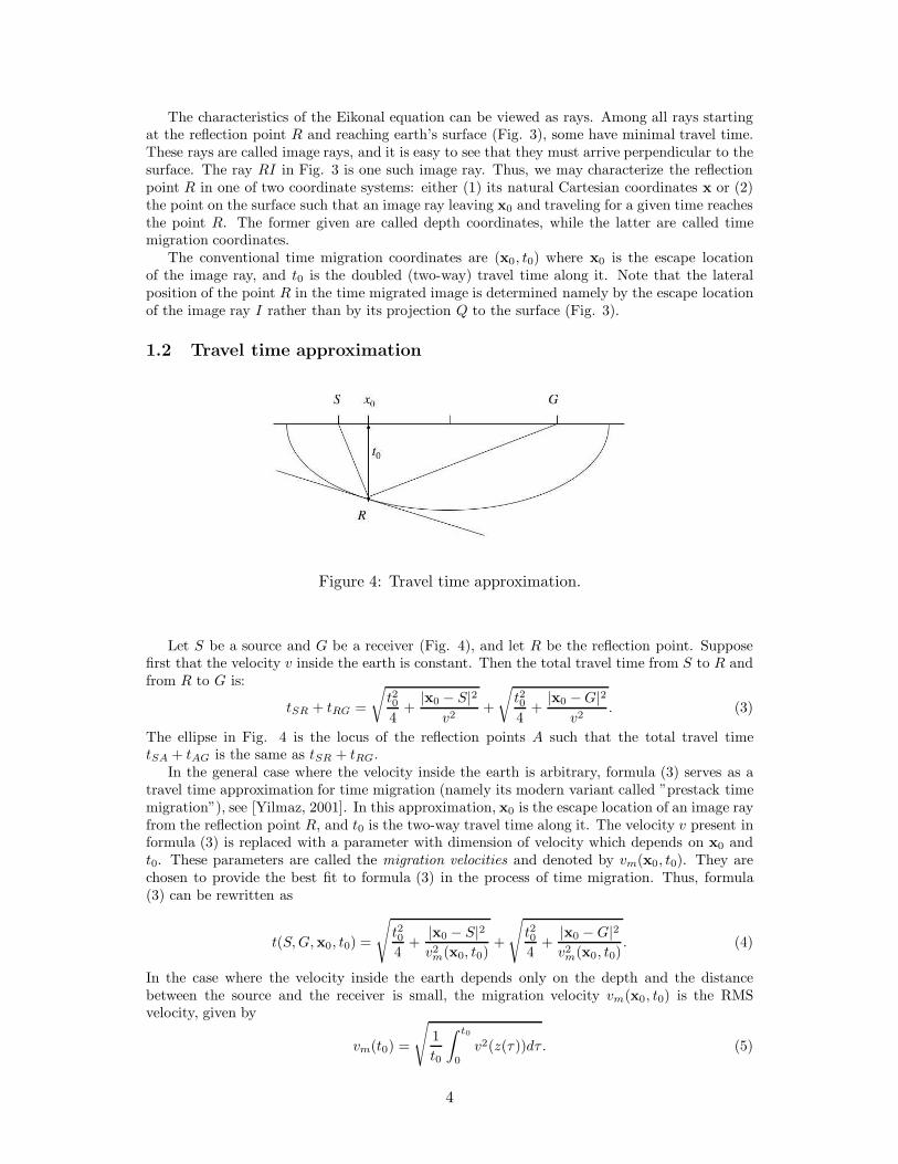
The characteristics of the Eikonal equation can be viewed as rays. Among all rays startingat the reflection point R and reaching earth’s surface (Fig. 3), some have minimal travel time.These rays are called image rays, and it is easy to see that they must arrive perpendicular to thesurface. The ray RI in Fig. 3 is one such image ray. Thus, we may characterize the reflectionpoint R in one of two coordinate systems: either (1) its natural Cartesian coordinates x or (2)the point on the surface such that an image ray leaving x0 and traveling for a given time reachesthe point R. The former given are called depth coordinates, while the latter are called timemigration coordinates.

The conventional time migration coordinates are (x0, t0) where x0 is the escape locationof the image ray, and t0 is the doubled (two-way) travel time along it. Note that the lateralposition of the point R in the time migrated image is determined namely by the escape locationof the image ray I rather than by its projection Q to the surface (Fig. 3).

1.2 Travel time approximation

Figure 4: Travel time approximation.

Let S be a source and G be a receiver (Fig. 4), and let R be the reflection point. Supposefirst that the velocity v inside the earth is constant. Then the total travel time from S to R andfrom R to G is:

tSR + tRG =

√

t204

+|x0 − S|2

v2+

√

t204

+|x0 − G|2

v2. (3)

The ellipse in Fig. 4 is the locus of the reflection points A such that the total travel timetSA + tAG is the same as tSR + tRG.

In the general case where the velocity inside the earth is arbitrary, formula (3) serves as atravel time approximation for time migration (namely its modern variant called ”prestack timemigration”), see [Yilmaz, 2001]. In this approximation, x0 is the escape location of an image rayfrom the reflection point R, and t0 is the two-way travel time along it. The velocity v present informula (3) is replaced with a parameter with dimension of velocity which depends on x0 andt0. These parameters are called the migration velocities and denoted by vm(x0, t0). They arechosen to provide the best fit to formula (3) in the process of time migration. Thus, formula(3) can be rewritten as

t(S, G, x0, t0) =

√

t204

+|x0 − S|2v2

m(x0, t0)+

√

t204

+|x0 − G|2v2

m(x0, t0). (4)

In the case where the velocity inside the earth depends only on the depth and the distancebetween the source and the receiver is small, the migration velocity vm(x0, t0) is the RMSvelocity, given by

vm(t0) =

√

1

t0

∫ t0

0

v2(z(τ ))dτ . (5)

4

.

1.3 Emerging wave front

In this section, our aim is to justify the travel time approximation given by formula (4).

Figure 5: Emerging wave front.

Consider an emerging wave front from a point source A (Fig. 5) [Hubral and Krey, 1980].Let the image ray arrive at the surface point (x0, y0) at time t0 (here t0 is the one-way traveltime along the image ray). The travel time from A to the surface along some other ray close tothe image ray, arriving at the surface point (x, y), is given by the Taylor expansion

t(x, y) = t0 +1

2∆xTΓ∆x + O(δ3), (6)

where ∆x =

(

x − x0

y − y0

)

, Γ is the matrix of the second derivatives of t(x, y) evaluated at

the point (x0, y0) and δ =√

(x − x0)2 + (y − y0)2. From geometrical considerations, one canobtain [Hubral and Krey, 1980] a relation between the matrix Γ and the matrix R of the radiiof curvature of the emerging wave front, namely

Γ−1 = Rv(x0, y0), (7)

where v(x0, y0) = v(x = x0, y = y0, z = 0) is the velocity at the surface point (x0, y0).In the case where sources and receivers are arranged along some straight line, seismic imaging

becomes a 2D problem, and equation (6) can be simplified to

t(x) = t0 +1

2(x − x0)

2txx(x = x0) + O(δ3) = t0 +(x − x0)

2

2Rv(x0)+ O(δ3), (8)

where v(x0) ≡ v(x = x0, z = 0). By squaring both sides of equation (8) we get:

t2(x) = t20 + (x − x0)2t0txx(x = x0) + O(δ3) = t20 + (x − x0)

2 t0Rv(x0)

+ O(δ3). (9)

Suppose we want to compute the total travel time from a source S to the reflection point A andfrom A to a receiver G. Using equation (9) we obtain:

t(x0, t0, S, G) = tSA + tAG =

√

t20 + (S − x0)2t0

Rv(x0)+

√

t20 + (G − x0)2t0

Rv(x0)+O(δ3). (10)

5

Comparing equations (10) and (4) we see that the travel time approximation given by formula(4) follows from the Taylor expansion in 2D. Moreover, the migration velocity and the radius ofcurvature of the emerging wave front are converted through the relation

t0v2m(x0, t0) = v(x0)R(x0, t0). (11)

On the other hand, in 3D the travel time approximation given by formula (4) is not aconsequence of the Taylor expansion as it is in 2D. Instead, one can easily derive the followingtravel time formula from equations (6) and (7):

t(x0, t0, S, G) =√

t20 + t0(S − x0)T [v(x0)R(x0, t0)]−1(S − x0) (12)

+√

t20 + t0(G − x0)T [v(x0)R(x0, t0)]−1(G − x0).

However note that if the velocity depends only on the depth, the matrix R is a multiple ofthe identity matrix, and hence formula (4) is the consequence of the Taylor expansion.

1.4 Dix inversion

Dix [Dix, 1955] established the first connection between the migration velocities and the seismicvelocities for the case where the velocity depends only on the depth. He showed that themigration velocities are the RMS velocities if the distances between the sources and the receiversare small and came up with the following inversion method. Consider an earth model as in Fig.

Figure 6: Dix inversion.

6. Let the layers be flat and horizontal, and the velocity be constant within each layer. We aregiven the RMS velocities Vi and the travel times ti, i = 1, 2, ..., n, where Vi is the RMS velocityof the first i layers with respect to the time, and ti is the two-way vertical travel time from theearth surface to the bottom of the i-th layer. Then the layer velocities (or as they are called ingeophysics ”interval velocities”) vi can be found successively from i = 2 to n:

vi =

√

V 2i ti − V 2

i−1ti−1

ti − ti−1. (13)

The depths of the lower boundaries of the layers are:

zi = zi−1 + viti − ti−1

2. (14)

6

Sometimes Dix inversion is applied to find the interval velocities from the migration velocitiesin the case where the velocity varies laterally. Then for the continuously changing velocity in2D the Dix velocities are given by:

v(x0, t0) =

√

∂

∂t0(t0v2

m(x0, t0)). (15)

2 Forward modeling of the time migration velocities

In this section we derive our main theoretical result: the relation between the migration velocitiesand the true seismic velocities in 2D and between the matrix Γ in formula (6) in 3D.

2.1 Paraxial ray tracing

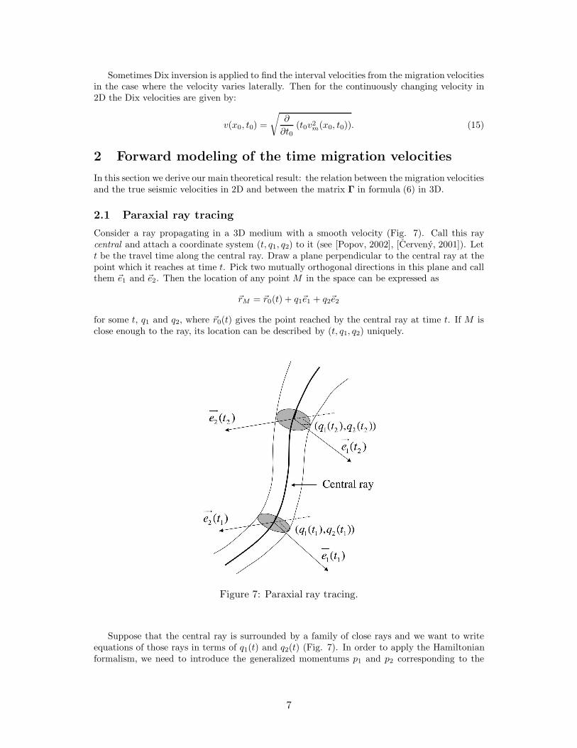
Consider a ray propagating in a 3D medium with a smooth velocity (Fig. 7). Call this raycentral and attach a coordinate system (t, q1, q2) to it (see [Popov, 2002], [Cerveny, 2001]). Lett be the travel time along the central ray. Draw a plane perpendicular to the central ray at thepoint which it reaches at time t. Pick two mutually orthogonal directions in this plane and callthem ~e1 and ~e2. Then the location of any point M in the space can be expressed as

~rM = ~r0(t) + q1~e1 + q2~e2

for some t, q1 and q2, where ~r0(t) gives the point reached by the central ray at time t. If M isclose enough to the ray, its location can be described by (t, q1, q2) uniquely.

Figure 7: Paraxial ray tracing.

Suppose that the central ray is surrounded by a family of close rays and we want to writeequations of those rays in terms of q1(t) and q2(t) (Fig. 7). In order to apply the Hamiltonianformalism, we need to introduce the generalized momentums p1 and p2 corresponding to the

7

generalized coordinates q1 and q2. We first note the fact that the central ray is a ray itself, andthis imposes the following requirements on the evolution of ~e1 and ~e2:

d~e1

dt=

∂v(t, q1, q2)

∂q1 q1=q2=0

~τ,d~e2

dt=

∂v(t, q1, q2)

∂q2 q1=q2=0

~τ ,

where ~τ is the unit tangent vector to the central ray ([Popov, 2002]). The ray equations in theHamiltonian form are ([Popov, 2002], [Popov and Psencik, 1978],[Cerveny, 2001]):

d

dt

(

qp

)

=

(

0 v20I2

− 1v0

V 0

)(

qp

)

. (16)

Here v0 is the velocity along the central ray, I2 is the 2 × 2 identity matrix, and V is a 2 × 2matrix of the second derivatives of the velocity:

Vij =∂2v(t, q1, q2)

∂qi∂qj, i, j = 1, 2.

Suppose that the family of rays depends upon two parameters (α1, α2). There are twoimportant cases:

• All rays start perpendicular to the same plane. Then (α1, α2) can be chosen to be theinitial coordinates (x0, y0) of the rays at this plane. We will call such a family of raystelescopic.

• All rays start at the same point, but in different directions. Then (α1, α2) can be chosento be the initial momentums (p1(0), p2(0)) of the rays. We will call such a family the pointsource family.

Consider the following 2 × 2 matrices ([Popov, 2002], [Cerveny, 2001]):

Qij ≡∂qi

∂αj, Pij ≡

∂pi

∂αj, i, j = 1, 2. (17)

The equations of time evolution for Q and P are the equations in variations for equation (16):

d

dt

(

Q

P

)

=

(

0 v20I2

− 1v0

V 0

)(

Q

P

)

. (18)

The initial conditions for the telescopic family of rays are

Q(0) = I2, P(0) = 0, (19)

and for the point source family they are

Q(0) = 0, P(0) =1

v0(0)I2, (20)

where v0(0) is the velocity at the source point. The absolute value of the determinant of thematrix Q has a nice geometrical sense ([Popov, 2002]):

| detQ| is the geometrical spreading of the family of rays.

Let the central ray arrive orthogonal to some plane at a point (x0, y0). Consider the matrixΓ of the second derivatives of the travel times of the family of rays around the central ray,evaluated at the point (x0, y0). E.g., the central ray can be the image ray arriving to the earthsurface. Then the matrix Γ is defined by formula 6) for the source point family of rays from thesource point A as in Fig. 5. In [Popov, 2002], [Cerveny, 2001] it was shown that

Γ = PQ−1 (21)

8

andd

dtΓ = −v2

0Γ2 − 1

v0V. (22)

For convenience, in the present work we will deal with the matrix K = Γ−1, which is the matrixof radii of curvature of the wave front scaled by the velocity at the image ray, namely

K = v0R = QP−1. (23)

One can easily derive from equation (22) that the time evolution of K is given by:

d

dtK = v2

0I2 +1

v0KVK. (24)

For the point source family of rays the initial conditions for the matrix K are:

K(0) = 0. (25)

2.2 Relation between the matrix K and the true seismic velocities in

3D

Theorem 1 Let an image ray starting from a subsurface point x (Fig. 8) arrive at the earthsurface point x0 at time t0. Designate this ray to be central. Let the matrix K(x0, t0) be evaluatedat the surface for a point source family of rays around the image ray, starting at the same pointx. Suppose there is also a telescopic family of rays around the image ray starting perpendicularto the earth surface which we trace backwards w.r.t. the image ray for time t0 and compute thematrices Q and P. Let Q(x0, t0) be the matrix Q for the telescopic family of rays evaluated atthe time t0 (i.e., at the subsurface point x) in this backward tracing. Then

∂

∂t0K(x0 , t0) = v2(x(x0, t0))

(

Q(x0, t0)TQ(x0, t0)

)−1. (26)

Figure 8: Illustration for Theorem 1.

9

Rewrite the travel time approximation (12) using the notation K:

t(x0, t0, S, G) =√

t20 + t0(S − x0)T [K(x0, t0)]−1(S − x0) (27)

+√

t20 + t0(G − x0)T [K(x0, t0)]−1(G − x0).

The matrix K in formula (27) is a matrix of parameters depending on x0 and t0, which can beestimated from the measurements. Theorem 1 provides a connection between the matrix K andthe true seismic velocity at the subsurface point x reached by the image ray arriving at x0 andtraced backwards for time t0 (Fig. 8).

Proof Let an image ray arrive at the surface point x0 at time t1. Fix a moment of time t0 < t1and consider a point source family of rays starting at the subsurface point x(x0, t0) which theimage ray passes at time t0. Introduce the following notations:

X =

(

Q

P

)

=

Q11 Q12

Q21 Q22

P11 P12

P21 P22

, A(t) =

(

0 v20I2

− 1v0

V 0

)

.

Let X∗ be the 4 × 4 matrix of derivatives of X with respect to the initial conditions:

X(t0) =

Q110 Q120

Q210 Q220

P110 P120

P210 P220

:

X∗ =

∂Q11

∂Q110

∂Q11

∂Q210

∂Q12

∂Q120

∂Q12

∂Q220

∂Q21

∂Q110

∂Q21

∂Q210

∂Q22

∂Q120

∂Q22

∂Q220

∂P11

∂P110

∂P11

∂P210

∂P12

∂P120

∂P12

∂P220

∂P21

∂P110

∂P21

∂P210

∂P22

∂P120

∂P22

∂P220

.

Note that since each of the columns of X is a linear independent solution of equation (16) thederivatives not included into X∗ are zeros. X(t) and X∗(t) are solutions of the following initialvalue problems:

dX

dt= A(t)X, X(t0) =

1

v(t0)

(

0

I2

)

, (28)

where v(t0) = v(x(x0, t0)), and

dX∗dt

= A(t)X∗, X∗(t0) = I4. (29)

Denote the solution of equation (29) by B(t0; t1) as it is done in [Cerveny, 2001]:

B(t0; t1) =

(

Q1 Q2

P1 P2

)

,

where Qi, Pi, i = 1, 2 are 2× 2 matrices.

(

Q1

P1

)

satisfies the initial conditions corresponding

to a telescopic point, and

(

Q2

P2

)

satisfies the initial conditions corresponding to a normalized

point source. B(t0, t1) is called the propagator matrix. Then the solution of (28) is:

X(t) =1

v(t0)

(

Q2

P2

)

. (30)

10

Now turn to the matrix K: K(t0; t1) = Q(t0; t1)P(t0; t1)−1 = Q2P

−12 .

Shift the initial time t0 by −∆t. Then, according to equation (28) at time t0

Q(t0 − ∆t; t0) = 0 + ∆tv2(t0)1

v(t0)I2 + O((∆t)2),

P(t0 − ∆t; t0) =1

v(t0)I2 + O((∆t)2).

Hence the change in the initial conditions for equation (28) is:

∆Q0 = v0∆tI2 + O((∆t)2), ∆P0 = 0 + O((∆t)2). (31)

Then

K(t0 − ∆t; t1) = K(t0; t1) +

2∑

i,j=1

∂K

∂Qij0∆Qij0 +

2∑

i,j=1

∂K

∂Pij0∆Pij0 + O((∆t)2) (32)

= K(t0; t1) +

(

∂K

∂Q110+

∂K

∂Q220

)

v(t0)∆t + O((∆t)2).

Let us find the partial derivatives in the expression above:

∂K

∂Qii0=

∂Q

∂Qii0P−1 − QP−1 ∂P

∂Qii0P−1, i = 1, 2. (33)

In terms of the entries of the matrix B(t0; t1)

∂K

∂Q110+

∂K

∂Q220= v0(Q1P

−12 − Q2P

−12 P1P

−12 ). (34)

In [Cerveny, 2001] the symplectic property of the matrix B(t0; t1) was proved:

BTJB = J, (35)

where J is the 4 × 4 matrix

J =

(

0 I2

−I2 0

)

.

To simplify formula (34) we will use the following consequences of the symplectic property (35):

PT2 Q1 − QT

2 P1 = I2, PT2 Q2 = QT

2 P2. (36)

Then the matrix expression in equation (34) simplifies to:

Q1P−12 − Q2P

−12 P1P

−12 =

(PT2 )−1PT

2 Q1P−12 − (PT

2 )−1PT2 Q2P

−12 P1P

−12 =

(PT2 )−1(PT

2 Q1 −PT2 Q2P

−12 P1)P

−12 =

(PT2 )−1(PT

2 Q1 −QT2 P2P

−12 P1)P

−12 =

(PT2 )−1(PT

2 Q1 −QT2 P1)P

−12 =

(PT2 )−1P−1

2 . (37)

Substituting Eqn. (37) to Eqn. (34) and then to Eqn. (32) we get:

K(t0 − ∆t; t1) = K(t0; t1) + ∆tv2(t0)(PT2 )−1P−1

2 + O((∆t)2). (38)

Then the derivative of K with respect to the initial time is:

−∂K(t0 ; t1)

∂t0= v2(t0)(P

T2 )−1P−1

2 . (39)

In [Cerveny, 2001] the following reciprocity property was proved:

PT2 (x1, x2) = Q1(x2, x1), (40)

where x1, x2 are the end points of the central ray. Applying it to equation (39) and taking thetime reverse into account we obtain formula (26).

11

2.3 Relation between the Dix velocities and the true seismic velocities

in 2D

In 2D the matrices Q, P and K become scalars which we denote by Q, P and K respectively.K is the radius of curvature of the wave front scaled by the velocity at the central ray: K = vR.The time evolution of Q, P and K are given by:

d

dt

(

QP

)

=

(

0 v20

−vqq

v0

0

)(

QP

)

,dK

dt= v2 +

vqq

vK2. (41)

In a similar way as it was done in 3D, it can be proven that

∂

∂t0K(x0, t0) =

v2(x(x0, t0), z(x0, t0))

Q2(x0, t0). (42)

Then taking into account the definition of the Dix velocity (15) and the relation (11) betweenthe migration velocities and the radius of curvature of the emerging wave front we have thefollowing:

Theorem 2 Let an image ray arrive to the earth surface point x0 at time t0 from a subsurfacepoint (x, z). Suppose there is a telescopic family of rays around the image ray starting per-pendicular to the earth surface which we trace backwards w.r.t. the image ray for time t0 andcompute the quantities Q and P . Let Q(x0, t0) be the quantity Q for the telescopic family of raysevaluated at the time t0 (i.e., at the subsurface point (x, z)) in this backward tracing. Then theDix velocity vDix(x0, t0) is the ratio of the true seismic velocity v(x, z) and the absolute valueof Q(x0, t0):

vDix(x0, t0) =v(x(x0, t0), z(x0, t0))

|Q(x0, t0)|. (43)

Note that here, t0 is the one-way travel time along the image ray and that we denote thedepth direction by z.

2.4 Statement of the inverse problem

We state an inverse problem in 2D: the below results may be extended to 3D after some work.Here, t0 will denote the one-way travel time along the image ray.

Suppose there is an image ray arriving at each surface point x0, xmin ≤ x0 ≤ xmax. For any0 ≤ t0 ≤ tmax, trace the image ray backward for time t0 together with a small telescopic family ofrays. Let the image ray being traced backward reach a subsurface point (x, z) at time t0. Denoteby v(x0, t0) the velocity at the point (x, z), and by Q(x0, t0) the quantity Q for the corresponding

telescopic family at the point (x, z). We are given vDix(x0, t0) =v(x(x0,t0),z(x0,t0))

|Q(x0,t0)| ≡ f(x0 , t0),

xmin ≤ x0 ≤ xmax, 0 ≤ t0 ≤ tmax. We need to find v(x, z), the velocity inside the domaincovered with the image rays arriving to the surface in the interval [xmin, xmax].

The first question is whether this problem is well-posed. In the next sections, we will showthat both the direct problem (given v(x, z) find f(x0, t0)) and the inverse problem (given f(x0, t0)

find v(x, z)) are ill-posed. We will use the notation f(x0 , t0) ≡ v(x(x0,t0),z(x0,t0))|Q(x0,t0)| rather than

vDix(x0, t0) to emphasize that f is computed as the ratio v/|Q| rather than from the optimalmigration velocities.

2.5 Ill-posedness of the direct problem

Direct Problem: Given v(x, z), xmin ≤ x ≤ xmax, xmin < 0, xmax > 0, z ≥ 0 and tmax find

f(x0, t0) = v(x0,t0)|Q(x0,t0)| , xmin ≤ x0 ≤ xmax, 0 ≤ t0 ≤ tmax.

12

We shall show that small changes in v(x, z) can lead to large changes in f(x0, t0). Takev(x, z) = 1 and v(x, z) = 1 + a cos(kx), −1 ≤ x ≤ 1. Then

||v − v||∞ = a.

Obviously, f(x0 , t0) = 1 for v(x, z) = 1. Compute f(x0, t0) for v(x, z) at x0 = 0. As the imageray arriving at x0 = 0 is straight, we have that

vqq = vxx(x = 0) = −ak2.

Then we have:

dQ

dt0= (1 + a2)P,

dP

dt0=

ak2

1 + aQ, Q(0) = 1, P (0) = 0.

Therefore,d2Q

dt20=

ak2(1 + a2)

1 + aQ, Q(0) = 1,

dQ

dt0= 0.

Hence,

Q(t0) = cosh ωt0, ω =

√

ak2(1 + a2)

1 + a.

Pick k = 1a

and let a tend to zero. Then 1√2a

< ω <√

2a, and

f(x0 = 0, t0) =1

cosh ωt0<

1

cosh t0√2a

.

Hence

||f(x0, t0) − f(x0 , t0)||∞ > 1 − 1

cosh tmax√2a

>1

2

for a small enough. Thus, we have shown that arbitrarily small changes in the velocity v(x, y)may lead to significant changes in f(x0, t0), i.e., the direct problem is physically unstable in themax norm.

2.6 Ill-posedness of the inverse problem

Inverse Problem: Given f(x0, t0) = v(x0,t0)|Q(x0,t0)| , xmin ≤ x0 ≤ xmax, 0 ≤ t0 ≤ tmax, find v(x, z),

the velocity inside the domain covered with the image rays arriving to the surface in the interval[xmin, xmax].

Here we shall prove that the corresponding discrete problem is ill-posed: Given f(x0i, tk), i =0, 1, ..., n−1, k = 0, 1, ..., p−1, x0i = xmin + i∆x, tk = k∆t, where ∆x = (xmax −xmin)/(n−1),∆t = tmax/(p − 1) respectively, find v(xi, zj), i = 0, 1, ..., n− 1, j = 0, 1, ..., m− 1.

Let xmin = −L and xmax = L and n be odd so that x = 0 is one of the grid lines. Supposewe are given the following two discrete arrays: (1) f(x0i, tk) = 1 and (2) f(x0i, tk) = 1 if x0i 6= 0and f(x0i, tk) = b > 1 if x0i = 0. Then

||f(x0i, tk) − f(x0i, tk)||∞ = b − 1. (44)

For f(x0i, tk) = 1 v(x, y) = 1. Let us find a velocity v(x, z) such that the exact values of f for itcoincides with f(x0i, tk) on the mesh. Let the mesh step in x0 be ∆x. We will look for v(x, z)in the following form: pick 0 < α ≤ ∆x and set v(x, z) = 1 if |x| ≥ α, and

v(x, z) = v(x, t0(z)) = 1 + (v(0, t0) − 1) exp

(

1 − 1

1 −(

xα

)2

)

13

if |x| < α. Here v(0, t0) is to be found. Note that

vxx(0, t0) = − 2

α2(v(0, t0) − 1). (45)

Since f(0, tk) =v(0,t0)Q(0,t0)

= b,

Q(0, t0) =v(0, t0)

b. (46)

Due to the symmetry of our v(x, z), the ray starting at x0 = 0 perpendicular to the surface isstraight. Let us write the IVP for Q and P for this ray:

dQ

dt0= v2P, Q(T = 0) = 1,

dP

dt0= −vxx

vQ, P (T = 0) = 0.

Here v(t0) ≡ v(0, t0). Taking into account relation (46) and using Eqn. (45) we get:

dv

dt0= bv2P, v(t0 = 0) = b, (47)

dP

dt0=

2

α2b(v − 1), P (t0 = 0) = 0

Along with IVP (47) consider the following IVP:

dw

dt0= bu, w(t0 = 0) = b, (48)

du

dt0=

2

α2b(w − 1), u(t0 = 0) = 0.

Solving IVP (48) we find:

w(t0) = 1 + (b − 1) cosh

(

t0√

2

α

)

.

Then by a variant of a comparison theorem, on the interval [0, T∗) where the solution to IVP(47) exists, v(t0) > w(t0). Hence, v(0, t0) either blows up, or reaches its maximum at tmax.Hence we conclude that

||v(x, z)− v(x, z)||∞ > (b − 1) cosh

(

tmax

√2

α

)

. (49)

Comparing formulae (44) and (49) we see that for any b we can pick α = min{∆x, (b−1)tmax

√2

3 }and hence make the left-hand side of Eqn. (49) greater than 1. Thus we have shown that theinverse problem is numerically unstable in the max norm.

2.7 Eulerian formulation of the inverse problem

The inverse problem stated in Section 2.4 can be formulated in a different, Eulerian way. Con-sider the mapping between the Cartesian coordinates (x, z) and the time migration coordinates(x0, t0). The functions x0(x, z) and t0(x, z) satisfy the following system of equations:

|∇x0|2 =

(

∂x0

∂x

)2

+

(

∂x0

∂z

)2

=1

Q2(x, z), (50)

∇x0 · ∇t0 =∂x0

∂x

∂t0∂x

+∂x0

∂z

∂t0∂z

= 0, (51)

|∇t0|2 =

(

∂t0∂x

)2

+

(

∂t0∂z

)2

=1

v2(x, z). (52)

14

Equation (50) follows from the definition of Q. Equation (51) indicates that the curves t0=constare orthogonal to the image rays, and will be derived in Section 3.1.1 below. Equation (52) isthe Eikonal equation.

The input data are

v2Dix(x0, t0) =

v2(x(x0, t0), z(x0, t0))

Q2(x(x0, t0), z(x0, t0)). (53)

The boundary conditions are:

x0(x, 0) = x, t0(x, 0) = 0, Q(x, 0) = 1, v(x, 0) = vDix(x0 = x, t0 = 0). (54)

3 Numerical algorithms

In this section we will propose three numerical algorithms. We will start with an efficienttime-to-depth conversion algorithm. The input for it is v(x0, t0) ≡ v(x(x0, t0), z(x0, t0)). Theoutput is v(x, z), x0(x, z) and t0(x, z). This algorithm is an essential part of the other twoalgorithms which produce v(x, z) from vDix(x0, t0). The first of these two, based on the raytracing approach, creates v(x0, t0), the input for the time-to-depth algorithm. The second,based on the level set approach, uses it as a part of its time cycle. Also, if nothing else isavailable, Dix velocities can be used as the input for our time-to-depth conversion. The mainadvantage of this time-to-depth conversion algorithm is that it is very fast and robust.

3.1 Efficient time-to-depth conversion algorithm

In this section we will use notation T for t0 to be consistent with the notations in the Eikonalequation (2). Also, we will deal with the reciprocal of the velocity s(x, z) called slowness forconvenience.

3.1.1 Eulerian formulation of the boundary value problem

Let (x, z) be a subsurface point (Fig. 9). Let s(x, z) be the slowness at the point (x, z). Let theimage ray from (x, z) reach the surface at some point x0 and let T be the one-way travel timefrom (x, z) to the surface point x0.

Figure 9: Section 3.1.1. Relation between (x, z), x0 and T .

Let xmin ≤ x0 ≤ xmax, 0 ≤ T ≤ Tmax, xmin ≤ x ≤ xmax, 0 ≤ z ≤ zmax. Given s(x0, T ), ourgoal is to find s(x, z), x0(x, z) and T (x, z), i.e., the slowness at each subsurface point (x, z), the

15

escape location of the image ray from each subsurface point (x, z), and the one-way travel timealong each image ray. Thus, the input for this algorithm is given in the time domain (x0, T ),and the desired output is in the depth domain (x, z).

The functions x0(x, z) and T (x, z) are well-defined in the case if the image rays do notintersect inside the domain in hand. If the image rays intersect, the algorithm will follow thefirst arrivals to the surface.

The functions s(x0, T ), x0(x, z) and T (x, z) are related according to the following system ofPDE’s:

|∇T |2 = s2(x0, T ) ≡ s(x0(x, z), T (x, z)), (55)

∇T · ∇x0 = 0. (56)

Equation (55) is the Eikonal equation with an unknown right-hand side. Equation (56) givesa connection between x0 and T , and indicates that the curves T=const are orthogonal to theimage rays. We may derive this relation as follows:

We first note that the escape location x0 is constant along each image ray. Hence the timederivative of x0 along each image ray must be zero:

dx0

dT=

∂x0

∂x

dx

dT+

∂x0

∂z

dz

dT= 0. (57)

Writing the equations of the phase trajectories for the Hamiltonian

H =1

2|∇T |2 − 1

2s2(x, z) = 0

given by the Eikonal equation, we have that

dx

dT=

∂T

∂x

1

s2,

dz

dT=

∂T

∂z

1

s2.

Substituting this into equation (57) we get:

∂x0

∂x

dx

dT+

∂x0

∂z

dz

dT=

1

s2∇x0 · ∇T = 0.

Hence, ∇x0 · ∇T = 0 as desired.We also have boundary conditions for the system (56):

x0(x, 0) = x, T (x, 0) = 0, s(x, 0) = s(x0 = x, T = 0). (58)

3.1.2 Numerical algorithm

The motivation and the main building block or this algorithm is Sethian’s Fast MarchingMethod [Sethian, 1996] designed for solving a boundary value problem for the Eikonal equa-tion with known right-hand-side. This method is a Dijkstra-type method, in that it system-atically advances the solution to the desired equation from known values to unknown valueswithout iteration. Dijkstra’s method, first developed in the context of computing a short-est path on a network, computes the solution in order N logN , where N is the total num-ber of points in the domain. The first extension of this approach to an Eikonal equation isdue to Tsitsiklis [Tsitsiklis, 1995], who obtains a control-theoretic discretization of the Eikonalequation, which then leads to a causality relationship based on the optimality criterion. Tsit-siklis’ algorithm evolved from studying isotropic min-time optimal trajectory problems, andinvolves solving a minimization problem to update the solution. A more recent, finite differ-ence approach, based again on Dijkstra-like ordering and updating, was developed by Sethian[Sethian, 1996, Sethian, 1999A] for solving the Eikonal equation. Sethian’s Fast MarchingMethod evolved from studying isotropic front propagation problems, and involves an upwind

16

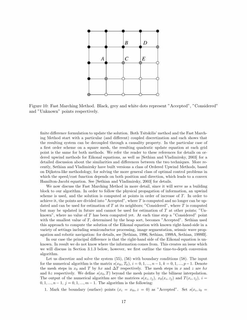
Figure 10: Fast Marching Method. Black, grey and white dots represent ”Accepted”, ”Considered”and ”Unknown” points respectively.

finite difference formulation to update the solution. Both Tsitskilis’ method and the Fast March-ing Method start with a particular (and different) coupled discretization and each shows thatthe resulting system can be decoupled through a causality property. In the particular case ofa first order scheme on a square mesh, the resulting quadratic update equation at each gridpoint is the same for both methods. We refer the reader to these references for details on or-dered upwind methods for Eikonal equations, as well as [Sethian and Vladimirsky, 2003] for adetailed discussion about the similarities and differences between the two techniques. More re-cently, Sethian and Vladimirsky have built versions a class of Ordered Upwind Methods, basedon Dijkstra-like methodology, for solving the more general class of optimal control problems inwhich the speed/cost function depends on both position and direction, which leads to a convexHamilton-Jacobi equation. See [Sethian and Vladimirsky, 2003] for details.

We now discuss the Fast Marching Method in more detail, since it will serve as a buildingblock to our algorithm. In order to follow the physical propagation of information, an upwindscheme is used, and the solution is computed at points in order of increase of T . In order toachieve it, the points are divided into ”Accepted”, where T is computed and no longer can be up-dated and can be used for estimation of T at its neighbors; ”Considered”, where T is computedbut may be updated in future and cannot be used for estimation of T at other points; ”Un-known”, where no value of T has been computed yet. At each time step a ”Considered” pointwith the smallest value of T , determined by the heap sort, becomes ”Accepted”. Sethian usedthis approach to compute the solution of the Eikonal equation with known right-hand-side in avariety of settings including semiconductor processing, image segmentation, seismic wave prop-agation and robotic navigation: for details, see [Sethian, 1996, Sethian, 1999A, Sethian, 1999B].

In our case the principal difference is that the right-hand side of the Eikonal equation is un-known. In result we do not know where the information comes from. This creates an issue whichwe will discuss in Section 3.1.3 below, however, we first outline the time-to-depth conversionalgorithm.

Let us discretize and solve the system (55), (56) with boundary conditions (58). The inputfor the numerical algorithm is the matrix s(x0i, Tk), i = 0, 1, ..., n− 1, k = 0, 1, ..., p− 1. Denotethe mesh steps in x0 and T by hx and ∆T respectively. The mesh steps in x and z are hxand hz respectively. We define s(x0, T ) beyond the mesh points by the bilinear interpolation.The output of the numerical algorithm are the matrices s(xi, zj), x0(xi, zj) and T (xi, zj), i =0, 1, ..., n− 1, j = 0, 1, ...,m− 1. The algorithm is the following:

1. Mark the boundary (surface) points (xi = x0i, z = 0) as ”Accepted”. Set s(xi, z0 =

17

0) = s(x0 = xi, T = 0), x0(x, z = 0) = x0, T (x, z = 0) = 0 according to the boundaryconditions. Mark the rest of the mesh points (xi, zj) as “Unknown”.

2. Mark the ”Unknown”points adjacent to the ”Accepted” points as ”Considered”. We calltwo points adjacent (or nearest neighbors) if they are separated by one edge.

3. Compute or update tentative values of s(xi, zj), x0(xi, zj) and T (xi, zj) at the ”Consid-ered” points.

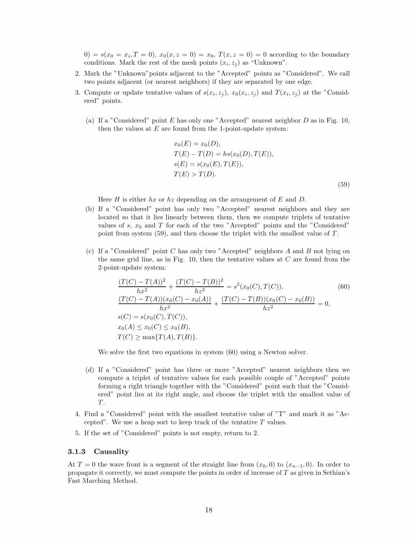
(a) If a ”Considered” point E has only one ”Accepted” nearest neighbor D as in Fig. 10,then the values at E are found from the 1-point-update system:

x0(E) = x0(D),

T (E) − T (D) = hs(x0(D), T (E)),

s(E) = s(x0(E), T (E)),

T (E) > T (D).

(59)

Here H is either hx or hz depending on the arrangement of E and D.

(b) If a ”Considered” point has only two ”Accepted” nearest neighbors and they arelocated so that it lies linearly between them, then we compute triplets of tentativevalues of s, x0 and T for each of the two ”Accepted” points and the ”Considered”point from system (59), and then choose the triplet with the smallest value of T .

(c) If a ”Considered” point C has only two ”Accepted” neighbors A and B not lying onthe same grid line, as in Fig. 10, then the tentative values at C are found from the2-point-update system:

(T (C) − T (A))2

hx2+

(T (C) − T (B))2

hz2= s2(x0(C), T (C)), (60)

(T (C) − T (A))(x0(C) − x0(A))

hx2+

(T (C) − T (B))(x0(C) − x0(B))

hz2= 0,

s(C) = s(x0(C), T (C)),

x0(A) ≤ x0(C) ≤ x0(B),

T (C) ≥ max{T (A), T (B)}.

We solve the first two equations in system (60) using a Newton solver.

(d) If a ”Considered” point has three or more ”Accepted” nearest neighbors then wecompute a triplet of tentative values for each possible couple of ”Accepted” pointsforming a right triangle together with the ”Considered” point such that the ”Consid-ered” point lies at its right angle, and choose the triplet with the smallest value ofT .

4. Find a ”Considered” point with the smallest tentative value of ”T” and mark it as ”Ac-cepted”. We use a heap sort to keep track of the tentative T values.

5. If the set of ”Considered” points is not empty, return to 2.

3.1.3 Causality

At T = 0 the wave front is a segment of the straight line from (x0, 0) to (xn−1, 0). In order topropagate it correctly, we must compute the points in order of increase of T as given in Sethian’sFast Marching Method.

18

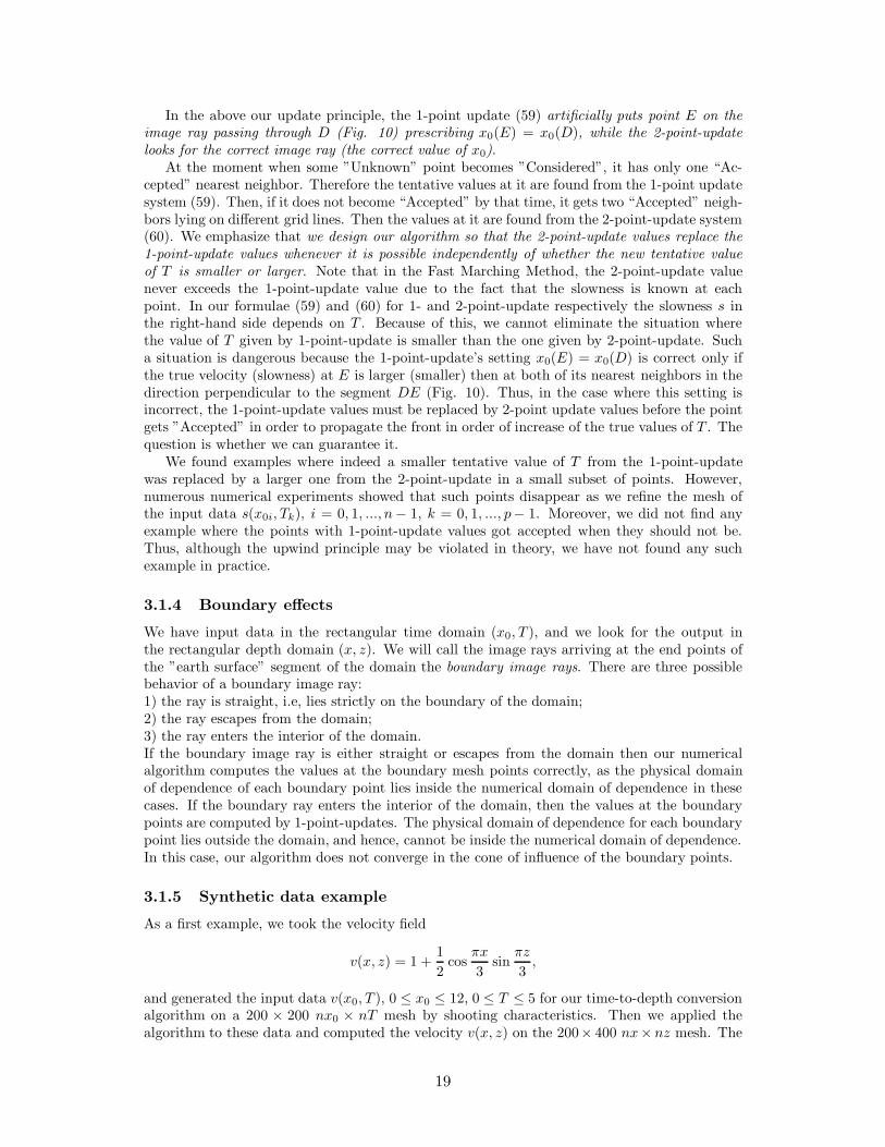
In the above our update principle, the 1-point update (59) artificially puts point E on theimage ray passing through D (Fig. 10) prescribing x0(E) = x0(D), while the 2-point-updatelooks for the correct image ray (the correct value of x0).

At the moment when some ”Unknown” point becomes ”Considered”, it has only one “Ac-cepted” nearest neighbor. Therefore the tentative values at it are found from the 1-point updatesystem (59). Then, if it does not become “Accepted” by that time, it gets two “Accepted” neigh-bors lying on different grid lines. Then the values at it are found from the 2-point-update system(60). We emphasize that we design our algorithm so that the 2-point-update values replace the1-point-update values whenever it is possible independently of whether the new tentative valueof T is smaller or larger. Note that in the Fast Marching Method, the 2-point-update valuenever exceeds the 1-point-update value due to the fact that the slowness is known at eachpoint. In our formulae (59) and (60) for 1- and 2-point-update respectively the slowness s inthe right-hand side depends on T . Because of this, we cannot eliminate the situation wherethe value of T given by 1-point-update is smaller than the one given by 2-point-update. Sucha situation is dangerous because the 1-point-update’s setting x0(E) = x0(D) is correct only ifthe true velocity (slowness) at E is larger (smaller) then at both of its nearest neighbors in thedirection perpendicular to the segment DE (Fig. 10). Thus, in the case where this setting isincorrect, the 1-point-update values must be replaced by 2-point update values before the pointgets ”Accepted” in order to propagate the front in order of increase of the true values of T . Thequestion is whether we can guarantee it.

We found examples where indeed a smaller tentative value of T from the 1-point-updatewas replaced by a larger one from the 2-point-update in a small subset of points. However,numerous numerical experiments showed that such points disappear as we refine the mesh ofthe input data s(x0i, Tk), i = 0, 1, ..., n− 1, k = 0, 1, ..., p− 1. Moreover, we did not find anyexample where the points with 1-point-update values got accepted when they should not be.Thus, although the upwind principle may be violated in theory, we have not found any suchexample in practice.

3.1.4 Boundary effects

We have input data in the rectangular time domain (x0, T ), and we look for the output inthe rectangular depth domain (x, z). We will call the image rays arriving at the end points ofthe ”earth surface” segment of the domain the boundary image rays. There are three possiblebehavior of a boundary image ray:1) the ray is straight, i.e, lies strictly on the boundary of the domain;2) the ray escapes from the domain;3) the ray enters the interior of the domain.If the boundary image ray is either straight or escapes from the domain then our numericalalgorithm computes the values at the boundary mesh points correctly, as the physical domainof dependence of each boundary point lies inside the numerical domain of dependence in thesecases. If the boundary ray enters the interior of the domain, then the values at the boundarypoints are computed by 1-point-updates. The physical domain of dependence for each boundarypoint lies outside the domain, and hence, cannot be inside the numerical domain of dependence.In this case, our algorithm does not converge in the cone of influence of the boundary points.

3.1.5 Synthetic data example

As a first example, we took the velocity field

v(x, z) = 1 +1

2cos

πx

3sin

πz

3,

and generated the input data v(x0, T ), 0 ≤ x0 ≤ 12, 0 ≤ T ≤ 5 for our time-to-depth conversionalgorithm on a 200 × 200 nx0 × nT mesh by shooting characteristics. Then we applied thealgorithm to these data and computed the velocity v(x, z) on the 200× 400 nx× nz mesh. The

19

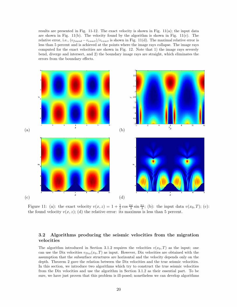
results are presented in Fig. 11-12. The exact velocity is shown in Fig. 11(a); the input dataare shown in Fig. 11(b). The velocity found by the algorithm is shown in Fig. 11(c). Therelative error, i.e., (vfound − vexact)/vexact is shown in Fig. 11(d). The maximal relative error isless than 5 percent and is achieved at the points where the image rays collapse. The image rayscomputed for the exact velocities are shown in Fig. 12. Note that 1) the image rays severelybend, diverge and intersect, and 2) the boundary image rays are straight, which eliminates theerrors from the boundary effects.

(a) (b)

(c) (d)

Figure 11: (a): the exact velocity v(x, z) = 1 + 1

2cos πx

3sin πz

3; (b): the input data v(x0, T ); (c):

the found velocity v(x, z); (d) the relative error: its maximus is less than 5 percent.

3.2 Algorithms producing the seismic velocities from the migration

velocities

The algorithm introduced in Section 3.1.2 requires the velocities v(x0, T ) as the input; onecan use the Dix velocities vDix(x0, T ) as input. However, Dix velocities are obtained with theassumption that the subsurface structures are horizontal and the velocity depends only on thedepth. Theorem 2 gave the relation between the Dix velocities and the true seismic velocities.In this section, we introduce two algorithms which try to construct the true seismic velocitiesfrom the Dix velocities and use the algorithm in Section 3.1.2 as their essential part. To besure, we have just proven that this problem is ill-posed; nonetheless we can develop algorithms

20

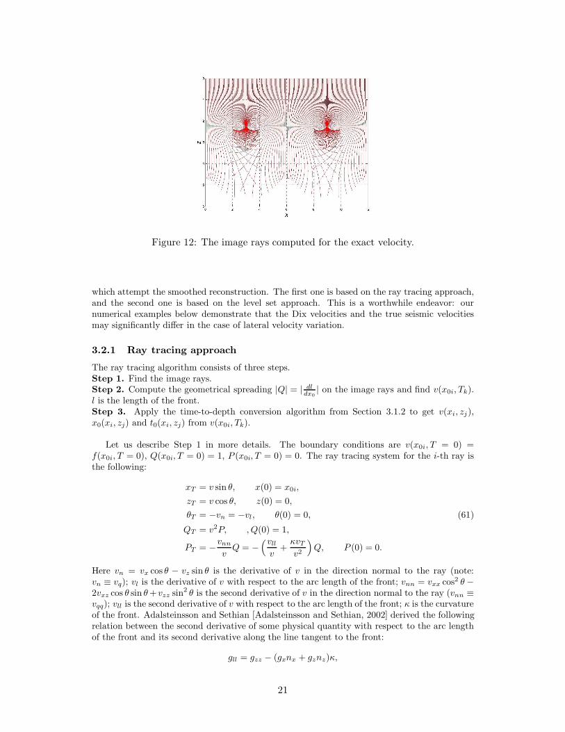
Figure 12: The image rays computed for the exact velocity.

which attempt the smoothed reconstruction. The first one is based on the ray tracing approach,and the second one is based on the level set approach. This is a worthwhile endeavor: ournumerical examples below demonstrate that the Dix velocities and the true seismic velocitiesmay significantly differ in the case of lateral velocity variation.

3.2.1 Ray tracing approach

The ray tracing algorithm consists of three steps.Step 1. Find the image rays.Step 2. Compute the geometrical spreading |Q| = | dl

dx0

| on the image rays and find v(x0i, Tk).l is the length of the front.Step 3. Apply the time-to-depth conversion algorithm from Section 3.1.2 to get v(xi, zj),x0(xi, zj) and t0(xi, zj) from v(x0i, Tk).

Let us describe Step 1 in more details. The boundary conditions are v(x0i, T = 0) =f(x0i, T = 0), Q(x0i, T = 0) = 1, P (x0i, T = 0) = 0. The ray tracing system for the i-th ray isthe following:

xT = v sin θ, x(0) = x0i,

zT = v cos θ, z(0) = 0,

θT = −vn = −vl, θ(0) = 0, (61)

QT = v2P, , Q(0) = 1,

PT = −vnn

vQ = −

(vll

v+

κvT

v2

)

Q, P (0) = 0.

Here vn = vx cos θ − vz sin θ is the derivative of v in the direction normal to the ray (note:vn ≡ vq); vl is the derivative of v with respect to the arc length of the front; vnn = vxx cos2 θ −2vxz cos θ sin θ +vzz sin2 θ is the second derivative of v in the direction normal to the ray (vnn ≡vqq); vll is the second derivative of v with respect to the arc length of the front; κ is the curvatureof the front. Adalsteinsson and Sethian [Adalsteinsson and Sethian, 2002] derived the followingrelation between the second derivative of some physical quantity with respect to the arc lengthof the front and its second derivative along the line tangent to the front:

gll = gzz − (gxnx + gznz)κ,

21

where n is the unit vector normal to the front. Replacing g with v and noticing that

vxnx + vznz = vτ =vT

v

is the derivative of v with respect to the arc length of the ray, we get the last equation in (61).We solve system (61) for all of the rays simultaneously by the forward Euler method as

follows.For k = 0 to k = p − 1 do:

1. Find the least squares polynomials for the set of points (li, vi(Tk)) where li is the arc lengthof the front between ray 0 and ray i at the time Tk, and vi(Tk) is the value of the velocityon the i-th ray at time Tk. Evaluate vl(Tk) and vll(Tk) taking the first and the secondderivatives of this polynomial. Moreover, replace the values of the velocity vi(Tk) by thevalues of this polynomial. Evaluate the curvature κ(Tk) as follows. Find the least squarespolynomials for the sets of points (i, xi(Tk)) and (i, zi(Tk)) where i is the index of the ray,and xi and zi are the x- and z-coordinates of the i-th ray at time Tk. Take the first andthe second derivatives of these polynomials px and pz and find

κ =p′xp′′z − p′zp

′′x

(p′2x + p′2z )3/2.

Approximate vT (Tk) by

vt(Tk) =v(Tk) − v(Tk−1)

∆T

if k > 0, and we set vT (T0 = 0) = 0, since the curvature of the front is zero at T = 0.

2. Perform one forward Euler step for each of the rays.

3. For each of the rays find vi(Tk+1) = fi(Tk+1)Q(Tk+1), where fi(tk+1) ≡ f(x0i, Tk+1),i = 0, 1, ..., n− 1.

Remarks.

• One can see that we find v(x0i, Tk), i = 0, 1, ..., n − 1, k = 0, 1, ..., p − 1 in the step1. Hence it is possible immediately go to step 3 to find v(xi, zj). However, numerousnumerical experiments showed that step 1 computes the image rays (x(x0i, Tk), z(x0i, Tk))significantly more accurately than the velocity v(x0i, Tk). And Step 2 which is very simple,significantly improves the accuracy of v(x0i, Tk).

• As we have shown in Section 2.6 the inverse problem is numerically unstable. The use ofthe least squares polynomials suppresses the growth of the small bumps which naturallyappear in result of computations, and hence, stabilizes the algorithm.

• The main limitation of this algorithm is that it blows up as the image rays come too closeto each other or diverge too much.

• One can use the additional output x0(xi, zj) and t0(xi, zj) to convert a time-migratedimage to depth rather than perform depth migration with the found velocities v(xi, zj).

3.2.2 Level set approach

Level set methods, introduced in Osher and Sethian [Osher and Sethian, 1988], are numericalmethods for tracking moving interfaces: they rely in part on the theory of curve and surfaceevolution given in Sethian [Sethian, 1982, Sethian, 1985] and on the link between front propa-gation and hyperbolic conservation laws discussed in Sethian [Sethian, 1987]. These techniquesrecast interface motion as a time-dependent Eulerian initial value partial differential equation.For a general introduction and overview, see Sethian [Sethian, 1999B].

The main idea of a level set method is the representation of a front as the zero level setof some higher dimensional function. In our context, we want to propagate the wave frontcoinciding with the flat surface at t = 0 downward the earth. We embed the wave front into a

22

2D function φ(x, z) so that the front is its zero level set. Furthermore, we embed the quantitiesQ and P defined on the front into 2D functions q(x, z) and p(x, z) so that at each moment oftime Q = q(x, z){(x,z)|φ(x,z)=0} and P = p(x, z){(x,z)|φ(x,z)=0}, i.e., Q and P coincide with q andp on the zero level set of φ(x, z). Let

gx =φx

|∇φ|, gz =φz

|∇φ|.

Let us find the system of equations for q and p. First note that

vnn = vxx cos2 θ − 2vxz cos θ sin θ + vzz sin2 θ.

Second, at each point of the the zero level set of φ, i.e. at each front point,

gx = cos θ, gz = sin θ.

Then we get the following equations for q and p:

qt = v2p, pt = −vxxg2x − 2vxzgxgz + vzzg

2z

vq. (62)

These equations coincide with the equations for Q and P on the front. Here we switch thenotation for time from T to t. We will reserve the notation T for auxiliary times in the fastmarching parts of our level set algorithm.

Thus, we have to solve the following system of PDE’s:

φt + v(x, z)|∇φ| = 0,

qt = v2(x, z)p, (63)

pt = −vxxg2x − 2vxzgxgz + vzzg

2z

v(x, z)q.

As before, we have the input data f(x0 , t) = v(x0,t)|Q(x0,t)| given in (x0, t) space on a n× k mesh,

and we need to obtain v(x, z) in (x, z) space on a n × m mesh.Initialization: Set q(x, z) = 1, p(x, z) = 0, which is correct for the front at t = 0. Set

v(x, 0) = f(x0, 0) and attach labels ”x” to the surface points. Set φ(x, z) = z, i.e., make thelevel set function a signed distance function.

We solve system (63) in the following time cycle: for k = 0 to p − 1 do:

1. Starting with the current ”x” points, solve the system

q(x, z)|∇T | = 1

f(x0, T ), ∇x0 · ∇T = 0

using the Fast Marching time-to-depth conversion algorithm introduced in Section 3.1.2to find v(x, z) = f(x, z)q(x, z) for the current q(x, z).

2. Attach labels ”x” to the accepted points for which T is not greater than the current valueof time tk.

3. Detect the zero level set of φ. Find the velocity v at the zero level set of φ and build anextension of v solving the system

|∇d| = 1, ∇d · ∇vext = 0,

with the boundary conditions d = 0 and vext = v at the zero level set of φ, using the FastMarching Method, as it is suggested in [Sethian, 1996, Sethian, 1999A]. If the extendedvelocity is built this way, φ remains to be the signed distance function if it was it at t = 0.

23

4. Perform a time step: Compute the quantities gx and gz for the current φ. Find vxx, vxz

and vzz by finding least square polynomials for each grid line x = xi and z = zj andevaluating their derivatives. Make one forward Euler step for equations (62) to find new qand p. Solve the level set equation

φt + vext|∇φ| = 0

from t = k∆t to t = (k + 1)∆t by the forward Euler method with a time step satisfyingthe CFL condition.

The main advantage of this algorithm in comparison with the ray tracing algorithm is thatit can work even if the image rays intersect, since it tracks the first arrival front.

Having obtained the true seismic velocities v(xi, zj) one can perform depth migration toobtain an improved seismic image in the Cartesian coordinates. Alternatively, knowing the ve-locity v(xi, zj) one can apply Sethian’s fast marching method [Sethian, 1996] to obtain t0(xi, zi)and x0(xi, zi) to convert the time migrated image to depth.

4 Synthetic data examples

4.1 Example 1

The example in this section allows us to compare performances of the ray tracing algorithm andlevel set algorithm with a somewhat typical approach. One typical approach to seismic velocityestimation is to compute the Dix velocities and then apply image ray tracing. Here we willreplace the image ray tracing with our time-to-depth conversion algorithm.

We considered the velocity fields of the form:

v(x, z) = 1 + exp(

−c(x2 + (z − 1)2))

, x0 ∈ [−2, 2], t ∈ [0, 0.7]. (64)

We took c = 0.5, c = 1 and c = 1.5. The larger c, the sharper the Gaussian anomaly. For eachof these fields we created the input data f(x0 , t) on a 200× 200 x0 × t mesh and applied each ofthe three algorithms to them: the time-to-depth conversion, the ray tracing, and the level set.The output v(x, z) is given on 200× 200 x × z mesh.

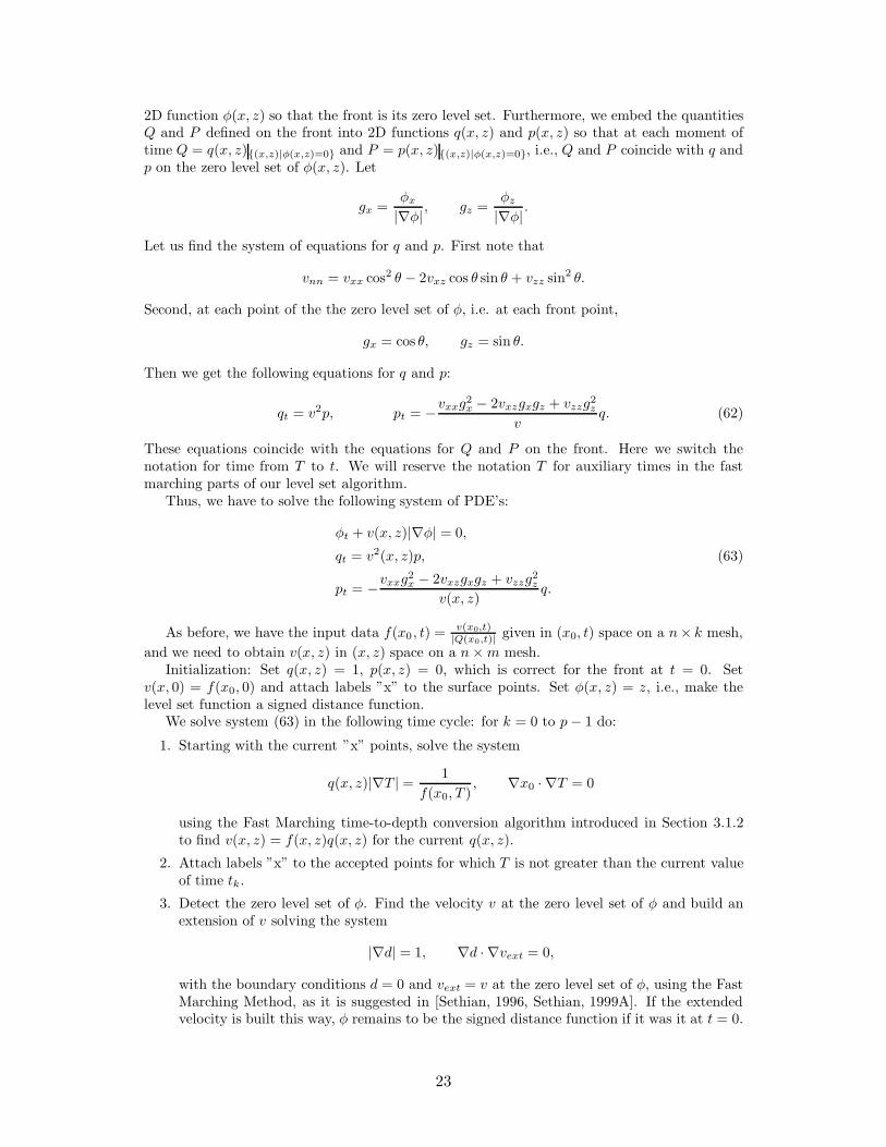
The exact velocity, the input data (the Dix velocity, the found velocity and the image raysfor the sharpest Gaussian anomaly corresponding c = 1.5 are shown in Fig. 13. We see that theDix velocity qualitatively differs from the exact velocity and the found velocity resembles theexact velocity much more than the Dix velocity.

The results are summarized in Table (1). We see that

Table 1: The maximal relative errors produced by the time-to-depth conversion, the ray tracing

and the level set algorithms on the data from the velocity field (64).

Algorithm Time-to-depth Ray tracing Level set

c = 0.5 0.31 0.023 0.078

c = 1 0.44 0.11 0.079

c = 1.5 0.49 0.29 0.20

• the ray tracing and the level set produce significantly more accurate results than the typicalapproach;

• the ray tracing approach is more accurate than the level set where the image rays divergemoderately, while it becomes less accurate as the divergence of the image rays increases.

Note that if the image rays diverge severely so that the derivative vnn (or, in different notations,vqq) becomes large, both our ray tracing and level set algorithms blow up, while the time-to-depth convergence algorithm produces inaccurate but stable results.

24

(a) (b)

(c) (d)

Figure 13: (a): the exact velocity v(x, z); (b): the input data f(x0, t) ≡ vDix(x0, t); (c): the found

velocity v(x, z); (d) the image rays.

4.2 Example 2

In this section we also consider an example with a Gaussian anomaly, but with numbers closerto the real seismic numbers:

v(x, z) = 2 + 2 exp(

−(x2 + (z − 2)2))

,

x0 ∈ [−3, 3], t ∈ [0, 1],

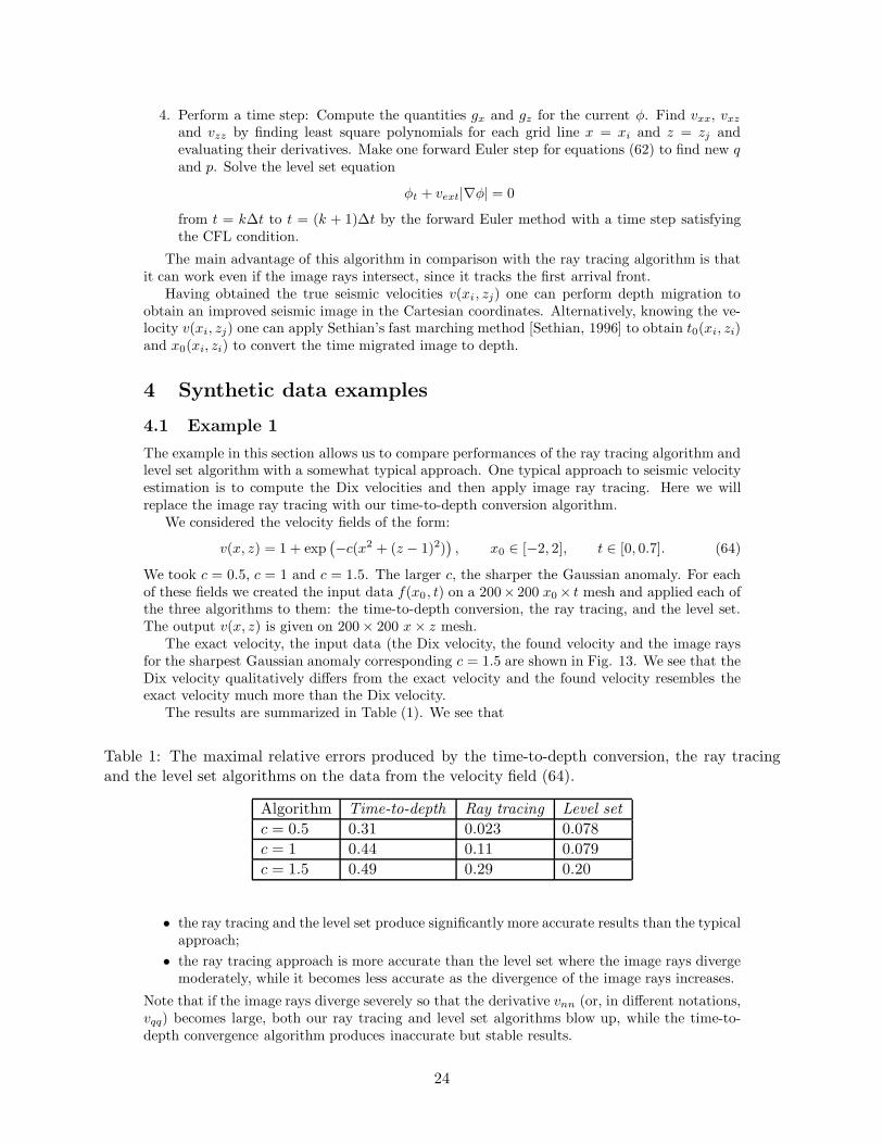
The center of the anomaly lies at the depth of 2 km and the background velocity is 2 km/sec.The results (Fig. 14) are produced by the level set algorithm. The found velocity resembles theexact velocity while the Dix velocity and the found velocity differ qualitatively.

5 Field data example

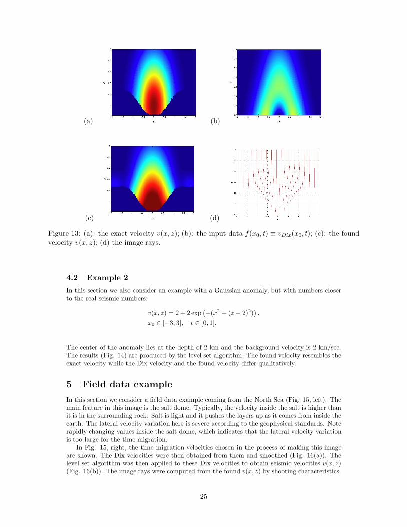
In this section we consider a field data example coming from the North Sea (Fig. 15, left). Themain feature in this image is the salt dome. Typically, the velocity inside the salt is higher thanit is in the surrounding rock. Salt is light and it pushes the layers up as it comes from inside theearth. The lateral velocity variation here is severe according to the geophysical standards. Noterapidly changing values inside the salt dome, which indicates that the lateral velocity variationis too large for the time migration.

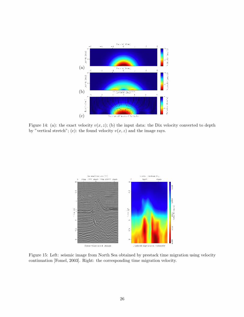
In Fig. 15, right, the time migration velocities chosen in the process of making this imageare shown. The Dix velocities were then obtained from them and smoothed (Fig. 16(a)). Thelevel set algorithm was then applied to these Dix velocities to obtain seismic velocities v(x, z)(Fig. 16(b)). The image rays were computed from the found v(x, z) by shooting characteristics.

25

(a)

(b)

(c)

Figure 14: (a): the exact velocity v(x, z); (b) the input data: the Dix velocity converted to depth

by ”vertical stretch”; (c): the found velocity v(x, z) and the image rays.

Figure 15: Left: seismic image from North Sea obtained by prestack time migration using velocity

continuation [Fomel, 2003]. Right: the corresponding time migration velocity.

26

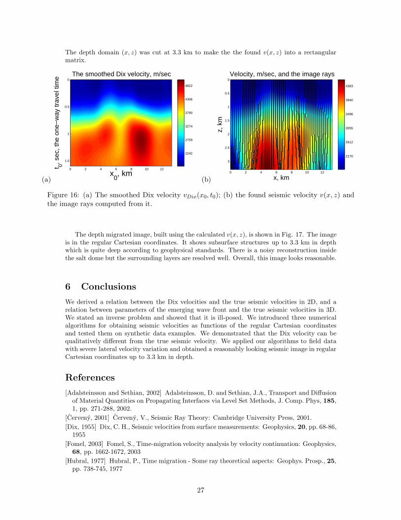
The depth domain (x, z) was cut at 3.3 km to make the the found v(x, z) into a rectangularmatrix.

(a)x

0, km

t 0, sec

, the

one

−w

ay tr

avel

tim

e

The smoothed Dix velocity, m/sec

0 2 4 6 8 10 12

0

0.5

1

1.5

2242

2759

3274

3790

4306

4822

(b) x, km

z, k

m

Velocity, m/sec, and the image rays

0 2 4 6 8 10 12

0

0.5

1

1.5

2

2.5

3

2170

2612

3055

3496

3840

4383

Figure 16: (a) The smoothed Dix velocity vDix(x0, t0); (b) the found seismic velocity v(x, z) andthe image rays computed from it.

The depth migrated image, built using the calculated v(x, z), is shown in Fig. 17. The imageis in the regular Cartesian coordinates. It shows subsurface structures up to 3.3 km in depthwhich is quite deep according to geophysical standards. There is a noisy reconstruction insidethe salt dome but the surrounding layers are resolved well. Overall, this image looks reasonable.

6 Conclusions

We derived a relation between the Dix velocities and the true seismic velocities in 2D, and arelation between parameters of the emerging wave front and the true seismic velocities in 3D.We stated an inverse problem and showed that it is ill-posed. We introduced three numericalalgorithms for obtaining seismic velocities as functions of the regular Cartesian coordinatesand tested them on synthetic data examples. We demonstrated that the Dix velocity can bequalitatively different from the true seismic velocity. We applied our algorithms to field datawith severe lateral velocity variation and obtained a reasonably looking seismic image in regularCartesian coordinates up to 3.3 km in depth.

References

[Adalsteinsson and Sethian, 2002] Adalsteinsson, D. and Sethian, J.A., Transport and Diffusionof Material Quantities on Propagating Interfaces via Level Set Methods, J. Comp. Phys, 185,1, pp. 271-288, 2002.

[Cerveny, 2001] Cerveny, V., Seismic Ray Theory: Cambridge University Press, 2001.

[Dix, 1955] Dix, C. H., Seismic velocities from surface measurements: Geophysics, 20, pp. 68-86,1955

[Fomel, 2003] Fomel, S., Time-migration velocity analysis by velocity continuation: Geophysics,68, pp. 1662-1672, 2003

[Hubral, 1977] Hubral, P., Time migration - Some ray theoretical aspects: Geophys. Prosp., 25,pp. 738-745, 1977

27

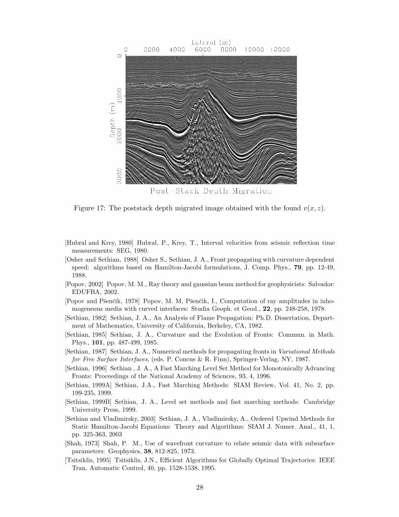
Figure 17: The poststack depth migrated image obtained with the found v(x, z).

[Hubral and Krey, 1980] Hubral, P., Krey, T., Interval velocities from seismic reflection timemeasurements: SEG, 1980.

[Osher and Sethian, 1988] Osher S., Sethian, J. A., Front propagating with curvature dependentspeed: algorithms based on Hamilton-Jacobi formulations, J. Comp. Phys., 79, pp. 12-49,1988.

[Popov, 2002] Popov, M. M., Ray theory and gaussian beam method for geophysicists: Salvador:EDUFBA, 2002.

[Popov and Psencik, 1978] Popov, M. M, Psencik, I., Computation of ray amplitudes in inho-mogeneous media with curved interfaces: Studia Geoph. et Geod., 22, pp. 248-258, 1978.

[Sethian, 1982] Sethian, J. A., An Analysis of Flame Propagation: Ph.D. Dissertation, Depart-ment of Mathematics, University of California, Berkeley, CA, 1982.

[Sethian, 1985] Sethian, J. A., Curvature and the Evolution of Fronts: Commun. in Math.Phys., 101, pp. 487-499, 1985.

[Sethian, 1987] Sethian, J. A., Numerical methods for propagating fronts in Variational Methodsfor Free Surface Interfaces, (eds. P. Concus & R. Finn), Springer-Verlag, NY, 1987.

[Sethian, 1996] Sethian , J. A., A Fast Marching Level Set Method for Monotonically AdvancingFronts: Proceedings of the National Academy of Sciences, 93, 4, 1996.

[Sethian, 1999A] Sethian, J.A., Fast Marching Methods: SIAM Review, Vol. 41, No. 2, pp.199-235, 1999.

[Sethian, 1999B] Sethian, J. A., Level set methods and fast marching methods: CambridgeUniversity Press, 1999.

[Sethian and Vladimirsky, 2003] Sethian, J. A., Vladimirsky, A., Ordered Upwind Methods forStatic Hamilton-Jacobi Equations: Theory and Algorithms: SIAM J. Numer. Anal., 41, 1,pp. 325-363, 2003

[Shah, 1973] Shah, P. M., Use of wavefront curvature to relate seismic data with subsurfaceparameters: Geophysics, 38, 812-825, 1973.

[Tsitsiklis, 1995] Tsitsiklis, J.N., Efficient Algorithms for Globally Optimal Trajectories: IEEETran. Automatic Control, 40, pp. 1528-1538, 1995.

28

[Yilmaz, 2001] Yilmaz, O., Seismic Data Analysis: Soc. of Expl. Geophys., 2001

29