Seismic Shot Processing on GPU - NTNU · 2009-08-25 · Seismic processing applications typically...

June 2009Anne Cathrine Elster, IDIJohn Hybertsen, StatoilHydro

Master of Science in Computer ScienceSubmission date:Supervisor:Co-supervisor:

Norwegian University of Science and TechnologyDepartment of Computer and Information Science

Seismic Shot Processing on GPU

Owe Johansen

Problem DescriptionSeismic processing applications typically process large amounts of data and are verycomputationally demanding. A wide variety of high performance applications have recently beenmodified to use GPU devices for off-loading their computational workload, often with considerableperformance improvements.

In this project, we will in collaborations with StatoilHydro, explore how a seismic application usedfor handling shot data on large clusters, can take advantage of GPU technoligies. The project mayinclude looking at relevant GPU libraries and compilers as well as considering porting relevantlibrary components currently provided by the StatiliHydro application enviroment.

Performance comparison with the original codes will be included, as well as an evaluation of thedevelopement effort required for implementing such techniques.

Assignment given: 23. January 2009Supervisor: Anne Cathrine Elster, IDI

Abstract

Today’s petroleum industry demand an ever increasing amount of compu-tational resources. Seismic processing applications in use by these types ofcompanies have generally been using large clusters of compute nodes, whoseonly computing resource has been the CPU. However, using Graphics Pro-cessing Units (GPU) for general purpose programming is these days becomingincreasingly more popular in the high performance computing area. In 2007,NVIDIA corporation launched their framework for developing GPU utilizingcomputational algorithms, known as the Compute Unied Device Architec-ture (CUDA), a wide variety of research areas have adopted this frameworkfor their algorithms. This thesis looks at the applicability of GPU techniquesand CUDA for off-loading some of the computational workload in a seismicshot modeling application provided by StatoilHydro to modern GPUs.

This work builds on our recent project that looked at providing check-point restart for this MPI enabled shot modeling application. In this thesis,we demonstrate that the inherent data parallelism in the core finite-differencecomputations also makes our application well suited for GPU acceleration.By using CUDA, we show that we could do an efficient port our application,and through further refinements achieve significant performance increases.

Benchmarks done on two different systems in the NTNU IDI (Depart-ment of Computer and Information Science) HPC-lab, are included. Onesystem is a Intel Core2 Quad Q9550 @2.83GHz with 4GB of RAM andan NVIDIA GeForce GTX280 and NVIDIA Tesla C1060 GPU. Our sec-ond testbed was an Intel Core I7 Extreme (965 @3.20GHz) with 12GB ofRAM hosting an NVIDIA Tesla S1070 (4X NVIDIA Tesla C1060). On thishardware, speedups up to a factor of 8-14.79 compared to the original se-quential code are achieved, confirming the potential of GPU computing inapplications similar to the one used in this thesis.

Problem Description

Seismic processing applications typically process large amounts of data andare very computationally demanding. A wide variety of high performanceapplications have recently been modified to use GPU devices for off-loadingtheir computational workload, often with considerable performance improve-ments.

In this project, we will in collaborations with StatoilHydro, explore howa seismic application used for handling shot data on large clusters, can takeadvantage of GPU technologies.

The project may include looking at relevant GPU libraries and compilersas well as considering porting relevant library components currently providedby the StatoilHydro application environment. Performance comparison withthe original codes will be included, as well as an evaluation of the developmenteffort required for implementing such techniques.

I

Acknowledgments

There have been several people involved with making the work in this thesispossible. Here, I would like to especially thank the following:

• Dr. Anne Cathrine Elster, who has been my main thesis advisor at theNorwegian University of Science and Technology (NTNU). Dr. Elsterhas helped getting the project approved, and has also given valuableadvice during the course of the work.

• StatoilHydro, for supplying the application subject to this thesis, aswell as the data sets used.

• John Hybertsen of StatoilHydro. Mr. Hybertsen helped define theproblem of this thesis, and has also been a very positive influence bysupporting the work.

• Jon Andre Haugen of StatoilHydro. Mr. Haugen is one of the chiefdevelopers of the application subject to the work in this thesis. Hishelp with explaining the finer points of the application, especially thegeophysical aspects, as well has his feedback on this work, has beeninvaluable.

• Dr. Joachim Mispel of StatoilHydro. Dr. Mispel, also one of the Chiefdevelopers of the library (SPL) which the application in this thesis isbased on, has been very helpful by giving useful comments on this work,as well as participating in clarifying discussions.

II

Contents

1 Introduction 11.1 Our Targeted Seismic Application . . . . . . . . . . . . . . . . 11.2 Project Goals . . . . . . . . . . . . . . . . . . . . . . . . . . . 21.3 Outline . . . . . . . . . . . . . . . . . . . . . . . . . . . . . . . 2

2 Seismic Shot Processing 42.1 Marine Seismic Acquisition . . . . . . . . . . . . . . . . . . . . 42.2 Application Details . . . . . . . . . . . . . . . . . . . . . . . . 5

3 GPU Programming & FDM 93.1 GPU Programming . . . . . . . . . . . . . . . . . . . . . . . . 93.2 CUDA . . . . . . . . . . . . . . . . . . . . . . . . . . . . . . . 143.3 The Finite Difference Method (FDM) . . . . . . . . . . . . . . 193.4 Related Work on CUDA GPU Offloading . . . . . . . . . . . . 21

4 Application Analysis and Optimization 234.1 Profiling and Analysis . . . . . . . . . . . . . . . . . . . . . . 234.2 Implementing GPU Offloading . . . . . . . . . . . . . . . . . . 27

4.2.1 First Implementation . . . . . . . . . . . . . . . . . . . 284.2.2 Second Implementation . . . . . . . . . . . . . . . . . . 304.2.3 Third Implementation . . . . . . . . . . . . . . . . . . 32

4.3 Multi GPU . . . . . . . . . . . . . . . . . . . . . . . . . . . . 34

5 Results & Discussion 365.1 Methodology . . . . . . . . . . . . . . . . . . . . . . . . . . . 365.2 Test Systems . . . . . . . . . . . . . . . . . . . . . . . . . . . 375.3 Benchmark Results . . . . . . . . . . . . . . . . . . . . . . . . 37

5.3.1 Results from the HPC workstations . . . . . . . . . . . 37

III

CONTENTS IV

5.3.2 Scaling Characteristics . . . . . . . . . . . . . . . . . . 405.4 Discussion . . . . . . . . . . . . . . . . . . . . . . . . . . . . . 41

6 Conclusions & Future Work 436.1 Future Work . . . . . . . . . . . . . . . . . . . . . . . . . . . . 44

6.1.1 GPU Utilizing Mathematical Libraries . . . . . . . . . 446.1.2 Further Improvements to SplFd2dmod . . . . . . . . . 446.1.3 Further Testing . . . . . . . . . . . . . . . . . . . . . . 45

List of Figures

2.1 Seismic acquisition. The vessel in the Figure tows a streamerand air guns. The reflections of the pressure wave off interfacesin the sub surface are illustrated . . . . . . . . . . . . . . . . . 5

2.2 Application output after modeling a shot . . . . . . . . . . . . 62.3 Shot gathers containing 12 modeled shots . . . . . . . . . . . . 62.4 Flowchart for the application taken from [5]. The flow of the

slave processes is shown in the green rectangle. The red rect-angle shows the flow of the I/O server . . . . . . . . . . . . . . 7

3.1 Simplified view of a graphics pipeline with indication of streamsbetween the different stages as well as their memory accesses . 11

3.2 TPC of the GTX200 architecture. A GeForce GTX280 GPUcard contains a total of 10 TPCs. (With permission fromNVIDIA) . . . . . . . . . . . . . . . . . . . . . . . . . . . . . 15

3.3 Thread organization on GPU in terms of grids and blocks . . . 173.4 CUDA Memory Layout, Showing the different memory types . 193.5 Visualization of the centered difference approximation in Equa-

tion 3.8. Point computed is in green, while evaluated pointsare in red . . . . . . . . . . . . . . . . . . . . . . . . . . . . . 21

4.1 Function call path of our application obtained from the Call-Grind tool . . . . . . . . . . . . . . . . . . . . . . . . . . . . . 24

4.2 Problem domain with added PML layers . . . . . . . . . . . . 264.3 Modeling loop of the Fd2dModfd routine . . . . . . . . . . . . 264.4 Execution configuration superimposed on the total working

area of the model (compare with Figure 4.2) . . . . . . . . . . 284.5 Logical kernel assignment for the first implementation of the

Fd2dTimestep routine. See Figure 4.3 for reference . . . . . . 28

V

LIST OF FIGURES VI

4.6 Horizontal differentiator regions of computation . . . . . . . . 304.7 Shared memory region for thread blocks in the horizontal dif-

ferentiators . . . . . . . . . . . . . . . . . . . . . . . . . . . . 314.8 Shared memory region for thread blocks in the vertical differ-

entiators . . . . . . . . . . . . . . . . . . . . . . . . . . . . . . 314.9 Logical kernel assignment for the second implementation of

the Fd2dTimestep routine. See Figure 4.3 for reference . . . . 324.10 Logical kernel assignment for the third implementation of the

Fd2dTimestep routine. See Figure 4.3 for reference . . . . . . 334.11 Updated work flow for hybrid CPU/GPU implementation . . . 35

5.1 HPC lab 1 running NVIDIA GeForce GTX280 . . . . . . . . . 385.2 HPC lab 1 running NVIDIA Tesla C1060 . . . . . . . . . . . . 395.3 HPC lab 2 running single NVIDIA Tesla C1060 . . . . . . . . 395.4 CPU Scaling results with {1,2,3,4} processes . . . . . . . . . . 405.5 GPU Scaling results with {1,2,3,4} processes . . . . . . . . . . 41

Chapter 1

Introduction

Using Graphics Processing Units (GPU) for general purpose programmingis becoming increasingly popular in high performance computing (HPC).Since NVIDIA corporation in 2007 launched a framework for developingGPU utilizing computational algorithms, known as the Compute UnifiedDevice Architecture (CUDA), a wide variety of research areas have adoptedthis framework for their algorithms. Examples of research disciplines usingCUDA include computational biophysics, image and signal processing, geo-physical imaging, game physics, molecular dynamics and computational fluiddynamics (see e.g. [1], [2], [3] and [4]).

The massively parallel architecture of CUDA enabled GPU devices makesthem a perfect fit for algorithms which behave in a highly data parallel man-ner. Reported algorithm speedups in excess of 100x compared to conventionalCPU implementations, and relatively low cost, further motivates the use ofsuch hardware for computationally intensive algorithms.

1.1 Our Targeted Seismic Application

The work presented in this thesis continues the work we previously did in[5], where StatoilHydro provided us with a seismic shot modeling applica-tion and sample synthetic data. The application is MPI based for parallelexecution on the large production compute clusters at StatoilHydro. In [5],we implemented checkpoint/restart functionality, which guaranteed that allthe work assigned to the application would complete regardless of potentialsituations in which nodes of the compute cluster failed.

1

CHAPTER 1. INTRODUCTION 2

The main focus of the work presented in this thesis will be different com-pared to the previous work in that we here will attempt to improve theefficiency of the application by off-loading some of the numerical calculationsto the GPU, where as we previously focused on improving application con-sistency and fault tolerance. The application we worked on back then wasan earlier revision of the one used in this thesis.

1.2 Project Goals

In this project, we will in collaborations with StatoilHydro explore the po-tential of using CUDA based GPU offloading for improving the performanceof the provided seismic shot modeling application. The provided applicationis currently being used on a production compute cluster at StatoilHydro.

We will attempt to include a review of existing GPU enabled HPC li-braries and compilers, as well as consider porting library components of partsof the StatoilHydro application environment to GPU.

We will conduct performance comparisons of the developed GPU enabledapplication and the original, and finally evaluate the development effort re-quired for implementing the CUDA enabled GPU utilizing components.

1.3 Outline

The contents of this thesis is structered as follows:

• Chapter 2 introduces our application targeted for GPU computationaloffloading. It starts off by describing the fundamentals of marine seis-mic acquisition, and proceeds by describing the workings of our appli-cation, as well as how it relates to this principle.

• Chapter 3 will explore the details of GPU programming, in particularwith respect to NVIDIA’s CUDA framework. It will also review thebasics of the Finite Difference Method, as well as mention some ofthe works done in the field of GPU programming on applications withvarious algorithmic commonalities to our target application.

• Chapter 4 starts off with profiling a run of the original application,which is subsequently used to indicate which areas to target for GPUoffloading. Following the profiling results, the Chapter describes the

CHAPTER 1. INTRODUCTION 3

functionality of the selected target areas, and proceeds by detailingthe process of modifying them so that they take advantage of GPUdriven computational offloading. 3 GPU utilizing implementations willbe developed, with the last being the most optimal. The Chapterconcludes by describing the implementation of multiple GPU supportin the application.

• Chapter 5 contains performance measurements of the developed GPUimplementations. The Chapter starts off describing test methodologyand the test environment, followed by benchmarking results for all de-veloped GPU implementations, as well as the original. In the end, theresults obtained from the benchmarking are discussed.

• Chapter 6 concludes the work done in this thesis, and suggests somepossible alternatives for future work.

Chapter 2

Seismic Shot Processing

In this Chapter we will introduce the application in which we intend toimplement GPU computational offloading techniques. We will start off byintroducing the basics of seismic acquisition, and proceed by describing theworkings of our application and how it relates to this principle.

2.1 Marine Seismic Acquisition

Marine seismic acquisition (see Chapter 7 of [6]), is the process where a vessel(boat) releases pressure waves (shots) from an air gun (source) underneaththe sea surface. The vessel tows a cable (streamer) with listening devices(hydrophones). When the pressure wave from a shot reaches an interfacein the sub surface, some of its energy is reflected towards the surface. Thehydrophones of the streamer collects these reflections, or signals, which con-tain information about pressure changes in the water. Data collection fromthe streamers is commonly performed for several shots taken with increasingor decreasing distance between source and receiver (hydrophone), producingwhat is known as a seismic shot gather. An illustration of marine seismicacquisition is shown in Figure 2.1

4

CHAPTER 2. SEISMIC SHOT PROCESSING 5

Figure 2.1: Seismic acquisition. The vessel in the Figure tows a streamerand air guns. The reflections of the pressure wave off interfaces in the subsurface are illustrated

2.2 Application Details

Our application, SplFd2dmod, which is a part of StatoilHydro’s SeismicProcessing Library (SPL), simulates seismic shot data by means of finite dif-ference modeling. The data on which the application bases its modeling, aresynthetic velocity and density models of the sub surface which describe theacoustic impedance (interfaces/contrast) in the different areas of the model.SplFd2dmod computes a sub surface pressure field by propagating a pressurewave (shot) through the modeled area characterized by the aforementionedvelocity and density models. Figure 2.2 is an example output of modeling asingle shot gather, and Figure 2.3 is an example of several shot gathers. Con-trast in both of these Figures has been enhanced by discarding amplitudesoutside the range [−0.0001, 0.0001].


Figure 2.2: Application output aftermodeling a shot

Figure 2.3: Shot gathers containing 12modeled shots

The application has a single- and a multiprocessor (MPI) mode of exe-cution. The multi processor mode is built in an SPMD fashion, meaning itis written as a single program working on multiple data elements. The dataelements of the application are the seismic shot records. The application isparallelized by shot record, meaning each slave process on nodes of the com-putational cluster running it will process a single shot. The master process(rank 0) of the application works as an I/O server, with the intent of assur-ing atomic read/write access to files requested by the slave processes. Thisenforces consistency and minimizes file system pressure. FIO is the librarycomponent of SPL containing the I/O server.

The slave processes pick a seismic shot from a file containing all theavailable shots. The selection of shots is governed by a key-map file, keepingtrack of which shots are available and which are being/have been modeled.The key-map file is, as with the other input files, shared among all theprocesses.


Figure 2.4: Flowchart for the application taken from [5]. The flow of theslave processes is shown in the green rectangle. The red rectangle shows theflow of the I/O server

Each slave process does a 2D acoustic finite difference modeling of agiven shot, and outputs its result in a single shared file, which in the end willcontain all of the modeled shots. When a slave process has finished modelinga shot, it will try to get a new one by reading the key-map file, looking forremaining shots still in need of modeling. If there are no more shots available,the process will exit.

A flowchart of the application can be seen in Figure 2.4. One of the newfeatures of this revision of SplFd2dmod compared to the one in [5], is thatfinished shots are sorted according to their shot record numbers in the outputfile. The application in [5] did no such ordering, resulting in potentiallydifferent ordering of the final shot gathers depending on the order in whichthe slave processes finished their computations.

The component of the SPL library which is most important for our ap-plication is called Fd2d (see [7]). This is a high level library component for


doing the 2D acoustic finite difference modeling central to SplFd2dmod.

Chapter 3

GPU Programming & FDM

In this Chapter, we will review various aspects of GPU programming, as wellas introduce the Finite Difference Method (FDM), which is a key numeri-cal method used in our application We will end this Chapter by looking atprevious work done in the field of CUDA GPU computing related to FDMcomputations

3.1 GPU Programming

In this section we will examine what GPU programming, also referred toas General Purpose GPU (GPGPU) programming, is. In addition, we willexplore some of the available programming languages related to this topic.

Before shading languages and GPU programming APIs, general purposecomputations on the GPU required either low level assembly programmingof the GPU or use of the programmable stages in the processing pipelinesof graphics APIs such as OpenGL and Direct3D (DirectX). Using assemblylevel programming is a very time consuming process, and requires a greatdeal of expertise, making it unsuitable for most developers. Using the pro-grammable stages of graphics pipelines is achieved by using shader languages.Although significantly more convenient than the low level approach, shadinglanguages forces the developer to reformulate his/her problem to account forthe inherent graphics processing intentions of the pipeline.

9

CHAPTER 3. GPU PROGRAMMING & FDM 10

Graphics Pipeline

Shading languages such as NVIDIA’s Cg, The OpenGL Shading Language(GLSL)and The High Level Shading Language(HLSL), are targeted at the programmablestages of graphics pipelines used in the Direct3D (DirectX) and OpenGLgraphics APIs.

In graphics programming, the developer specifies geometry in a sceneusing vertices, lines and triangles. These definitions are in turn submitted tothe graphics pipeline, which essentially translates the geometry to the screenwith the intended lighting and coloring specified.

Graphics pipelines used in Direct3D and OpenGL contains several fixedfunction and programmable stages. Each stage in such a pipeline processesentities provided in a stream by the previous stage. The order in which theseparticular entities appear in the pipeline is as follows:

1. Vertices

• Vertices are what the programmer uses to specify geometry. Eachvertex can contain a position, color value, normal vector and tex-ture coordinate.

2. Primitives

• Primitives are e.g. points, lines and triangles. Primitives areformed from connected groups of vertices.

3. Fragments

• Fragments are generated by rasterization, which is the process ofbreaking up primitives into a discrete grid. Fragments consists ofa color value, position and a distance value from the scene camera.

4. Pixels

• Pixels, or picture elements, are the final entities sent to screen.Color contributions from fragments are processed for each positionin the framebuffer and combined into the final pixel value storedin that particular location.

A simplified overview of a graphics pipeline is given in [8], and can beseen in Figure 3.1.


Figure 3.1: Simplified view of a graphics pipeline with indication of streamsbetween the different stages as well as their memory accesses

The first stage, denoted vertex generation, collects the vertices in thegeometry specified by the programmer and sends them in a stream to thenext stage in the pipeline, denoted as vertex processing. The most significantoperation performed in this stage is doing a transformation on the vertexposition in order to project it from the world/scene space into screen space.The vertex processing stage is the first programmable stage in the pipeline,and thus allows the programmer to alter projection, color values, normalsand texture coordinates for each incoming vertex.

After the vertex processing stage, vertices, along with information givenby the programmer on their relationship, are being assembled into primitives,namely points, lines and triangles. Once primitives have been assembled,they are sent in a stream to the next stage for additional processing. This


stage is referred to as the primitive processing stage.Primitive assembly is then followed by the rasterization stage, where each

primitive is broken down into fragments, which are discrete points in a gridcorresponding to one pixel location in the final framebuffer. This stage,referred to in [8] as fragment generation, arranges the fragments from eachprimitive into a stream sent to the following fragment processing stage. Thisstage is programmable, and is in graphics intended for lighting the fragments,as well as applying textures.

The final stage in the pipeline, referred to as pixel operations, decideswhich fragments will be displayed in the final picture. Each fragment containsa depth value (Z value), which indicates how far the fragment is from thecamera in the scene. When fragments overlap one pixel position, the closestof them is the one being stored in the framebuffer for final display. Blending,or combining the colors of several overlapping fragments, will occur if somevisible fragments have some degree of transparency.

The programmable stages mentioned above, vertex processing, primitiveprocessing and fragment processing, will be the basis for the shading lan-guages we will review next.

Shading Languages

There are three major shading languages intended primarily for programminggraphics shaders; NVIDIA’s C for Graphics(Cg), The OpenGL Shading Lan-guage(GLSL) and The High Level Shading Language(HLSL).

HLSL, developed by Microsoft, is targeted at their Direct3D graphicsAPI. The language was first deployed when DirectX 8 was launched. Thecapabilities of the language varies depending on what shader model specifi-cation is supported by the target GPU.

With the latest shader model 4, HLSL can be used to develop vertex-,geometry- and fragment-shaders at their respective stages in the pipeline.The first DirectX distribution supporting shader model 4 was DirectX 10.

GLSL is the OpenGL shading language. According to [9], the GLSLAPI was originally a set of extensions to OpenGL, but as of OpenGL 2.0, itbecame a built-in feature.


Programming model for GPGPU shader programming

When programming shaders for use with non-graphical computations, theusual steps are as follows:

• Draw geometry using the graphics API

• Make texture of input data grid

• Fetch previously submitted textures with input data and do computa-tions

• Write results for each fragment in the solution grid

• Copy final results to a texture

• Retrieve results of computation by fetching texture

A 2D data grid can be represented by drawing a simple, appropriately sizedsquare in OpenGL/Direct3D. After the square has been submitted to thegraphics pipeline, first stage of interaction is in the vertex processor. At thisstage, initial values for the corners of the solution grid can be set. At therasterization stage when the area of the square is being broken into fragments,the color values of each fragments is set based on the previously specifiedcolor of the corner vertices. If specified, different values at the corners canbe interpolated over the area of the square.

After the rasterization is completed, the fragment shader kernel is in-voked. In this kernel, a previously stored texture can be read as input datafor the computations. Kernels are invoked in parallel, and work on a sin-gle fragment, or point, in the solution grid. The complete result after thefragment shader stage is written to a texture.

If the programmer requires to do more computations on the results froma single pass through the pipeline, he simply replaces the previous inputtexture with the result texture from the fragment shader, and calls anotherdraw operation to make another pass through the pipeline.

Once all computations have been completed, the resulting texture isfetched from GPU memory.


High-Level GPU programming languages

In addition to the shading languages mentioned above, there exists higherlevel languages which compile their source with shading languages as compiletargets. These languages use more general structured programming syntax,minimizing the requirement of formulating the problems in graphics pro-gramming terms.

Some of the most established high level GPGPU languages are Brook,Sh, Microsoft’s Accelerator, Peakstream and RapidMind. A quick review ofthese languages can be seen in [1].

3.2 CUDA

In this section, we will explore the recent advances in programming APIs fornumerical computation on the GPU. Since 2006, APIs for such programminghave evolved by eliminating the need for an underlying graphics API suchas Direct3D and OpenGL. These APIs are now interfacing directly with theGPUs, allowing APIs expressed in more familiar terms to the general purposedeveloper.

The Compute Unified Device Architecture (CUDA) is a parallel process-ing framework developed by NVIDIA for their GPUs. CUDA has an as-sociated programming environment which enables application programmersto utilize the power in these GPUs in order to offload compute intensive,data-parallel computations.

For the purposes of this thesis, CUDA will be the only high level GPUprogramming API reviewed here. There are other alternatives such as theOpenCL heterogeneous many-core API, and the AMD Stream SDK. Thereasons for using CUDA in this thesis, are:

1. During this project, most of the hardware available has NVIDIA CUDAenabled GPUs. Using the AMD Stream SDK will not be an alternativegiven this fact.

2. The CUDA architecture is quite mature compared to OpenCL. Firsteditions of CUDA were ready in 2006 (see [10]), and its most recentlyreleased version is 2.1 (04.08.09). OpenCL was first conceived duringthe first half of 2008, and the first release came in December 2008 (see[11]).


Figure 3.2 shows part of the internals of the NVIDIA GTX200 architec-ture. This architecture is used in e.g. the NVIDIA GeForce 280GTX and260GTX. What the Figure more specifically shows, is what is known as aThread Processing Cluster (TPC). There are a total of 10 such clusters onthe GTX200 chip. The architecture depicted is similar to the one of theNVIDIA Tesla T10 series, which is the architecture of the Tesla C1060 card.The C1060 is a pure GPU card with no video output, and is available as asingle stand alone card, or as part of the Tesla S1070 rack unit, which holds4 of them. Additional information on the GTX200 architecture can be foundin [12] and [13]

Figure 3.2: TPC of the GTX200 architecture. A GeForce GTX280 GPUcard contains a total of 10 TPCs. (With permission from NVIDIA)

The TPC in Figure 3.2 contains an L1 texture cache available to all 3Streaming Multiprocessors (SM). The TF units are units which perform tex-ture filtering and addressing operations concerning texture memory. Each ofthe 3 SMs in the TPC consist of the following components. The Streamingprocessors (SP) perform single precision floating point calculations in com-pliance with the IEEE 754 standard. New to this architecture is the additionof the DP stream processing unit. This processing unit performs double pre-cision floating point calculations, and as the Figure shows, there are only 1 ofthese per SM. There are in addition 2 Special Function Units (SFU ) per SM,


used for operations such as sin and cosin. The Shared Memory (SMEM ) re-gion of the SM is a fast, on-chip low latency memory which can be comparedto an L1 cache of a traditional CPU. The I-Cache is the instruction cache,while the C-cache is a read only data cache for constant memory (see 3.4).IU is a unit which distributes instructions to the DP, SP, and SFUs of theSM.

The Compute Capability of a CUDA enabled GPU describes capacitiesand capabilities of classes of devices. Devices such as the GeForce GTX280and the Tesla C1060 have compute capability 1.3, whose features can be seenin Appendix A.1.1 of [10]

The CUDA Programming Model

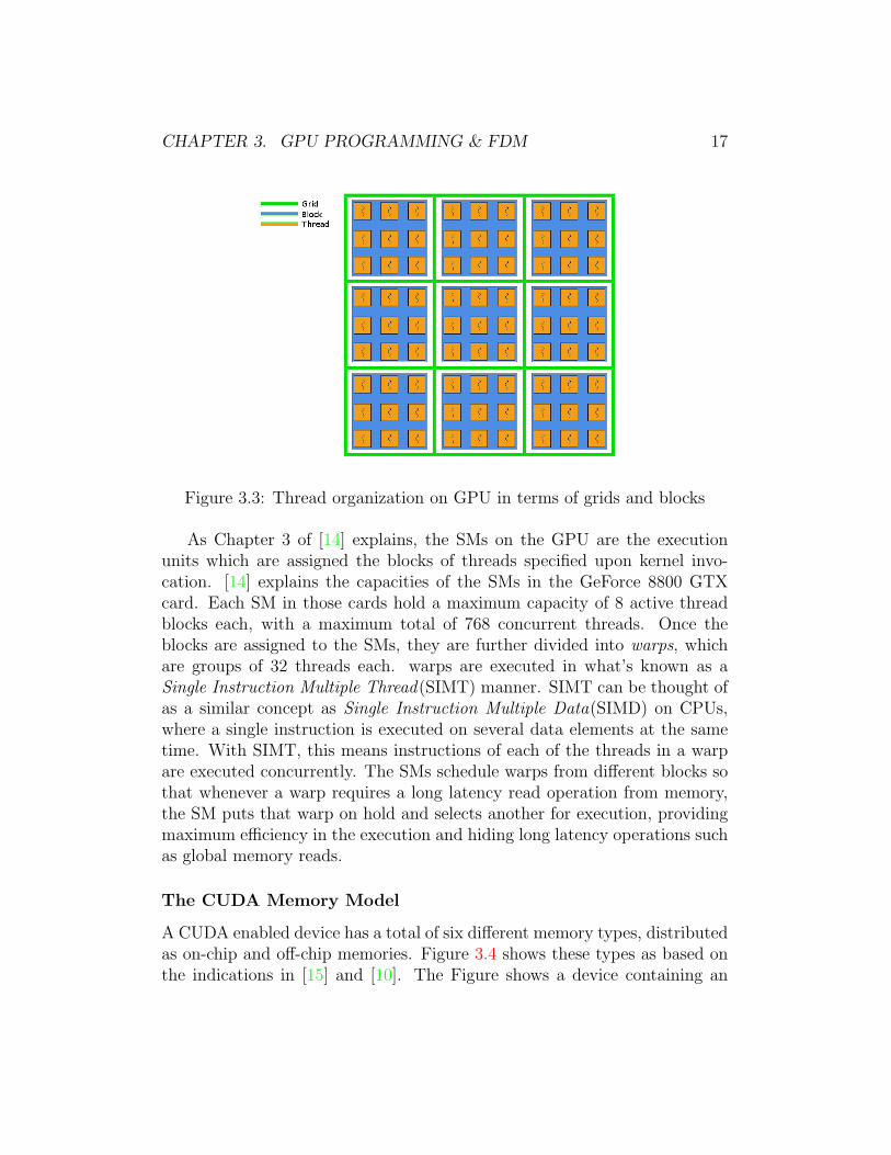
C for CUDA is the programming language used to program CUDA enableddevices. The language is based on the ANSI C programming language, withsome CUDA specific extensions. When developing a CUDA program, thesource code separates code segments which will be run on the host (CPU)and the device (GPU). Device code is written as kernels, which is functionsthat correspond to a single thread run on a streaming multiprocessor(SM)(depicted in Figure 3.2). When such a kernel function is invoked, the pro-grammer specifies how many instances/threads of the kernel will be executedon the GPU in terms of number of blocks of threads. The blocks in this execu-tion configuration are arranged in a two-dimensional grid, where each block isa three-dimensional array of threads. The relationship between grids, blocksand threads is explained in [10] and [14]. Figure 3.3 shows an arrangement ofa grid with dimensionality 3x3, containing blocks of 3x3x1 threads, totaling81 threads.


Figure 3.3: Thread organization on GPU in terms of grids and blocks

As Chapter 3 of [14] explains, the SMs on the GPU are the executionunits which are assigned the blocks of threads specified upon kernel invo-cation. [14] explains the capacities of the SMs in the GeForce 8800 GTXcard. Each SM in those cards hold a maximum capacity of 8 active threadblocks each, with a maximum total of 768 concurrent threads. Once theblocks are assigned to the SMs, they are further divided into warps, whichare groups of 32 threads each. warps are executed in what’s known as aSingle Instruction Multiple Thread(SIMT) manner. SIMT can be thought ofas a similar concept as Single Instruction Multiple Data(SIMD) on CPUs,where a single instruction is executed on several data elements at the sametime. With SIMT, this means instructions of each of the threads in a warpare executed concurrently. The SMs schedule warps from different blocks sothat whenever a warp requires a long latency read operation from memory,the SM puts that warp on hold and selects another for execution, providingmaximum efficiency in the execution and hiding long latency operations suchas global memory reads.

The CUDA Memory Model

A CUDA enabled device has a total of six different memory types, distributedas on-chip and off-chip memories. Figure 3.4 shows these types as based onthe indications in [15] and [10]. The Figure shows a device containing an


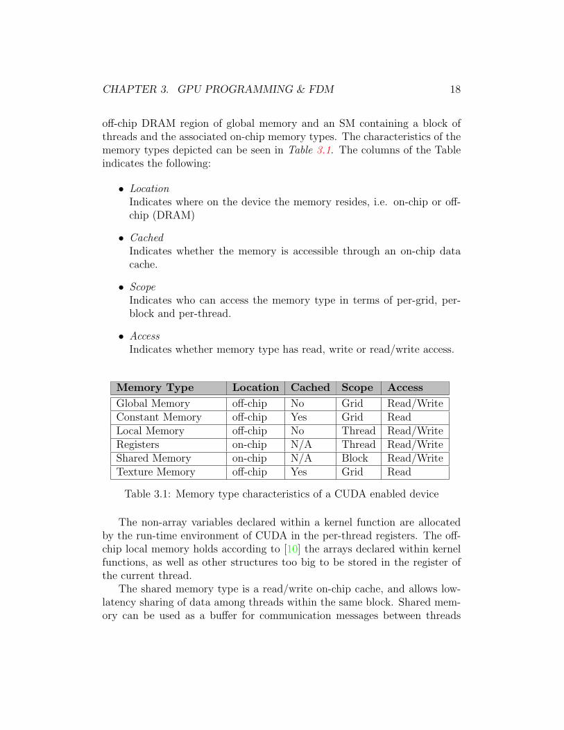
off-chip DRAM region of global memory and an SM containing a block ofthreads and the associated on-chip memory types. The characteristics of thememory types depicted can be seen in Table 3.1. The columns of the Tableindicates the following:

• LocationIndicates where on the device the memory resides, i.e. on-chip or off-chip (DRAM)

• CachedIndicates whether the memory is accessible through an on-chip datacache.

• ScopeIndicates who can access the memory type in terms of per-grid, per-block and per-thread.

• AccessIndicates whether memory type has read, write or read/write access.

Memory Type Location Cached Scope Access

Global Memory off-chip No Grid Read/WriteConstant Memory off-chip Yes Grid ReadLocal Memory off-chip No Thread Read/WriteRegisters on-chip N/A Thread Read/WriteShared Memory on-chip N/A Block Read/WriteTexture Memory off-chip Yes Grid Read

Table 3.1: Memory type characteristics of a CUDA enabled device

The non-array variables declared within a kernel function are allocatedby the run-time environment of CUDA in the per-thread registers. The off-chip local memory holds according to [10] the arrays declared within kernelfunctions, as well as other structures too big to be stored in the register ofthe current thread.

The shared memory type is a read/write on-chip cache, and allows low-latency sharing of data among threads within the same block. Shared mem-ory can be used as a buffer for communication messages between threads


within the same block. The way this works, is that threads write their mes-sages to the shared memory, then synchronizes through a barrier, and finallyreads back the messages from the shared memory.

Figure 3.4: CUDA Memory Layout, Showing the different memory types

Texture memory is a read only portion of the global DRAM, and has anassociated on-chip cache as depicted in Figure 3.4. [10] indicates that thistype of memory is optimized for 2D spatial locality, meaning it is efficient forreading 2D structures. Constant memory is similarly to texture memory, aread-only memory type which has an on-chip cache. Memory access patternshas a great impact on performance. The high degree of control given by theCUDA memory hierarchy makes it easier to optimize this aspect of a GPUapplication.

3.3 The Finite Difference Method (FDM)

Solving Partial Differential Equations (PDEs) requires that we discretize theproblem before implementing a solver. The terms in these equations involvepartial differentials, which we can approximate with numerical differentiation


by means of the Finite Difference Method (FDM) (see e.g. Chapter 8.6 of[16]).

If we want to approximate a first derivative of a function f(x) with respectto x, e.g.

f′(x) =

df(x)

dx(3.1)

we can for use the following approximations

f′(x) ≈ f(x+ ∆x)− f(x)

∆x(3.2)

f′(x) ≈ f(x)− f(x−∆x)

∆x(3.3)

f′(x) ≈ f(x+ ∆x)− f(x−∆x)

2∆x(3.4)

where ∆x is the distance between successive discrete points in the func-tion, 3.2 is the forward difference approximation, 3.3 is the backward dif-ference approximation and 3.4 is the most accurate of the 3; the centereddifference approximation. For the second derivative of a function f(x) withrespect to x, e.g.

f′′(x) =

d2f(x)

dx2(3.5)

we get a centered difference approximation like this (equation 3.6):

f′′(x) ≈ f(x+ ∆x)− 2f(x) + f(x−∆x)

(∆x)2(3.6)

The accuracy of the previously mentioned approximations can be furtherimproved by considering additional off center points, e.g. by adding x ±2∆x, x±3∆x... to the equations and appropriately adjusting the denominatorto account for the new expanded range of the approximation. An exampleof adding an additional point to either side of the first derivative centeredapproximation looks like this:

f′(x) ≈ (f(x+ 2∆x) + f(x+ ∆x))− (f(x− 2∆x) + f(x−∆x))

4∆x(3.7)


For a two dimensional function f(x, z), we can approximate its first order

partial derivative with respect to x, ∂f(x,z)∂x

with e.g. a centered differenceapproximation like the one in Equation 3.7 like this:

∂xf(x, z) ≈ (f(x+ 2∆x, z) + f(x+ ∆x, z))− (f(x− 2∆x, z) + f(x−∆x, z))

4∆x(3.8)

Equation 3.8 can be visualized as a 1 dimensional stencil over the 2 di-mensional solution area, depicted in Figure 3.5

Figure 3.5: Visualization of the centered difference approximation in Equa-tion 3.8. Point computed is in green, while evaluated points are in red

3.4 Related Work on CUDA GPU Offloading

Chapter 38 of [3] presents work done by CGGVeritas on implementing CUDAbased GPU computational offloading for a seismic imaging application. Thealgorithm of the application, referred to as SRMIP, performs seismic mi-gration. Central to this algorithm is acoustic wave propagation, which isperformed by a finite-differencing algorithm in the frequency domain. Per-formance comparisons of the developed GPU offloading implementation inthis work show results of 8-15X speedup with a NVIDIA G80 based GPU(Quadro FX 5600) over an optimized single threaded version of the originalCPU based implementation.

[17] is an article covering a 3D finite differencing computation done withCUDA enabled hardware. The article covers two implementations, one forjust doing computations with a 3D finite differencing stencil, and the other


for computing a finite difference approximated wave equation. The waveequation discretization is also implemented with support for multiple GPUs,where the domain of the computation is partitioned among the differentGPUs, allowing for larger problem sizes. In the multi-GPU version, thedecomposition of the domain distributes e.g. for the 2 GPU case, each of theGPUs gets half the domain + a layer of points overlapping the other half.The multi-GPU implementation of the article shows a throughput for e.g. a4 GPU (Tesla S1070) computing a volume of dimensions 480× 480× 800, of11845.9 million points per second.

[4] is an article which describes the implementation of the Navier-Stokesequations for incompressible fluids. The discretization made of the equationsinvolves centered second order finite difference approximations. The imple-mentation in this article uses double precision calculations on a NVIDIAQuadro FX5800 4GB card, and shows a speedup of 8X compared to a multi-threaded Fortran code running on an 8 core dual socket Intel Xeon E5420CPU. This kind of speedup is especially impressive considering the fact thatthere are only 1 double precision stream processor on each of the 30 streamingmultiprocessors of the GPU.

Chapter 4

Application Analysis andOptimization

In this Chapter, we will begin by profiling our application, identifying theareas in need of GPU computational offloading. Once these areas have beenidentified, we will describe their workings before proceeding with implement-ing GPU replacements for them.

We will go through the different GPU implementations step by step,continually adding new optimizations, explaining motivations for them, aswell as implementation details. We end this Chapter by describing the detailsof adding multiple GPU support to our application.

4.1 Profiling and Analysis

While the core computational areas of this application is known to us be-forehand, profiling the application will allow us to easily identify the sourcecode areas in need of GPU offloading. We will use the Valgrind[18] basedtool CallGrind, which profiles the call paths for an application, as well as theduration for each of the called functions.

The results obtained by running the single processor version of our ap-plication through the CallGrind tool can be seen in Figure 4.1. Here it isseen that the subroutine Fd2dModfd is the main contributor of the com-putational overhead of the application. Looking further down, we see thatthe Fd2dTimestep subroutine is being called 13334 times. For each call tothis subroutine, four different subroutines (DerDifxfw, DerDifyfw, DerDifxba,

23

CHAPTER 4. APPLICATION ANALYSIS AND OPTIMIZATION 24

Figure 4.1: Function call path of our application obtained from the CallGrindtool

DerDifyba) are called.The Fd2dTimestep routine performs a single time step of the finite dif-

ference method applied to the 2D acoustic equations of motion,

ρ ∗ ∂tvx = ∂xσ (4.1)

ρ ∗ ∂tvz = ∂zσ (4.2)

and the constitutive relation,

∂tσ = K ∗ ∂ivi + ∂tI (4.3)

Einstein’s summation convention i is used, where i = (x, z), the ∗ operatordenotes time convolution, and I = I(t, x, z) is the source of injection type.The equations above are performed on a regular 2D grid, and solves for thestress σ components. The equations are relating the particle velocities vx

and vz, the density ρ and the bulk modulus K. x and z in the equationsdenote the horizontal and vertical axis respectively, and t denotes the time.The first order time derivatives in the previous equations (4.1, 4.2, 4.3) areapproximated with backward and forward finite differences,

∂tfn− 12

=fn − fn−1

∆t(4.4)


, and

∂tfn+ 12

=fn+1 − fn

∆t(4.5)

As we can see in the two previous equations, the ∂tf are evaluated half agrid point behind and in front of the current grid point respectively. In thesame 3 PDE equations, the spatial derivatives are approximated using an 8thorder centered difference approximation (see [19]), e.g. in the x direction as,

d−x σ(n, k − 1

2, l) =

1

∆x

8∑m=1

αm[σ(n, k + (m− 1), l)− σ(n, k −m, l)] (4.6)

and

d+x σ(n, k +

1

2, l) =

1

∆x

8∑m=1

αm[σ(n, k +m, l)− σ(n, k − (m− 1), l)] (4.7)

As with the temporal approximations seen in Equations 4.4 and 4.5, wesee that the resulting stress is evaluated half a grid point behind or in frontof the current grid point respectively (seen as k − 1

2and k + 1

2respectively).

This half point spacing shows that our application uses a staggered grid bothin time and in space (see Appendix C in [6]). The difference approximationsin Equations 4.6 and 4.7 are defined with differentiator coefficients αm, whichare pre-computed values. The values of these coefficients are computed bymatching the Fourier spectrum of the approximated differentiators with theFourier spectrum of a perfect differentiator (see [19]).

Equations 4.6 and 4.7 for the x-direction, and similar equations for thez-direction, are located in the DerDixxxx routines we observed in the callgraph of Figure 4.1. In the original application, the order of these differen-tiators is determined by how many points before and after the point beingcomputed are considered, and can be selected in the range [1− 8], where the8th order gives the most accurate result. In our implementations, as shownin Equations 4.6 and 4.7, we will only consider the 8th order differentiators.

Reflections of wave energy from the edges of the modeling domain isabsorbed using the PML absorbing layer detailed in [20], [21] and [22].


Figure 4.2: Problem domain with added PML layers

As there are 4 differentiations being performed for each time step, thePML absorption is done on the borders in the direction of the differentiationfor each of these. The problem domain with the added PML boundary regionscan be seen in Figure 4.2.

Figure 4.3 shows the central work flow of the modeling routine Fd2dModfd.All steps contained within the enclosing blue rectangle in the center of theFigure are part of the Fd2dTimestep routine.

Figure 4.3: Modeling loop of the Fd2dModfd routine

The dimensions of the modeled area are Nx in the horizontal directionand Nz in the vertical direction. The width of the PML layers seen in Figure4.2 is denoted Npml, making the dimensions of the 2 layers in the horizontaldimension [Npml]x[Nz], and the 2 layer in the vertical direction [Nx]x[Npml].


Finally, the order of the finite difference stencil is denoted Nhl. The fourdifferentiator functions in Fd2dTimestep do finite differencing within thetotal modeled domain, including the PML layers (i.e. the total area shown inFigure 4.2). This makes the differentiators span an area of [Nx +Npml]x[Nz +Npml]. The PML layer absorption steps of Fd2dTimestep only computesvalues that span the dimensions of the respective layers.

4.2 Implementing GPU Offloading

The source code of SplFd2dmod is mostly written in the Fortran 90 standard,with some older components written in Fortran 77. Since CUDA is a languageextending ANSI C, as mentioned in Chapter 2, our implementation usesmixed programming, in which we use a Fortran 2003 feature which enableswriting modules with interface declarations pointing to the CUDA sourcefunctions.

Our first approach is moving the computations performed for each timestep to the GPU, i.e. porting the functionality of the Fd2dTimestep routinedepicted in 4.3. The first step in order to achieve this is moving the rele-vant data values for the computations to the GPU. We have made Fortraninterface declarations for CUDAs memory management functions, namelycudaMalloc, cudaMemcpy and cudaFree, which do allocation, copying andde-allocation, respectively. These interfaces are called within the Fd2dModfdroutine, allocating and copying all the relevant values to the GPU device,and once modeling completes, de-allocates the associated memory. Once thenecessary data values are moved to the GPU device, we proceed by imple-menting CUDA kernel functions for each of the Fd2dTimestep steps in Figure4.3.

Common to all of the following implementations, the modeling routine,Fd2dModfd, downloads the relevant stress (σ) values from the device aftereach GPU invocation of the steps in the Fd2dTimestep. The dimension of thedownloaded stress values is equivalent to a single line of the modeled area,i.e. Nx. Another common point is that all kernels have the same executionconfiguration, that is, they are all executed in a grid accommodating the totalsize of the model area ([Nx+Npml]x[Nz +Npml]), with thread blocks of dimen-sions 16x16. Figure 4.4 shows this configuration superimposed on the Figureof the total area (4.2). Finally, the ”Add sources as stress” part of Figure 4.3,is implemented with the same kernel across the different implementations.


The kernel is very small, and only performs a simple vector-matrix addition.

Figure 4.4: Execution configuration superimposed on the total working areaof the model (compare with Figure 4.2)

4.2.1 First Implementation

In this implementation, we partition the steps in Figure 4.3 into 7 separatekernels as shown in Figure 4.5. The order in which these kernels are invokedis the same as in 4.3, i.e. ”Kernel 1 → Kernel 6 → Kernel 2 → Kernel 7→ Kernel 5 → Kernel 3 → Kernel 6 → Kernel 4 → Kernel 7 ”. The kernelinvocation count for one time step of the Fd2dTimestep routine becomes 9for this first implementation.

Figure 4.5: Logical kernel assignment for the first implementation of theFd2dTimestep routine. See Figure 4.3 for reference

The tasks performed by the different kernels in Figure 4.5 can be sum-marized as follows:

• Differentiator Kernels


1. Kernels 1 and 2 are solving for the velocity (v) components in thehorizontal and vertical directions respectively. The equation formof these operations is equivalent to that of Equation 4.7 expandedin both spatial directions, with σ substituted with v.

2. Kernels 3 and 4 are solving for the stress (σ) components in thehorizontal and vertical directions respectively. The equation formof these operations is equivalent to that of Equation 4.6 expandedin both spatial directions.

• PML Kernels

1. Kernel 6 absorbs wave energy reflected off the horizontal bordersresulting from the computations in kernels 1 and 3

2. Kernel 7 absorbs wave energy reflected off the vertical bordersresulting from the computations in kernels 2 and 4

Looking back at the stencil shown in Figure 3.5, the 8th order centereddifferentiators of Kernels 1-4 have a similar shape, with the exception thatthere are a total of 16 contiguous values in either direction being evaluatedfor a point located half a grid point in front or behind the center of thestencil. Keeping in mind that the domain is a staggered grid, this meansthat the computed output point is located in a different, overlapping gridshifted half a grid point off the grid with the evaluated (old) values.

Figure 4.6 shows the 3 different paths threads within the horizontallydifferentiating kernels take. The Figure shows the complete domain of themodel, including PML layers. Considering the stencil of the horizontallydifferentiating kernels (1,3), if a kernel thread is within region 2 of the Figure,all points in the stencil are used in computing the new point. If the thread islocated within regions 1 or 3, some of the evaluated points of the stencil willbe outside the domain. These points are treated as 0 in the computations,effectively shrinking the half of the stencil facing the border of the domain.The vertically differentiating kernels work in the exact same way, only in thez direction.


Figure 4.6: Horizontal differentiator regions of computation

All kernels of this implementation use only the non-cached global memoryof the GPU device see Figure 3.4).

4.2.2 Second Implementation

Now that a working implementation has been achieved, its time to do op-timizations. The related finite differencing done in [17] uses primarily theon-chip per-SM shared memory of the GPU. According to Chapter 5 of [10],reads from shared memory is a lot faster than global memory reads. Ac-cording to [15] and [10], reading memory from the global memory space hasin addition to the 4 clock cycles required to issue the read instruction for awarp, an added latency of about 400-600 clock cycles. Once shared memoryis loaded into its memory space on the SM, [10] states that given no bankconflicts among threads of the same warp, accessing shared memory can beas fast as accessing registers, which generally cost no more than the 4 clockcycles to issue the read instruction.

Using shared memory in this implementation should prove beneficial dueto the fact that several of the memory locations read by threads spaced withinthe half-length of the differentiator stencils read several common values.

We denote the differentiator stencil half length (order), Nhl, and the widthand height of a thread block Nb. We prepare a 2D shared memory area ofsize [2Nhl +Nb]×[Nb] for the horizontal, and [Nb]×[2Nhl +Nb] for the verticaldifferentiator kernels. The threads of a thread block is logically placed at thecenter region of the shared memory area. Each thread reads a single value


from its calculated location in the problem domain into its relative location inthe shared memory region. For the horizontal differentiator kernels, threadswhich are at a distance d <= Nhl from the left border, reads values locatedNhl points to the left, and Nhl + Nb points to the right into correspond-ing locations in shared memory. The same is done in the vertical directionwith threads located Nhl points below the upper border. The loaded sharedmemory regions for blocks of both the horizontal and vertical differentiatorkernels is depicted in Figures 4.7 and 4.8, respectively. Finally, the differen-tiator coefficient values (α) are loaded into a 1D shared memory area by thefirst Nhl threads of the thread block. At the end of all the preceding sharedmemory load operations, all kernels within the same block are synchronized,ensuring that all values are loaded beyond that point.

Figure 4.7: Shared memory region forthread blocks in the horizontal differ-entiators

Figure 4.8: Shared memory region forthread blocks in the vertical differen-tiators

In the first implementation, the number of kernel invocations is 9. Sinceall threads of each of the kernels in that implementation is mapped to thesame problem domain, more of the kernels could be combined, minimizingthe number of invocations per time step. Looking back at the computationalsteps of each time step in Figure 4.3, we note that the PML operations af-ter each differentiation can be combined with the preceding differentiator.The only requirement for doing this is adding conditionals to the differen-tiator kernels. For the horizontal differentiators, these conditionals wouldcheck whether the current thread of the kernel resides within the boundariesof either the left or the right PML layer, and perform the PML operationsaccordingly. An equivalent approach can be made for the vertical differen-tiators. By doing this, we reduce the kernel invocation count by 4, which


makes the new total 5. The five kernels and their scope compared to Figure4.3, can be seen in Figure 4.9.

Figure 4.9: Logical kernel assignment for the second implementation of theFd2dTimestep routine. See Figure 4.3 for reference

The whole modeling routine depicted in 4.3 performs memory transfersfrom the GPU to the host for every time step. We can optimize these transfersby using page locked host memory. What this means is that the page inhost RAM containing the memory target of the transfer, is pinned to a fixedposition, ensuring that the host operating system is unable to move it around.Doing this speeds up memory transfers from the GPU as the transfers areperformed using Direct Memory Access (DMA), circumventing the CPU andthus lowering the transfer latency (see [23])

Summarizing the optimizations made in this second implementation, wehave a total of 5 kernels, 4 of which perform combined differentiation andPML absorption. The differentiators uses shared memory for the stencilvalues, as well as the differentiator coefficients (σ). The PML calculations stillonly perform global memory read/writes. Finally, page allocated memory forthe per time step GPU → host transfers has been employed.

4.2.3 Third Implementation

In this implementation, we further reduce the kernel invocation count bycombining more of the steps in 4.3. All of the operations to the left of addsources are combined, and similarly, all operations at the right are combined.The total number of kernels now becomes 3, which can be seen in Figure 4.10.Both of these differentiator/PML kernels are now performing operations inboth directions of the domain, doing the equivalent of Equation 4.7 for thekernel on the left (Kernel 1), and 4.6 for the kernel on the right (Kernel 3).


Figure 4.10: Logical kernel assignment for the third implementation of theFd2dTimestep routine. See Figure 4.3 for reference

While the previous implementation used shared memory regions of Nb ×(Nb + 2Nhl) elements each. For the combined kernels of this implementation,the shared memory regions would have to be further expanded to dimension(Nb+2Nhl)×(Nb+2Nhl) in order to accommodate all necessary values of bothdirections. Another problem here is that the left kernel solves for the velocity(vx) components in horizontal direction, followed by the separate velocity (vz)components in the vertical direction. This would complicate shared memoryusage by either needing to prepare two separate shared memory regions foreach of the velocity fields, or by re-loading new values into shared memorybetween differentiations. Both cases would also further complicate threadindexing, and also requiring added registers and control flow.

Reverting back to global memory is not really an option in this implemen-tation, since we know that reads from the global memory space is expensive,and that threads within a block tends to read several common values, some-thing that would benefit from some kind of data caching. Looking at thearchitectural layout in 3.2, we see that the L1 texture cache looks promisingfor use with the differentiators. The texture memory, according to Chapter5 of [10], is considerably faster than global memory reads, since it only needsto access the global memory on cache misses, i.e. when a thread tries to geta value not currently in the cache. It is also indicated that texture memoryreads have less constraints on the memory access pattern compared to globaland constant memory.

We implement texture memory with the two differentiator/PML kernelsof this implementation. The way we do this, is to create 3 1D texture (forσ, vx and vz ) with dimensions equal to the total area of the problem domain,i.e. (2Npml + Nx) × (2Npml + Nz). 1D textures is a natural choice for thisimplementation due to the fact that the memory areas of e.g. σ and vx, vz islocated in linear memory where logical 2D addressing in the problem domainis stated as e.g. σ[x][z] = σ[z × (2Npml +Nz) + x]. Reads from the texturesare performed through the CUDA API function, which for e.g. fetches in σ


looks like: ”σ[index] = tex1Dfetch( texture σ, index )”.Summarizing the changes made in this implementation, we have joined

Kernels 1-2 and Kernels 4-5 of the previous implementation (see Figure 4.9,and used texture memory for the evaluated values of the differentiator sten-cils. The differentiator coefficients remain, as in the previous implementation,in shared memory, since there are only 2 1D arrays of coefficients for each ofthe two kernels, each with dimension Nhl (i.e. 8).

4.3 Multi GPU

SplFd2dmod is, as mentioned in Chapter 2, MPI enabled. Since the frame-work for parallelism is already implemented in this manner, we have added afeature which enables the slave processes spawned in MPI mode to use GPUcomputational offloading if there is an available GPU for this process. Theway this works is by passing an argument to the application, gpn, indicatinghow many GPU devices are available per node/workstation. The first gpnprocesses of each node runs the GPU version, while the remaining processesfor that node runs regular CPU computations. By allowing a hybrid solutionlike this, resource utilization is effectively maximized. The updated flow di-agram for the application can be seen in Figure 4.11. A requirement for thisfeature is that each node the application uses have the same fixed numberof GPU compute devices. We have implemented this feature for all the 3different GPU enabled implementations.


Figure 4.11: Updated work flow for hybrid CPU/GPU implementation

Chapter 5

Results & Discussion

In this Chapter we will compare the performance of our original applicationand the various optimized GPU versions discussed in the previous Chapter.The comparisons will be run on two different workstations, and we will endthis Chapter with a discussion of the results obtained.

5.1 Methodology

For our benchmarking, time will be the metric used. Also, relative speedupwith respect to the original application will be measured for each of the GPUversions mentioned in the previous Chapter. The speedup is calculated asfollows:

S =torig

tgpu

(5.1)

Where S is the speedup factor, torig is the run time of the original appli-cation, and tgpu is the run time of the application with GPU offloading.

For each benchmark, we present a performance graph based on the aver-age run time for a specific configuration over the course of 4 samples/runs.This average is calculated with the following equation:

taverage =1

n

n∑i=1

ti (5.2)

The timings done in the tests are performed for the core computationalkernel of the the Fd2dModfd routine, so data preparations are not included

36

CHAPTER 5. RESULTS & DISCUSSION 37

in the measurements despite the fact that they only incur an additional runtime of a few seconds.

5.2 Test Systems

Our benchmarks will be obtained from two of the workstations availableat the High Performance Computing Lab (HPC-Lab) run by Dr. Elster atthe Department of Computer and Information Science (IDI). The hardwarecharacteristics of these workstations are listed in Table 5.1.

System CPU RAM Storage GPUHPC lab 1 Intel Core2 Quad

Q9550 @2.83GHz4GB 41GB NVIDIA GeForce GTX280

NVIDIA Tesla C1060HPC lab 2 Intel Core I7 965

@3.20GHz12GB 1.4TB NVIDIA Tesla S1070

(4X NVIDIA Tesla C1060)

Table 5.1: Hardware Characteristics

The operating system used for the two workstations in Table 5.1, is a64 bit (x86 64) Ubuntu 9.04 distribution running a v2.6.28-11 Linux kernel.HPC lab 1 uses a v2.1 release of the CUDA software development toolkit,while HPC lab 2 uses a v2.2 release. The original version of SplFd2dmod hasbeen compiled on both workstations using the Intel Fortran Compiler v10.1.For the GPU utilizing implementations, the NVCC compiler of the CUDAsoftware development toolkit has been used. CUDA host code is compiled byNVCC using the systems’ GCC compiler. For HPC lab 1, the GCC versionis 4.2.4, while HPC lab 2 uses version 4.3.3.

Common to all GPUs listed in Table above, is that they are connectedwith the PCI Express 2.0 interface. The S1070 in HPC lab 2 is connectedwith 2 such interfaces.

5.3 Benchmark Results

5.3.1 Results from the HPC workstations

These results are obtained from the HPC lab workstations mentioned in Ta-ble 5.1. Each of these tests show results from modeling a single shot withthe original, unmodified CPU based version in single processor mode, and


the 3 GPU enabled versions. The total dimensions, including 20 points widePML layers on all sides, is 1481x1101, requiring a total of 6072 thread blocksof dimension 16× 16 for each kernel invocation of the different GPU imple-mentations. The total thread count for each of these invocations becomes6072×16×16 = 1554432. The following 3 tests benchmark the performanceof modeling a shot with these dimensions, doing a total of 13334 invocationsof the Fd2dTimestep computations depicted in Figure 4.3.

The results shown in Figures 5.1 and 5.2 show the performance of themodeling on the HPC lab 1 workstation mentioned in Table 5.1 for the singleprocessor mode of the original application, as well as single processor modeversions of the 3 different GPU implementations detailed in the previousChapter. These two Figures show the performance of using the NVIDIAGeForce GTX280 and NVIDIA Tesla C1060 GPU, respectively. Figure 5.3,shows the same tests for the HPC lab 2 workstation, using one of the 4NVIDIA Tesla C1060 GPUs of the NVIDIA Tesla S1070 rack unit. All 3of the following test results show average timings in seconds for 4 runs (seeequation 5.2). The Figures also show speedup (see equation 5.1) relative tothe original CPU version.

Figure 5.1: HPC lab 1 running NVIDIA GeForce GTX280


Figure 5.2: HPC lab 1 running NVIDIA Tesla C1060

Figure 5.3: HPC lab 2 running single NVIDIA Tesla C1060


5.3.2 Scaling Characteristics

Here we show how well the CPU and GPU versions scale when adding moreCPUs/GPUs to the computation on the workstations. Results are collectedfrom the HPC lab 2 workstation listed in Table 5.1. While tests could havebeen run on HPC lab 1 as well, its GPU configuration is heterogeneous,which will make the results less predictable.

Both tests will run 4 times, adding 1 processing unit to the computa-tion each time. The application will run with the I/O server as a separateprocess, distributing 12 shots for every run among the participating slaveprocessing units. Running the application in this way will make the totalrange of processes running for each configuration [2 − 5]. The main reasonfor modeling 12 shots, is that this amount of work increases the chances of aneven workload distribution among the participating slave processing units.

Figure 5.4: CPU Scaling results with {1,2,3,4} processes


Figure 5.5: GPU Scaling results with {1,2,3,4} processes

5.4 Discussion

The results from the HPC lab 1 workstation shown in Figures 5.1 and 5.2,show a fairly significant performance decrease for the first GPU implemen-tation (GPUv1 ) running on the Tesla C1060. The reason for this can beattributed to the memory bandwidth difference between the GTX280 andthe C1060. For the C1060, memory bandwidth is 102GB/s (see [24]), whilethe GTX280 has a bandwidth of 141.7GB/s (see [25]) which amounts to adifference of approximately 28%. This performance difference can also beseen for the other 2 GPU implementations, but with less impact. The rea-son for this is that GPUv2, which uses shared memory, does far less readsfrom global memory compared to GPUv1. The relatively large performancedifferences between the three implementations are mainly attributed to thefact that the algorithms perform very few operations for each element readfrom memory; i.e. they are what is known as memory bound.

The performance jump between GPUv2 and GPUv3 is largely due tothe use of texture memory, and implies that even fewer memory reads areperformed due to the higher cache utilization of this final implementation.


The merging of Kernels performed for this implementation also means thatsome of the kernel invocation overhead from GPUv2 is removed. GPUv2requires additional address computations for the shared memory reads, aswell as some extra conditional branches. Both of these requirements havebeen removed in GPUv3, which has also had an impact on performance.

The performance results shown in Figure 5.3 are as expected, the samefor the GPU versions as the results of Figure 5.2, this due to the factthat the C1060 is the GPU device running the tests for both workstations(S1070=4×C1060).

For the scaling tests, we observe that near linear scaling is achieved withthe S1070, but not with the CPUs. This is not surprising, since the appli-cation parallelizes the work by assigning different shots to the different slaveprocesses. Since the processes running on the CPU share the same cache andsystem memory, per-process performance will decrease as more processes areadded. As an added note, we confirmed that our strategy for ensuring evenworkload distribution worked by looking at the application output for theparticipating processes. All slave processes modeled the same number ofshots for each of the tests in both the CPU and GPU case.

The linear scaling of the GPUs can be attributed to the fact that noneof them have to share any of the memory or computing resources with otherprocesses. The tiny portion of interaction with the CPU and the host memoryis too small to make an impact from the 1 GPU to the 4 GPU case.

Finally, as we have looked at the compiler output of all of the implemen-tations, we see that the memory requirements (registers and shared memory)per kernel are sufficiently low to allow full SM occupancy. What this means isthat each SM of the GPU is able to run 4 blocks, or 1024 threads (maximumof capacity for Compute Capability 1.3, see Appendix A of [10]), simultane-ously. The effect of being able to accommodate this amount of threads, isthat when a warp executed by the SM issues a long latency read operation,the thread scheduler switches to another warp while the memory operationis performed, effectively hiding memory latency.

Chapter 6

Conclusions & Future Work

In this thesis we analyzed a seismic application for shot processing and suc-cessfully developed and implemented a GPU-accelerated version. Our resultsachieved considerable speedups compared to the original implementation.Implementing the GPU off-loading was done with only minimal modificationsto the original source code, primarily in the core modeling function. SinceFortran continues to often be the programming language of choice in thegeophysical applications at StatoilHydro, this ability to keep the large por-tions of source code unchanged when implementing GPU off-loading, greatlyreduced the programming efforts required.

An understanding of parallel programming and the C/C++ programminglanguage are the most fundamental requirements for developing CUDA appli-cations. From our experiences developing the GPU implementations of thisthesis, the biggest challenge, not being familiar with CUDA programmingbeforehand, was getting a clear understanding of the targeted application.Learning to use the CUDA programming API was not that time consuming,since it is generally well structured and documented. The efforts put intolearning CUDA programming was hence for us certainly a lot smaller thanthose required for understanding the geophysical aspects of the application.Based on these experiences, we gather that the development efforts requiredfor the developers at StatoilHydro should also be reasonably small.

As was mentioned in the previous paragraph, understanding the targetedapplication was quite the challenge for this Computer Science student. Be-cause of this, the first working GPU off-loading implementation was readyonly 6 weeks prior of submitting this thesis. This fact should be a clear indi-cation of the potential for positive results in the course of a relatively small

43

CHAPTER 6. CONCLUSIONS & FUTURE WORK 44

developing period.Applications with computational kernels performing data parallel compu-

tations are a good match for the data parallel nature of GPU devices. Thecomputational kernel of our application proved to be fairly data parallel innature, with few serial dependencies. This fact made it a good match forGPU off-loading.

Our benchmarks were done on two different systems in the NTNU IDI(Department of Computer and Information Science) HPC-lab. One systemwas a Intel Core2 Quad Q9550 @2.83GHz with 4GB of RAM and an NVIDIAGeForce GTX280 and NVIDIA Tesla C1060 GPU. Our second testbed wasan Intel Core I7 Extreme (965 @3.20GHz) with 12GB of RAM hosting anNVIDIA Tesla S1070 (4X NVIDIA Tesla C1060). On this hardware, speedupsup to a factor of 8-14.79 compared to the original sequential code wereachieved, confirming the potential of GPU computing in applications sim-ilar to the one used in this thesis. The work done in e.g. [17], [4] and [3],also further supports our conclusion.

6.1 Future Work

Since a lot of the time spent completing this work went into understandingthe workings of the targeted application, quite a lot remains to be explored.Following are some of the main issues to be explored further.

6.1.1 GPU Utilizing Mathematical Libraries

We would like to see the potential payoffs associated with using librariessuch as the CUDA based CUFFT for computing Fast Fourier Transform of1, 2 and 3 dimensional data, and the CUBLAS library (an adaptation of theBasic Linear Algebra Subprograms (BLAS)) for linear algebra operations inseismic processing related applications.

6.1.2 Further Improvements to SplFd2dmod

As we discussed in the previous Chapter, the computational kernel does fewarithmetic operations per memory read, i.e. is considered memory bound. Inorder to achieve optimal speedups in such applications, additional attentionto the memory access patterns of the GPU threads is required. We believe


that there’s still potential for higher performance if the memory access pat-terns of our kernels is further analyzed.

Another potential performance optimization could be to eliminate thememory transfers between time steps by keeping these values in GPU mem-ory, only doing transfers to/from the GPU at the beginning and end of themodeling loop. We suspect that the performance benefits from this might berelatively small compared to better memory bandwidth utilization as men-tioned earlier, but it is still a point of interest. Doing this would also requireadditional storage in GPU memory, which depending on problem size, mayor may not prove to be an issue.

Also, the algorithm for the differentiation depicted in Figure 4.6 couldpotentially be improved by treating the entire problem domain as a singleregion. The texture fetch operations of our last implementation (GPUv3 ),has the property of returning a 0 value for fetches made on memory areasnot covered by the texture. This could potentially make it possible for us touse the full width of the differentiator stencil in all regions of the problemdomain, eliminating the need for adjusting the stencil length in the borderingregions, i.e. regions 1 and 3 in Figure 4.6. Treating the entire problem domainas a whole for the differentiators like this, would eliminate the conditionalbranches for selecting regions, making all threads of a block perform thesame operations regardless of relative location in the problem domain, whichshould result in increased performance.

6.1.3 Further Testing

The tests performed in this thesis all model shots based on values of the samedimensions, requiring approximately 116 MB. By increasing the resolutionof the input velocity and density models of the application, we could get abetter view of the applications scaling characteristics with respect to problemsize. The procedure to perform such a re-grid operation was presented to ustoo late to be included in this thesis. It would be of great interest to see theapplications performance characteristics given larger problem sizes.

The multi-GPU functionality of the application has in this thesis onlybeen tested on a single workstation. The reason for this is that we haven’thad access to a compute cluster containing nodes with a distributed filesystem and CUDA enabled GPUs. Performance comparisons of the multi-GPU enabled implementation on such a cluster with the original runningon e.g. one of StatoilHydro’s production clusters would be interesting, and a


likely added incentive for doing further research on GPU based computationaloffloading.

Bibliography

[1] J. D. Owens, M. Houston, D. Luebke, S. Green, J. E. Stone, and J. C.Phillps, “GPU Computing,” Proceedings of the IEEE, vol. 96, May 2008.

[2] D. Blythe, “Rise of the Graphics Processor,” Proceedings of the IEEE,vol. 96, May 2008.

[3] H. Nguyen, C. Zeller, E. Hart, I. Castao, K. Bjorke, K. Myers, andN. Goodnight, GPU Gems 3. Addison-Wesley Professional, August2007.

[4] J. M. Cohen and M. J. Molemaker, “A Fast Double Precision CFD Codeusing CUDA,” 2009.

[5] O. Johansen, “Checkpoint/Restart for Large Parallel Seismic Process-ing Applications,” Master’s thesis, Norwegian University of Science andTechnology (NTNU), January 2009.

[6] L. T. Ikelle and L. Amundsen, Introduction to Petroleum Seismology.No. 12 in Investigations in Geophysics, Society of Exploration Geophysi-cists, 2005.

[7] J. A. Haugen and B. Arntsen, “Spl fd2d module documentation.” For-tran source code documentation. StatoilHydro internal document.

[8] K. Fatahalian and M. Houston, “GPUs - a closer look,” ACM QUEUE,March/April 2008.

[9] “Glsl.” Wikipedia article. Website available at ”http://en.wikipedia.org/wiki/GLSL”, last visited: June 26, 2009.

[10] NVIDIA, Cuda Programming Guide 2.1, December 2008.

47

http://en.wikipedia.org/wiki/GLSL

http://en.wikipedia.org/wiki/GLSL

BIBLIOGRAPHY 48

[11] The Khronos Group, “OpenCL Overview,” February 2009. Websiteavailable at ”http://www.khronos.org/opencl/”, last visited June 26,2009.

[12] A. L. Shimpi and D. Wilson, “NVIDIA’s 1.4 Billion Transistor GPU:GT200 Arrives as the GTX 280 & 260,” AnandTech Web-site, June 2008.Website available at ”http://www.anandtech.com/video/showdoc.aspx?i=3334&p=1”, last visited: June 26, 2009.

[13] NVIDIA, NVIDIA GeForce GTX 200 GPU Architectural Overview, May2008.

[14] D. Kirk and W. Hwu, Cuda textbook. 2008-2009.

[15] R. Farber, “Cuda, Supercomputing for the Masses,” Dr. Dobb’s Por-tal, 2008-2009. Website available at ”http://www.ddj.com/cpp/207200659”, last visited: June 26, 2009.

[16] M. T. Heath, Scientific Computing - An Introductory Survey. McGraw-Hill, second ed., 2002.

[17] P. Micikevicius, “3D Finite Difference Computation on GPUs usingCUDA,” 2009.

[18] “Valgrind Instrumentation Framework.” Website available at ”http://valgrind.org”, last visited: June 26, 2009.

[19] O. Holberg, “Computational Aspects of the choice of Operator and Sam-pling Interval for Numeric Differentiation in Large-scale Simulation ofWave Phenomena,” Geophysical Prospecting, vol. 35, 1987.

[20] J.-P. Berenger, “A Perfectly Matched Layer for the Absorption of Elec-tromagnetic Waves,” Journal of Computational Physics, vol. 114, 1994.

[21] Q.-H. Lui and J. Tao, “The perfectly matched layer for acoustic waves inabsorptive media,” Journal of the Acoustic Society of America, vol. 102,October 1997.

[22] T. Wang and X. Tang, “A Nonsplitting PML for the FDTD Simulationof Acoustic Wave Propagation,” September 2001. Society of ExplorationGeophysicists International Exposition and Annual Meeting.

http://www.khronos.org/opencl/

http://www.anandtech.com/video/showdoc.aspx?i=3334&p=1

http://www.anandtech.com/video/showdoc.aspx?i=3334&p=1

http://www.ddj.com/cpp/207200659

http://www.ddj.com/cpp/207200659

http://valgrind.org

http://valgrind.org

BIBLIOGRAPHY 49

[23] NVIDIA, Cuda Reference Manual 2.1, November 2008.

[24] “Tesla C1060 Board Specification,” September 2008. Websiteavailable at ”http://www.nvidia.com/docs/IO/56483/Tesla_C1060_boardSpec_v03.pdf”, last visited: June 26, 2009.

[25] “NVIDIA GeForce GTX280 Specifications.” Website availableat ”http://www.nvidia.com/object/product_geforce_gtx_280_us.html”, last visited: June 26, 2009.

http://www.nvidia.com/docs/IO/56483/Tesla_C1060_boardSpec_v03.pdf

http://www.nvidia.com/docs/IO/56483/Tesla_C1060_boardSpec_v03.pdf

http://www.nvidia.com/object/product_geforce_gtx_280_us.html

http://www.nvidia.com/object/product_geforce_gtx_280_us.html

Seismic Shot Processing on GPU - NTNU · 2009-08-25 · Seismic processing applications typically...

Documents

Transcript of Seismic Shot Processing on GPU - NTNU · 2009-08-25 · Seismic processing applications typically...