Seismic sensing: Comparison of geophones and ...

Important Notice

This copy may be used only for the purposes of research and

private study, and any use of the copy for a purpose other than research or private study may require the authorization of the copyright owner of the work in

question. Responsibility regarding questions of copyright that may arise in the use of this copy is

assumed by the recipient.

UNIVERSITY OF CALGARY

Seismic sensing: Comparison of geophones and accelerometers using laboratory and field

data

by

Michael S. Hons

A THESIS

SUBMITTED TO THE FACULTY OF GRADUATE STUDIES

IN PARTIAL FULFILMENT OF THE REQUIREMENTS FOR THE

DEGREE OF MASTER OF SCIENCE

DEPARTMENT OF GEOSCIENCE

CALGARY, ALBERTA

JULY, 2008

© Michael S. Hons 2008

ii

UNIVERSITY OF CALGARY

FACULTY OF GRADUATE STUDIES

The undersigned certify that they have read, and recommend to the Faculty of Graduate

Studies for acceptance, a thesis entitled “Seismic sensing: Comparing geophones and

accelerometers using laboratory and field data” submitted by Michael S. Hons in partial

fulfillment of the requirements for the degree of Master of Science.

________________________________________________

Supervisor, Dr. Robert R. Stewart, Department of

Geoscience

________________________________________________

Dr. Don C. Lawton, Department of Geoscience

________________________________________________

Dr. Nigel G. Shrive, Department of Civil Engineering

______________________

Date

iii

ABSTRACT

Accelerometers, based on micro-electromechanical systems (MEMS), and

geophones are compared in theory, laboratory testing and field data. Both sensors may be

considered simple harmonic oscillators. Geophone output is filtered ground velocity and

represents its own domain. Modeling shows that geophone and digital accelerometer

output is similar in appearance. In laboratory tests, both sensors matched their modeled

responses over a wide range of amplitudes. Since the response is accurate in practice, it

is used to calculate ground acceleration from geophone output. Comparison of

acceleration field data at Violet Grove and Spring Coulee shows most reflection energy is

effectively identical from 5 Hz to over 150 Hz. Some consistent differences were noted

under strong motion and in the noise floors. In general, when sensor coupling is

equivalent, the data quality is equivalent.

iv

ACKNOWLEDGEMENTS

I would never have stumbled into the world of seismic sensors and recording instruments

if not for the suggestion by my supervisor, Rob Stewart. This work was helped along at

all stages and in all ways by discussions and input from Glenn Hauer of ARAM Systems

Ltd. His detailed knowledge of industrial quality systems has been a wealth I’ve been

delighted to draw on. Kevin Hall helped provide access to the field data, and prevented

panic at computing malfunctions (“hmm, I hope Kevin can fix that”), while discussions

with Malcolm Bertram about how the things actually work were very helpful. Thanks to

Dr. Swavik Spiewak for bringing me onboard the VASTA project and giving me an

inside look at the lab data collection. The PennWest CO2 monitoring project at Violet

Grove was supported by Alberta Energy Research Institute, Western Economic

Diversification, Natural Resources Canada, and the National Science and Engineering

Research Council of Canada. Finally thanks to my family for support of an emotional

nature, and to the CREWES sponsors for support of a financial nature.

v

To my wife, whose works of beauty and genius that I can only strive to match.

vi

TABLE OF CONTENTS

Approval Page…………………………………………………………………. ii

Abstract………………………………………………………………………... iii

Acknowledgements……………………………………………………………. iv

Dedication……………………………………………………………………... v

Table of Contents……………………………………………………………… vi

List of Tables…………………………………………………………………... viii

List of Figures………………………………………………………………….. ix

CHAPTER ONE: INTRODUCTION AND THEORY ………………………. 1

Overview of thesis…………………………………………………………….. 1

Geophones..…………………………...……………………………………….. 3

Delta-Sigma converters……….………………………. ……………… 11

MEMS accelerometers….………………………………………..……………. 14

Transfer function between accelerometers and geophones…….……………… 22

CHAPTER TWO: MODELING AND LAB RESULTS……….……………… 27

Modeling……………………………………………………………………….. 27

Zero phase wavelets……………………………………………………. 27

Minimum phase wavelets………………………….…………………... 29

Vibroseis/Klauder wavelets……………………………………………. 31

Spiking deconvolution.………………………………………………... 35

Lab results……………………………………………………………………… 42

Vertical orientation..…………………...……………………………….. 45

Medium vibrations………….…………………………………... 46

Ultra weak vibrations.………………………………………….. 48

Horizontal orientation………………………………………………….. 50

Strong vibrations……………………………………………….. 50

Weak vibrations………………………………………….…….. 52

CHAPTER THREE: VIOLET GROVE FIELD DATA……………………….. 54

Experimental design..…………………………………………………............... 54

Recording instruments..………………………………………………………… 57

Antialias filters………………………………………………………….. 57

Preamp gain and scaling………………………………………………… 60

Noise floors…………………………………………………………….. 65

Vertical component data...……………………………………………………… 67

Amplitude spectra (global)……………………………………………… 68

Amplitude spectra (local)……………………………………………….. 76

Phase spectra……………………………………………………………. 81

Time domain filter panels………………………………………………. 84

Crosscorrelation..……………………………………………………….. 89

Horizontal component data…………………………………………………….. 92

Amplitude spectra (global)……………………………………………… 94

Amplitude spectra (local)………………………………………………. 99

vii

Phase spectra……………………………………………………………. 100


Crosscorrelation..……………………………………………………….. 105

Discussion………………………………………………………………………. 108

CHAPTER FOUR: SPRING COULEE FIELD DATA………………………... 110

Experimental design…………………………………………………………….. 110

Recording instruments………………………………………………………….. 110

Scaling………………………………………………………………….. 111

Noise floors…………………………………………………………….. 112

Vertical component……………………………………………………............... 112

Amplitude spectra (global)……………………………………............... 114

Amplitude spectra (local)………………………………………………. 115

Phase spectra…………………………………………………………… 119

Time domain filter panels……………………………………………… 122

Crosscorrelation………………………………………………………… 124

Horizontal component…………………………………………………............... 126

Amplitude spectra (global)……………………………………............... 127

Amplitude spectra (local)……………………………………………….. 128

Phase spectra……………………………………………………………. 132


Crosscorrelation…………………………………………………………. 137

Discussion………………………………………………………………………. 139

CONCLUSIONS……………………………..…………………………………. 140

Future work……………………………………………………………………… 145

REFERENCES……………………………….………………………………… 147

APPENDIX A: Derivation of Simple Harmonic Oscillator equation………..... 149

APPENDIX B: Matlab code for geophone to accelerometer transfer…………. 151

APPENDIX C: Optimal damping for accelerometers…………………………. 155

viii

LIST OF TABLES

1.1 Example of a Delta-Sigma loop in operation…………………………... 13

1.2 Equivalent Input Noise of digitizing units and MEMS accelerometers at a 2 ms

sample rate……………………………………………………………... 26

2.1 Comparison of quoted and tested sensor parameters…………………... 45

2.2 Quoted error bounds of tested sensors…………………………………. 45

3.1 Parameters of sensors and cases at Violet Grove……………………… 55

ix

LIST OF FIGURES

1.1 Geophone element and cutaway cartoon (after ION Geophysical) (suspended

magnet inner, coils outer)……………………………………………… 2

1.2 MEMS accelerometer chip (Colibrys) and cutaway cartoon (Kraft,

1997)…………………………………………………………………… 2

1.3 A simple representation of a moving-coil geophone (modified from ION product

brochure)……………………………………………………………….. 3

1.4 Amplitude and phase spectra of the geophone displacement transfer function.

Resonant frequency is 10 Hz and damping ratio is 0.7………………… 7

1.5 Amplitude and phase spectra of the geophone velocity transfer function.


1.6 Amplitude and phase spectra of the geophone acceleration transfer function.


1.7 Diagram of a Delta-Sigma analog-to-digital converter (Cooper, 2002).. 13

1.8 Noise shaping of Delta Sigma ADCs (Cooper, 2002). The shaded blue box on the

left represents the desired frequency band, with the large green spike representing

signal frequencies. Frequencies greater than the frequency band contain

significantly more noise, but will be filtered prior to recording. ……... 14

1.9 Schematic of a MEMS accelerometer. C1 and C2 are capacitors formed by the

electrode plates. The proof mass is cut out of the central wafer………. 15

1.10 Amplitude and phase spectra of a capacitive sensor relative to ground

displacement. Resonant frequency is 10 Hz and damping ratio is 0.2. Response

has the same shape as a geophone relative to velocity………………… 16

1.11 Amplitude and phase spectra of a capacitive sensor relative to ground velocity.

Resonant frequency is 10 Hz and damping ratio is 0.2. Response has the same

general shape as a geophone relative to acceleration………………….. 17

1.12 Amplitude and phase spectra of a capacitive sensor relative to ground

acceleration. Resonant frequency is 10 Hz and damping ratio is 0.2. Amplitude

from 1 Hz to ~2 Hz is flat (10-20% of ω0)…………………………… 17

1.13 Amplitude and phase spectra for a 1000 Hz, 0.2 damping ratio MEMS

accelerometer with respect to ground acceleration…………………… 19

1.14 Inverse of equation (1.37), representing amplitude changes and phase lags to

calculate ground acceleration from geophone data, once all constant gains have

been taken into account……………………………………………….. 24

1.15 Input ground motion amplitudes as recorded by 10 Hz, 0.7 damping ratio

geophone……………………………………………………………… 25

1.16 Acceleration amplitudes restored……………………………………... 26

1.17 Noise floors of a typical geophone and a typical MEMS accelerometer, shown as

ng……………………………………………………………………… 26

2.1 Ricker displacement wavelet (blue circles) at 25 Hz, velocity wavelet (green

squares), and acceleration wavelet (red triangles)……………………. 27

2.2 For a single ground motion, as long as each domain of ground motion is input to

its appropriate transfer function, the output from a geophone is always the

same…………………………………………………………………… 28

x

2.3 For a single ground motion, as long as each domain of ground motion is input to

its appropriate transfer function, the output from an accelerometer is always the

same……………………………………………………………………... 28

2.4 Raw output from a geophone (blue circles) and MEMS (red triangles) for an input

25 Hz Ricker ground displacement……………………………………… 29

2.5 Minimum phase (25 Hz dominant) ground displacement wavelet (blue circles),

time-derivative ground velocity wavelet (green squares), and double time-

derivative ground acceleration wavelet (red triangles)…………………. 30

2.6 Raw output from a geophone (blue circles) and MEMS (red triangles) for an input

25 Hz impulsive ground displacement………………………………….. 31

2.7 Spectra of an 8-120 Hz linear sweep…………………………………… 33

2.8 Autocorrelation of the 8-120 Hz sweep in Figure 2.7…………………… 33

2.9 Result of convolving Figure 1.26 with a 10 Hz, 0.7 damping geophone ground

displacement transfer function. Also the result of convolving Figure 1.25 with the

transfer function first and correlating with the input sweep second……. 34

2.10 Sweep recorded through accelerometer, then correlated with input sweep. The

result matches with the double time derivative of the Klauder wavelet… 35

2.11 Reflectivity series used for synthetic modeling…………………………. 36

2.12 Amplitude spectrum of reflectivity series. Distribution is not strictly ‘white’, but

it is not overly dominated by either end of the spectrum………………. 36

2.13 Wavelets used in modeling. Implosive source displacement (25 Hz): blue circles.

Ground velocity: green squares. Ground acceleration: red triangles. Raw

geophone output: purple stars…………………………………………… 37

2.14 Amplitude spectra of wavelets in Figure 2.13…………………………… 38

2.15 Ground displacement (green) and velocity (red) for a 25 Hz minimum phase

impulsive displacement wavelet, with reflectivity series (blue)………… 38

2.16 Geophone output trace (purple) and ground acceleration (orange), for a 25 Hz

minimum phase impulsive displacement wavelet, with reflectivity

(blue)…..……………………………………………………………….. 39

2.17 Spiking deconvolution results for ground displacement (green) and velocity (red),

with the true reflectivity (blue)………………….……………………… 40

2.18 Spiking deconvolution results for the geophone trace (purple) and the ground

acceleration trace (orange), with true reflectivity (blue). The results are similar to

each other, but generally poorer than those in Figure 2.17………….….. 40

2.19 Deconvolution results for different random noise amplitudes, added to the ground

displacement…………………………………………………………….. 41

2.20 Deconvolution results for different random noise amplitudes, added to the

recorded trace………………………………………………………….. 42

2.21 Noise spectra recorded during a quiet weekend period (Sunday, 9am).. 44

2.22 Harmonic scan results for geophone GS-42…………………………… 46

2.23 Medium strength vibration amplitudes for the harmonic scan. Left – geophone,

right – MEMS………………………………………………………….. 46

2.24 Velocity of medium vibrations. Left – geophone, right –

accelerometer…………………………………………………………… 47

2.25 Deviations from model, SF1500 accelerometer, medium vibrations…... 48

2.26 Deviations from model, GS-42 geophone, medium vibrations………… 48

xi

2.27 Deviations from model, secondGS-42 geophone, medium vibrations…. 48

2.28 Velocity of ultra weak vibrations. Left – geophone, right – MEMS…… 49

2.29 Deviations from model, SF1500 accelerometer, ultra weak vibrations… 49

2.30 Deviations from model, GS-42 geophone, ultra weak vibrations………. 49

2.31 Deviations from model, GS-42 geophone, second test, ultra weak

vibrations……………………………………………………………….. 50

2.32 Velocity of strong vibrations. Left – geophone, right – MEMS………… 51

2.33 Deviations from model, SF1500 accelerometer, strong vibrations……… 51

2.34 Deviations from model, GS-42 geophone, strong vibrations…………… 51

2.35 Deviations from model, GS-42 geophone, second test, strong

vibrations………………………………………………………………… 51

2.36 Deviations from model, GS-32CT geophone, strong vibrations………… 52

2.37 Velocity of weak vibrations. Left – geophone, right – accelerometer….. 52

2.38 Deviations from model, SF1500 accelerometer, weak vibrations……….. 53

2.39 Deviations from model, GS-42 geophone, weak vibrations…………….. 53

2.40 Deviations from model, GS-42 geophone, second test, weak vibrations… 53

2.41 Deviations from model, GS-32CT geophone, weak vibrations………….. 53

3.1 The three geophone cases used in the sensor test. Left: Oyo 3C, middle: ION

Spike, right: Oyo Nail…………………………………………………… 55

3.2 Survey design. Blue points are shots recorded in the experiment and red points

are recording stations (Lawton, 2006)…………………………………… 56

3.3 Trace by trace comparison of Violet Grove data (Lawton et al., 2006). Red, blue

and green are geophones while orange is the Sercel DSU3…………….. 56

3.4 Antialias filter parameters for geophones (ARAM). Left: amplitude. Right:

Phase…………………………………………………………………….. 57

3.5 Antialias filter parameters for DSU……………………………………... 58

3.6 Ricker wavelet, fdom=30 Hz, sampled at 0.0001 seconds………………… 58

3.7 Figure 3.6 downsampled to 0.002 seconds using the filter in Figure 3.5. Phase

effects are barely perceptible, except for a constant time shift of a little over 6

ms………………………………………………………………………… 59

3.8 Result of applying inverse AAF to the downsampled result in Figure 3.7… 59

3.9 Spike closeup of station 5190, shot line 3, raw geophone data. Center 4 traces are

clipped, surrounding traces approach similar values……………………. 61

3.10 Diagram of gain settings on the ARAM field box………………………. 61

3.11 Amplitude spectra, station 5183, line 1, 3500 to 4000 ms……………… 63

3.12 Amplitude spectra, station 5183, line 1, 0-4000 ms……………………... 63

3.13 Sercel DSU3 closeup of station 5190, shot line 3, raw MEMS data. Center 2

traces (44 and 45) are clipped, adjacent traces approach similar values… 64

3.14 Comparison of spectra from station 5190, line 3, trace 73, >2000 ms…... 64

3.15 Comparison of spectra from station 5190, line 3, trace 47………………. 65

3.16 Error magnitude in a ∆Σ loop with increasing loop iterations. The slope is nearly

-1, showing that doubling the number of samples averaged halves the error in the

output value……………………………………………………………… 66

3.17 Modeled noise floors of the two field recording instruments, and estimated range

of ambient noise…...……………………………………………………… 66

xii

3.18 I/O Spike receiver gather, station 5183, 500 ms AGC applied…………… 67

3.19 Sercel DSU3 receiver gather, station 5183, 500 ms AGC applied………. 68

3.20 Average spectra from all four sensors at station 5183, shot line 1……… 69

3.21 Average spectra from all four sensors at station 5183, shot line 3……… 69

3.22 Closeup of average spectra from station 5183, line 1, 0-25 Hz…………. 70

3.23 Average amplitude spectra, station 5184: top) shot line 1. bottom) shot line

3................................................................................................................. 72


3................................................................................................................. 72


3................................................................................................................. 73


3................................................................................................................. 73


3.................................................................................................................. 74


3................................................................................................................... 74


3................................................................................................................... 75

3.30 Average amplitude spectra of all unclipped traces (stations 5183-5190, shot lines

1 and 3).…………………………………………………………………... 75

3.31 Amplitude spectra, station 5183, line 1, 0-300 ms, traces 1-10………….. 76

3.32 Amplitude spectra, average of all stations, shot lines 1 and 3, 0-200 ms, traces 1-

15……………………………………………………………..………….. 77

3.33 Amplitude spectra, station 5183, shot line 1, 0-500ms…………………… 78

3.34 Closeup of central traces, time domain. Left: Spike geophone. Right:

DSU….......................................................................................................... 78

3.35 Amplitude spectra, station 5188, line 1, 0-500 ms………………………... 79

3.36 Closeup of central traces, time domain. Left: Spike geophone. Right:

DSU…......................................................................................................... 79

3.37 Average amplitude spectra of all stations, lines 1 and 3, 3500-4000ms ... 80

3.38 Average amplitude spectra, all stations, lines 1 and 3, 700-4000ms …… 81

3.39 Amplitude spectrum, station 5189, line 1, trace 1……………………….. 82

3.40 Phase spectra, station 5189, line 1, trace 1……………………………… 82

3.41 Phase spectra, station 5189, line 1, average of all traces………………… 83

3.42 FX complex phase spectra, station 5189, line 1, closeup on 0-20 Hz. Left: Spike.

Right: DSU. The red line marks 2 Hz…………………………………… 84

3.43 Filter panels: high-cut filter (0/0/5/8), station 5183. Left: Spike. Right:

DSU…………………………………………........................................... 85

3.44 Filter panels: bandpass filter (1/2/5/8), station 5183. Left: Spike, Right:

DSU……………………………………………………………………… 85

3.45 Filter panels: bandpass filter (1/2/5/8), station 5183. Left: GS-3C. Right:

DSU........................................................................................................... 85

3.46 Filter panels: bandpass filter (1/2/5/8), station 5189. Left: GS-3C. Right:

DSU........................................................................................................... 86

3.47 Filter panels, bandpass (5/8/30/35). Left: Spike. Right: DSU………….. 86

xiii

3.48 Filter panels, bandpass (30/35/50/55), station 5183. Left: Spike. Right:

DSU…………………………………………………………………….. 87

3.49 Filter panels, bandpass (62/65/80/85), station 5183. Left: Spike. Right:

DSU……………………………………………………………………… 87

3.50 Filter panel, bandpass (1/2/5/8), station 5183. Left: raw Spike. Right:

DSU…………………………………………………………………….. 88


DSU…………………………………………………………………….. 88


DSU…………………………………………………………………….. 89

3.53 Comparison of acceleration domain first breaks for station 5184. Red – Oyo Nail,

Blue – ION Spike, Green – Oyo 3C, Orange – Sercel DSU…………… 89

3.54 Crosscorrelations, line 1, station 5184………………………………….. 91

3.55 Crosscorrelations, station 5184, line 1, 900-4000 ms…………………… 91

3.56 Crosscorrelations, station 5184, line 1, 3500-4000 ms…………………. 92

3.57 Crosscorrelation, station 5184, line 1, 900-4000 ms, 1/2/5/8 filter……… 92

3.58 Acceleration receiver gather, Oyo 3C, station 5183, line 1……………… 93

3.59 Acceleration receiver gather, DSU, station 5183, line 1………………… 94

3.60 Acceleration receiver gather, Spike, station 5183, line 1……………….. 94

3.61 Amplitude spectra, station 5183, shot line 1…………………………….. 95

3.62 Amplitude spectra, station 5183, line 1, 0-25 Hz………………………... 95

3.63 Amplitude spectra, station 5184, line 1………………………………….. 96




3.67 Average amplitude spectra, all stations………………………………….. 98

3.68 Average amplitude spectra, all stations, closeup of 0-25 Hz…………….. 98

3.69 Average amplitude spectra, all stations, lines 1 and 3, 0-200 ms, traces 1-

15………………………………………………………………………… 99

3.70 Average amplitude spectra, all stations, lines 1 and 3, 3000-4000 ms…… 100

3.71 Average amplitude spectra, all stations, lines 1 and 3, 1000-2000 ms…… 100

3.72 Phase spectra for station 5183, line 1, trace 1…………………………….. 101

3.73 Phase spectra for station 5183, line 1, average of all traces……………… 101

3.74 Complex phase spectra, station 5183, line 1, 0-20 Hz……………………. 102

3.75 Acceleration gathers, station 5183, bandpass filter (1/2/5/8). Left: Spike. Right:

DSU……………………………………………………………………… 103


DSU…………………………………………………………………….. 103


DSU…...................................................................................................... 104

3.78 Acceleration gathers, station 5184, bandpass filter (30/35/50/55). Left:Spike.

Right: DSU…………………………………………………………….. 104

3.79 Acceleration gathers, bandpass filter (60/65/80/85). Left: Spike. Right:

DSU.......................................................................................................... 105

3.80 Horizontal traces at station 5185. Blue – ION Spike, green – Oyo 3C, orange –

Sercel DSU…………………………………………………………….. 105

xiv

3.81 Crosscorrelation, station 5185, line 1…………………………………... 106

3.82 Crosscorrelation, station 5185, line 1, 700-4000 ms …………………… 106

3.83 Crosscorrelation, station 5185, line 1, 700-4000 ms, 5/10/40/45………. 107

3.84 Estimated noise floors of the geophones used to acquire the Blackfoot broadband

survey, shown with a DSU-428 noise floor for comparison…………… 109

4.1 Average amplitude spectra from station 17, traces 1-54, 500-2000 ms… 111

4.2 Noise floors of the Sercel 428XL FDU and DSU-428………………… 112

4.3 Acceleration receiver gather, station 2, 0-2000ms. Left: geophone. Right: DSU.

500 ms AGC and 2 Hz lowcut applied………………………………… 113

4.4 Acceleration receiver gather, station 17, 0-2000ms. Left: geophone. Right: DSU.

500 ms AGC and 2 Hz lowcut applied………………………………… 113

4.5 Average amplitude spectra, station 17, excluding clipped traces……… 114

4.6 Closeup of Figure 4.5, 0-25 Hz ………………………………………. . 115

4.7 Amplitude spectra, station 2, excluding clipped traces………………… 115

4.8 Average amplitude spectra, all stations, traces 40-54, 0-250 ms ……… 116

4.9 Average spectra, station 17, traces 40-54, 0-250 ms…………………... 117

4.10 Average amplitude spectra, all stations, 4000-6000 ms ……………….. 118

4.11 Average amplitudes spectra, station 17, 4000-6000 ms……………….. 118

4.12 Average amplitude spectra, all traces, 250-4000 ms …………………... 119

4.13 Amplitude and phase spectra, station 17, trace 11……………………... 120

4.14 Phase difference, station 17, trace 25………………………………….. 121

4.15 FX phase coherence at station 17. Left: geophone. Right: DSU….…… 122

4.16 Closeup of Figure 3.96, 0-20 Hz. Left: geophone. Right: DSU……….. 122

4.17 Filter panel (0/0/5/8), station 17. Left: geophone. Right: DSU………... 123

4.18 Filter panel (1/2/5/8). station 17. Left: geophone. Right: DSU………… 123

4.19 Filter panel (5/8/30/35). station 17. Left: geophone. Right: DSU……… 123

4.20 Filter panel (30/35/50/55). station 17. Left: geophone. Right: DSU…… 124

4.21 Filter panel (60/65/80/85). station 17. Left: geophone. Right: DSU…… 124

4.22 Comparison of acceleration traces at station 17. Blue – geophone, red –

DSU…………………………………………………………………….. 125

4.23 Trace by trace crosscorrelation at station 17…………………………… 125

4.24 Trace by trace crosscorrelation at station 17, 500-1000 ms, bandpass filtered

10/15/45/50…………………………………………………………….. 126

4.25 Acceleration receiver gather, station 17, H1 component, 0-2000 ms. Left:

geophone. Right: DSU………………………………………… ……... 126

4.26 Acceleration receiver gather, station 18, H1 component, 0-2000 ms. Left:

geophone. Right: DSU………………………………………………… 127

4.27 Amplitude spectra, all stations, excluding clipped traces .…………… 128

4.28 Amplitude spectra, all stations, closeup of low frequencies .………… 128

4.29 Amplitude spectra, all stations, traces 41-54, 0-250 ms ……………… 129

4.30 Amplitude spectra, station 17, traces 41-54, 0-250 ms……………….. 130

4.31 Amplitude spectra, all traces, 5000-6000 ms ………..………………... 131

4.32 Amplitude spectra, station 17, all traces, 5000-6000 ms……………… 131

4.33 Amplitude spectra, all traces, 250-6000 ms………….………………... 132

4.34 Amplitude spectra, station 17, all traces, 500-5000 ms……………….. 132

xv

4.35 Amplitude and phase spectra, station 17, trace 9, 500-6000 ms……….. 133

4.36 Amplitude and phase spectra, station 17, trace 30, 500-6000 ms……… 134

4.37 FX phase spectra, station 17. Left: geophone. Right: DSU…………… 135

4.38 Closeup of Figure 4.32, 0-20 Hz…………………………………….. 135

4.39 Station 17, filter panel 0/0/5/8. Left, geophone. Right, DSU………… 136

4.40 Station 17, filter panel ½/5/8. Left, geophone, Right, DSU………….. 136

4.41 Station 17, filter panel 5/8/30/35. Left: geophone. Right: DSU………. 136

4.42 Station 17, filter panel 30/35/50/55. Left: geophone. Right: DSU……. 137

4.43 Station 17, filter panel, 60/65/80/85. Left: geophone. Right: DSU…… 137

4.44 Comparison of acceleration traces, station 17. Blue – geophone, red –

DSU…………………………………………………………………… 138

4.45 Crosscorrelation between geophone and DSU, station 17…………….. 138

4.46 Crosscorrelation between geophone and DSU, station 17. Bandpass filter

(6/10/40/45), 500-1000 ms…………………………………………….. 139

1

Chapter I: INTRODUCTION AND THEORY

For many years, seismic data have been acquired through motion-sensing

geophones. Geophones (Figure 1.1) usually require no electrical power to operate, and

are lightweight, robust, and able to detect extremely small ground displacements

(Cambois, 2002). Recently, there has been considerable interest in the seismic

exploration industry in Micro-Electro Mechanical Systems (MEMS) microchips (Figure

1.2) as acceleration-measuring sensors. The microchips are similar to those used to sense

accelerations for airbag deployment and missile guidance, among many other uses

(Bernstein, 2003). The sensing element and digitizer are both contained within the

microchip and require a power supply to operate.

MEMS accelerometers are sometimes considered as devices to better acquire both

low and high-frequency data, as their frequency response is linear in acceleration from

DC (0 Hz) up to several hundred Hz (Maxwell et al., 2001; Mougenot and Thorburn,

2003; Mougenot, 2004; Speller and Yu, 2004; Gibson et al., 2005). The claim of broader

bandwidth will be explored from theoretical and practical viewpoints. Operational issues

(power, weight, deployment, reliability, etc.) during acquisition are still a matter of some

debate (Maxwell et al., 2001; Mougenot, 2004; Vermeer, 2004; Gibson et al., 2005;

Heath, 2005), and are not considered in this thesis. This thesis will focus on the

differences in the data themselves.

Overview of thesis

The MEMS response in comparison to traditional geophones will be explored in

three ways. In the theory section of Chapter 1, transfer functions relating geophone and

MEMS accelerometer data to ground motion will be derived and compared to determine

what differences can be expected in recorded data, and how to apply a filter to one

dataset to make it equivalent to the other. In Chapter 2, modeling is performed with

synthetic wavelets to demonstrate the effects that each sensor will have on an identical

input ground displacement, and investigate whether one sensor’s output has an advantage

in spiking deconvolution. In addition, laboratory tests of geophones and accelerometers

2

over a range of discrete frequencies and amplitudes will be compared and interpreted. To

observe differences under common field conditions, Chapter 3 will analyze data from a

field instrument test at Violet Grove, Alberta, and Chapter 4 presents a second field

comparison line at Spring Coulee, Alberta.

FIG 1.1. Geophone element and cutaway cartoon (after ION Geophysical) (suspended

magnet inner, coils outer)

FIG 1.2. MEMS accelerometer chip (Colibrys) and cutaway cartoon (Kraft; 1997)

THEORY

A transfer function is the ratio of the output from a system to the input to the

system, and defines the system’s transfer characteristics. In the frequency domain, it is

given by:

)()()( ωωω AHB = , (1.1)

where B is the output, A is the input, and H is the transfer function. When the transfer

function operates on the input, the output is obtained. Thus, in laboratory testing of

3

seismic exploration sensors we can define the input and precisely measure the output to

obtain the transfer function.

The goal of this derivation will be to find transfer functions that represent how an

input ground motion is transformed into an electrical output by seismic sensors. In other

words, we wish to replace A in Equation (1.1) with a domain of ground motion, and B

with electrical output. We will see that a separate transfer function can be found relating

each physically meaningful ground motion domain (displacement, velocity and

acceleration) to the electrical output generated by the sensor. The electrical output does

not change depending on whether we consider ground displacement, velocity or

acceleration: all three are simply different measures of the same ground motion. The

ground moved with one motion, no matter how we choose to describe it, and the sensor

responded with one electrical output. The transfer function will change so that the

different description of the ground motion is accounted for, and the electrical output

remains the same.

1.1 Geophones

Geophones are based on an inertial mass (proof mass) suspended from a spring.

They function much like a microphone or loudspeaker, with a magnet surrounded by a

coil of wire. In modern geophones the magnet is fixed to the geophone case, and the coil

represents the proof mass. Resonant frequencies are generally in the 5 to 50 Hz range.

FIG 1.3. A simple representation of a moving-coil geophone (modified from ION

product brochure)

4

The system uses electromagnetic induction, so, according to Faraday/Lenz law:

dt

dxv ∝ , (1.2)

where v is voltage and x is the displacement of the magnet relative to the coil, the velocity

of the proof mass relative to the case is transformed into a voltage. The system does not

give any response to the differing position of the proof mass, only the rate of movement

between two positions. So, for data recorded through a geophone, the recorded values

are the velocity of the magnet relative to the coil multiplied by the sensitivity constant in

Volts per m/s.

Seismic sensors are based on a proof mass suspended from a spring, and are

governed by the forced simple harmonic oscillator equation:

2

22

002

2

2t

ux

t

x

t

x

∂

∂=+

∂∂

+∂

∂ωλω , (1.3)

where x is again the displacement of the proof mass relative to the case, u is the ground

displacement (and also case displacement) relative to its undisturbed position, λ is the

damping ratio (relative to critical damping) and ω0 is the resonant frequency. A full

derivation of the simple harmonic oscillator equation can be found in Appendix A.

Now, since we know the analog voltage from a geophone is equal to the

sensitivity times the proof mass velocity, we write:

t

xSv GG ∂

∂= , (1.4)

where vG is the analog voltage and SG is the sensitivity constant of the geophone (in

V·s/m). The sensitivity is governed by the number of loops in the coil and the strength of

the magnetic field. Since we also know how proof mass motion is related to ground

motion [through Equation (1.3)], we have all the tools necessary to find an expression for

analog output voltage in terms of ground motion.

A simple way to solve the partial differential Equation in (1.3) is by taking the

Fourier Transform, which allows us to replace time derivatives with jω, where j = .

The symbol j is used instead of i to maintain clarity throughout that none of these

equations pertain to electrical current. Transforming into the frequency domain:

5

UXXjX 22

00

2 2 ωωωλωω −=++− , (1.5)

where X and U are frequency-domain representations of x and u. This then gives

)(2

)(2

00

2

2

ωωωλωω

ωω U

jX

++−

−= . (1.6)

This is often expressed in engineering texts (Meirovitch, 1975) as

FUX

2

0

=

ωω

, (1.7)

where

12

1

0

2

0

2

++−

−=

ωλω

ωω j

F . (1.8)

This is an expression for proof mass displacement (X) relative to ground

displacement (U). Equation (1.7) correctly predicts the displacement of the proof mass

relative to the case from the displacement of the ground, given the resonance (ω0) and

damping (λ) of the sensor.

How exactly does this relate to a geophone? We already established that a

geophone generates the analog signal according to proof mass velocity (∂x/∂t). We can

use Equation (1.6) as a starting point to consider all other domains of proof mass motion

and ground motion, using the provision that ∂/∂t may be replaced with jω. In this way,

Equation (1.6) can be considered a general solution, modified by some power of jω

depending on what domains are being considered.

The domain of ground motion can be any of the three physically meaningful

domains (displacement, velocity or acceleration), or even some other undefined domain

(although those will not be considered here). The domain of proof mass motion is

described by the physics of the coil-magnet system as ∂X/∂t. These requirements allow

us to arrive at three equations for the geophone, which calculate the proof mass velocity

for some input ground displacement, velocity or acceleration; we just substitute various

forms of ∂aU/∂U

a for a(jω):

6

Uj

j

t

X2

00

2

3

2 ωλωωωω

++−

−=

∂∂

, (1.9)

t

U

jt

X

∂∂

++−

−=

∂∂

2

00

2

2

2 ωλωωωω

, (1.10)

2

2

2

00

2 2 t

U

j

j

t

X

∂

∂

++−=

∂

∂

ωλωωωω

. (1.11)

Note that Equation (1.10) has a nearly identical form to Equation (1.6). This is because

taking the time derivative of both sides to calculate proof mass velocity from ground

velocity, rather than calculating the proof mass displacement from ground displacement

as in Equation (1.6), has no mathematical effect. An expression to calculate proof mass

acceleration from ground acceleration would again have the same form, but, like

Equation (1.6), would have no obvious relevance to the physics of a geophone.

Returning now to Equation (1.4), we can replace the proof mass velocity with

these results to arrive at equations for geophone analog voltage in terms of ground

motion:

Uj

jSV GG 2

00

2

3

2 ωλωωωω

++−−= , (1.12)

t

U

jSV GG ∂

∂

++−−=

2

00

2

2

2 ωλωωωω

, (1.13)

2

2

2

00

2 2 t

U

j

jSV GG ∂

∂

++−=

ωλωωωω

. (1.14)

Again, as long as the ground displacement, velocity and acceleration were all calculated

from the same ground motion, the geophone analog voltage will be the same.

Anything that is not the output (VG) or the input (U, ∂U/∂t, or ∂2U/∂t2

respectively) can be considered the transfer term, so here we define:

7

2

00

2

3

2 ωλωωωω

++−−=

j

jSH G

D

G , (1.15)

2

00

2

2

2 ωλωωωω

++−−=

jSH G

V

G , (1.16)

2

00

2 2 ωλωωωω

++−=

j

jSH G

A

G . (1.17)

Examples of amplitude and phase spectra are shown in Figures 1.4 through 1.6.

These Figures represent the changes to each frequency of an input with equal energy at

all frequencies. For this reason, they are also referred to as an impulse response. All

amplitude plots will be shown in dB down (i.e. dB relative to the maximum), and phase

lags in degrees.

FIG 1.4. Amplitude and phase spectra of the geophone displacement transfer function.

Resonant frequency is 10 Hz and damping ratio is 0.7.

8

FIG 1.5. Amplitude and phase spectra of the geophone velocity transfer function.


FIG 1.6. Amplitude and phase spectra of the geophone acceleration transfer function.


Comparing Figures 1.4, 1.5 and 1.6, it becomes clear why geophone data are

generally thought of as ground velocity. The amplitude spectrum of a geophone is flat

(leaving input amplitudes unaltered relative to each other) in velocity for all frequencies

9

above ~2ω0. The phase spectrum is not zero, so the raw time-domain signal from a

geophone is not ground velocity. A high-pass version of ground velocity can be

recovered simply by correcting the phase of the geophone data back to zero. The phase

correction can either be applied directly, or an optimal application of deconvolution

should remove all phase effects in the data and fully correct to a zero-phase condition. In

seismic processing, however, deconvolution often seeks to recover the earth’s

reflectivity, which is assumed to be broader band, or ‘whiter’, than the seismic data

(Lines and Ulrych, 1977). As a result, deconvolution often substantially alters the

amplitude spectrum, and a true time-domain representation of ground velocity is

generally not seen in a modern processing flow.

Since geophone data are commonly high-pass filtered to reduce source noise, the

high-pass characteristic of the geophone has largely been considered desirable. However,

it is not desirable if we wish to extend bandwidth downward as much as possible. The

fact that low frequencies (below 2ω0) have been recorded at diminished amplitude may

be the best opportunity for a MEMS sensor, with a flat amplitude response in

acceleration, to improve upon data recorded by a geophone. If a flat amplitude response

for a geophone is desired, however, the amplitudes can be restored by boosting these

frequencies according to the inverse of the geophone velocity equation. This will give

low frequency information equivalent to a sensor with an essentially flat amplitude

response relative to ground velocity (such as a very low resonance geophone), if the low

frequency amplitudes were not pushed below the noise floor of the digitizing and

recording systems. The noise floors will be considered in Section 1.4.

Other researchers have attempted to correct low frequencies. For example,

Barzilai (2000) used a capacitor to detect proof mass displacement, and applied closed-

loop feedback to give the geophone a flat low frequency amplitude response in

acceleration. His aim was to produce a low-cost sensor for classroom earthquake

seismology. Brincker et al. (2001) corrected for the geophone response by applying the

inverse of the transfer function in real time, assuming that the geophone had a low

enough noise floor that valuable signal could be recovered well below the geophone’s

resonance. This was accomplished by Fourier transforming small time intervals and

10

applying the inverse transfer function to each. They found that this method produced

valid low frequency amplitudes to two octaves below the geophone resonance. Pinocchio

Data Systems (www.pidats.com), which builds low-noise geophone systems for

engineering and monitoring purposes, was founded based on this work.

At high frequencies (above resonance), the geophone has a flat amplitude

response to velocity (i.e. voltage output proportional to ground velocity), which

represents a first-order (6 dB/octave) reduction relative to ground acceleration

amplitudes. This means that at high frequencies an accelerometer should be more

sensitive to acceleration than a geophone. If there is no recording noise, and all

amplitudes in the recorded data represent real ground motion, then there is no advantage

to this higher sensitivity. A sensor’s transfer function will correct the recorded data

exactly to ground motion. Additionally, two sensors’ transfer functions relating to the

same domain of ground motion could be combined to exactly transfer between sensors.

In other words, more information is acquired by one sensor only when the other sensor’s

noise floor prevents it from being accurately represented.

The relevance of the phase responses of displacement and acceleration domains is

less apparent. Note that they are simply the same shape as the velocity phase response,

only phase advanced 90 degrees in the displacement case and phase lagged 90 degrees in

the acceleration case. This is because the phase of each domain varies from each other

by 90 degrees. The curves are simply the same phase response, shifted by 90 degrees to

account for the change in input ground motion domain.

When the ratio of ground frequencies to the resonant frequency of the sensor is

large, then the displacement of the proof mass relative to the sensor case is nearly

proportional to the ground displacement. This can be described as either a very soft

spring or a very fast vibration, so the spring absorbs nearly all of the case displacement

and the displacement of the proof mass relative to the case is nearly the same as the

displacement of the ground from its undisturbed position. In this case, if measured

frequencies are far above the resonant frequency and the sensor directly converts proof

mass displacement into voltage, the output voltage will be directly proportional to ground

11

displacement. This has historically been the case for seismometers in earthquake

seismology, though accelerometers are often used today (Wielandt, 2002).

So, for a geophone recording frequencies much higher than its resonant

frequency, the proof mass displacement is proportional to ground displacement and the

proof mass velocity is transformed into voltage. Thus, at very high frequencies the

geophone voltage is directly proportional to ground velocity, and the instrument can be

called a ‘velocimeter’. However, Figure 1.5 shows the ‘high-frequency’ condition is not

met over the seismic signal band in a ~0.7 damping geophone. Even though there is no

amplitude effect above ~2ω0, there are significant phase effects up to nearly 10ω0. The

result is that the voltage output from a geophone is not directly representative of the

velocity of the ground. In cases such as this, where no simplification can be made, the

raw analog voltage is simply what it is: a representation of the velocity of the proof mass.

Correcting geophone data to ground displacement or ground acceleration can be

done, but there is no area of flat amplitude response for a geophone in either of these

domains. Any representation of either domain requires both amplitude and phase

adjustment. It is important to keep in mind that while the shape of the amplitude

spectrum may change with these corrections, emphasizing some frequencies over others,

the S/N ratio at each frequency should not change simply by considering a different

domain. In Chapters 3 and 4, geophone datasets are corrected to ground acceleration

with the inverse of the transfer functions, using the same process as applied by Brincker

et al. (2001), but after recording of the entire trace so no windowing is used.

Delta-Sigma Analog-to-Digital Converters

After a voltage has been produced from the geophone, and before it can be

digitally processed, the analog data must be converted to a digital representation for

transmission and storage. At present the most common form of analog-to-digital

converter (ADC), is based on ‘Delta-Sigma’ (or ∆Σ) loops. Delta-Sigma ADCs are used

in modern 24-bit field boxes because of their low noise and high accuracy. They also

form the basis for the feedback in seismic-grade MEMS accelerometers, as will be seen

in section 1.2. They are sometimes called ‘oversampling’ converters because they

12

sample the data very quickly with low resolution, and use a running average algorithm to

converge to the average input value over many samples. In the simplest case, the ∆Σ

system consists of a difference, a summation and a 1-bit ADC (Figure 1.7; Cooper,

2002). The 1-bit ADC essentially provides feedback of a constant magnitude but variable

polarity, with a 1 representing a positive sign and a 0 representing a negative sign. At

every clock cycle the previous feedback voltage is subtracted from the incoming signal

voltage (this is the ‘delta’). Then this difference is added to a running total (this is the

‘sigma’). If the running total is negative, the 1-bit output is a 0 (representing negative).

If the running total is positive, the 1-bit output is a 1 (representing positive). The

feedback voltage from this clock cycle is used to update a running average of all

feedback voltages within some longer sample (e.g. 1 or 2 ms).

Over many loops, this running average converges to very near the input voltage

value (for an example see Table 1.1). The running average is performed by a digital

finite impulse response (FIR) filter, which strips the digital bitstream of frequencies

above the Nyquist frequency of the desired final output sample rate. If the ∆Σ converter

is running at 256 kHz, and the desired sample rate is 1 kHz (1 ms), then 256 loops

contribute to the output at each seismic sample, and the oversampling ratio (OSR) is 256.

Since ∆Σ ADCs rely on their oversampling ratio to accurately represent the desired

signal, anything that reduces this ratio, such as increasing the desired output sample rate,

produces less accurate data. The output sample rate should only be increased to prevent

useable signal from being aliased.

13

FIG 1.7. Diagram of a Delta-Sigma analog-to-digital converter (Cooper, 2002)

TABLE 1.1. Example of a Delta-Sigma loop in operation

Each individual clock cycle represents poor resolution and a single output with

large error relative to the actual input, but the average of many cycles over time

converges to very near the true average input value. For this reason, this process can be

thought of as loading most of the digitization error into the high frequencies, resulting in

lower quantization error in the desired frequency bandwidth. By adding more integrators

(with a frequency response of 1/f) it is possible to emphasize low frequencies over higher

14

frequencies, increasing the ‘order’ of the system. This has the effect of shaping even

more noise into the high frequencies, further reducing noise in the desired bandwidth.

FIG 1.8. Noise shaping of Delta Sigma ADCs (Cooper, 2002). The shaded blue box on

the left represents the desired frequency band, with the large green spike representing

signal frequencies. Frequencies greater than the frequency band contain significantly

more noise, but will be filtered prior to recording.

1.2 MEMS accelerometers

In the case of a MEMS accelerometer (Figure 1.9), the transducer is a pair of

capacitors and the proof mass is a micro-machined piece of silicon with metal plating on

the faces. The metal plates on either side of the central proof mass and on the

surrounding outer silicon layers form the capacitors. The mechanical ‘springs’ are

regions of silicon that have been cut very thin, suspending the proof mass from the

middle layer, and allowing a small amount of elastic motion. Resonant frequencies for

these springs are generally near or above 1 kHz. When the proof mass changes its

position, the spacing between the metal plates changes, and this changes the capacitance.

15

FIG 1.9. Schematic of a MEMS accelerometer (Kraft, 1997). C1 and C2 are capacitors

formed by the electrode plates. The proof mass is cut out of the central wafer.

The basis of a MEMS is again a simple harmonic oscillator. Since the capacitors

produce a signal in response to a change in position of the proof mass, rather than the

velocity of the proof mass as is the case for a geophone, this will result in different

transfer functions relating the electrical signal to the ground motion. Returning to a

simple expression for the analog voltage, vA, as in the geophone derivation:

xSv AA = , (1.18)

where again SA is the sensitivity constant of the MEMS accelerometer in Volts per meter

of proof mass displacement.

Now, we rearrange Equation (1.6) to find equations calculating proof mass

displacement (X), from each of the three domains of ground motion.

Uj

X2

00

2

2

2 ωωλωωω

++−

−= , (1.19)

t

U

j

jX

∂∂

++−=

2

00

2 2 ωωλωωω

, (1.20)

2

2

2

00

2 2

1

t

U

jX

∂

∂

++−=

ωωλωω. (1.21)

Note that these equations differ from Equations (1.9) to (1.11) only by a time derivative

of X. This is because the geophone produces a voltage proportional to the velocity of the

16

proof mass, while a capacitive MEMS accelerometer produces a voltage proportional to

the proof mass displacement. Substituting into equation 1.18 gives MEMS accelerometer

output voltage in relation to ground motion:

Uj

SV AA 2

00

2

2

2 ωλωωωω

++−

−= , (1.22)

t

U

j

jSV AA ∂

∂

++−=

2

00

2 2 ωλωωωω

, (1.23)

2

2

2

00

2 2

1

t

U

jSV AA ∂

∂

++−=

ωλωωω. (1.24)

Separating out the transfer functions yields:

2

00

2

2

2 ωλωωωω

++−−=

jSH A

D

A , (1.25)

2

00

2 2 ωλωωωω

++−=

j

jSH A

V

A , (1.26)

2

00

2 2

1

ωλωωω ++−=

jSH A

A

A . (1.27)

Example impulse responses are shown in Figures 1.10-1.12.

FIG 1.10. Amplitude and phase spectra of a capacitive sensor relative to ground

displacement. Resonant frequency is 10 Hz and damping ratio is 0.2. Response has the

same shape as a geophone relative to velocity.

17

FIG 1.11. Amplitude and phase spectra of a capacitive sensor relative to ground velocity.

Resonant frequency is 10 Hz and damping ratio is 0.2. Response has the same general

shape as a geophone relative to acceleration.

FIG 1.12. Amplitude and phase spectra of a capacitive sensor relative to ground

acceleration. Resonant frequency is 10 Hz and damping ratio is 0.2. Amplitude from 1

Hz to ~2 Hz is flat (10-20% of ω0).

The amplitude responses are fairly simple, as Figure 1.12 shows a ‘low-pass’

filter in amplitude, Figure 1.10 is a ‘high-pass’ and Figure 1.11 is a ‘band-pass’. Here we

18

see that at frequencies below a capacitive sensor’s resonance, the sensor has both a flat

amplitude and zero phase response to ground acceleration. Note that these example

figures use an unusually low (10 Hz) resonant frequency.

Again all the phase responses have the same shape, but are altered by 90 degrees

so the output phase of each frequency is always the same, irrespective of the choice of

input ground motion domain.

When the ratio of the ground frequencies to the resonant frequency of the sensor

is small, this can be described as either a very tight spring or a very slow vibration. In

either case the proof mass displaces only when the case is accelerating, so the proof mass

displacement is directly proportional to ground acceleration. As ground velocity nears its

maximum (through the centre of a periodic motion), the stiff spring pulls the proof mass

back into its rest position, and no proof mass displacement is detected. So when the

measured frequencies are far below the resonant frequency, and the sensor directly

converts proof mass displacement into voltage, the output voltage will be directly

proportional to ground acceleration. Figure 1.12 shows the flat amplitude response and

zero phase lag at frequencies well below resonance. This is why a MEMS chip, even

without force feedback, can be referred to as an accelerometer.

The seismic signal band can be considered very low frequency relative to the

resonant frequency of a MEMS accelerometer. So, we can reduce equation 1.24 to:

2

2

2

2

2

0 t

US

t

USV g

AA

A ∂

∂=

∂

∂=ω

, (1.29)

where

2

081.9 ωAg

A

SS −= , (1.30)

and SgA is expressed in V/g, where one g is 9.81 m/s

2.

It is clear that wherever this approximation is valid the amplitude spectrum is

constant and the phase spectrum is zero (Figure 1.12). This is stated another way by

Mierovitch (1975): “…if the frequency ω of the harmonic motion of the case is

sufficiently low relative to the natural frequency of the system that the amplitude ratio [of

the proof mass displacement to the recorded amplitude] can be approximated by the

19

parabola (ω/ω0)2, the instrument can be used as an accelerometer. . . [this range of

frequencies] is the same as the range in which [the amplitude spectrum of the transfer

function] is approximately unity…” When damping is ~0.707, a common value for the

range of frequencies where this is true is < 0.2ω0.

FIG 1.13. Amplitude and phase spectra for a 1000 Hz, 0.2 damping ratio MEMS

accelerometer with respect to ground acceleration.

Many MEMS accelerometers use ‘force-feedback’ to keep the proof mass centred

(Maxwell et al., 2001). Viscous damping tends to produce unacceptable Brownian noise

in MEMS sensors, so damping ratios around 0.7 are difficult to attain mechanically. An

important function of feedback is to control oscillations at the mechanical resonance, as

damping is kept as low as possible to lower the noise floor. Also, without force feedback

(a.k.a. ‘open-loop’ operation), the proof mass can reach the end of its allowed

displacement within the microchip, because the spacing between the capacitor plates is

very small. This would result in a ‘full-scale’ reading that would limit the dynamic

range, clip the true waveform and irreparably harm the data quality.

Capacitive detection of proof mass displacement is very non-linear, so if the proof

mass was allowed to move very far from centre, the waveforms recorded would not be

directly representative of proof mass displacement (and thus not directly representative of

ground acceleration). Feedback is implemented as electrostatic charge on the capacitors

20

and aims to keep the proof mass displacements very small so that the non-linearity is

negligible.

The feedback can be implemented as an analog balancing, subsequently digitized

outside the feedback loop. However, the analog balancing of two plates requires that

feedback be applied to both capacitor plates at all times, and the combined non-linear

effects result in strong non-linearity with larger proof mass displacements (Kraft, 1997).

The fact that electrostatic forces are always attractive (Kraft, 1997) makes the balancing

more difficult. As the displacement of the proof mass increases, and the plates of one

side come too close together, this can even result in the feedback becoming unbalanced.

This attracts the mass rather than restoring it to a neutral position (rendering the sensor

temporarily inoperable), and can be described as an ‘unstable’ sensor.

Implementing the feedback as part of a delta-sigma ADC eliminates many

undesired effects, and creates a fully digital accelerometer. This is the implementation

commonly used by commercial MEMS accelerometers for seismic applications (Hauer,

2007, personal communication). Time is split into discrete sense-feedback intervals.

First, the position of the proof mass is sensed, and then this information is analog-to-

digital converted using one bit to give a digital output value. The value is either +1 or -1

depending on whether the mass is above or below its reference position. Rather than

continually balancing the electrostatic force of the capacitor plates, the digital output

signal is used as feedback. For instance, +1 could mean apply a feedback pulse to the

lower plate and -1 could mean apply the feedback pulse to the upper plate. The +1 or -1

is both the signal recorded and the feedback applied. There is only one feedback voltage

magnitude, and it is pulsed to only one plate at a time. This eliminates the problem of

instability, so the proof mass will never latch to one side. Also, since feedback is

provided digitally, electrical circuit noise is substantially reduced.

Relating to the ∆Σ digitization described in Section 1.1, here the change in

position of the proof mass between sense phases is the difference (∆), and the current

position of the proof mass represents the running sum of all those differences (Σ). The

postion of the proof mass is converted to digital using 1-bit, and the averaging is

performed with a digital FIR filter, just like inside a field digitizing box for a geophone.

21

The ‘input voltage’ in the examples in Section 1.1 is the position the proof mass if

feedback had not acted, which, as shown above, is proportional to the acceleration of the

case.

If the sensor case is experiencing a strong continuous acceleration, the mass will

mostly be sensed on one side of the neutral position, and the feedback will mostly be

applied to counteract it. As more and more of the feedback is applied to one side, the

running average of the recorded data grows. Over the larger time interval, the average

feedback is linearly proportional to the average position of the proof mass, just like the

∆Σ-loops used to digitize traditional geophone data.

Over the larger interval that defines the sampling of the seismic data, the average

feedback applied is linearly proportional to the average proof mass displacement (small

as it is). As such it acts like a supplementary spring and represents a portion of the

restoring force. The force feedback adds to the restoring force of the spring, essentially

an artificial ‘stiffening’ of the spring. In other words, force feedback does not change the

substance of the sensor. In the range of linear feedback, the sensor acts as a simple

harmonic oscillator. If ground accelerations are too large, then the displacement of the

proof mass will be outside of the range of linear feedback and the simple harmonic

oscillator model will no longer hold. Additionally, at very high frequencies (near the ∆Σ

sampling frequency) the feedback can no longer be approximated as a smoothly

functioning spring. This is because the feedback becomes choppy and discontinuous as

the ∆Σ sampling period becomes a significant proportion of the signal period. As a

result, the feedback strength will no longer be linearly proportional to the proof mass

position, and the simple harmonic oscillator model will fail. Nonetheless, by ‘stiffening’

the mechanical spring, feedback can push the range of what can be considered a ‘low’

frequency well beyond the mechanical resonance.

So, if the mechanical spring can be said to have a linear coefficient k, and if the

average feedback in a seismic sample is similarly assumed to be linear with the average

proof mass displacement, the combination of the spring with the feedback system can be

said to have an effective spring constant keff. Electrostatic feedback force can then be

represented as:

22

XkF feedbackfeedback = . (1.31)

This results in the total restoring force (replacing FspringRel in Appendix A) becoming:

XkXkkFFF efffeedbackspringfeedbacklspringrestoreTot =+=+= )(Re . (1.32)

Similarly, the effective resonant frequency can be expressed as:

proof

eff

effm

k=)(0ω . (1.33)

If the feedback is subjected to other gains before acting on the seismic mass, they must

multiply the feedback constant calculated above. The conclusion is that as long as

nonlinear feedback effects are negligible, the system can be treated as a simple harmonic

oscillator with an effective spring constant and an effective resonance.

1.3 Transfer function between MEMS and geophones

Suppose the goal was not to correct MEMS data to some domain of ground

motion, but to make them directly comparable to geophone data instead. A transfer

function to accomplish this can readily be derived from the acceleration transfer functions

derived for each sensor. Rearranging the transfer functions and representing output

voltage as G(ω) for a geophone and A(ω) for an accelerometer, we get:

2

2

2

00

2 2)(

t

U

j

jSG G ∂

∂

++−=

ωλωωωω

ω , (1.34)

and

2

2

)(t

USA g

A ∂

∂=ω . (1.35)

where

2

0

81.9ω

Ag

A

SS = . (1.36)

The MEMS accelerometer transfer function can be simplified because the sensitivity is

not generally given in V/m, as would be equivalent to the sensitivity commonly given for

geophones. Instead it is given in V/g, which is itself the entire transfer function as long

as the low-frequency assumption relative to the resonance is true. Note that V is not

23

analog voltage, but the digital representation of the signal magnitude, which in both cases

has passed through a ∆Σ ADC. Here we may specify that λ and ω0 are parameters for the

geophone, as the approximation has eliminated the need for the MEMS parameters. If

the recorded range of frequencies is not very small relative to the MEMS effective

resonant frequency, then a more detailed model must be used.

Written as a MEMS-to-geophone transfer function, the result can be expressed as:

)(2

81.9

)(

)(22

00 ωωλωωω

ωω

−−=

jS

S

A

Gg

A

G . (1.37)

Note that this is the equation to find geophone data from accelerometer output multiplied

by a scaling factor. If frequencies are to be represented in Hz, ω can be replaced by f and

the result should be multiplied by 2π.

To transform geophone data into MEMS data, it is a simple matter of applying the

inverse of this result. Essentially, the inverse (Figure 1.14) demonstrates what must be

done to the amplitude and phase of geophone data to end up with ground acceleration.

The phase spectrum shows that low frequencies are advanced up to 90 degrees while high

frequencies lag up to 90 degrees. The resonant frequency is not altered in phase, as it

was lagged by 90 degrees relative to ground velocity by the geophone, which means it is

already correct in acceleration. The shape of the amplitude spectrum demonstrates how

the amplitudes must be altered to arrive at ground acceleration. Low frequencies (below

geophone resonance) must be boosted because they were recorded through a second order

highpass filter relative to ground velocity. This corresponds to a first order reduction in

amplitudes relative to ground acceleration. High frequencies are similarly reduced in the

first order relative to ground acceleration, as the geophone response is flat relative to

ground velocity. Note that frequencies greater than ~100 Hz are boosted more than the

low frequencies.

24

FIG 1.14. Inverse of equation (1.37), representing amplitude changes and phase lags to

calculate ground acceleration from geophone data, once all constant gains have been

taken into account.

Given what we know about geophones and accelerometers, some predictions can

be made. Their responses can be compared, and the equivalent input noise specifications

given by manufacturers can be used to compare the self-noise of the respective systems.

For a MEMS accelerometer, the frequency response is effectively flat in

amplitude and zero phase relative to ground acceleration. So comparing with Figure 1.6,

it is clear that for a given ground acceleration, the geophone decreases in sensitivity to

frequencies away from its resonance.

The problem with this is that noise has been added into the data as they were

recorded, at those amplitudes. Say a ground motion signal was captured by a geophone,

and had an amplitude spectrum like that in Figure 1.15. Assume the recording system

adds in white noise of some magnitude (a flat noise floor). When the amplitudes are

corrected to represent the ground acceleration, the noise amplitudes are adjusted as well,

as shown in Figure 1.16.

The noise in both geophone and MEMS recording systems can be estimated using

publicly available datasheets (Table 1.2). Above 10 Hz, equivalent input noise (EIN) in

commercial digitizing boxes is generally around 0.7 µV for a 250 Hz bandwidth (2 ms

recording). The noise inside a geophone is dominated by Brownian circuit noise, and

comes out about an order of magnitude smaller than EIN. When added to the system’s

EIN (the square root of a sum of squares), the geophone noise is negligible. The EIN to a

MEMS accelerometer is around 700 ng for a 250 Hz bandwidth, taking an informal

25

average of the I/O Vectorseis and Sercel DSU-408. Converting the noise amplitudes in

Volts to g, using the sensitivity of the geophone in V/(m/s), and finding the appropriate

acceleration for each frequency, the two noise floors can be directly compared (Figure

1.17). There are two crossovers: a 10 Hz geophone should be less noisy than a digital

MEMS accelerometer between ~3 and 40 Hz, and noisier outside this range. These

results are similar to those suggested by Farine et al. (2003), except they neglected the

effect of the decrease in geophone sensitivity at low frequencies. This analysis has

assumed that the noise spectrum is white, but in reality at low frequency electrical noise

is often dominated by 1/f (i.e. pink) noise. It can be expected that this simplistic

comparison will not hold below ~5 Hz (the frequency above which the MEMS

accelerometer noise is quoted).

As long as nonlinearities in the mechanical springs, and electric or magnetic fields

can be ignored, then the data from each sensor should follow the appropriate frequency

response. This assumption will likely fail for both sensors under very strong ground

motion, as most nonlinearities surface at larger displacements of the proof mass within

the sensor. It is impossible to suggest which sensor would be better without internal

specifications or laboratory testing.

FIG 1.15. Ground motion amplitudes as recorded by 10 Hz, 0.7 damping ratio geophone.

26

FIG 1.16. Acceleration amplitudes restored.

Table 1.2. Equivalent Input Noise of digitizing units and MEMS accelerometers at a 2 ms

sample rate

1

10

100

1000

10000

100000

1 10 100 1000Frequency (Hz)

Noise amplitude (ng)

Geophone

Accelerometer

FIG 1.17. Noise floors of a typical geophone and a typical MEMS accelerometer, shown

as ng.

27

Chapter II: MODELING AND LABORATORY DATA

MODELING

2.1 Zero Phase Wavelets

Figure 2.1 shows a 25 Hz Ricker wavelet and its time derivatives, each

normalized. The Ricker wavelet will be assumed to represent ground displacement. For

display purposes, all modeled data will be normalized before comparison.

FIG 2.1. Ricker displacement wavelet (blue circles) at 25 Hz, velocity wavelet (green

squares), and acceleration wavelet (red triangles).

A wavelet of any ground motion domain convolved with the appropriate transfer

function will yield the same sensor output. For example, if an input 25 Hz wavelet is

assumed to be a ground displacement, convolving it with the ground displacement

transfer function arrives at a particular output wavelet. Then, if the derivative of that

wavelet is calculated and assumed to be a ground velocity, convolving this derivative

wavelet with the ground velocity transfer function arrives at exactly the same output. So

for any defined input, no matter which domain it is defined in, there is only one possible

geophone output wavelet, and one possible MEMS output wavelet. This is shown

graphically in Figures 2.2 and 2.3. The output wavelets from a MEMS and a geophone

for the wavelets in Figure 2.1 are plotted together for clarity in Figure 2.4.

28

FIG 2.2. For a single ground motion, as long as each domain of ground motion is input

to its appropriate transfer function, the output from a geophone is always the same.

FIG 2.3. For a single ground motion, as long as each domain of ground motion is input

to its appropriate transfer function, the output from an accelerometer is always the same.

Ground displacement l

Ground velocity

Ground acceleration

Displacement transfer function

Velocity transfer function

Acceleration transfer function

Accelerometer output

Ground displacement l

Ground velocity

Ground acceleration

Displacement transfer function

Velocity transfer function

Acceleration transfer function

Geophone output

29

FIG 2.4. Raw output from a geophone (blue circles) and MEMS (red triangles) for an

input 25 Hz Ricker ground displacement.

In a geophone, the phase lag relative to ground velocity at resonance is 90

degrees. So, relative to ground displacement, this is actually a 180-degree phase shift.

The resonant frequency in a geophone will be very low compared to a MEMS

accelerometer, so the same frequency in MEMS data will also have a 180-degree phase

shift relative to ground displacement (zero relative to acceleration). Over the dominant

seismic band (10-50 Hz), the geophone lags are approximately 30-90 degrees, which,

relative to ground displacement, are actually 120-180 degrees. The amplitudes are

reduced below 2ω0 along an exponential relationship, just as a differentiation reduces

amplitudes of low frequencies relative to high frequencies along an exponential

relationship. It is not unreasonable, then, that output from geophones and MEMS are not

90 phase-shifted from each other, and should be fairly similar in appearance.

Now that a simple case has been introduced, we can move on to the two

physically real cases of seismic exploration: impulsive sources and vibroseis sources.

2.2 Minimum phase wavelets

Under the convolutional model, minimum phase wavelets are analogs for

impulsive sources like dynamite or weight drops. The generated wavelet is then reflected

30

off impedance boundaries and arrives at a sensor. The actual ground motion is then

recorded through the sensor. Considering the appropriate transfer function for the

domain of the wavelet, the recorded trace will be:

noiseHEWS AG += ,)()()( ωωω , (2.1)

where E(ω) is the earth response including reflectivity, absorption and other effects. The

domain of the transfer function (HG,A for either a geophone or accelerometer) should

match the ground motion domain of the wavelet.

Figure 2.5 shows the three domains based on a 25 Hz impulsive source

displacement wavelet, generated using WaveletEd in the CREWES Syngram package.

Figure 2.6 shows the geophone data (blue circles) and MEMS data (red triangles)

acquired as a result.

FIG 2.5. Minimum phase (25 Hz dominant) ground displacement wavelet (blue circles),

time-derivative ground velocity wavelet (green squares), and double time-derivative

ground acceleration wavelet (red triangles).

31

FIG 2.6. Raw output from a geophone (blue circles) and MEMS (red triangles) for an

input 25 Hz impulsive ground displacement.

In minimum phase wavelets, the geophone output somewhat more closely

resembles ground velocity than ground acceleration. Figure 2.6 shows that impulsive

seismic data may generally resemble actual ground velocity, and thus integrated MEMS

data. However, the amplitude and phase effects of the sensor mean geophone data will

not fully match with integrated MEMS data. The MEMS output is again nearly the same

as the ground acceleration. Also in Figure 2.6 we see a Gibbs phenomenon when

calculating MEMS output from minimum phase wavelets. Note that when considering

ground acceleration, there are small phase leads at higher frequencies. This causes no

problems in a symmetrical wavelet where there is no discontinuity. However, in a

minimum phase wavelet with a very sharp, causal beginning is approximated by a finite,

discrete number of frequencie, the ringing is not exactly cancelled. This is not an error in

the theory: the complex frequency response is equally valid for a causal as for a periodic

excitation (Mierovitch, 1975).

2.3 Vibroseis/Klauder wavelets

The Vibroseis case is more complicated than the impulsive case because of the

added step of correlation with the sweep. Vibroseis operates like chirp radar, where a

32

sweep is sent into the earth to spread the energy over a longer time than an impulsive

source. Correlation with the sweep collapses all the spread out energy back to a small

number of samples, approximating the result of a zero phase impulse.

First, the sweep is programmed into the vibrator. Figure 2.7 shows an example

input sweep: 8 to 120 Hz. It is difficult to predict, however, what the actual force on the

earth will be because the transfer characteristics of the vibrator depend in part on what it

is pushing against (the elastic properties of the earth at that vibe point). To match the

force applied to the earth with the desired sweep, accelerometers are positioned on the

base plate and the reaction mass to correct the phase and amplitude of the applied force to

closely match the desired sweep. These systems generally perform very well, and the

force applied to the earth is generally an excellent approximation of the desired sweep

(Mewhort et al., 2002). This is only true as far as matching the acceleration of the base

plate and reaction mass to the desired sweep. Other factors including bending of the

baseplate may result in the actual force on the earth diverging from the desired sweep,

especially at high frequencies (Mewhort et al., 2002). It will be assumed here that a good

estimate of the desired sweep is applied to the ground.

It has been shown (Sallas, 1984; Mewhort et al., 2002) that a force applied to the

surface of a layered half-space is nearly proportional to the particle displacement in the

far field. This particle displacement is the wavelet that reflects from impedance

boundaries and returns to the surface, so in the end it is the ground displacement that

should be expected to approximate the input sweep. The convolutional model looks like

the following:

noiseHEVSS D

AG += ,)()()( ωωω (2.2)

where S is the recorded trace, VS is the vibe sweep, E is the earth’s response and H is the

transfer function of the sensor. The transfer function must be for input ground

displacement because that is the domain in which the vibe sweep arrives at the sensor.

Once the data are recorded, they are then correlated with the input sweep.

Correlation is the same as convolving with the time reversed sweep. Since the order of

convolution does not matter, we can take this as an autocorrelation of the input sweep,

resulting in a Klauder wavelet. Figure 2.7 shows the spectra of a 16 second, 8-120 Hz

33

linear sweep, and Figure 2.8 shows its autocorrelation. Figure 2.9 shows the result of the

autocorrelation convolved with the 10 Hz geophone displacement transfer function. This

can be considered as creating E(ω) as a single spike at 100 ms.

FIG 2.7. Spectra of an 8-120 Hz linear sweep.

FIG 2.8. Autocorrelation of the 8-120 Hz sweep in Figure 2.7.

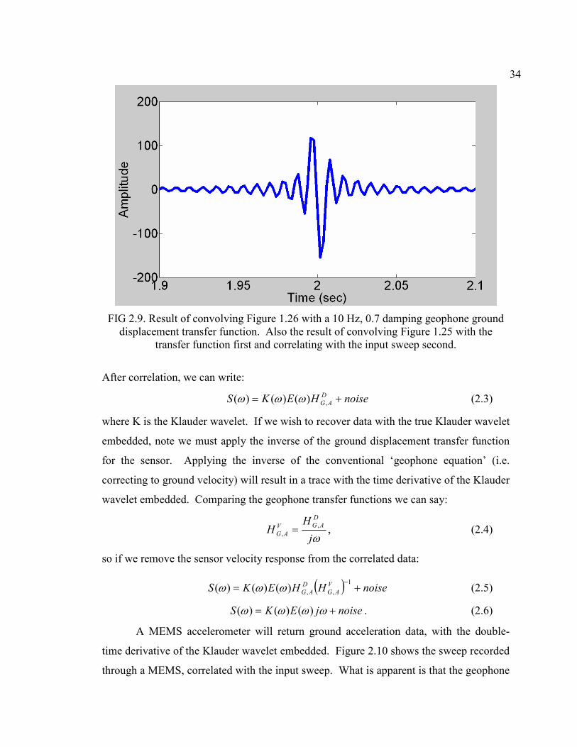
34

FIG 2.9. Result of convolving Figure 1.26 with a 10 Hz, 0.7 damping geophone ground

displacement transfer function. Also the result of convolving Figure 1.25 with the

transfer function first and correlating with the input sweep second.

After correlation, we can write:

noiseHEKS D

AG += ,)()()( ωωω (2.3)

where K is the Klauder wavelet. If we wish to recover data with the true Klauder wavelet

embedded, note we must apply the inverse of the ground displacement transfer function

for the sensor. Applying the inverse of the conventional ‘geophone equation’ (i.e.

correcting to ground velocity) will result in a trace with the time derivative of the Klauder

wavelet embedded. Comparing the geophone transfer functions we can say:

ωj

HH

D

AGV

AG

,

, = , (2.4)

so if we remove the sensor velocity response from the correlated data:

( ) noiseHHEKS V

AG

D

AG +=−1

,,)()()( ωωω (2.5)

noisejEKS += ωωωω )()()( . (2.6)

A MEMS accelerometer will return ground acceleration data, with the double-

time derivative of the Klauder wavelet embedded. Figure 2.10 shows the sweep recorded

through a MEMS, correlated with the input sweep. What is apparent is that the geophone

35

and MEMS operate on the Klauder wavelet the same as they did on the minimum phase

wavelets. This means that the geophone-to-MEMS transfer equation derived in Section

1.3 will apply and correctly calculate data equivalent to one sensor from the other.

FIG 2.10. Sweep recorded through accelerometer, then correlated with input sweep. The

result matches with the double time derivative of the Klauder wavelet.

2.4 Spiking deconvolution

More practical modeling will be undertaken by convolving a wavelet with a

reflectivity series, then convolving the resulting trace with a sensor response and finally

attempting a simple deconvolution. Wiener, or spiking, deconvolution will be used. It

inherently assumes a stationary, minimum phase embedded wavelet and a white

reflectivity amplitude spectrum. These assumptions are approximate met here.

Figure 2.11 shows the reflectivity series that will be used to create the synthetic

seismograms. It was generated using the reflec.m utility in the CREWES Matlab

toolbox. Its spectrum is shown in Figure 2.12. The spectrum does not really fit the label

of ‘white’, but neither does it show any particular tendency to be weighted ‘red’ or ‘blue’.

It approximately meets the assumption of spiking deconvolution, and should not

advantage one sensor over another.

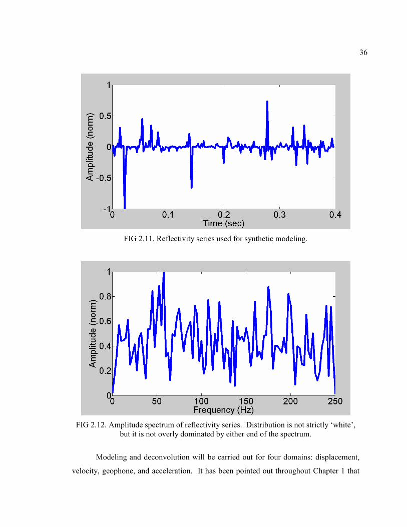
36

FIG 2.11. Reflectivity series used for synthetic modeling.

FIG 2.12. Amplitude spectrum of reflectivity series. Distribution is not strictly ‘white’,

but it is not overly dominated by either end of the spectrum.

Modeling and deconvolution will be carried out for four domains: displacement,

velocity, geophone, and acceleration. It has been pointed out throughout Chapter 1 that

37

while the amplitude spectra of analog geophone output and ground velocity are similar,

the differences at low frequencies and in phase make them very different domains. The

wavelets were created with the WaveletEd utility in the CREWES Syngram package.

The four wavelets are shown in Figure 2.13, and their amplitude spectra are in Figure

2.14. Since the acceleration wavelet is at a maximum around the same frequencies (~50

Hz) as the reflectivity, it might be predicted that the acceleration trace would be at an

advantage in the deconvolutions. The synthetic seismograms were created by convolving

the displacement wavelet with the reflectivity series and then performing the

differentiation or sensor response convolution in the frequency domain. However, since

the order of convolution does not matter, this is equivalent to convolving each of the four

wavelets with the reflectivity. Figure 2.15 shows the ground displacement and velocity,

with the reflectivity series for comparison. Figure 2.16 shows the geophone and

acceleration domains, again with the reflectivity.

FIG 2.13. Wavelets used in modeling. Impulsive source displacement (25 Hz): blue

circles. Ground velocity: green squares. Ground acceleration: red triangles. Raw

geophone output: purple stars.

38

FIG 2.14. Amplitude spectra of wavelets in Figure 2.13.

FIG 2.15. Ground displacement (green) and velocity (red) for a 25 Hz minimum phase

impulsive displacement wavelet, with reflectivity series (blue).

39

FIG 2.16. Geophone output trace (purple) and ground acceleration (orange), for a 25 Hz

minimum phase impulsive displacement wavelet, with reflectivity (blue).

The results from the spiking deconvolutions are shown in Figures 2.17 and 2.18.

The displacement and velocity traces gave the best deconvolutions, though all results

were similar. Crosscorrelations showed that the maximum value was for the velocity

input, with 0.674. Next was ground displacement (0.658), then the geophone trace

(0.622), and finally the acceleration trace (0.600). While these results suggest correcting

to velocity (by dephasing geophone data or integrating MEMS accelerometer data) may

provide better deconvolution, this may be due the particular amplitude distribution of this

example. It can be interpreted as a confirmation that low frequencies are extremely

important to deconvolutions. Certainly the geophone and acceleration traces yielded very

similar results. In field data, a full processing flow with several passes of deconvolution

yield little to no difference in the final section (Hauer, 2008, pers. comm.; Stewart, 2008,

pers. comm.).

40

FIG 2.17. Spiking deconvolution results for ground displacement (green) and velocity

(red), with the true reflectivity (blue).

FIG 2.18. Spiking deconvolution results for the geophone trace (purple) and the ground

acceleration trace (orange), with true reflectivity (blue). The results are similar to each

other, but generally poorer than those in Figure 2.17.

41

The robustness of each domain in the presence of noise was investigated to see if

one had any significant advantage over the other. First, random noise with a uniform

distribution was added to the ground displacement trace at varying levels, and the

resulting traces were deconvolved, again with a spiking deconvolution. This was

intended to model harsh, random noise in the field due to actual vibrations associated

with wind and shocks. Noise was added at 80, 60, 40, 20, 10, 5 and 3 dB down relative

to the largest amplitude in the ground displacement trace. The ground displacement trace

was then filtered appropriately in the frequency domain to yield ground velocity and

acceleration traces, and a geophone trace. These were then sent independently into

deconvolution. The maximum crosscorrelation value was recorded and plotted. The

results are shown in Figure 2.19. We see that none of the domains enjoys a remarkable

edge over the others, and it can’t reasonably be concluded that any domain is more robust

against field noise.

0

0.1

0.2

0.3

0.4

0.5

0.6

0.7

0.8

0 20 40 60 80 100

Noise amplitude (dB down)

Deconvolution xcorr

Displacement

Velocity

Geophone

Acceleration

FIG 2.19. Correlation to the reflectivity model after spiking deconvolution. Different

random noise amplitudes, added to the ground displacement.

42

The same analysis was undertaken, but introducing the same noise into each trace

after it had been ‘recorded’ (i.e. transformed into the appropriate domain). This is an

approximation of recording system noise, presumed here to be white. The results are

shown in Figure 2.20. Again we see little to choose between the domains, especially at

higher noise amplitudes (10 dB down and above), where the similarity between the four

results suggests the noise is contributing more than the recorded signal. Certainly a

deconvolved trace that is less than 40% correlated with the reflectivity is not

interpretable.

0

0.1

0.2

0.3

0.4

0.5

0.6

0.7

0.8

0 20 40 60 80 100

Noise amplitude (dB down)

Deconvolution xcorr

Displacement

Velocity

Geophone

Acceleration

FIG 2.20. Correlation to the reflectivity model after spiking deconvolution. Different

random noise amplitudes, added to the recorded trace.

LABORATORY TESTING

Sensor testing in a lab setting was undertaken to determine if geophones and

MEMS conform to the theoretical responses in Chapter 1. This work was performed by

the Velocity and Acceleration Sensor Testing and Analysis (VASTA) project at the

43

University of Calgary, conducted jointly by the Mechanical and Manufacturing

Engineering Department and the Geoscience Department, under the direction of Dr.

Swavik Spiewak and Dr. Robert Stewart. The creation of a state of the art seismic test

facility was in part sponsored by industry partner ARAM Systems Ltd. of Calgary,

Alberta. All figures presented here were generated from VASTA results using programs

written by Dr. Spiewak and Wenyu (Winston) Liu, a Ph. D. student in Mechanical and

Manufacturing Engineering.

As stated earlier, sensor testing is largely concerned with defining an input to the

sensor and measuring the output to determine transfer characteristics. Testing of

geophones is often performed by feeding pulses or square waves of current back through

the coil, and measuring the response that follows. This provides a very precise input with

which to characterize the sensor. However, there is no simple means to apply such a

method to a seismic-grade MEMS accelerometer, which outputs a digital signal. When

feedback is used in a MEMS accelerometer, there would need to be direct access to the

feedback loop in order to apply a current impulse. Immediately after the current impulse

the access would have to be removed so it does not interfere with the resulting response.

In practice this would be very difficult to achieve.

The only method readily available is to set up an extremely precise vibration

table, and physically shake the sensors to compare their responses. Testing with this

method is trying, as it becomes essential to determine to what extent deviations from the

modeled sensor response are due to nonlinearities in the sensor, and to what extent they

are due to nonlinearities in the test equipment. If it is determined the test equipment

cannot be made accurate to below the sensors’ noise floor, then characterization and

correction for the equipment nonlinearity is necessary. Ambient noise also becomes a

larger problem as input amplitudes decrease. Considering that seismic sensors are

designed to rank among the most sensitive and lowest noise sensors in the world,

ensuring that the test input is even more precise is a challenging subject.

To eliminate as much ambient noise as possible, the lab was located in the

basement of the Petro-Canada Mechanical and Manufacturing Engineering building, in a

corner by two load-bearing walls. Sources of ambient vibrations within the test room

44

were minimized. The apparatus was placed on a heavy, granite-slab table, on both

passive and active vibration isolation surfaces. Each vibration isolation surface was

monitored with a very low-noise accelerometer, and the motion of the stage itself was

monitored with a laser interferometer. Tests were performed at night or on weekends,

when traffic and other city noise was at a minimum, and ambient noise was generally less

than 500 ng/√Hz (Figure 2.21), from 1 Hz up to nearly 100 Hz. This was measured by a

low noise seismometer on the active vibration isolation table (red line) and a geophone

(blue line). This gives a noise floor of about 7 µg over a 200 Hz bandwidth, or 1.1 µm/s

at 10 Hz.

FIG 2.21. Noise spectra recorded during a quiet weekend period (Sunday, 9am).

There were two vibration patterns used in VASTA. The first was a single

frequency sinusoid, repeated at many frequencies to find the observed amplitudes and

phase lags. This is referred to as ‘harmonic scan’ analysis. Fitting a model (in a least-

squares sense) based on the theoretical transfer function to the observed data points

allowed an estimation of the sensor parameters (resonance, damping and gain constant),

and comparison to manufacturers’ specifications. After the electrical impulse response

method, this is the most common method used to characterize sensors.

The second, and potentially more realistic, pattern was to use a set of vibrations

with a Gaussian distribution about some desired amplitude (usually defined in

45

displacement) but with a ‘white’ amplitude spectrum, so all frequencies are considered

over the test interval. There are a few different methods of determining the sensor

parameters from these data, some with advantages over others. They are beyond the

scope of this work, however, and only the harmonic scan results will be discussed here.

Full test reports were produced for 4 Oyo Geospace GS-32CT horizontal

elements, 2 Oyo Geospace GS-42 omnidirectional elements and 1 AppliedMEMS (now

Colibrys) SiFlex 1500S accelerometer. The results from the harmonic scans are shown in

Table 2.1. All tested sensors are very close to the manufacturer’s quoted values, and with

only one exception are within quoted error bounds.

Table 2.1. Comparison of quoted and tested sensor parameters

Element GS-32CT

GS-32CT

GS-32CT

GS-32CT

GS-42

GS-42

GS-42

GS-42 SF1500 SF1500

Sensitivity Vs/m 27.5 27.5 27.5 27.5 22 22 22 22 1.192 1.192

Tested sensitivity Vs/m 28.2 27.7 27.6 27.6 22.2 22.2 22.7 22.7 1.199 1.229

Resonance Hz 10 10 10 10 15 15 15 15

Tested resonance Hz 10.05 9.9 9.83 9.9 15.05 14.99 15.42 15.35

Damping dim 0.316 0.316 0.316 0.316 0.68 0.68 0.68 0.68

Tested damping dim 0.306 0.315 0.311 0.311 0.672 0.654 0.656 0.641

Table 2.2. Quoted error bounds of tested sensors

Oyo Geospace GS-32CT Oyo Geospace GS-42 SiFlex 1500

All specs plus/minus 2.5% resonance plus 10% to minus 5% linearity 0.10%

sensitivity plus/minus 5% No sensitivity spec

damping plus 10% to minus 15%

2.5 Vertical orientation

There were two ranges of amplitudes applied in the vertical tests: one moderate

and one extremely weak. The moderate amplitudes were defined as between 500 and

5000 µm/s, while the extremely weak amplitudes were below 10 µm/s. Significant

efforts were made to measure and account for any imperfections in the input sinusoids.

46

Full reports were completed for two sensors in the vertical orientation: two

geophones (both model GS-42), and one accelerometer (Colibrys SiFlex 1500). At the

time the tests were undertaken, a low-noise, ∆Σ-based MEMS accelerometer comparable

to those used in the digital seismic sensors was not commercially available. The SiFlex

1500 is an analog feedback MEMS accelerometer, with a noise floor an order of

magnitude higher (~300 ng/√Hz) than that quoted for seismic-grade accelerometers (~30

ng/√Hz). The SiFlex also has a significantly higher maximum input acceleration (3 g)

than field digital seismic sensors (~1.2 to 1.5 g).

Medium Vibration

An example test result from the harmonic scan is shown in Figure 2.22. The red

dots are the recorded magnitude, and the grey line is the model fit to those points by

least-squares. This is the GS-42 geophone response to strong vibration amplitudes. The

amplitude of each tested sinusoid in µm/s is shown in Figure 2.23. It is apparent that the

response of the geophone lies very closely along the fitted model. Also, the fitted model

agrees very closely with the manufacturer’s model.

FIG 2.22. Harmonic scan results for geophone GS-42.

47

FIG 2.23. Medium strength vibration amplitudes for the harmonic scan. Left – geophone,

right – MEMS.

The sensors will be compared by examining plots of the differences between the

fitted model and the observed points. The fact that the estimated parameters were all

within the error bounds shows that the geophones are operating as expected in general, so

more specific trends concerning different frequency bands will be explored. Comparison

of Figures 2.25, 2.26 and 2.27 shows that all sensors have very small deviations in

general. It appears that the MEMS is outperforming the geophone at low frequencies.

This observation is somewhat false, as Figure 2.24 shows the amplitude of the vibration

was slightly larger at low frequencies during the MEMS test than the geophone test.

Taking this into account, there still appears to be some advantage for the MEMS at the

very lowest frequencies (at and below 1 Hz), where the geophone’s amplitude and phase

responses become somewhat unreliable. At high frequencies both sensors perform well,

with amplitude and phase deviations less than 0.5 dB and 5 degrees, respectively. The

MEMS may also be showing some advantage at very high frequencies (more accurate

amplitudes), which is expected since acceleration is larger than velocity by a factor of ω.

Again the vibration amplitude was larger for the MEMS than the geophone, but both are

large enough that the sensors should have no difficulty picking them up.

FIG 2.24. Velocity of medium vibrations. Left – geophone, right – accelerometer.

48

Figure 2.25. Deviations from model, SF1500 accelerometer, medium vibrations.

FIG 2.26. Deviations from model, GS-42 geophone, medium vibrations.

FIG 2.27. Deviations from model, second GS-42 geophone, medium vibrations.

Ultra weak vibration

The tests were repeated using much weaker vibrations (Figure 2.28), and the

deviations from the model are shown in Figures 2.29, 2.30 and 2.31. At low frequencies,

(<10 Hz) the magnitude of the vibrations agrees very closely in both tests. Both sensors

seem to run into difficulty just below 10 Hz, which corresponds to an input of ~0.6 µm/s,

or ~3.8 µg. The MEMS appears to have less deviation in amplitudes below 10 Hz, but its

phase is totally unreliable and for both sensors the output would not be distinguishable as

49

signal in real seismic data. The fact that both sensors fail very close together suggests

this may represent the useable noise floor of the test equipment in its present state. It is

impressive that both sensors are within a few dB and a few degrees of their expected

response at vibration amplitudes well below 10 µg.

FIG 2.28. Velocity of ultra weak vibrations. Left – geophone, right – MEMS.

FIG 2.29. Deviations from model, SF1500 accelerometer, ultra weak vibrations.

FIG 2.30. Deviations from model, GS-42 geophone, ultra weak vibrations.

50

FIG 2.31. Deviations from model, GS-42 geophone, second test, ultra weak vibrations.

2.6 Horizontal orientation

The tests were repeated in horizontal configuration. The GS-42 geophone and the

SiFlex 1500 MEMS are omnidirectional, so the same elements were used as in the

vertical orientation.

Strong vibration

As shown in Figure 2.32, these were very strong vibrations, over 12 mm/s. The

strongest peak acceleration for the geophone was about 0.38 g (at 60 Hz), and for the

MEMS was about 0.58 g (at 70 Hz). Under the strongest vibrations both sensors were

again very near their modeled response, within a few tenths of a dB and a few degrees

phase lag. However, at higher frequencies the geophone (Figure 2.34, 2.35) deviates

from its modeled phase significantly, even though the vibration amplitude has decreased

significantly. The fact that the MEMS shows only a slightly greater deviation at high

frequencies than low frequencies (Figure 3.33) suggests it is not the vibration plane that

is responsible. This deviation from the model by the geophone suggests some manner of

frequency dependence in a parameter: either decreasing spring force at higher frequency,

or decreased damping. These deviations are not observed, however, in the closer

tolerance GS-32CT geophones (Figure 2.36).

51

FIG 2.32. Velocity of strong vibrations. Left – geophone, right – MEMS.

FIG 2.33. Deviations from model, SF1500 accelerometer, strong vibrations.

FIG 2.34. Deviations from model, GS-42 geophone, strong vibrations.

FIG 2.35. Deviations from model, GS-42 geophone, second test, strong vibrations.

52

FIG 2.36. Deviations from model, GS-32CT geophone, strong vibrations.

Weak Vibration

The horizontal vibration table was not capable of accurately producing ultra weak

vibrations, so these are larger than for the vertical setup (Figure 2.37). Again, we see the

GS-42 element encounters larger phase errors (Figure 2.39, 2.40) at high frequencies than

the SiFlex accelerometer (Figure 2.38). It appears the source of these deviations is

frequency dependent, and amplitude independent. As above, the GS-32CT does not

exhibit the problem as badly (Figure 2.41).

In any case, a very wide range of amplitudes was tested in the horizontal

orientation, and all sensors performed to within a half a dB in amplitude and a few

degrees in phase of their modeled response, with a few exceptions. Clearly both

geophones and MEMS accelerometers operate as expected, over a wide range of

frequencies and amplitudes.

FIG 2.37. Velocity of weak vibrations. Left – geophone, right – accelerometer.

53

FIG 2.38. Deviations from model, SF1500 accelerometer, weak vibrations.

FIG 2.39. Deviations from model, GS-42 geophone, weak vibrations.

FIG 2.40. Deviations from model, GS-42 geophone, second test, weak vibrations.

FIG 2.41. Deviations from model, GS-32CT geophone, weak vibrations.

54

Chapter III: VIOLET GROVE FIELD DATA

3.1 Experimental design

Field data were acquired in December, 2005 near Violet Grove, Alberta, Canada

in the Pembina oil field. A detailed description of the acquisition can be found in Lawton

et al. (2006). Three sensors (two 3C geophones and one Sercel DSU3 MEMS) were

simultaneously laid out at 8 stations, with a separation of ~1 m from each other and 20 m

receiver station spacing. One geophone (ION Spike) was a nail-style case that places the

sensor elements below the surface, and the other (Oyo 3C) was a surface-style case with

the sensor elements within a container sitting on the surface, coupled to the earth with a

long spike. A third geophone was also located at two of the stations, and was also a nail-

style case (Oyo Nail) (Figure 3.1). Some parameters of the sensors can be found in Table

3.1. The layout geometry is shown in Figure 3.2.

The intention was to test different methods of coupling the sensors to the ground

(different geophone case designs), as well as differences between geophones and MEMS-

based DSU3 sensors. The ground was solidly frozen when the sensors were laid out, and

warm water was used to soften the earth so the sensors could be planted. The sensors

then froze into the earth after planting so coupling was generally excellent. The two

geophones will thus be considered as indicative of what degree of variation is expected

due to the 1 m crossline offset. This includes small differences in ambient noise,

coupling conditions, raypaths through the near surface, and other issues related to the

sensors not being exactly collocated. If the variation between the accelerometer and

geophone records is not greater than the variability between two geophone records, it will

be concluded that the difference between the accelerometer and the geophones is not

significant. Some noise difference between the surface geophone and the nail-style

geophones will be seen later, but in the time domain the geophones are extremely similar

(Figure 3.3). The overall excellent coupling resulted in very wide bandwidth being

recorded, which allows a good analysis of the abilities of each sensor at the low and high

ends of the spectrum.

55

A total of 222 dynamite shots were recorded, whose locations are shown in Figure

3.2. The MEMS data were corrected for tilt prior to delivery, while the geophone data

were not. All sensors were carefully leveled in the field, however, and experimentation

with mixing vertical and horizontal geophone traces to approximate tilt angles up to 15

degrees found the effect of reasonable tilts to be negligible. The vertical components of

the sensors showed exceptional similarity especially between geophones, and also

between geophones and MEMS. Crosscorrelation coefficients between the geophones

were above 0.99 (Figure 3.3, Lawton et al., 2006). The following analysis will focus on

receiver gathers from shot line 1, where the sensors were always separated from the shots

by nearly 100m, and shot line 3, where station 5190 lies on the shot line.

Table 3.1. Parameters of sensors and cases at Violet Grove

Field Case Spike GS-3C Nail DSU

Sensor Element SM-24 GS-20DM

GS-32CT MEMS

Resonance Hz 10 10 10 >800

Damping 0.69 0.7 0.7 N/A

Sensitivity w/ damping Vs/m 20.5 19.7 19.7 N/A

Proof mass g 11 8 11.2 <<1

Max excursion mm 2 2 1.52 <<1

Spurious resonance Hz 240 300 250 >>800

Depth of penetration (est) in 4.8 3.13 6 5.625

Figure 3.1. The three geophone cases used in the sensor test. Left: Oyo 3C, middle: ION

Spike, right: Oyo Nail.

56

FIG 3.2. Survey design. Blue points are shots recorded in the experiment and red points

are recording stations (Lawton et al., 2006).

FIG 3.3. Trace by trace comparison of raw Violet Grove data (Lawton et al., 2006). Red

– Oyo Nail, Blue – ION Spike, Green – Oyo 3C, Orange – Sercel DSU.

57

3.2 Recording Instruments

i. Anti-alias filters

Two different recording instruments were used: an ARAM Aries system for the

geophones and a Sercel 408UL system for the DSU3 units. The geophones were sampled

at 1 ms, while the DSU3s were sampled at 2 ms. The only other difference applied by the

recording instruments is the geophones (connected to the ARAM system) used zero-

phase anti-alias filter (AAF) (Figure 3.4) while the Sercel (408UL) system used a

minimum-phase AAF (Figure 3.5). Lawton et al. (2006) suggested that this may have

introduced phase effects into the data, resulting in the raw geophone traces appearing

more similar to the raw MEMS traces than was expected. Their reasoning was that

causal filters have a strongly non-zero phase response, even through the seismic data

band. Figure 3.5 shows that for the causal filter used in the Sercel recorder, the

amplitude response is flat up to 200 Hz and the filter phase response is strongly nonzero

at all frequencies above ~1 Hz. On a linear frequency scale, the phase lag is linear up to

over 100 Hz. The result of applying a filter with a flat amplitude response and linear

phase response is a simple time delay (Telford et al., 1977), as all frequencies are delayed

a proportional amount that maintains the waveform intact. Thus no substantial change to

the waveform is expected from the antialias filter in the 0-100 Hz range. The reason the

geophone and MEMS records are similar is explained in section 2.1.

FIG 3.4. Antialias filter parameters for geophones (ARAM). Left: amplitude. Right:

Phase.

58

FIG 3.5. Antialias filter parameters for DSU.

Figure 3.6 shows a 30 Hz Ricker wavelet sampled at 0.1 milliseconds. As shown

in Figure 3.7, the result of downsampling to 2 milliseconds with the causal filter from

Figure 3.5 is a time delay of a little over 6 ms, with no perceptible phase distortion. A

Ricker wavelet has a relatively narrow band of frequencies, but covers most of the

dominant frequencies in field data. Above ~100 Hz, the phase response of the causal

AAF can no longer be assumed to be linear, and it will begin delaying these higher

frequencies beyond the proportional amount. This agrees with another conclusion of

Lawton et al. (2006), that the tendency of high frequencies to trail the main peak in the

Sercel DSU3 data is partly attributable to its AAF.

FIG 3.6. Ricker wavelet, fdom=30 Hz, sampled at 0.0001 seconds.

59

FIG 3.7. Figure 3.6 downsampled to 0.002 seconds using the filter in Figure 3.5. Phase

effects are barely perceptible, except for a constant time shift of a little over 6 ms.

For comparison of the field data in the time domain, the minimum phase AAF is

replicated in the (1ms) geophone data by downsampling to 2ms with a minimum phase

filter. The filter had a corner frequency of 0.82 Nyquist (205 Hz), with 120 dB rejection

at Nyquist. Replicating the filter should replicate the time shift and any peripheral phase

effects. The DSU3 data could, equally, be inverse filtered to remove the time shift and

phase effects (Figure 3.8). Note also in Figure 3.4 that the ARAM system uses a 3-Hz

low-cut filter while the DSU-408 has none. This too was replicated by applying an

equivalent low-cut filter to the DSUs. From here on all ‘raw’ DSU traces in this dataset

have, in fact, been low-cut filtered to match the ARAM system.

FIG 3.8. Result of applying inverse AAF to the downsampled result in Figure 3.7.

60

ii. Pre-Amp gain and scaling

There is no quoted pre-amp gain for the Sercel DSU3-408UL, as the digitization

takes place within the sensor and no settings can be selected. In the ARAM Aries,

however, there is a choice of a 12, 24 or 30 dB pre-amp gain. These have a bearing on

the equivalent input noise added by the digitizing box, and on the maximum voltage

before clipping. From inspection of the only receiver gather that lies on a shot line

(station 5190, shot line 3; Figure 3.9), it is observed that the geophone values are clipped

at approximately 0.21. This clipping is observed in the raw SEG-Y numerical values,

and is not a result of the display parameters. With a pre-amp gain of 24 dB, the

maximum voltage before clipping is 0.214. However, it can also be seen by comparing

numerical values at specific samples within the gathers that the amplitudes in the ION

Spike data are double those of the Oyo GS-3C. If the ION Spike gather was in fact

gained by 30 dB, the extra 6 dB would account for the doubling of the amplitudes. It is

thus interpreted that the digitizing box, forced to record from different pre-amp gains on

adjacent channels (Figure 3.10), recorded all amplitudes as if both channels were a 24 dB

preamp gain. As a result, the Oyo GS-3C gather exhibits the correct values in volts, but

the ION Spike gather should have its amplitudes halved to correctly represent the value in

volts that went into the digitizing box. The Oyo Nail, present at stations 5183 and 5184,

also needs to be halved in amplitude.

Chapter 1 shows that once an acceleration trace has been calculated from a

geophone voltage trace, the amplitudes should be divided by the geophone’s damped

sensitivity constant to give actual ground acceleration values. For the sensor elements

used here, their damped sensitivities are given in Table 3.1.

61

FIG 3.9. Spike closeup of station 5190, shot line 3, raw geophone data. Centre 4 traces

are clipped, surrounding traces approach similar values.

FIG 3.10. Diagram of gain settings on the ARAM field box.

Comparison of these calculated acceleration amplitudes to the acceleration

records from the DSU, however, showed the DSU amplitudes being too small. The

record for station 5190, line 3 also contained clipped traces for the DSU. The DSU

specifications stated a maximum acceleration of 4.5 m/s2, or 0.459 g. The clipped values

in the DSU SEG-Y file were around 2300. The idea of 1 amplitude unit from the DSU

equaling 2 mm/s2 was explored, but did not produce amplitudes in the neighbourhood of

those from the geophones. Thus, there becomes a discrepancy about which numerical

value of acceleration should be trusted. Since the acceleration calculated from the

geophone traces was in known units (m/s2), while the DSU brochure does not specify

what the output units are, I elected to match the DSU amplitudes to the geophone rather

than the other way around.

62

Trial and error found that multiplying the DSU values by .00125 produced a very

good fit overall, generally placing the dominant amplitudes of the DSU within the range

of the dominant amplitudes from the geophones. This scaling constant (1 DSU amplitude

unit equals 1.25 mm/s2) was found to work under all conditions, from the smallest

amplitudes to the largest, and in both vertical and horizontal orientations. Figures 3.11

and 3.12 show amplitude spectra from station 5183, line 1, from the final 500 ms and the

full 4000 ms, respectively. The final 500 ms may be expected to have the smallest

amplitudes and little source energy, while the spectra for the full 4000 ms will be

dominated by the strongest amplitudes in the near offset traces and the first breaks. In

both cases the MEMS spectrum is within 1 dB of the geophone spectra, and within the

variation between geophones. Perhaps the greatest difference in amplitudes is found

again at station 5190, line 3. The last trace is from a source over 1.5 km away, while

traces 44 and 45 are immediately adjacent to the shot and are clipped (Figure 3.13).

Figure 3.14 shows the amplitude spectra from the bottom two seconds of the last trace in

the receiver gather (farthest from the shot). The empirical scaling puts the DSU

amplitudes in between the geophones. Figure 3.15 shows the spectra from trace 47, and

it is clear that as soon as the amplitudes decrease from the clipped value, the

accelerometer very closely matches the geophones again. The largest amplitude in trace

47 is about 92% of the largest amplitude in trace 45, so the accelerometer and the

geophone match along almost all of the accelerometer’s unclipped range.

The largest accelerations in the far offset trace (trace 73) are more than 50 dB

(300 times) smaller than those in the near offset trace (trace 47), but the same scaling

constant works for both. This is good evidence that both sensors are linear over a very

wide range of amplitudes.

63

Figure 3.11. Amplitude spectra, station 5183, line 1, 3500 to 4000 ms.

Figure 3.12. Amplitude spectra, station 5183, line 1, 0-4000 ms.

64

FIG 3.13. Sercel DSU3 closeup of station 5190, shot line 3, raw MEMS data. Center 2

traces (44 and 45) are clipped, and adjacent traces (43 and 47) contain similar values.

FIG 3.14. Comparison of spectra from station 5190, line 3, trace 73, >2000 ms.

65

FIG 3.15. Comparison of spectra from station 5190, line 3, trace 47.

iii. Noise floors

Comparison of noise floors is discussed in a theoretical example in Chapter 1. In

these field data, the geophone recorder was set to sample at 1 ms, while the DSU3 system

recorded at 2ms. As both recorders use ∆Σ digitizers (described in Chapter 1), and a

faster sampling rate means greater digitizing noise in a seismic sample, this means the

equivalent input noise specifications for the geophones and DSU3s are, ironically, not

equivalent. For this kind of system, halving the quoted sample rate will double the noise

(Figure 3.16). This may help make noise floor differences between geophones and

accelerometers more apparent, particularly at high frequencies. Given that the GS 3C

was preamp gained 24 dB (0.4 µV EIN @ 1 ms sampling), while the Spike and Nail were

gained 30 dB (0.32 µV EIN @ 1 ms sampling), an estimate of the expected noise floors

based on manufacturer’s specifications is shown in Figure 3.17. The DSU noise floor is

expected to be lower above ~70 Hz, while the geophone noise should be lower below.

66

Error in a delta signal loop

y = -0.98x + 6.44

-8

-6

-4

-2

0

2

4

6

8

0 2 4 6 8 10Log2(samples)

Log2(error(%))

FIG 3.16. Error magnitude in a ∆Σ loop with increasing loop iterations. The slope of

nearly -1 shows that doubling the samples averaged halves the error in the output value.

-130

-120

-110

-100

-90

-80

-70

-60

1 10 100 1000

Frequency (Hz)

Noise amplitude (dB - m/s^2)

ION Spike & OYO Nail

DSU3-408

OYO 3C

Low Noise Model

High Noise Model

FIG 3.17. Modeled noise floors of the two field recording instruments, and estimated

range of ambient noise.

This noise floor will only be significant if it is above the ambient noise detected

by the sensor. This is unlikely to be the case over frequencies where the geophone noise

floor is lowest, particularly at resonance, where it dips nearly to 100 ng. The New Low

Noise Model (Peterson, 1993), used by earthquake seismologists, suggests a minimum

67

noise floor of about 50 ng over a 250 Hz band, for a borehole seismology station. The

most comparable North American station that contributed to that study (Black Hills,

North Dakota) shows a noise floor over a 250 Hz band of about 500 ng. This figure is

from a near-surface seismic vault, certainly a quieter environment than might be expected

in a normal exploration survey. The high noise estimate is nearer to 500 µg (500 000 ng),

and, considering the data collection in this thesis was undertaken in an operating oilfield

with nearby noise sources, it is conceivable that the ambient noise could be nearer to that

upper limit.

3.3 Vertical component data

As there were many more shots than receivers, only receiver gathers will be

considered. All data will be compared in the acceleration domain. This ensures that

there is no worry about minimizing or losing anything from the MEMS data. In other

words, it allows the examination of whether ground acceleration comparable to that

acquired with a MEMS accelerometer can be calculated from geophone data. The DSU

case has the vertical component sensor element near the bottom of the nail section, and so

it will be compared mostly to the Spike geophone, which was the closest nail-style

geophone. An example receiver gather through a geophone is shown in Figure 3.18, and

through the MEMS sensor is Figure 3.19.

FIG 3.18. I/O Spike receiver gather, station 5183, 500 ms AGC applied.

68

FIG 3.19. Sercel DSU3 receiver gather, station 5183, 500 ms AGC applied.

A trace-by-trace comparison (Figure 3.3) (Lawton et al., 2006) shows that

geophone and MEMS data are fairly similar, with the main distinguishing feature in the

DSU3 record being a small time shift (related to the minimum phase AAF) and some

added high frequency character. This additional high frequency content in the

accelerometer gather (compared to the raw geophone gather) is not unexpected, as in

Chapter 1 it is explained that the amplitude spectrum of MEMS sensors is flat in

acceleration, while the amplitude spectrum of a geophone is flat in velocity above

resonance (taking a time derivative adds 6 dB per octave to an amplitude spectrum).

i. Amplitude Spectra (Global)

Examining the data in the frequency domain allows the easy comparison of the

different sensors at a station at once. The average amplitude spectra of the acceleration

domain records (ION Spike acceleration, Oyo Geospace 3C acceleration, Oyo Geospace

Nail acceleration and DSU3 raw) will be examined first. For each receiver gather, an

amplitude spectrum was calculated for each trace, and these were averaged to give the

result. The result is that these spectra will be dominated by the section of the gather with

the largest amplitudes: early arrivals on the centre traces.

Shown in Figure 3.20 is Station 5183, shot line 1. Figure 3.21 shows the shots

from shot line 3 into the same station. From 5 Hz up to ~40 Hz, the acceleration spectra

are nearly identical. Below 5 Hz the curves are significantly different, and from the

69

laboratory results in Chapter 2 it might be suggested that the DSU3 is closer to the correct

amplitudes at the very lowest frequencies.

FIG 3.20. Average spectra from all four sensors at station 5183, shot line 1.

FIG 3.21. Average spectra from all four sensors at station 5183, shot line 3.

Figure 3.22 shows a closer view of the frequencies below the dominant frequency

of the data. At low frequencies (below geophone resonance), the strong similarities

70

between the calculated acceleration (from the geophone gather) and the measured

acceleration (from the raw DSU3) suggest there is little improvement in low frequency

data quality using a MEMS-based sensor instead of a geophone. This does not

necessarily represent a failure of the MEMS sensor, but is in my view more of a

validation of the position of Brincker et al. (2001) that frequencies of at least an octave

below geophone resonance are recorded accurately and can be used to provide valuable

information. If the goal is lithologic estimation (especially impedance inversion), these

low frequency amplitudes should probably be included as long as there is reason to

believe source-generated signal exists in that band. Since there is necessarily a decreased

emphasis on low frequency content in acceleration data, a case may be made for using

velocity or displacement domains (e.g. integrating MEMS-recorded data) if they is to be

used in seismic inversion.

FIG 3.22. Closeup of average spectra from station 5183, line 1, 0-25 Hz.

In Figure 3.20, the higher frequencies show considerable differences between the

three geophones (which are similar to each other), and the MEMS. Data from the other

stations can be used to see if these differences are consistent across stations, or related

specifically to one station. Figures 3.23 to 3.29 show the global average amplitude

spectra for the other seven stations (top shows shot line 1 and bottom shows shot line 3).

71

The differences observed at frequencies greater than the dominant frequency are not

consistent over all stations, while the similarity in the low frequencies is consistent. At

some stations, like 5189, no differences are apparent. At others, like 5188, the MEMS

amplitudes above ~80 Hz are larger than the geophones (opposite to station 5183).

Viewing the spectra from shot line 3, we see that the patterns are consistent with

station number. At station 5183, shot line 1 has a similar appearance to shot line 3, and

this is generally true of all the stations. It is not true of station 5190 because this is where

the shot line intersected the receivers, and all of the records suffered from clipping, albeit

at different values for the MEMS and geophones. Note that the clipping has mostly

appeared to affect the relative values at low frequencies, and is less significant at high

frequencies. The most readily available explanation for station-specific patterns is that

they are related to the coupling of the sensors with the ground. As noted in Table 3.1, the

different sensors penetrate to different depths into the soil. The fact that water was used

to soften the earth may be producing the differences in coupling observed. Varying

permeability of the soil combined with penetration depth of the sensor could produce a

wide range of coupling conditions, varying even between the vertical and horizontal

components.

Finally, a fully global amplitude spectrum was calculated using all unclipped

traces from all of the stations and shots (lines 1 and 3). The OYO Nail was not present at

all stations and is not included. This should provide a good overall idea of the effective

response differences between the datasets. Differences that appear consistently and

strongly will be apparent; differences that are weak or inconsistent will average out.

Where the spectra overlie each other, the sensors worked according to their modeled

response. Differences represent consistent deviations from the modeled response. Figure

3.30 shows that once all traces are averaged, the geophones are virtually identical to each

other, suggesting there is no consistent difference between them in large amplitude

events. The DSU spectrum also matches extremely well from 5 Hz up to ~120 Hz. At

frequencies higher than this, the DSU amplitudes are consistently smaller. It is unclear

whether this is due to the coupling between the DSU case and the earth, or a tendency of

the sensor element itself.

72

FIG 3.23. Average amplitude spectra, station 5184: top) shot line 1, bottom) shot line 3

FIG 3.24. Average amplitude spectra, station 5185: top) shot line 1, bottom) shot line 3.

73



74



75


FIG 3.30. Average amplitude spectra of all unclipped traces (stations 5183-5190, shot

lines 1 and 3).

76

ii. Amplitude Spectra (Local)

Assessing segments instead of the entire receiver gather, we can try to observe

differences in the spectra under different conditions. First we will consider the time

before the first breaks arrive, so only environmental and electrical noise should be

present. Figure 3.31 shows the spectra from station 5183, shot line 1, considering only 0-

300 ms, for traces 1-10. Similar results are apparent at other stations (Figure 3.32). The

sensors are generally quite similar, but some consistent differences can be observed. The

surface style geophone (Oyo 3C), contains more noise at high frequencies than the nail

styles (ION Spike, Oyo Nail and Sercel DSU). Consistent differences are also observed

between the DSU and the geophones. The DSU appears to show the lowest noise at high

frequencies (> 130 Hz), though the Spike is very close, but also shows higher noise than

the geophones below 55 Hz. This is in keeping with the noise floors modeled from the

brochures, where the geophones were expected to have lower noise below 70 Hz.

However, the amplitudes are significantly higher than those modeled based on the

specifications.

FIG 3.31. Amplitude spectra, station 5183, line 1, 0-300 ms, traces 1-10.

77

FIG 3.32. Amplitude spectra, average of all stations, shot lines 1 and 3, 0-200 ms, traces

1-15.

Figure 3.33 shows the spectra from station 5183, shot line 1, but concentrating

only on the first 500 ms. Figure3.33 very closely resembles Figure 3.18, as most of the

large amplitudes (which would contribute most of the energy to the average spectra in

Figure 3.18) are within these times. An inspection of the time-domain records over this

range (Figure 3.34) shows the major difference at station 5183. There are high-

acceleration, high frequency events within and immediately following the first breaks in

the geophone gathers that are not present in the DSU gathers. Since these events are

recorded in all the traces at this station and are of such significant magnitude, it is

unlikely that they would be a random noise or artifact event. If these events represent the

true acceleration of the ground, then it appears the ground motion was not equally

transferred to the geophone and DSU accelerometer elements. This is may be attributable

to a consistent coupling problem. Certainly, station 5189 exhibits significantly higher

amplitudes, and all sensors record the same motion at that station, so MEMS overdrive

cannot be the cause. Interestingly, at station 5188 the pattern is reversed and the

geophone traces lack high frequency character evident in the DSU traces (Figures 3.35

and 3.36). This provides further evidence that the generally lower high-frequency

78

amplitudes following first breaks in DSU traces is likely due to a deficiency in coupling,

not in the functioning of the sensing element.

FIG 3.33. Amplitude spectra, station 5183, shot line 1, 0-500ms.

FIG 3.34. Closeup of central traces, time domain. Left: Spike geophone. Right: DSU.

79

FIG 3.35. Amplitude spectra, station 5188, line 1, 0-500 ms.

FIG 3.36. Closeup of central traces, time domain. Left: Spike geophone. Right: DSU.

Figure 3.37 shows the amplitude spectra from the last half second over all the

traces. They are similar to the pre-first break spectra above. Here some low-frequency

signal (likely ground roll) overprints the larger DSU amplitudes below ~50 Hz, so the

only discernible variation is the Oyo 3C surface case suffering from additional high

frequency noise.

80

Where source-generated signal is present, it is not possible to observe the system

noise floors. Indeed, the smallest estimated amplitudes in m/s2 in these spectra are in the

range of 80 dB down, while the estimates of the noise floor are, at the high end of the

spectrum, below 90 dB down. Random field noise will, however, be reduced by

stacking. By doubling the number of records, the signal to noise ratio is improved by √2.

So for a full dataset with 256 fold, the ambient noise floor may be effectively diminished

by ~21 dB. Figure 3.17 shows that the electrical noise may then be larger than the

ambient noise for frequencies above ~120 Hz, and may be significant to 100 Hz or lower.

If sufficient signal strength exists above the ambient noise floor after stack, but below the

geophone system noise, this may be a situation where the accelerometer possesses an

inherent advantage.

Figure 3.38 shows a window that excludes the first break, but includes the

strongest shot-generated reflection and surface waves. The spectra of the three sensors

are nearly identical, and no consistent differences are observed except at low frequencies

(<5 Hz).

FIG 3.37. Average amplitude spectra of all stations, lines 1 and 3, 3500-4000ms.

81

FIG 3.38. Average amplitude spectra, all stations, lines 1 and 3, 700-4000ms.

iii. Phase spectra

Comparing the phase response of the sensors is most relevant over frequencies

where the amplitudes are very similar. As mentioned above, the sensors appear to have

recorded different ground motions during the first breaks and high amplitudes. It is not

reasonable to compare sensors where the same events were not recorded. To this end, the

examination of phase will centre on shot line 1 into station 5189, and later times at other

stations to exclude the first breaks.

Looking at trace 1 from station 5189, shot line 1, we see that amplitudes are

similar (Figure 3.39), and the phase is generally similar as well (Figure 3.40). The

average of all the traces at that station shows a similar result (Figure 3.41). The spectra

tend to be less dead-on at higher frequencies, which might be expected. At all

frequencies where seismic signal is expected (5-150 Hz), no consistent phase delay or

advance is observed.

82

FIG 3.39. Amplitude spectrum, station 5189, line 1, trace 1.

FIG 3.40. Phase spectra, station 5189, line 1, trace 1.

83

FIG 3.41. Phase spectra, station 5189, line 1, average of 75 traces.

The low frequencies are of particular concern, as deconvolution operators are very

sensitive to the low frequencies (Cary, 2001). Improving the signal-to-noise ratio can

result in a significant improvement in the estimation of a wavelet. This is investigated

with the use of an F-X transform, as suggested by Margrave (1999). Figure 3.42 shows

the closeup of the FX complex phase spectra over the lowest frequencies for the Spike

and the DSU. Overall the two plots are extremely similar, but below 2 Hz there are some

differences apparent. It appears as though the Spike spectrum is somewhat more prone to

vertical ‘stripes’, which show less coherence laterally. This may suggest that if very low

frequency signal was available, the DSU would have been more ready to record it

properly. In this case, however, it appears that little coherent signal below 2 Hz was

available to be recorded.

84

FIG 3.42. FX complex phase spectra, station 5189, line 1, closeup on 0-20 Hz. Left:

Spike. Right: DSU. The red line marks 2 Hz.

iv. Time-domain filter panels

To further try to estimate the signal band, filter panels are used to show where in

the receiver gathers differences exist at different frequencies, and how they affect the

observed reflections. Figure 3.43 shows the low frequencies in the Spike and DSU. A

low-pass filter has been applied with a corner frequency of 5 Hz and a cutoff of 8 Hz. It

appears that in the early arrivals, the low frequencies in the Spike gather are significantly

more coherent than those in the DSU gather. Excluding the very low frequencies (by

including a cut at 1 Hz and corner frequency of 2 Hz to make a bandpass filter rather than

a highcut) (Figure 3.44), we see that much of the difference has been eliminated, but still

at larger offsets the Spike gather appears to contain coherent early events that the DSU

does not. This is also true of the surface case (GS-3C), as shown in Figure 3.45, and

most other stations (Figure 3.46) as well.

It is very difficult to relate these very low frequencies to a particular reflection

event. Most of the low frequencies appear to be related to the ground roll. However, the

fact that the geophones have performed better at recording low frequencies from the

refraction/first break, results in greater confidence that other low frequency arrivals may

be related to the subsurface.

85

FIG 3.43. Filter panels: high-cut filter (0/0/5/8), station 5183. Left: Spike. Right: DSU.

FIG 3.44. Filter panels: bandpass filter (1/2/5/8), station 5183. Left: Spike, Right: DSU.

FIG 3.45. Filter panels: bandpass filter (1/2/5/8), station 5183. Left: GS-3C. Right: DSU.

86

FIG 3.46. Filter panels: bandpass filter (1/2/5/8), station 5189. Left: GS-3C. Right: DSU.

Looking at the remaining filter panels, we see that for the dominant band of 8-30

Hz the two gathers are again very similar (Figure 3.47). The same appears to be true of

the 35-50 Hz band, and the 65 to 80 Hz band (Figure 3.48). There does not appear to be

any reflection signal above the noise in this band, or in higher bandwidths. This is true of

the other stations as well; the noise overwhelms the signal at a very similar frequency in

both sensors, meaning that for the purposes of this analysis they both accurately recorded

all of the signal available. Full processing to eliminate as much noise as possible is

required to investigate whether the advantage of one sensor over another is apparent in

the time domain.

FIG 3.47. Filter panels, bandpass (5/8/30/35). Left: Spike. Right: DSU.

87

FIG 3.48. Filter panels, bandpass (30/35/50/55), station 5183. Left: Spike. Right: DSU.

FIG 3.49. Filter panels, bandpass (62/65/80/85), station 5183. Left: Spike. Right: DSU.

There is one final result which can be illustrated with filter panels. Up to this

point, all comparisons have been between acceleration calculated from geophone data

and DSU acceleration data. If we compare raw geophone data and raw DSU data, we

generally find a fairly different appearance. However, by isolating a fairly small band of

frequencies (Figure 3.50 to 3.52), we find the data appears very similar. In the frequency

domain, the principal differences between raw geophone data and raw accelerometer data

are the slope of the amplitude spectrum and the different phase lags. However, if we

select a very small frequency range, these differences are apparently not significant. This

88

suggests that any processes that operate on small bands of frequencies could find an

equivalent result from raw geophone data and raw DSU data.

FIG 3.50. Filter panel, bandpass (1/2/5/8), station 5183. Left: raw Spike. Right: raw DSU.

FIG 3.51. Filter panel, bandpass (5/8/30/35), station 5183. Left: raw Spike. Right: raw

DSU.

89

FIG 3.52. Filter panel, bandpass (30/35/50/55), station 5183. Left: raw Spike. Right: raw

DSU.

v. Crosscorrelations

First breaks from station 5184 are shown in Figure 3.53, and it can be seen the

acceleration traces are all very similar. Crosscorrelations will be used to evaluate how

similar the traces are, and demonstrate under what conditions the DSU data match the

geophones as similarly or more similarly than the geophones match each other. The GS-

3C was chosen to compare against the ION Spike because it was closest nearby in the

field, and provided the highest crosscorrelations. Station 5184 was found to be the most

similarly planted station.

FIG 3.53. Comparison of acceleration domain first breaks for station 5184. Red – Oyo

Nail, Blue – ION Spike, Green – Oyo 3C, Orange – Sercel DSU.

90

Including the whole record and all frequencies (Figure 3.54), we see that at station

5184 the crosscorrelations are extremely high and the difference between the DSU and

the geophone (ION Spike) is no greater than the difference between two geophones (ION

Spike and GS-3C) in traces 1-33 and 48-75. Over the largest amplitudes from the nearest

shots, the DSU is clearly somewhat different from the geophones. By excluding the

larger amplitudes and first breaks (Figure 3.55), the central traces are now extremely

similar. Looking at the latest times and smallest amplitudes (Figure 3.56), we see that the

crosscorrelations are still very high, but some anomaly occurs at the later shots. It might

be said the largest offsets show some dissimilarity between the DSU and geophones,

suggesting that where the signal related to the shot is smaller than the noise, the data are

not equivalent. Conversely, where the signal is significantly larger than the background

noise the sensors return the same data. Thus, the sensors are responding differently to the

noise. It may be that the noise is dominantly much higher frequency and/or lower

velocity than the signal, and so the offset between the sensors is much more significant.

Examining only the very low frequencies where the data is generally similar (Figure

3.57), we see that there are significant differences between the sensors, as was seen in the

filter panels. From the filter panels, however, there is no indication the low frequency

information from the DSU is more coherent.

91

FIG 3.54. Crosscorrelations, line 1, station 5184, entire traces.

FIG 3.55. Crosscorrelations, station 5184, line 1, 900-4000 ms.

92

FIG 3.56. Crosscorrelations, station 5184, line 1, 3500-4000 ms.

FIG 3.57. Crosscorrelation, station 5184, line 1, 900-4000 ms, 1/2/5/8 filter.

3.1.4 Horizontal component

The horizontal sensor elements in the DSU-408 case are not housed within the

nail portion. They are located in the upper, broad part of the case, and are above the

93

earth’s surface. This makes the most analogous geophone the Oyo 3C, which is also a

surface case. However, a significant difference is that the DSU has the large, nail portion

anchored into a shallow drilled hole, while the Oyo 3C has a long slender spike and a

small secondary spike for coupling to the earth. This may provide the best test of

coupling methods; a direct indication of whether the nail-style portion provides better

coupling than the long spike of the Oyo 3C (which does not require a drilled hole).

Figures 3.58 to 3.60 show the raw data from station 5183, line 1, for the Oyo 3C,

the DSU and the Spike respectively. Simple inspection of the time domain records yields

a different story than the vertical component. The Spike has the ‘cleanest’ appearance

overall, least contaminated with high frequency noise. This is to be expected, as it has

the horizontal elements below the earth’s surface, more sheltered from wind and other

ambient noise, and near to the best-coupled portion of the case. The Oyo 3C is next,

suggesting some coupling or noise problem with the DSU. However, the DSU appears to

have the most coherent data, a significant change from the vertical component where all

the gathers looked nearly the same. This is an initial suggestion that the horizontal

coupling of the DSU may have been more solid than the Spike, and the apparent noise is

actually representing the true motion of the ground. .

FIG 3.58. Acceleration receiver gather, Oyo 3C, station 5183, line 1.

94

FIG 3.59. Acceleration receiver gather, DSU, station 5183, line 1.

FIG 3.60. Acceleration receiver gather, Spike, station 5183, line 1.

i. Amplitude spectra (global)

The horizontal component at station 5183, shot line 1 (Figure 3.61) shows the

DSU within the spread of the geophones, and appears to be very similarly planted. The

low frequencies in particular are very similar (Figure 3.62). There are some examples

where the spectra appear to be station specific (Figures 3.63 to 3.66), just like in the

vertical component. Again this leads to the observation that the differences in coupling at

individual stations appear to have a larger impact on the observable data quality than the

type of sensing element used (geophone vs. MEMS).

95

FIG 3.61. Amplitude spectra, station 5183, shot line 1.

FIG 3.62. Amplitude spectra, station 5183, line 1, 0-25 Hz.

96

FIG 3.63. Amplitude spectra, station 5184, line 1.


97



The average spectra from all horizontal traces for each sensor are shown in Figure

3.67. As in the vertical component, the spectra are very similar from 5 Hz to more than

100 Hz. Unlike the vertical component, in this case the ION Spike diverges from the

Oyo-3C and Sercel DSU. This is likely because the sensing elements for the two similar

sensors are both above the surface, while the ION Spike is entirely below. Examining the

98

low frequencies (Figure 3.68), we see the DSU records consistently larger amplitudes

below 5 Hz, which will need to be investigated to see if they contain signal.

FIG 3.67. Average amplitude spectra, all stations.

FIG 3.68. Average amplitude spectra, all stations, closeup of 0-25 Hz.

99

ii. Amplitude spectra (local)

Examining first the time before the first breaks across all stations in order to

isolate noise, we see in Figure 3.69 that the Oyo 3C and Sercel DSU both have higher

noise at high frequencies. Once again, the DSU appears to have substantially higher

noise between 0-50 Hz. The lowest field noise appears to be in the nail-style geophone.

Excluding the first breaks (Figures 3.70 and 3.71), the spectra from the geophones

and the DSU are fairly similar. This is particularly true in a window dominated by

reflection energy (Figure 3.71). The DSU consistently plots with the Oyo 3C surface

case, except below 50 Hz with very weak signals (Figure 3.70), where some of the DSU’s

tendency to higher noise is apparent.

FIG 3.69. Average amplitude spectra, all stations, lines 1 and 3, 0-200 ms, traces 1-15.

100

FIG 3.70. Average amplitude spectra, all stations, lines 1 and 3, 3000-4000 ms.

FIG 3.71. Average amplitude spectra, all stations, lines 1 and 3, 1000-2000 ms.

iii. Phase spectra

The phase is generally less similar among the geophones than in the vertical

component data. Figure 3.72, for a single trace from station 5183, line 1, and Figure

3.73, for the average phase difference from that gather, both show the phase is

significantly different between the geophones and accelerometer, though not in a

101

consistent direction. This is likely reflective of the lower signal/noise ratio of the

horizontal component data. Nonetheless, it remains true that the DSU phase is on

average only slightly more dissimilar from a geophone than the two geophones are from

each other. There is thus no evidence of a systematic phase difference between the

sensor element types.

FIG 3.72. Phase spectra for station 5183, line 1, trace 1.

FIG 3.73. Phase spectra for station 5183, line 1, average of all traces.

102

The complex phase spectra are also very similar. Again we see that the geophone

lacks any trace-to-trace coherence below ~2 Hz (Figure 3.74). The DSU does not cut off

so abruptly, so there exists the greater possibility of data recorded at the very low

frequencies.

FIG 3.74. Complex phase spectra, station 5183, line 1, 0-20 Hz.


For station 5183, the same filters as used on the vertical data are repeated here.

First shown is the low-frequency bandpass (1/2/5/8) (Figure 3.75). Near the first breaks

the DSU continues to have difficulty at the low frequencies, but over the rest of the

gather the DSU appears to record coherent arrivals very consistent with those of the

geophone. Over times likely to contain the most reflection energy (~800 to 2000 ms), the

data are remarkably similar. The same is not true of station 5184 (Figure 3.76), despite

the fact that 5184 had the most similar traces in the vertical component. This suggests

that similar vertical component coupling is not indicative of similar horizontal component

coupling. It does suggest that where coupling is similar, the very low frequencies

recorded are similar.

103

FIG 3.75. Acceleration gathers, station 5183, bandpass filter (1/2/5/8). Left: Spike. Right:

DSU.

FIG 3.76. Acceleration gathers, station 5184, bandpass filter (1/2/5/8). Left: Spike. Right:

DSU.

The gathers are fairly similar over the dominant frequencies (5/8/30/35, Figure

3.77), but the near surface reflections are clearer in the DSU gather, and there appears to

be significantly more reflection energy above the noise at the left of the DSU gather. At

higher frequencies (Figure 3.78), the opposite appears to be true. It might be suggested

the Spike gather contains more coherent energy in the 35-50 Hz range. This may be an

indication of the advantage of having sensor elements below ground. To investigate this

further, the panel is also compared to the Oyo 3C (Figure 3.79). Here any advantage

either way is more difficult to pick out. At high frequencies still, there do not appear to

104

be any data with a signal-to-noise ratio large enough to be easily observed. It seems at

high frequencies the same thing is true as in the vertical component data: the ambient

high frequency noise was strong enough in both the geophone and the DSU records to

make it difficult to estimate which has more signal without some significant processing.

FIG 3.77. Acceleration gathers, station 5184, bandpass filter (5/8/30/35). Left: Spike.

Right: DSU.

FIG 3.78. Acceleration gathers, station 5184, bandpass filter (30/35/50/55). Left:Spike.

Right: DSU.

105

FIG 3.79. Acceleration gathers, bandpass filter (60/65/80/85). Left: Spike. Right: DSU.

v. Crosscorrelation

Unlike the vertical component, there is no station where all three sensors are very

similarly planted, with both crosscorrelations above 99%. Examination of the traces

makes that fairly clear (Figure 3.80). The only stations where the DSU is equally similar

to a geophone as another geophone are where the two geophones are anomalously

different. At stations where the geophones are most similarly coupled (e.g. Figure 3.81),

the DSU traces were significantly different no matter what times (Figure 3.82) or

frequencies (Figure 3.83) were considered.

FIG 3.80. Horizontal traces at station 5185. Blue – ION Spike, green – Oyo 3C, orange –

Sercel DSU.

106

FIG 3.81. Crosscorrelation, station 5185, line 1.

FIG 3.82. Crosscorrelation, station 5185, line 1, 700-4000 ms.

107

FIG 3.83. Station 5185, line 1, 700-4000 ms, 5/10/40/45.

3.5 Discussion

After a thorough investigation of the field data, some observations may be arrived

at. A single scaling constant performed well across the entire observed range of recorded

amplitudes, revealing that nonlinearity in sensor gain is not a significant issue here. The

ground acceleration calculated from the geophones compares very well with the MEMS

accelerometer output. In the amplitude spectra, consistent differences are observed in the

noise prior to the first breaks, with the accelerometer having the lowest noise at high

frequencies (>100 Hz) and the highest noise at low frequencies (<50 Hz) in the vertical

component, and generally the highest noise throughout in the horizontal component. It is

very clear that nail-style sensors, which place the sensing element below the surface of

the ground, have noticeably less high frequency noise contamination. The system noise

floors were modeled to be well below the ambient noise amplitudes observed, but the

general behaviour of the recorded noise is consistent with the expected system noise.

108

The DSU tended to record lower amplitudes of high frequencies (>100 Hz) in

strong motion and in the first breaks, but this was not true at every station, and is more

likely due to the case and ground coupling than to the operation of the sensing element.

Over intervals dominated by reflection energy, no consistent differences were observed in

the spectra, and the sensor outputs were effectively equivalent. Similarly, wherever the

amplitudes were similar between sensors, so was the phase; no evidence was found for

consistent phase differences between geophones and accelerometers.

It appears all vertical sensors are performing their job of recording the incident

motions faithfully, along their modeled responses. No strong evidence was found in the

vertical component data to support a claim of broader bandwidth being recorded by the

accelerometer, either at high frequencies or low. In fact, the very low frequencies of the

vertical geophone component appeared somewhat less noisy than the vertical

accelerometer.

In the horizontal component, the geophones were quite similar to each other, but

the DSU was generally different. It was found there were no consistent differences in the

spectra of the interval with the most reflection energy, and the differences tended to

average out. Since consistent frequency-domain differences were not observed, observed

differences were not interpreted to be related to the response of the sensing element. The

likely culprit again is ground coupling. In particular, the DSU case does not bulge

outwards at the top as dramatically as the nail-style geophones, and this may be resulting

in poorer horizontal coupling as the cylindrical plunger does not fill the drilled hole as

completely. It is generally observed that coupling conditions at individual stations had a

more significant effect on the data than the choice of sensor.

Especially important is the very low-frequency response of the horizontal

component. While the DSU did not demonstrate any advantage over the geophone in the

vertical component, the low frequency panels of the DSU horizontal component were

somewhat cleaner than the geophone. Using the Blackfoot broadband 3C dataset,

Ferguson (1996) showed quite clearly that very low resonance geophones provided

cleaner low frequency data for converted-wave inversions. A Vp/Vs drop into an

interpreted channel sand was plainly shown in the 2-Hz resonance geophone data, but

109

was mixed with larger noise and was uninterpretable in the 10-Hz resonance geophone

data. Figure 4.41 shows the difference in the acceleration-domain recording noise floor

between the 2-Hz and 10-Hz geophones used in that experiment and the Sercel DSU-428.

This demonstrates that the geophones both have lower noise than the DSU from 4

to 10 Hz, and the 2-Hz geophone has the lowest noise over the 2 to 8 Hz range

investigated by Ferguson (1996). It is thus unlikely that a DSU will provide the same

additional bandwidth as the low frequency geophone used in the Blackfoot survey. It is

equally clear that the greatest advantages for the DSU lie in recording very low

amplitude, high frequency events. Certainly in the field data examined here there was no

clear evidence to support more useful, coherent energy being recorded by the DSU in the

2-10 Hz range.

1

10

100

1000

10000

100000

1 10 100 1000Frequency (Hz)

Noise amplitude (ng)

Geophone 10 Hz

Accelerometer

Geophone 2Hz

FIG 3.84. Estimated noise floors of the geophones used to acquire the Blackfoot

broadband survey, shown with a DSU-428 noise floor for comparison.

110

Chapter IV: SPRING COULEE FIELD DATA

4.1 Experimental design

In early January, 2008, a 2D line was acquired in southern Alberta southwest of

Lethbridge. The were two purposes to this survey: first to evaluate the prospectivity of

land where the University of Calgary holds mineral rights, and second to do a full side-

by-side comparison of the DSU-428 MEMS accelerometers with a state of the art

geophone recording system supplied by ARAM Systems Ltd. The full comparison line

will be processed and evaluated by other researchers, but some preliminary results from

the raw gathers converted to the acceleration domain will be considered here.

There were several different tests within this dataset. The full line was shot with

commercial Vibroseis trucks, with nail-style geophones recorded through the ARAM

boxes and the DSU-428 recorded with Sercel 428XL instruments. There was also a patch

of nail-style geophones connected to the Sercel system, so that both the DSUs and the

geophones were recorded with the same instrument (channels 169-208). This eliminates

any corrections for system response, and provides a very direct comparison of the sensors

themselves. In addition to the full program of Vibroseis shots, there were 54 dynamite

shots recorded. This analysis will focus on the dynamite shots recorded by the DSUs and

the geophones, all connected to the Sercel system (the geophones are CREWES-supplied

SM-24s). This provides an opportunity to evaluate the largest bandwidth with the least

concerns about different field equipment. There were high winds during recording, and

some significant noise is expected to show up on the recorded data.

4.2 Recording instruments

This comparison is considerably simpler than the Violet Grove dataset, because

there is only one geophone and one MEMS unit at each station. However, we lose the

ability to investigate the variability between two geophones at the same station. There is

no need to compare preamp gains of different channels, or compare antialias filters,

which are identical in this case. The only recording characteristics to investigate are the

111

constant that relates the acceleration amplitudes from the geophones and the DSUs, and

the relative noise amplitudes expected from the recording system for each sensor.

i. Scaling

Amplitudes in m/s2 are calculated again by using the sensitivity constant of the

damped geophone elements (19.7 V/m/s), and assuming that the geophone system reports

µV. Relative to the geophone acceleration values, the DSU amplitudes were much larger.

They were multiplied by 2.2 x10-7

for comparison to the geophone acceleration values.

This constant was found by matching spectra over intervals dominated by reflection

energy, as shown in Figure 4.1. Unlike at Violet Grove, a single constant did not always

provide an excellent fit between the spectra. In order to be consistent, though, a single

constant was used in all comparisons here. Indeed, if geophone data must be merged to

accelerometer data, a single constant must be used. Matching spectra trace-by-trace

presumes that the data being matched are inferior to the data they are matched with.

There is no guarantee that the earlier dataset represents the correct amplitudes at a station,

so the entire later dataset should be scaled with a constant to retain the recorded

amplitude character. The amplitudes of the two sensors should be averaged in

overlapping traces, as long as there is no reason to suspect the quality of one dataset is

inferior.

FIG 4.1. Average amplitude spectra from station 17, traces 1-54, 500-2000 ms.

112

ii. Noise floors

There are two preamp gain settings on the Sercel 428XL system for an analog

geophone: one that clips at 1.6 V, and one that clips at 400 mV. The geophone records

are not clipped, and amplitudes are observed in the raw gathers of over 500,000

(presumably µV). It is thus inferred that the 1.6 V setting (G1600), was used during this

acquisition. This setting has an equivalent input noise of 450 nV (RMS). The DSU-428

has a noise floor of 0.4 (nm/s2)/√Hz, which for a 250 Hz bandwidth (sampling of 2 ms)

gives 6.3 µm/s2. This results in a crossover in noise floors around 42 Hz (Figure 4.2). It

is unlikely that the system noise floors will be observed in these data, as the recording

conditions were quite windy, and ambient noise is expected to dominate.

-140

-130

-120

-110

-100

-90

-80

1 10 100 1000

Frequency (Hz)

Noise amplitude (dB - m/s^2)

Geophone G1600

DSU3-428

Geophone G400

FIG 4.2. Noise floors of the Sercel 428XL FDU and DSU-428.

4.3 Vertical component

The 54 dynamite shots are shown for station 2 for the geophone and DSU in

Figure 4.3. Clearly the geophone record is cleaner. At approximately half of the stations

this is found to be true; the geophone records are less noisy. Observations in the field

(Hauer, 2008, pers. comm.) linked these stations to poor plants, involving cases not fully

113

planted, or cables overly exposed to the wind. An example of a station where the DSU

was planted at least as well as the geophone is station 17, shown in Figure 4.4. At a few

stations the DSU records were somewhat less noisy than the geophone, but these

instances were rare. In the raw records, most of the coherent reflection energy is

apparent within the first 2000 ms, although in processed stacks good reflections are

observed at greater than 4000 ms.

FIG 4.3. Acceleration receiver gather, station 2, 0-2000ms. Left: geophone. Right: DSU.

500 ms AGC and 2 Hz lowcut applied.

FIG 4.4. Acceleration receiver gather, station 17, 0-2000ms. Left: geophone. Right: DSU.

500 ms AGC and 2 Hz lowcut applied.

114

i. Amplitude spectra (global)

Excluding traces that are clipped, the amplitude spectra are very similar (Figure

4.5). The new generation DSU-428 has an extended maximum input acceleration

compared to the DSU-408, and this may be why the high-amplitude spectra match more

closely here than at Violet Grove. A closeup of the low frequencies (Figures 4.6) shows

that the DSU has larger amplitudes below 5 Hz, similar to what was observed in the

Violet Grove data. Even at stations where the plants were clearly different (station 2,

Figure 4.7), the global spectra are again very similar.

FIG 4.5. Average amplitude spectra, all stations, excluding clipped traces.

115

FIG 4.6. Closeup of Figure 4.5, 0-25 Hz.

FIG 4.7. Amplitude spectra, station 2, excluding clipped traces.


First examining the pre-firstbreak areas of the records, we see there is no strong

60 Hz noise component that clearly dominates like at Violet Grove (Figure 4.8). The

116

noise in the DSU is much larger over the frequencies where we expect reflection energy.

This is almost certainly due to the inclusion of the poorly planted stations.

FIG 4.8. Average amplitude spectra, all stations, traces 41-54, 0-250 ms.

Even at a station where the plants were both very good (Figure 4.9), the DSU has

larger noise below ~60 Hz, and lower noise above. At the lower end of the spectrum,

where seismic signal is expected, the difference in the noise floors approaches 10 dB.

The DSU shows a flat noise spectrum, while the geophone noise amplitude increases with

frequency, crossing over much as the modeled noise floors would predict. Like at Violet

Grove, however, these amplitudes are larger than the modeled system noise.

117

FIG 4.9. Average spectra, station 17, traces 40-54, 0-250 ms.

In the latest recorded times (Figure 4.10), it appears the DSU has a higher

operating noise floor than the geophone. The fact that a well-planted DSU does not show

such an elevated floor (Figure 4.11) suggests this is due to the prevalence of noisy DSU

stations, not a scaling problem. Again, the DSU shows the pattern of higher noise below

60-70 Hz, and lower noise above. This was found at nearly all well-planted DSU

stations.

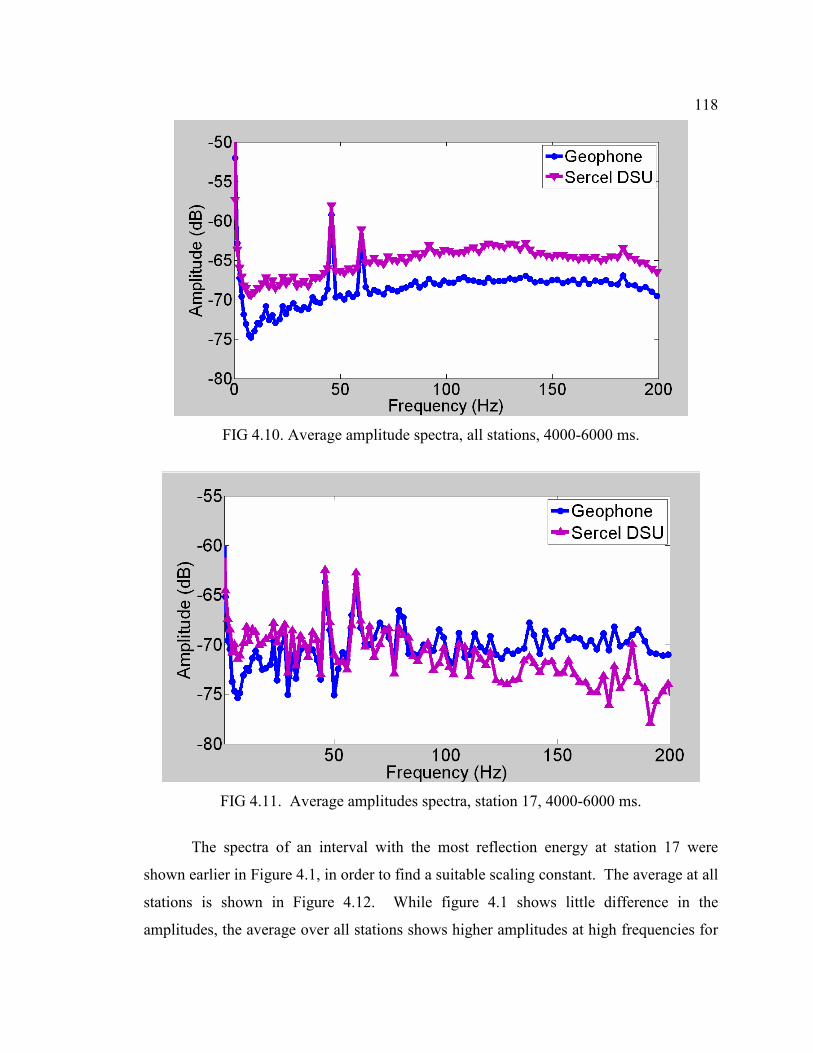
118

FIG 4.10. Average amplitude spectra, all stations, 4000-6000 ms.

FIG 4.11. Average amplitudes spectra, station 17, 4000-6000 ms.

The spectra of an interval with the most reflection energy at station 17 were

shown earlier in Figure 4.1, in order to find a suitable scaling constant. The average at all

stations is shown in Figure 4.12. While figure 4.1 shows little difference in the

amplitudes, the average over all stations shows higher amplitudes at high frequencies for

119

the DSU. This is likely to be related to the high frequency noise seen at many stations as

well, suggesting the coupling problems have slightly affected the overall data quality,

though only in amplitudes over 30 times smaller than the dominant frequencies.

FIG 4.12. Average amplitude spectra, all traces, 250-4000 ms.

iii. Phase spectra

Since the amplitudes were quite similar over the initial reflections at station 17,

this station will be used to look for differences in the acceleration-domain phase. It can

be observed that where the amplitudes are similar, the phase is also similar. This is true

at both near offset traces (Figure 4.13) and farther offsets (Figure 4.14). These

similarities were predicted in the laboratory tests, where the amplitude and phase of the

sensors was very close to their modeled response for almost all amplitudes and

frequencies.

120

FIG 4.13. Amplitude and phase spectra, station 17, trace 11.

121

FIG 4.14. Phase difference, station 17, trace 25.

The FX phase plots (Figure 4.15) few differences at station 17, as expected. At

high frequencies it is difficult to show any differences, but by looking at the low

frequencies (Figure 4.16), it appears as though the geophone is slightly more coherent

than the DSU.

122

FIG 4.15. FX phase coherence at station 17. Left: geophone. Right: DSU.

FIG 4.16. Closeup of Figure 4.13, 0-20 Hz. Left: geophone. Right: DSU.


Time domain filter panels (Figures 4.17 to 4.21) again show what is expected: the

geophone gathers are cleaner and clearer, largely due to the differences in coupling in the

field. One exception is in the low frequencies (Figure 4.18), where the DSU did not

perform well after clipping, and the near offset traces do not match well at all. Perhaps

the most notable thing is in the 35-50 Hz panel (Figure 4.20) the DSU record contains

almost as much information as the geophone record, despite the much stronger noise.

Nonetheless, in the near-offset traces of the next panel (Figure 4.21), it appears the

geophone bandwidth at this station may have been slightly larger than the DSU.

123

FIG 4.17. Filter panel (0/0/5/8), station 17. Left: geophone. Right: DSU.

FIG 4.18. Filter panel (1/2/5/8). station 17. Left: geophone. Right: DSU.


124



v. Crosscorrelation

There is no reference for the crosscorrelations here, as there was not a second

geophone present to compare with the first geophone. Figure 4.22 shows that the middle

traces of the gather are very similar in appearance. The numerical crosscorrelation values

(Figure 4.23) generally exceed 95%. Specifying an interval where reflections are most

dominant, and filtering to the dominant frequencies in the reflections, improves the

correlation somewhat (Figure 4.24). Crosscorrelations hovering around 99% over much

125

of the signal band shows that it is largely the raw data itself that results in similar

processed sections (Hauer, 2008, pers. comm.), not the procedures of the processing flow.

FIG 4.22. Comparison of acceleration traces at station 17. Blue – geophone, red – DSU.

FIG 4.23. Trace by trace crosscorrelation at station 17, entire traces.

126

FIG 4.24. Trace by trace crosscorrelation at station 17, 500-1000 ms, bandpass filtered

10/15/45/50.

4.4 Horizontal component

Station 17 is also well planted for both sensors, as shown in the horizontal

component data (Figure 4.25). The DSU was somewhat less noisy than the geophone at

station 17, but not at all stations (Figure 4.26). The noise appears generally comparable,

and the gathers appear very similar.

FIG 4.25. Acceleration receiver gather, station 17, H1 component, 0-2000 ms.

. Left: geophone. Right: DSU.

127

FIG 4.26. Acceleration receiver gather, station 18, H1 component, 0-2000 ms. Left:

geophone. Right: DSU.

i. Amplitude Spectra (global)

Unlike the Violet Grove test there is clipping in the horizontal components here,

so clipped traces do not contribute to the global spectra. The spectra for station 17 are

shown in Figure 4.27, and the same scaling constant used for the vertical component

works well for the horizontal data. The spectra match closely up to about 100 Hz. The

low frequencies match particularly well, which tended to be true of all well coupled

stations (4.28).

128

FIG 4.27. Amplitude spectra, all stations, excluding clipped traces.

FIG 4.28. Amplitude spectra, all stations, closeup of low frequencies.


Looking again at the recordings before the first breaks (Figure 4.29), we see the

geophones record significantly lower values during an interval where there should only

129

be ambient and electrical noise. The poorly planted DSU stations appear to have affected

the horizontal component data more significantly than the vertical component.

FIG 4.29. Amplitude spectra, all stations, traces 41-54, 0-250 ms.

Examining only a well-planted DSU station (Figure 4.30), we see the noise levels

are more comparable. Still the DSU recorded larger amplitudes up to 60 Hz, but then

does not have the same advantage at high frequencies because the DSU elements are not

as far below the surface as the nail-style geophone.

130

FIG 4.30. Amplitude spectra, station 17, traces 41-54, 0-250 ms.

The latest arrivals (Figure 4.31) are also noise dominated, and the average DSU

has much larger amplitudes across the spectrum than the average geophone. In a well-

planted DSU (Figure 4.32), the same pattern is seen again with the higher noise below 50

Hz. The noise floor modeling suggests this is at least 20 dB too large to be the system

noise, but the pattern’s continual reappearance suggests it is something inherent to the

sensors. Finally, excluding first breaks, (Figure 4.33), the average DSU has significantly

larger high frequencies, twice as large as in the vertical component. Though still fairly

small, they could interfere with signal processing (presuming they represent noise). Once

again, when data from a well planted station (Figure 4.34) are inspected, we see a strong

similarity between the spectra, just like the vertical component.

131

FIG 4.31. Amplitude spectra, all traces, 5000-6000 ms.

FIG 4.32. Amplitude spectra, station 17, all traces, 5000-6000 ms.

132

FIG 4.33. Average amplitude spectra, all stations, 250-5000 ms.

FIG 4.34. Amplitude spectra, station 17, all traces, 500-5000 ms.

iii. Phase spectra

These phase spectra correspond to the same interval as the amplitude spectra in

Figure 4.34. A relatively near offset trace (Figure 4.35) and far offset trace (Figure 4.36)

133

show that over the frequencies where the amplitude spectrum is similar and it is assumed

the same signals are reaching the sensors, that the phase spectra overlap. Where the

amplitudes are similar, the phase rarely separates by more than a few degrees, and never

in a consistent manner.

An estimate of the signal is again evaluated with F-X complex phase spectra

(Figure 4.37). The spectra are in general extremely similar, even down to the lowest

frequencies (Figure 4.38). The geophone appears again to be slightly more coherent at

low frequencies, but the difference is very small.

FIG 4.35. Amplitude and phase spectra, station 17, trace 9, 500-6000 ms.

134

FIG 4.36. Amplitude and phase spectra, station 17, trace 30, 500-6000 ms.

135

FIG 4.37. FX phase spectra, station 17. Left: geophone. Right: DSU.

FIG 4.38. Closeup of Figure 4.32, 0-20 Hz.

iv. Time domain filter panels

Filter panels of the horizontal component data show very much the same result as

the vertical component. The correction to acceleration domain boosts low frequencies in

the geophone record, and contributes a significant amount of very low frequency noise.

The DSU does not suffer the same problem at the very lowest frequencies (Figure 4.39).

When frequencies below 2 Hz are cut out, the filter panels become nearly

indistinguishable (4.40). Over the remainder of the frequency bands (Figures 4.41 to

4.42), there remains little difference between the sensors, just a small amplitude

difference at an event between 35 and 50 Hz (Figure 4.43).

136

FIG 4.39. Station 17, filter panel 0/0/5/8. Left, geophone. Right, DSU.

FIG 4.40. Station 17, filter panel 1/2/5/8. Left, geophone, Right, DSU.

FIG 4.41. Station 17, filter panel 5/8/30/35. Left: geophone. Right: DSU.

137

FIG 4.42. Station 17, filter panel 30/35/50/55. Left: geophone. Right: DSU.

FIG 4.43. Station 17, filter panel, 60/65/80/85. Left: geophone. Right: DSU.

v. Crosscorrelation

Where the sensors were similarly coupled to the earth, the recorded traces were

very similar (Figure 4.44). Most of the crosscorrelation values (Figure 4.45) are over

90%, with a couple nearing 99%. It is plain that the source responsible for the noise

around trace 40 on the filter panels has a much more profound effect on the horizontal

components than the vertical component. Since the noise does not appear to more

severely affect the horizontal record than the vertical record at this station, this is likely

due to S-waves traveling with very low velocity through the near surface and reaching the

geophone and DSU at significantly different times, while the same is not true of

138

refraction and reflection energy. This leads to a very different trace between the two

sensors, and is essentially highlighting the problem with intra-array statics in 3C

recording. This noise interferes strongly with the signal band, so selecting a time interval

or bandpass filter will improve the crosscorrelations somewhat in the noisy region

(Figure 4.46).

FIG 4.44. Comparison of acceleration traces, station 17. Blue – geophone, red – DSU.

FIG 4.45. Crosscorrelation between geophone and DSU, station 17, entire traces.

139

FIG 4.46. Crosscorrelation between geophone and DSU, station 17. Bandpass filter

(6/10/40/45), 500-1000 ms.

4.5 Discussion

The DSU-428 sensors at Spring Coulee suffered from many poor plants, resulting

in more noise in the average DSU than in the average geophone record, especially before

the first breaks and at late arrival times. At well-planted stations, the DSU was observed

to have larger noise amplitudes than the geophone below 60 Hz, but smaller noise

amplitudes above. Even in the interval with strong reflection energy, the noise could still

be seen to have an effect above ~75 Hz. Coupling was clearly the largest driver of data

quality in this survey. The largest amplitudes were essentially identical.

Where the sensors were similarly planted, there was no evidence of nonlinearity,

though in the time domain gathers and filter panels it was seen that the low frequencies

did not recover quickly once the DSU was driven to clip. This did not affect the general

seismic signal band. The signal interval spectra closely matched closely where the

sensors were similarly planted.

The both vertical and horizontal components had generally high crosscorrelations

when source-generated signal was isolated. As at Violet Grove, the very low frequencies

in the vertical component appeared cleaner in the geophone data, though in the horizontal

component they were cleaner in the DSU. Overall, filter panels showed there was very

little practical difference between the sensors.

140

CONCLUSIONS

This work began with a discussion of the mechanics of seismic sensors, based on

the simple harmonic oscillator model. Both traditional analog geophones and MEMS

accelerometers can be viewed as harmonic oscillators, over the range of frequencies used

in seismic exploration. Where they differ is in the transduction used to record the motion

of the proof mass. Geophones use a coil/magnet inductor, while MEMS accelerometers

use capacitors. This defines the proof mass motion that they detect. Geophones detect

the velocity of the coil relative to the magnet, and MEMS accelerometers detect the

displacement of the central proof mass in the silicon sandwich. Due to the MEMS

accelerometers’ very high resonance, any residual displacement of the proof mass is

proportional to the acceleration of the case. For timescales on the order of the desired

signal frequencies, the digital feedback loop in the MEMS accelerometer effectively acts

as an additional analog restoring force. This effectively stiffens the suspension of the

proof mass, which further increases the resonance, and increases the range of frequencies

where the ‘high-frequency resonance’ approximation is true. For the useful seismic band,

MEMS accelerometer output is a direct representation of the case, and thus ground,

acceleration. Due to weight and sensitivity requirements, the resonance of a geophone is

neither very high nor very low relative to the frequencies of the desired signal. This

means no approximation can be made, and geophone output is not a direct representation

of any domain of ground motion.

A correction based on a simple harmonic oscillator can be found to correct

geophone output to any domain of ground motion desired. The usual ‘geophone response

curve’ used to ‘dephase’ geophone data is one of these corrections. Frequency domain

corrections for one sensor will only vary from each other by some factor of iω, since iω

represents a time derivative in the frequency domain. The correction to calculate ground

acceleration from geophone data is simply the usual ‘geophone response curve’ divided

by iω. The MEMS accelerometer does not require correction because the assumption that

its resonance is much higher than the highest recorded frequency is reasonable over the

141

entire seismic band. If frequencies that were high enough to violate this assumption were

to be considered, a more detailed model for the MEMS accelerometer would have to be

considered.

Both sensors use ∆Σ loops to digitize their analog output, and in both cases it

largely defines their noise floors. Geophones maintain digitization as a separate process,

where the analog output is generated in the sensor and then sent to an external digitizer.

MEMS accelerometers, on the other hand, derive their feedback from within the

digitizing process, which keeps the proof mass centered so most nonlinearities in the

capacitors can be ignored. Some factors, such as feedback voltage and sampling rate, can

also be adjusted to help control the nonlinearities over the frequency band of interest.

The sense-feedback process inside a MEMS accelerometer is essentially a physical

analog for the electrical sense-feedback that converts geophone data from analog to

digital.

The point at which the ∆Σ loop adds the system noise provides an inherent

difference between the sensors. Accelerometers have lower noise at high frequencies; the

cross-over is estimated here at between 40 and 110 Hz, depending on the recording

systems being compared. Conversely, geophones have lower noise at frequencies below

that cross-over point (down to ~5 Hz for a 10 Hz geophone), despite their decrease in

sensitivity below resonance. As a result, geophones may have the advantage in detecting

very small signals if the dominant frequency lies between 5 and ~60 Hz, while MEMS

accelerometers may have an advantage in detecting very small high frequency signals.

This may mean MEMS accelerometers perform best at small to medium offsets and

travel times, where the high frequency signals may exist that are not detectable by a

geophone. Geophones may be best when using very long offsets or very long listening

times for deep exploration targets where even the dominant frequencies may be very

small. A direct observation of the recording system noise floor was not made in the field

data, because the ambient noise was found to be significantly larger than recording

system noise the land data presented. If we rely on fold to reduce the random ambient

noise, that brings signals above ~30 dB below the ambient noise into consideration. If

the noise floor presents a barrier to this 30 dB reduction, where the other sensor’s noise

142

floor would not, then the sensor with the lower noise floor would have a useful

bandwidth advantage. At Violet Grove, the lowest ambient noise was generally at above

~120 Hz, where the MEMS accelerometer has the noise floor advantage. Under very

windy conditions at Spring Coulee, the opposite was true (where DSUs were properly

planted).

Modeling with zero-phase and minimum-phase wavelets shows that the raw data

from the two sensors should not appear remarkably different, and accelerometer data will

not be 90-degree phase shifted from geophone data. In addition, if one wishes to recover

from a geophone Vibroseis data with the Klauder wavelet embedded as it was input to the

vibrator truck, it is necessary to use the ground displacement correction equation. Raw

accelerometer data will have the double time derivative of the input Klauder wavelet

embedded, as will geophone data after the acceleration correction has been applied.

An important point is that the concept of ground motion domain applies only

before deconvolution. No matter what the domain of the embedded wavelet was (ground

velocity, ground acceleration or geophone distorted motion), the most common

application of deconvolution is to ‘remove’ it by whitening the spectrum to come nearer

to recovering the earth’s reflectivity. Deconvolution seeks to isolate the frequency band

that is related to the reflection signal of the earth and flatten it; maximizing all

frequencies that contain desired information and minimizing those that do not. Once this

has happened, the original character of the ground motion is lost, and the seismic data can

no longer be seen as relating to a ground motion domain. They no longer represent the

motion of the ground; they represent, to some degree, the reflectivity. Modeling with a

known reflectivity series showed no advantage to using acceleration data as input to

deconvolution over geophone data. Also, no ground motion domain showed a significant

advantage over the others in terms of robustness to noise.

Lab tests from the VASTA project confirm that modern geophone elements are

manufactured to very close tolerances and all parameters estimated from the harmonic

scan tests fell within quoted variances, with one minor exception. The accelerometer

element, while not exactly the same as digital-grade seismic acquisition elements, also

performed to within fractions of a dB from its stated gain and a few degrees of the

143

expected zero phase lag. These results were for ‘moderate’ excitation levels which

started near a hundred µm/s2 at low frequencies and increased up towards a few m/s

2 at

high frequencies (100-200 Hz). This is the range of amplitudes encountered in actual

land seismic data, as the field gathers showed an ambient noise floor around 100-200

µm/s2 (about 80 dB down from 1 m/s

2).

Neither sensor followed their modeled response below signal strengths of ~0.5

µm/s2. However, this is well below 30 dB down from the ambient noise, and would not

likely be recoverable from land surface seismic data. The fact that both sensors are

observed to perform very well down to dynamic inputs of 1 µg or below is itself

remarkable.

Finally, two sets of comparison field data were examined; one from Violet Grove,

Alberta, and one from Spring Coulee, Alberta. Both sets compared Sercel’s DSU system

to analog geophones, using dynamite shots to maximize the recorded bandwidth. All

comparisons were done in the ground acceleration domain. At Violet Grove, the sensors

were very carefully planted and were largely frozen into the ground, producing generally

good coupling. The geophones were recorded with an ARAM Aries instrument, while

the DSU-408 sensors were recorded using a Sercel system. This resulted in some

differences needing to be accounted for, particularly the different anti-alias filters. The

Aries filter also used a 3 Hz lowcut, which the Sercel did not. After correcting for

instrument response, the geophone and accelerometer amplitudes were very similar down

to ~5 Hz. Also, numerical ground acceleration values calculated using the geophone

sensitivity constants did not directly match the amplitudes used by the Sercel system, and

a scaling constant was needed. Examination of gathers that included both far and near

offsets showed that the constant was applicable for all non-clipped values, which is

equivalent to stating no nonlinearity was observed in the Violet Grove data. The same

constant was equally applicable to the horizontal component data.

The data were examined in the frequency domain. Over an interval excluding the

largest amplitudes and first breaks (concentrating on reflection signal), it was shown that

the only consistent difference between the two sensors was an increase in amplitudes

below 5 Hz. In the largest amplitudes, the DSU tended to have smaller high frequency

144

content. Isolating the smallest arrivals and ambient noise, the DSU vertical component

appeared to have lower noise than geophones above 100 Hz, and higher noise below 50

Hz. The DSU horizontal component was somewhat noisier than the geophones

throughout the investigated band, in part because the horizontal sensing elements are

housed within the upper portion of the case, not below the ground surface like the vertical

sensing element. In general the clearest observation was that nail-style sensors were

shielded from high-frequency noise compared with surface-style sensors.

The data were also examined in the time domain with filter panels and

crosscorrelations between the geophone acceleration and accelerometer traces. The

crosscorrelations were very high where coupling was equivalent, and at some stations the

DSU traces were indistinguishable from the geophone traces. The filter panel tests failed

to show any significant difference at the high frequencies, but any differences may be

hidden beneath ambient noise, not visible unless further processing were undertaken. At

the very low frequencies, the DSU did not outperform the geophone in the vertical

orientation, but appears to be less noisy in the horizontal orientation. It is unclear

whether MEMS accelerometers can improve on the horizontal component low

frequencies of a geophone enough to offer valuable new information. Further study is

needed. In general, it appeared the two sensors performed according to their expected

response over a wide range of frequencies and amplitudes, confirming the lab

observations.

The data considered from Spring Coulee were a series of dynamite shots recorded

by Geospace SM-24 geophones and Sercel DSU-428 units both recorded using the Sercel

instrument. This eliminated any concerns about differences in the recording, ensuring

any differences could be traced to the receiver station. Here, however, geophones were

observed to be better planted than the DSUs. Again, one constant was applicable to the

vertical data of all amplitudes.

In vertical component data, it appears the amplitude spectra are very similar

where coupling conditions are similar. The high amplitudes were nearly identical

irrespective of coupling conditions, perhaps a sign of an improved high amplitude

response of the DSU-428 over the DSU-408. Even in cases where DSU coupling was

145

poor, the reflection data amplitudes were nonetheless fairly similar, with some additional

high frequency noise content. Time domain filter panels did not show a significant

difference in signal bandwidth. Crosscorrelations over the time interval dominated by

shot-generated signal were high (>98%), though not as high as at Violet Grove. In the

horizontal component, the data were again very similar. No large differences were

observed in the amplitude or phase spectra, beyond the difference in ambient noise

already mentioned. The DSU appears to be more coherent below 2 Hz, but no significant

differences were observed between 2 and 5 Hz in the time domain. Crosscorrelations

were generally high, especially when concentrating on a time interval and frequency band

dominated by source-related signal. Poor crosscorrelations were observed near an

external noise source, which did not have as large an effect on the vertical component,

and are likely related to the low velocity of shear waves in the near surface.

Where properly coupled, consistent differences between DSUs and geophones

were small, and it was difficult to come to any conclusion on which more accurately

recorded the ground’s motion. Both sensors can be said to have very faithfully and

similarly recorded the source-generated signals.

Future work

Much work can be done to further delineate and exploit differences between

geophones and MEMS accelerometers. In my opinion, chief among these is to determine

if richer low frequency content is recorded by the accelerometer than by common seismic

exploration geophones (10 Hz resonance). Ferguson (1996) showed a clear example of a

low-resonance (2 Hz) geophone providing better low frequencies for impedance

inversion than a standard (10 Hz) geophone. Over the 2-10 Hz range, the 10-Hz

geophone amplitude response drops by 12 dB/octave relative to a 2-Hz geophone. By

comparison, a 10-Hz geophone amplitude response drops only by 6 dB/octave relative to

an accelerometer. Whether the accelerometer provides as much additional low-frequency

information as a low-resonance geophone is not yet determined. Inspection of filter

panels in this thesis does not lead to great confidence. Ferguson (1996) showed that

146

greater low frequency content after migration, even by a few dB, was indicative of a

clearer, more conclusive inversion result. Migration and impedance inversion of a

comparison line between 10-Hz geophones and accelerometers may be able to come to a

clear conclusion. Alternately, comparison of the 2 and 10 Hz resonance raw records from

the Blackfoot broadband data used by Ferguson (1996) to the accelerometer and 10 Hz

geophone records, respectively, of a comparison line may also be useful.

In the lab, it may be useful to run the exciters with a synthetic data trace of a

smaller sinusoid overlain on a larger sinusoid. It may reveal which sensor is better at

representing two different amplitudes at the same time. If the actual motion of the

exciters can be monitored accurately enough, driving the sensors with actual field

recorded traces from both near and far offsets may more accurately reproduce field

recording, under controlled ambient conditions.

The relevance of choice of domain to processing could be an important topic. It

appears to the eye that there is little apparent difference in stacked data processed from

geophone and acceleration domains (Hauer, 2008, pers. comm.), and testing with spiking

deconvolution showed little difference as well. However, when processing flows are

tailored to suit one domain, perhaps some advantage may become evident.

The noise floors of the sensors show that there is an inherent difference between

geophones and accelerometers, and accelerometers should be less noisy at high

frequencies. In surface seismic field data, this was difficult to investigate because the

ambient noise was larger. It would be interesting to test MEMS accelerometers in a

borehole or on the seabed where the recording system noise floors may be relevant.

One more area of interest is the ability of a MEMS accelerometer to detect the DC

component. It may be that in order to achieve low noise and high linearity current

MEMS accelerometers were forced to give up some accuracy in the DC measurement.

However, it may be possible to engineer a MEMS accelerometer with the ability to

record microgravity. Then, with a package of six MEMS chips, it would be possible to

have microseismic, microgravity and tiltmeter applications in one sensor, which could be

of great value in monitoring situations.

147

REFERENCES

Barzilai, A., 2000, Improving a geophone to produce an affordable broadband seismometer:

Ph. D. thesis, Stanford University.

Bernstein, J., 2003, An overview of MEMS sensing technology: Sensors Magazine.

Brincker, R., Lago, T, Andersen, P. and Ventura, C., 2001, Improving the classical geophone

sensor element by digital correction: Proceedings: IMAC-XXIII Conference &

Exposition on Structural Dynamics.

Brown, R. J., Stewart, R. R. and Lawton, D. C., 2001, A proposed polarity standard for

multicomponent seismic data: Geophysics, 67 (4), 1028-1037.

Cambois, G., 2002, Instrumentation or how many sows’ ears does it take to make a silk purse?:

The Leading Edge, 21, 817–818.

Cary, P. W., 2001, Seismic deconvolution: Assumptions, convictions and concerns: CSEG

Recorder, 26(3), 27-28.

Cooper, N. M., 2002, Seismic Instruments: What’s new? What’s true?: CSEG Recorder, 27(12),

36-45.

Farine, M., Thorburn, N. and Mougenot, D., 2003, General application of MEMS sensors for

land seismic acquisition – is it time?: Extended abstract, CSPG Annual Meeting.

Ferguson, R. J., 1996, P-S seismic inversion: Modeling, processing, and field examples: M. Sc.

thesis, University of Calgary.

Gibson, J., Burnett, R., Ronen, S. and Watt, H., 2005, MEMS sensors: Some issues for

consideration: The Leading Edge, 24, 786-790.

Heath, B., 2005, An update on string theory, or the grand unified approach to land acquisition:

The Leading Edge, 24, 1020-1026.

Kraft, M., Lewis, C. P. and Hesketh, T. G., 1997, Control System Design Study for a

Micromachined Accelerometer: Second IFAC Workshop on New Trends in Design of

Control Systems, Smolenice.

Kraft, M., 1997, Closed loop digital accelerometer employing oversampling conversion, Ph. D.

thesis, Coventry University

Lawton, D. C., Bertram, M. B., Margrave, G. F. and Gallant, E. V., 2006, Comparisons between

data recorded by several 3-component coil geophones and a MEMS sensor at the Violet

Grove monitor seismic survey: CREWES Research Report, 18, 2.1-2.24.

Lines, L. R., and Ulrych, T. J., 1977, The old and the new in seismic deconvolution and wavelet

estimation: Geophysical Prospecting, 25, 512-540.

Lowrie, W., 1997, Fundamentals of geophysics: Cambridge University Press.

Margrave, G. F., 1999, Seismic signal band estimation by interpretation of f-x spectra:

Geophysics, 64(1), 251-260.

Maxwell, P., Tessman, J. and Reichert, B., 2001, Design through to production of a MEMS

digital accelerometer for seismic acquisition: First Break, 19(3), 141-144.

148

Mewhort, L., Bezdan, S. and Jones, M., 2002, Does it matter what kind of Vibroseis

deconvolution is used?: Extended abstract, CSEG Annual Meeting.

Mierovitch, L., 1975, Elements of vibration analysis: McGraw-Hill.

Mougenot, D., 2004, Land seismic: needs and answers: First Break, 22, 59-63.

Mougenot, D. and Thorburn, N., 2004, MEMS-based 3C accelerometers for land seismic

acquisition: Is it time? The Leading Edge, 23, 246-250.

Peterson, J., 1993, Observations and modeling of seismic background noise: Report 93-322, US

Geological Survey.

Sallas, J. J., 1984, Seismic vibrator control and the downgoing P-wave: Geophysics, 49(6), 732-

740.

Speller, K. and Yu, D., 2004, A low-noise MEMS accelerometer for unattended ground sensor

applications: Proceedings of the SPIE, 5417, 63-72.

Telford, W. M., Geldart, L. P. and Sherriff, R. E., 1977, Applied geophysics: Cambridge

University Press.

Vermeer, G., 2004, An ambitious geometry for 3D land acquisition: The Leading Edge, 23,

1043-1046.

Wielandt, E., 2002, Seismometry: Ch. 18 in IASPEI International Handbook of Earthquake and

Engineering Seismology, Academic Press.

149

Appendix A. Derivation of simple harmonic oscillator equation

The following equations (A1-A5) and the accompanying derivation are based on

Lowrie (1997) and Wielandt (2002). Sensors for seismic exploration are generally an

inertial (i.e. ‘proof’) mass (m) suspended by a spring from a frame, which is coupled to

the earth. We will use “up” as the positive direction within the sensor, and “down” as the

positive direction for the ground motion. When the earth is displaced by a seismic wave

by amount u, the frame displaces relative to the proof mass. The amount the frame

moves relative to the proof mass (i.e., the amount of stretch in the spring), is x. This is

the motion detected by the transducer, which transforms it into the electrical output. If

there is no motion of the proof mass relative to the frame, there is nothing for the sensor

to detect. Note that if an incident ground motion is upwards, the deflection of the proof

mass relative to the frame will be downward, and vice versa. A downward (positive)

earth motion produces an upward (positive) motion of the proof mass relative to the case,

and a positive peak on the seismic record. This is in accord with the SEG polarity

convention (Brown et al., 2001). The net motion (i.e., the movement of the proof mass

when viewed from outside) is n, which is equal to x+u. This is illustrated in Figure A1.

The sensor must be damped or else it would be overcome by vibrations at its

natural frequency and fail to record any other signals, which would be pushed out of its

dynamic range. Damping is represented by the dashpot in Figure A1, and can be thought

of as viscous, as if the mass was surrounded by dense fluid. In reality, damping is often

achieved electrically, such as a high resistance shunt in the case of geophones.

We will consider the free body diagram of the proof mass as the wave passes.

Newton’s 2nd

law states that the product of mass and acceleration of the proof mass will

equal the sum of the forces acting on the proof mass. At any time there are three forces

acting on the mass: the gravitational attraction of the earth, the upward force of the

spring, and the damping force of the dashpot. We can write:

dampingspringgravityproofproof FFFam ++= . (A1)

We are using the undisturbed position of the proof mass as x=0, where we can see that a

portion of the force of the spring will cancel gravity:

150

dampinglspringspringCompgravityproofproof FFFFam +++= )( Re , (A2)

where FspringComp is the amount of spring force compensating for gravity, and FspringRel is

the amount of force that is greater or lesser than the gravity compensation. Equation A2

simplifies to:

dampinglspringproofproof FFam += Re , (A3)

where FspringRel is positive when the spring applies more force than at its undisturbed

position (i.e. when x is negative), and vice versa. So equation A3 becomes:

t

xckxxu

tm proof ∂

∂−−=+−

∂

∂)(

2

2

, (A4)

because the relative spring force is always opposite in sign to x (and a positive spring

force from a negative displacement is increased by an upward ground acceleration), and

the damping force is always opposing the proof mass velocity. The spring constant is k,

and c is the coefficient of viscous damping. Now we can use the definitions ω02=k/ mproof

and c=2λk and divide through by mproof to write:

2

22

002

2

2t

ux

t

x

t

x

∂

∂=+

∂∂

+∂

∂ωλω , (A5)

where λ is the damping ratio.

Figure A1. Proof mass motion as a wave passes. Ground motion is u, proof mass motion relative to the frame is x, and the net motion is n.

151

Appendix B. MATLAB code for motion domain conversion

B1. Full service program to calculate any ground motion domain from any geophone or

accelerometer

%%This program requires a seg-y file of seismic data and the sampling interval of the

%%data. It operates trace-by-trace and no scaling is applied. If true ground motion

%%amplitudes are required in SI units, the sensitivity constant of the geophone or

%%accelerometer must be accounted for separately.

clear;

%Load seismic wiggles

disp (' Enter filename of SEG-Y file ');

sw=input (' ---> ','s');

seismic=altreadsegy(sw);

[nrows,ncolumns]=size(seismic);

%Define time vector

disp (' Enter sampling interval in ms ');

delt=input (' ---> ')*0.001;

tmin=delt;

tmax=nrows*delt;

tsw=tmin:delt:tmax;

%Define frequency vector

fnyq=0.5/delt;

fmin=fnyq/65537;

delf=fnyq/65537;

nsamples=fmin:delf:fnyq;

%Oooo... so many choices

endnow=false;

disp (' Enter 1 for geophone data, 2 for accelerometer data ')

choice=input(' --> ')

if choice == 1

disp (' Enter geophone resonant frequency ')

f0=input(' --> ')

disp (' Enter geophone damping coefficient ')

d0=input(' --> ')

disp (' Enter domain to transform into: Displacement=1, Velocity=2, Acceleration=3 ')

domain=input(' --> ')

elseif choice == 2

disp (' Enter domain to transform into: Displacement=1, Velocity=2, Geophone

equivalent=3 ')

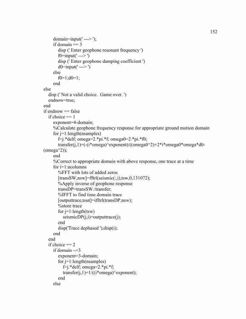
152

domain=input(' ---> ');

if domain == 3

disp (' Enter geophone resonant frequency ')

f0=input(' ---> ')

disp (' Enter geophone damping coefficient ')

d0=input(' ---> ')

else

f0=1;d0=1;

end

else

disp (' Not a valid choice. Game over. ')

endnow=true;

end

if endnow == false

if choice == 1

exponent=4-domain;

%Calculate geophone frequency response for appropriate ground motion domain

for j=1:length(nsamples)

f=j.*delf; omega=2.*pi.*f; omega0=2.*pi.*f0;

transfer(j,1)=(-(i*omega)^exponent)/((omega0^2)+2*i*omega0*omega*d0-

(omega^2));

end

%Correct to appropriate domain with above response, one trace at a time

for i=1:ncolumns

%FFT with lots of added zeros

[transSW,nsw]=fftrl(seismic(:,i),tsw,0,131072);

%Apply inverse of geophone response

transDP=transSW./transfer;

%IFFT to find time domain trace

[outputtrace,tout]=ifftrl(transDP,nsw);

%store trace

for j=1:length(tsw)

seismicDP(j,i)=outputtrace(j);

end

disp('Trace dephased ');disp(i);

end

end

if choice == 2

if domain ~=3

exponent=3-domain;


f=j.*delf; omega=2.*pi.*f;

transfer(j,1)=1/((i*omega)^exponent);

end

else

153


f=j.*delf;

omega=2.*pi.*f; omega0=2.*pi.*f0;

transfer(j,1)=(-(i*omega)^exponent)/((omega0^2)+2*i*omega0*omega*d0-

(omega^2));

end

end

%Correct to appropriate domain with above response, one trace at a time

for i=1:ncolumns

%FFT with lots of added zeros

[transSW,nsw]=fftrl(seismic(:,i),tsw,0,131072);

%Apply geophone response, or shift motion domain with frequency-domain

%integration

transDP=transSW.*transfer;

%IFFT to find time domain trace


%store trace

for j=1:length(outputtrace)

seismicDP(j,i)=outputtrace(j);

end

disp('Trace dephased ');disp(i);

end

end

end

B2. Function to correct geophone to ground acceleration

function [acceltrace,tout]=geophonetoaccel(geotrace,t,resonance,damping)

%Takes in a trace of geophone data, its time vector along with the resonance

%in Hz and damping ratio (a fraction of critical, e.g. 0.7) of the

%geophone. Returns the ground acceleration trace (accelerometer trace).

delt=t(2)-t(1);

fnyq=0.5/delt;

fmin=fnyq/65537;

delf=fnyq/65537;


for a=1:length(nsamples)

f=a.*delf; omega=2.*pi.*f; omega0=2.*pi.*resonance;

transfer(a,1)=-(i*omega)/((omega0^2)+2*i*omega0*omega*damping-(omega^2));

end

[transSW,nsw]=fftrl(geotrace,t,0,131072);

154

transDP=transSW./transfer;


for b=1:length(t)

acceltrace(b)=outputtrace(b);

end

tout=t;

B3. Function to correct acceleration records to geophone output

function [geotrace,tgeo]=acceltogeophone(acceltrace,t,resonance,damping)

%Takes in a trace of accelerometer data, its time vector along with the resonance

%in Hz and damping ratio (a fraction of critical, e.g. 0.7) of some

%geophone. Returns the trace that geophone would have acquired.

delt=t(2)-t(1);

fnyq=0.5/delt;

fmin=fnyq/65537;

delf=fnyq/65537;


for a=1:length(nsamples)

f=a.*delf; omega=2.*pi.*f; omega0=2.*pi.*resonance;

transfer(a,1)=-(i*omega)/((omega0^2)+2*i*omega0*omega*damping-(omega^2));

end

[transSW,nsw]=fftrl(acceltrace,t,0,131072);

transDP=transSW.*transfer;


for b=1:length(t)

geotrace(b)=outputtrace(b);

end

tgeo=t;

155

Appendix C. Optimal damping for accelerometers

There must be a damping value for each resonance frequency that extends the

range of flat response as much as possible in both amplitude and phase for an

accelerometer. For geophones, since resonance is within the band of measured

frequencies, lowering damping to achieve a flatter phase response will amplify any

incoming vibrations at resonance. This will take up some of the dynamic range of the

recording system, and is probably not desirable. For an accelerometer, with resonance

well beyond the desired signal band, the resonating frequency can be filtered prior to

recording so it does not take up recording dynamic range, and need not be represented

accurately, so long as it does not interfere with accurate representation of the signal band.

A lower damping value will extend the flat range in phase, but compromise the

flat range in amplitude, and vice versa. It should be possible to find an optimal damping

value that extends both flat ranges. Beginning with the amplitude and phase separated

out of the complex response (Mierovitch, 1975):

222 )2()1(

1)(

XXA

λω

+−= , (C1)

and

−

= −2

1

1

2tan)(

X

Xλωϕ , (C2)

where X=ω/ω0. Considering amplitudes (equation 37) first, it can be shown that

0))(

11()24(

2

22 =−+−+ω

λA

ZZ , (C3)

where Z=X2. Finding the solution to the quadratic gives

2

))(

11(4)24()24(

2

222

ωλλ

AZ

−−−±−−

= , (C4)

which in turn becomes

156

2

))(

11(4)24()24(

2

222

0

ωλλ

ωωA

−−−±−−

= . (C5)

This is an expression for the frequency at which the amplitude will become some given

value A. Here only damping ratios lower than 0.7 will be considered, so the value of the

amplitude will rise towards a peak at resonance as frequencies increase. Assuming a

value of A=1.025 means the result will be the frequency at which 2.5% error is

introduced into the amplitudes. This is essentially setting a 2.5% error threshold.

Proceeding for the phase separated out of the complex response (Mierovitch,

1975):

0))(tan(2))(tan( 2 =−+ ωϕλωϕ XX , (C6)

which leads to

))(tan(2

))((tan(4)2(2 22

ωϕωϕλλ +±−

=X , (C7)

and

))(tan(

))((tan( 22

0 ωϕωϕλλ

ωω+±−

= . (C8)

Now we can calculate the frequency at which the phase value exceeds some arbitrary

threshold. Setting φ=0.025π results in the same 2.5% threshold as for amplitudes. Of the

two possible frequencies resulting from equation C5, one is lower and one is higher than

resonance. This analysis is concerned only with the lower solution. Of the two possible

frequencies resulting from equation C8, one is positive and one is negative. The negative

solution is ignored. Results calculated over a range of frequencies from 1 to 2000 and a

range of damping ratios from 0.1 to 0.7 are shown in Figure C1.

157

FIG B1. Frequencies at which the error threshold is met. Blue surface is amplitude, red is

phase. The intersection of the surfaces is the highest frequency where both error

thresholds are met.

It is clear that higher damping ratios (up to 0.7) favour a flat amplitude response,

as the frequency at which the threshold is exceeded increases with higher damping.

Similarly, low damping ratios favour a flat phase response. The intersection of the

surfaces is the highest frequency where both amplitude and phase are less than 2.5%

away from their flat response value. As the resonant frequency increases, so does this

threshold frequency, so higher resonance always extends both flat responses. Most

interesting, however, is the fact that a single damping value is optimal for all resonant

frequencies. This can be explained by setting equations C5 and C8 equal to each other,

so both error requirements are met at some frequency. It is evident that the only variables

remaining are tan(φ), A and λ. As both tan(φ) and A are the arbitrary error constraints,

and are constant, an single optimal damping value for all resonance frequencies can be

expected. From Figure C1, clearly a damping ratio around 3.2 will preserve both flat

amplitude and flat phase response the widest band possible, no matter the resonant

frequency of the MEMS accelerometer.

Seismic sensing: Comparison of geophones and ...

Documents

Transcript of Seismic sensing: Comparison of geophones and ...