1

Seismic modeling of incised valley fills of the Red Fork Formation in the Anadarko Basin… A way to resolve invisible channels. Yoryenys Del Moro*, The University of Oklahoma, USA Yoscel Suarez*, Chesapeake Energy and The University of Oklahoma, USA Kurt Marfurt, The University of Oklahoma, USA. Summary The Red Fork formation consists of incised valley fills which are formed during changes of sea level. While many of the producing wells can be correlated to stratigraphic features seen in the seismic, many of them do not, giving raise to the term “invisible” channels. The main objective of this work is to identify the different lithologies present in the valley system and model their response using a modern full waveform elastic equation algorithm. Given this response we will be able to predict whether to reprocess the data for AVO analysis, acquire higher frequency and more densely sampled P-wave data, or even to acquire SH-SH data. Introduction Incised valley fills are distinctive features formed in a low-stand system tract. They are filled in a transgresive system tract. Most of the time they represent a reservoir characterization puzzle, since there are multiple sediments mixed in due to the changes of sea level. The seismic reservoir characterization of different lithologies is very challenging to image with seismic data. In this particular area the productive Red Fork sands cannot be seismically mapped, and are therefore called them invisible or “ghost” packages. The main objective of this study is to create a base seismic model in which different characteristics (geophysical and geological) will be varied in order to understand the lithological variations within the valley system, to ultimately conclude what is the best approach to resolve those invisible valley fills that the conventional 3D seismic interpretation workflow cannot achieve. Since this survey contains over 600 wells, it serves as a natural laboratory to justify more expensive acquisition and processing in neighboring less-developed acreage. Description of the data and Geological framework. The seismic surveys used in this study were acquired by Amoco during three different stages from 1993 until 1996 to be finally merged into a 136 mi2 survey, which is located in the eastern part of the Anadarko basin (Figure 1). The

dominant frequency of the seismic data ranges from 50 Hz up to 80 Hz. Seismic attribute assisted interpretation and well data were used to correlate the valley fills events. Correlation between seismic and well data has been partially achieved by using different seismic attributes, and with this we were able to recognize the study target zone.

Figure 1: Location map of surveys realized in the Anadarko Basin in Oklahoma- USA. All of them are showing the year in which they were done. (Taken and modified from Peyton, et al. 1998). The Red Fork zone is characterized by three coarsening upward marine parasequences (Lower, Middle, and Upper Red Fork, divided according to the oil and gas content in each one Red Fork sands are characterized by their sorting which enhances their reservoir quality. According to Tolson et al. (1993) the entire interval has some “breaks” or shale layers; all of which are produced by varying changes of sea level during the time of the Cherokee deposition (Desmoinesian) in the large Enid embayment from the Pennsylvanian age. The lower Red Fork is mainly deep-marine shale and siltstone. The middle is marine dominated and was deposited into a relatively deep basin on a steep, unstable delta-front slope and finally the upper Red Fork deposited in shallower water (in which we are going to focus to

Seismic modeling of incised valley fills of the Red Fork.

2

realize this study) is a deltaic sequence more fluvial dominated. The Red Fork overlays regionally extensive limestone intervals which are the Inola Lime and Novi lime and it is superposed by the Pink Lime, that is characterized by containing fish scales, coffee-ground to branch-size lignitic plant debris, and brackish to shallow-marine ostracodes, linguloid brachiopods, Tasmanites algae, and gastropods. The incised valley fills of the Red Fork Formation are originated by multiples stages of fill and incision, resulting in a stratigraphically complex internal architecture (Peyton, 1998). In this way five different phases or stages of fill were defined by previous authors that had worked on with this data set. Withrow et al. (1968) in his research defined four distinct phases of sand deposition, one during which channel sand was deposited, two phases of offshore-bar deposition and a last one in which the sea retrograded and allowed channel sand to be deposited. What is defined as a Phase II sandstone was interpreted as a body that had been deposited as subaqueous offshoresand bars and it contains a layer of shale which is indicative of low wave energy. Phase III is distinguished by an increase of sea level and sand grains are thinner in this section. In Phase IV, sandstones seemed to have been deposited in transgressions in which older sediments had been eroded. This last phase appears to be deposited in stream and river channels, then the sea level rised and in this moment is when the carbonates ( Pink lime) was formed. Peyton et al. (1998) defined those four phases and added a fith one (Figure 3). Phase I is chartacterized by being the earliest valley event, for that reason, in many places it had been eroded. It consists on rocks usually poorly correlative shales, silts and tight sandstones superposing a basal “lag” deposit. Phase II was deposied in a period of valley widening and maturation, also showin a finner grain size. Phase III was deposited during a transgression sequence which brought marine shales. Phase IV is described to be a interbeded of sand and shales with and addition of coaly shale close to the base of this phase. Phase IV differs between the definition of Withrow and Suarez, this last one explains that the facies of this stage of fill are deposited in a lagoon/coal swamp or by a head of a delta environment. In logs is evident the high response to the coal shale presence. For the last phase identified, we see the correlation between both definition, wherein a raise of sea level in this time

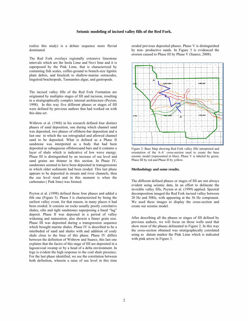
eroded previous deposited phases. Phase V is distinguished by non- productive sands. In Figure 3 is evidenced the erosion caused to Phase III by Phase V (Suarez, 2008).

Figure 2: Base Map showing Red Fork valley fills interpreted and orientation of the A-A’ cross-section used to create the base seismic model (represented in blue). Phase V is labeled by green, Phase III by red and Phase II by yellow.

Methodology and some results. The different defined phases or stages of fill are not always evident using seismic data, In an effort to delineate the invisible valley fills, Peyton et al. (1999) applied. Spectral decomposition imaged the Red Fork incised valley between 20 Hz and 50Hz, with appearing at the 36 Hz component. We used these images to display the cross-section and create our seismic model. After describing all the phases or stages of fill defined by previous authors, we will focus on those wells used that show most of the phases delineated in Figure 2. In this way the cross-section obtained was stratigraphically correlated using as datum marker the Pink Lime which is indicated with pink arrow in Figure 3.

Seismic modeling of incised valley fills of the Red Fork.

3

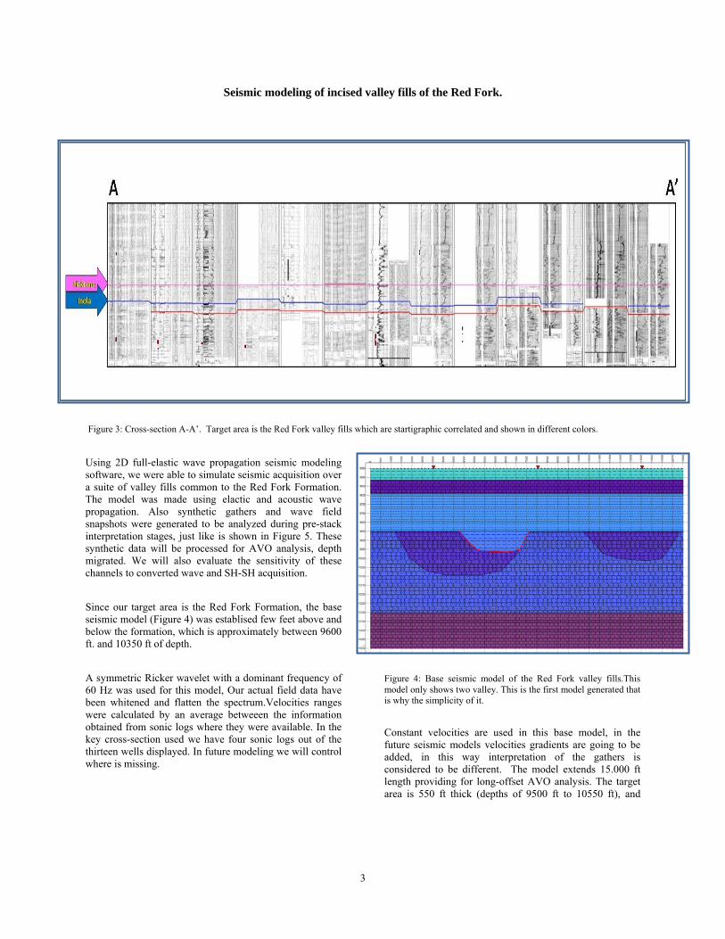
Figure 3: Cross-section A-A’. Target area is the Red Fork valley fills which are startigraphic correlated and shown in different colors.

Using 2D full-elastic wave propagation seismic modeling software, we were able to simulate seismic acquisition over a suite of valley fills common to the Red Fork Formation. The model was made using elactic and acoustic wave propagation. Also synthetic gathers and wave field snapshots were generated to be analyzed during pre-stack interpretation stages, just like is shown in Figure 5. These synthetic data will be processed for AVO analysis, depth migrated. We will also evaluate the sensitivity of these channels to converted wave and SH-SH acquisition. Since our target area is the Red Fork Formation, the base seismic model (Figure 4) was establised few feet above and below the formation, which is approximately between 9600 ft. and 10350 ft of depth. A symmetric Ricker wavelet with a dominant frequency of 60 Hz was used for this model, Our actual field data have been whitened and flatten the spectrum.Velocities ranges were calculated by an average betweeen the information obtained from sonic logs where they were available. In the key cross-section used we have four sonic logs out of the thirteen wells displayed. In future modeling we will control where is missing.

Figure 4: Base seismic model of the Red Fork valley fills.This model only shows two valley. This is the first model generated that is why the simplicity of it.

Constant velocities are used in this base model, in the future seismic models velocities gradients are going to be added, in this way interpretation of the gathers is considered to be different. The model extends 15.000 ft length providing for long-offset AVO analysis. The target area is 550 ft thick (depths of 9500 ft to 10550 ft), and

Seismic modeling of incised valley fills of the Red Fork.

4

consists of 5 layers of varying thickness. In one of the layers two valley fills are included with the thickest one being 350 ft and the other about 150 ft. In future models more details will be added inside of the valley fills to prove if we could resolve the different phases of fill. The vertical resolution of this seismic model is calculated by λ/4, where λ is the wavelenght and is 164.04 ft. Vertical resolution is 41 ft, so we will be able to resolve those valley fills set on the model. Compared to the real seismic data in which the velocity is 14.200 ft/s, same dominant frequency of 60 Hz, the vertical resolution is 59 ft. This shows that the seismic parameters used in real seismic could be utized in order to resolve the valley fills created in this seismic model.

Figure 5: Shot gather (left) and wavefront propagation model (right) Conclusions and Ideas for future work The selection of the parameters in the modeling generation is critical since is going to affect all the results. For instance, variation of seismic parameters is very significant since those are going to define the resolution limits of our seismic data. For future work will be generate two models differing by a numerical factor in density, to later subtract both of them and see the result. An example of this methodology will be the creation of a sand-filled vs. a shale filled valley fills model, in order to study their response in full-stack to later do the AVO analysis. Through pre-stack depth migration we will able to determine which parameters are affecting the lateral resolution of the seismic data to be able to visualize incised valley fills.

Acknowledgments Special thanks to Mark Falk of Chesapeake for all his patience correlating wells and for all of those who contributed with their important and appreciable ideas. Thanks to Chesapeake management for allowing us to use their well and seismic data for this effort. Finally, thanks to Tesseral for use of their wave-equation modeling software in this model study.