Seismic facies classification away from well control - The role of augmented training data using basin modeling to improve machine learning methods in exploration.

Per Avseth (Dig Science) and Tapan Mukerji (Stanford University)

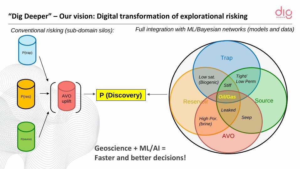
“Dig Deeper” – Our vision: Digital transformation of explorational risking

P(res)

P(trap)

P(source)

Reservoir

Trap

Source

AVO

AVOuplift

Low sat.(Biogenic)

High Por.(brine)

Seep

Tight/Low Perm

Stiff

Leaked

Oil/Gas

Full integration with ML/Bayesian networks (models and data)Conventional risking (sub-domain silos):

P (Discovery)

Geoscience + ML/AI = Faster and better decisions!

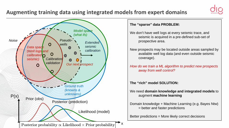
Augmenting training data using integrated models from expert domains

Ground truth (knowns & unknowns)

Noise

Data space(Well logs and calibrated seismic)

Our next prospect

Extended seismic calibration

Likelihood (model)

Prior (obs)Posterior (prediction)

Model space(what ifs)

Calibration/validation

The “sparse” data PROBLEM:

We don’t have well logs at every seismic trace, and seismic is acquired in a pre-defined sub-set of prospective area.

New prospects may be located outside areas sampled by available well log data (and even outside seismic coverage).

How do we train a ML algorithm to predict new prospects away from well control?

The “rich” model SOLUTION:

We need domain knowledge and integrated models to augment machine learning

Domain knowledge + Machine Learning (e.g. Bayes Ntw) = better and faster predictions

Better predictions = More likely correct decisions

Pseudo-wells

P(x)

x

QSI with augmented training data

Augmented Training dataProbability Density Functions (PDFs)

Inverted Elastic Properties

Lithofacies Mapsand Uncertainty

Bayesian Machine Learning

Well-LogsGeology

Statistical Rock

Physics

Seismic Inversion

Seismic Data

Scenario testing based on geological expertise

4

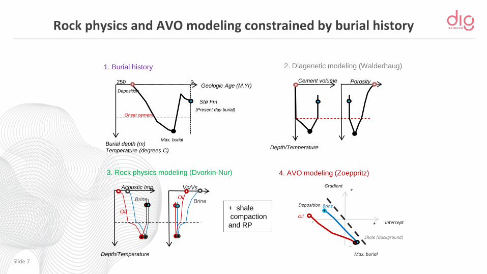
AVO classification constrained by burial history in Loppa High Area, Barents Sea

Case Example 1:

(The Leading Edge, 2003)

AVO classification constrained by rock physics depth trends

We need to dig deeper!

Extend technology by adding more G&G domain input/constraints:

1) Include diagenesis2) Include tectonics (burial, uplift,

erosion)3) Honor sequence stratigraphic

principles

Once upon a time…

Vp/VsAcoustic Imp.

PorosityCement volume

Rock physics and AVO modeling constrained by burial history

Slide 7

1. Burial history

Burial depth (m)Temperature (degrees C)

Geologic Age (M.Yr)0250

Stø Fm

Deposition

Max. burial

(Present day burial)

2. Diagenetic modeling (Walderhaug)

Depth/Temperature

Onset cement

3. Rock physics modeling (Dvorkin-Nur)

Depth/Temperature

Oil

Brine OilBrine

4. AVO modeling (Zoeppritz)

+ shalecompactionand RP Intercept+-

+

-

Gradient

Deposition Brine

Oil

Shale (Background)

Max. burial

Burial constrained AVO modeling to create syntethic training dataUnconsolidated sand example: Oil-filled sand = AVO class III

“Frying pan”

Brine

Oil

Brine

Oil

OilBrine

Shale

Shale

Brinesand

Burial curve

70 C

Fluid trend

Compaction trend

AVO constrained by burial

Burial constrained AVO modeling to create syntethic training dataCemented sandstone example: Oil-filled sst = AVO class IIp

“Frying pan”

Brine sst

Oil

Brine sst

OilFluid trend

Compaction trend

OilBrine

Shale

Shale

Brinesand

Burial curve

70 C

AVO constrained by burial

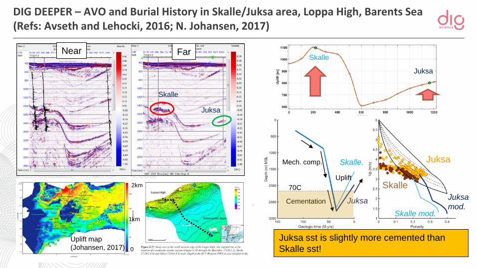
DIG DEEPER – AVO and Burial History in Skalle/Juksa area, Loppa High, Barents Sea(Refs: Avseth and Lehocki, 2016; N. Johansen, 2017)

Juksa

Skalle

Skalle.

Juksamod.

Skalle mod.Juksa

70C

Cementation

Mech. comp.

Uplift

Juksa sst is slightly more cemented than Skalle sst!

Skalle

Juksa

Skalle

Juksa

Uplift map(Johansen, 2017)

2km

1km

0

Near Far

Generating AVO training data for Skalle well (7120/2-3S)

Vp Vs Rho3.2 1.73 2.31

10% 10% 5%

1 0.8 0.6

0.8 1 0.8

0.6 0.8 1

Vp Vs Rho3.3 1.6 2.42

5% 5% 5%

1 0.8 0.6

0.8 1 0.8

0.6 0.8 1

Vp Vs Rho3.0 1.5 2.5

5% 5% 5%

1 0.95 0.8

0.95 1 0.8

0.8 0.8 1

mean

std

Cov.

Brine properties:

AVO classification constrained by burial history at Skalle well

Most likely brine saturated sandstones predicted at Juksa well

-log(γ)

GasOil

BrineHeterol.Shale

Skalle Juksa

Simulation of AVO training data from burial trends at Juksa well (7120/6-3S)

Vp Vs Rho3.4 2.0 2.3

10% 10% 5%

1 0.8 0.6

0.8 1 0.8

0.6 0.8 1

Vp Vs Rho3.5 1.9 2.45

5% 5% 5%

1 0.8 0.6

0.8 1 0.8

0.6 0.8 1

Vp Vs Rho3.0 1.45 2.54

5% 5% 5%

1 0.95 0.8

0.95 1 0.8

0.8 0.8 1

mean

std

Cov.

AVO facies/fluid classification constrained by burial history at Juksa well

Most likely oil saturated sandstones predicted at Juksa well

-log(γ)

GasOil

BrineHeterol.Shale

Skalle Juksa

Inputs for nonstationary PDF-s

Stationary pdfs

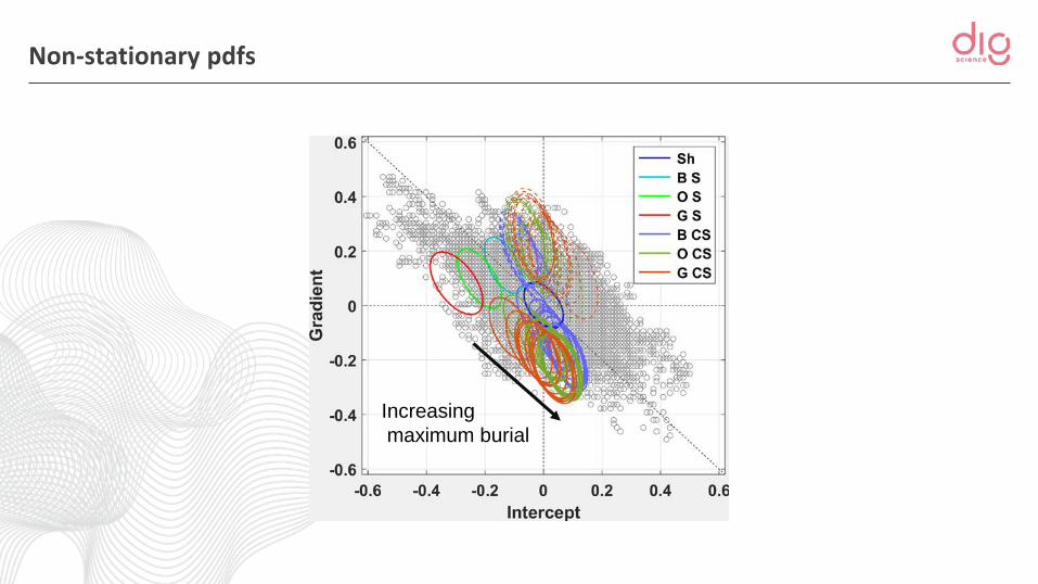
Non-stationary pdfs

Increasingmaximum burial

Stationary

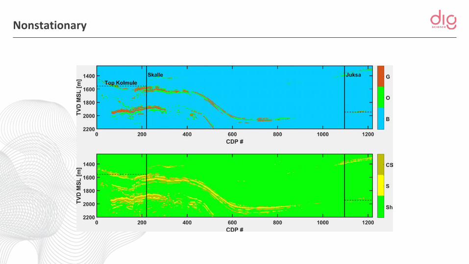
Nonstationary

Integrating statistical rock physics and pressure and thermal historymodeling to map reservoir lithofacies in the deepwater Gulf of Mexico(Wisam, Mukerji, Sheirer and Graham, Geophysics, July-Aug. 2018)

Case Example 2:

Basin Modeling (BPSM in one slide)

Honoring the geology and solving for the physics in geologic timeModeling pressure and thermal history and rock properties

+

Stratigraphy

+

Rock Properties

Coupled PDEs in time and spaceSimulation

Predicted Rock PropertiesModel Outputs

Calibration

Geologic Inputs

Structure

Basin and Petroleum System Modeling - BPSM

Comparative Study of QSI ScenariosValue of extrapolating pseudo logs at Well A2 other wells (C and D) held out for validation

Actual Well A Data

Actual Well B Data

Basin Modeling-Rock Physics

Extrapolation at Well A

ReferenceScenario 1Scenario 2

salt

salt

Well B Well A

Reservoir

22

Middle Miocene deep water sand reservoirsNW Well B Well A SE

10 km0

Thunder Horse North Field Thunder Horse Field

Basin Modeling Outputs

2D basin model across Thunder Horse structureSpatial trends in effective stress and temperature conditions

A

B

23

Spatial Trend of PDFs

Scenario 1: PDFs from well B aloneScenario 2: series of interpolated PDFs; Predicted spatial variations of Vp, Vs and density from basin modeling and rock physics

sandstone

shale

Distance (km)

Vp(m

/s)

Bayesian classificationDetermination of most likely lithofacies and probabilities of lithofacies

Reference Case

Sandstone

Shale

0 2 km

Scenario 1 Scenario 2

Results: Improved sandstone thickness and volume predict

Scenario 1: underestimates net volume by 23%Scenario 2: net volume difference of 0.5% only

Scenario 1 – Reference Ave. thickness error ~ 200 m

Scenario 2 – Reference Ave. thickness error ~ 25 m

Error (m) Error (m)25

Dept

h (m

)

GR Pr(Sand) Pr(Sand) Pr(Sand)

Well C

Validation wellReference

Workflow 11 well alone

Workflow 21 well + BPSM & RP

0 1 0 1 0 1

25

G&G integrated with ML/AI (summary)• Domain knowledge (Sedimentology, Basin Modeling, Rock Physics/QI)

augments Machine Learning!

• Many sources of uncertainty:- geological scenario- geological heterogeneity- imperfect and incomplete data, - approximate rock physics models,

• Need for multiple “possible” Earth models (scenarios)

• Need for Uncertainty Quantification.

• Remember we are often looking for rare events!

Key take aways

• Machine learning not a “black box” – We need G&G domain experts!

• Phase transition in massive computations and machine learning is an opportunity!

• How do we take advantage of this transition in our research and business?

Geosciences & Machine Learning

If we can meet the challenges,If we can avoid the pitfalls,We can benefit from the opportunities

Just dig it!

Acknowledgements

• Thanks to Dig Science colleagues (Kristin Dale, Tore Nordtømme Hansen, Kristian Angard, Carine Zeier, Reidar Muller).

• Thanks to Ivan Lehocki for key contributions

• Thanks to Lundin-Norway for collaboration/input to Skalle and Juksa discoveries (Article in The Leading Edge, 2016).

• Thanks to TGS Nopec for seismic data used in this study.