
seismic design and evaluation of multistory buildings using - Ideals
172
SEISMIC DESIGN AND EVALUATION OF MULTISTORY BUILDINGS USING YIELD POINT SPECTRA Mid-America Earthquake Center prepared by: Edgar F. Black and Mark Aschheim Civil and Environmental Engineering University of Illinois at Urbana-Champaign Urbana, Ilinois July, 2000
Transcript of seismic design and evaluation of multistory buildings using - Ideals
SEISMIC DESIGN AND EVALUATION OFMULTISTORY BUILDINGS USING YIELD
POINT SPECTRA
Mid-America Earthquake Center
prepared by:
Edgar F. Blackand
Mark Aschheim
Civil and Environmental EngineeringUniversity of Illinois at Urbana-Champaign
Urbana, Ilinois
July, 2000
ii
ABSTRACT
SEISMIC DESIGN AND EVALUATION OF MULTISTORY BUILDINGSUSING YIELD POINT SPECTRA
Constant ductility response spectra are presented for 15 recorded earthquakes ground
motions using the Yield Point Spectra (YPS) representation. Yield Point Spectra are used for
analysis and design of SDOF structures. The spectra were computed for bilinear and stiffness
degrading load-deformation models, for displacement ductilities equal to 1, 2, 4 and 8.
A methodology for the performance-based seismic design of regular multistory
buildings using Yield Point Spectra is described. The methodology is formulated to make use
of current code approaches as much as possible while allowing the design engineer to limit
the peak displacement response and, to some extent, the peak interstory drift to user-specified
values. To achieve this objective, the design methodology makes use of an equivalent SDOF
model of the building.
A method to estimate peak displacement response and interstory drift indices of
multistory buildings using YPS and establish SDOF formulations is also presented. The
method may be considered a new nonlinear static procedure (NSP). Interstory drift indices
(IDIs) are estimated using deformed shapes of the building based on the first mode shape and
combinations of the first and second mode shapes.

iii
ACKNOWLEDGMENTS
This report was prepared as a doctoral dissertation by the first author in partial
fulfillment of the requirements for the Ph.D. degree in Civil and Environmental Engineering
at the University of Illinois, Urbana. The research was supervised by the second author.
This research was partially supported by the Mid-America Earthquake Center under
National Science Foundation Grant EEC-9701785.
The authors would like to thank Professors William J. Hall, Douglas A. Foutch and
Daniel P. Abrams for their helpful comments and suggestions.
Appreciation is expressed to the faculty and staff of the Department of Civil
Engineering of University of Illinois ar Urbana-Champaign for their support.
Special gratitude is expressed to Professors Timothy D. Stark, Sharon Wood, and
Neil M. Hawkins, as well as to the Department of Civil and Environmental Engineering of
the University of Illinois for the support provided.

iv
TABLE OF CONTENTS
CHAPTER 1INTRODUCTION.....................................................................................................................1
1.1 Statement of the Problem................................................................................................11.2 Historical Perspective......................................................................................................2
1.2.1 Evolution of Design Philosophies...........................................................................31.2.1.1 Life Safety.......................................................................................................31.2.1.2 Performance-Based Seismic Design................................................................4
1.3 Objectives and Scope......................................................................................................41.3.1 Objectives................................................................................................................41.3.2 Scope and Limitations.............................................................................................4
1.4 Organization....................................................................................................................5
CHAPTER 2YIELD POINT SPECTRA REPRESENTING SDOF RESPONSE.........................................6
2.1 Introduction.....................................................................................................................62.2 Description of Yield Point Spectra Representation.........................................................62.3 Application of Yield Point Spectra...............................................................................10
2.3.1 Analysis Application: Estimation of Peak Displacement......................................112.3.2 Design Application: Control of Peak Displacement and Ductility Demands.......112.3.2 Application to Performance-Based Design...........................................................15
2.4 Yield Point Spectra and Design Procedures..................................................................162.4.1 Conventional Design Procedures..........................................................................162.4.2 Yield Displacement as Key Parameter For Design...............................................17
2.5 Strength Demands and Strength-Reduction (R) Factors...............................................192.6 Numerical Examples.....................................................................................................21
2.6.1 Example 1. Accuracy of YPS Estimates...............................................................212.6.2 Example 2. Admissible Design Regions for Performance-Based Design.............22
2.7 Sample Yield Point Spectra..........................................................................................282.7.1 Ground Motions.....................................................................................................282.7.2 Selected Load-Deformation Models......................................................................33
2.8 Summary.......................................................................................................................34
CHAPTER 3EQUIVALENT SDOF MODEL OF MULTISTORY BUILDINGS......................................35
3.1 Introduction...................................................................................................................353.2 Equivalent Single-Degree-of-Freedom Modeling Technique.......................................35
3.2.1 Displacement of Equivalent SDOF From MDOF Equation of Motion................363.2.2 Yield Strength of the Equivalent SDOF System...................................................383.2.3 Displacement of the MDOF System......................................................................393.2.4 Yield Strength of MDOF System..........................................................................39
3.3 Application of the Equivalent SDOF Technique in Analysis and Design....................413.3.1 Selecting the Appropriate Deformed Shape Function {φ}....................................41
3.4 Summary.......................................................................................................................43

v
CHAPTER 4DESIGN METHODOLOGY USING YIELD POINT SPECTRA.........................................44
4.1 Introduction...................................................................................................................444.2 Design Philosophy........................................................................................................45
4.2.1 Design Premises....................................................................................................454.2.2 Yield Displacement as Fundamental Parameter for Seismic Design....................464.2.3 Control of Peak Displacement...............................................................................464.2.4 Control of Interstory Drift Index as Final Design Objective.................................474.2.5 Mixed Linear and Nonlinear Procedure................................................................47
4.3 Limitations....................................................................................................................474.4 Description of the YPS Design Methodology...............................................................484.5 Nonlinear Analysis for Verification Purposes..............................................................504.6 Design Examples...........................................................................................................51
4.6.1 Case Study 1: Design of Two 4-Story Buildings..................................................514.6.1.1 Description of the 4-Story Moment-Resistant Frames..................................514.6.1.2 Design of Flexible-4 Using the YPS for the Lucerne Ground Motion..........534.6.1.3 Design of Rigid-4 Using the YPS for the Newhall Ground Motion..............58
4.6.2 Case Study 2: Design of Two 12-Story Buildings................................................634.6.2.1 Description of the 12-Story Moment-Resistant Frames................................634.6.2.2 Design of Flexible-12 Using the YPS for the SCT1 Ground Motion............654.6.2.3 Design of Rigid-12 Using the YPS for the Takatori-kisu Ground Motion ...70
4.7 Analysis of Results........................................................................................................764.7.1 Roof Displacement Control...................................................................................764.7.2 Interstory Drift Control..........................................................................................774.7.3 Yield Displacement Stability.................................................................................774.7.4 Required Strength..................................................................................................78
4.8 Summary.......................................................................................................................79
CHAPTER 5ANALYSIS OF BUILDING PERFORMANCE USING YIELD POINT SPECTRA...........80
5.1 Introduction...................................................................................................................805.2 Nonlinear Static Procedures..........................................................................................81
5.2.1 Nonlinear Static Analysis......................................................................................815.2.1.1 Selecting the Appropriate Deformed Shape {φ}...........................................82
5.2.2 Displacement Coefficient Method.........................................................................835.2.3 Capacity Spectrum Method...................................................................................84
5.3 Conceptual Development of the YPSA Method...........................................................855.3.1 Estimating Peak Displacement Using the YPSA Method.....................................855.3.2 Estimating Interstory Drift Index Using the YPSA Method.................................86
5.4 Peak Roof Displacement and IDI Estimates for 4- and 12-Story Frames.....................875.4.1 Characteristics of Frames......................................................................................885.4.2 Peak Displacement Estimates................................................................................94
5.4.2.1 Numerical Results..........................................................................................965.4.2.2 Analysis of Results......................................................................................107
5.4.3 Estimates of Interstory Drift Indices...................................................................108

vi
5.4.3.1 Numerical Results........................................................................................1115.4.3.2 Analysis of Results......................................................................................126
5.5 The Flexible-12 Frame and the LP89CORR.090 Record...........................................1305.6 Summary.....................................................................................................................134
CHAPTER 6SUMMARY AND CONCLUSIONS....................................................................................135
6.1 Summary and Conclusions..........................................................................................1356.2 Suggestions for Future Research.................................................................................139
APPENDIX ASELECTED GROUND MOTIONS......................................................................................140
APPENDIX BC++ PROGRAM FOR DISPLACEMENT COEFFICIENT METHOD ESTIMATES........156
APPENDIX CC++ PROGRAM FOR CAPACITY SPECTRUM METHOD ESTIMATES.......................159
APPENDIX DYIELD POINT SPECTRA USED FOR PEAK DISPLACEMENT AND IDI ESTIMATES...................................................................................................................163
APPENDIX ELIST OF THE INPUT FILES USED FOR ANALYSIS OF THE FRAMES DESIGNEDWITH THE YPS METHODOLOGY....................................................................................194
LIST OF REFERENCES.......................................................................................................207

vii
LIST OF TABLES
Table 2.1 Solution Set for Life-Safe Performance Level........................................................25Table 2.2 Ground Motions Used for the Yield Point Spectra of Figures 2.18 to 2.20............32Table 3.1 Participation Factors and Effective Modal Mass Coefficients as a Function of
Number of Stories....................................................................................................42Table 4.1 Story Heights and Weights of 4-Story Buildings....................................................52Table 4.2 Design Lateral Forces and Story Shears for the Flexible-4 Frame..........................55Table 4.3 Linear Estimates for the Flexible-4 Frame..............................................................56Table 4.4 Interstory Drift Indices from Nonlinear Dynamic Analysis of the Flexible-4........58Table 4.5 Design Lateral Forces and Story Shears for the Rigid-4 Frame..............................59Table 4.6 Linear Estimates for the Rigid-4 Frame..................................................................61Table 4.7 Interstory Drift Indices from Nonlinear Dynamic Analysis of the Rigid-4.............62Table 4.8 Height and Weight of 12-Story Buildings...............................................................63Table 4.9 Design Lateral Forces and Story Shears for the Flexible-12 Frame .......................66Table 4.10 Linear Estimates for the Flexible-12 Frame..........................................................68Table 4.11 Interstory Drift Indices from Nonlinear Dynamic Analysis of the Flexible-12... .70Table 4.12 Deign Lateral Forces and Story Shears for the Rigid-12 Frame............................72Table 4.13 Linear Estimates for the Rigid-12 Frame..............................................................72Table 4.14 Interstory Drift Indices from Nonlinear Dynamic Analysis of the Rigid-12.........75Table 4.15 Peak Roof Displacement Comparison...................................................................76Table 4.16 Peak Interstory Drift Index Comparison................................................................77Table 4.17 Ratios of Yield Displacement to Building Height.................................................78Table 4.18 Comparison of Required to Actual Strength and First Period of Vibration .........78Table 5.1 First and Second Mode Shapes and Modal Interstory Drift Indices of the Flexible-4 and Rigid-4 Frames...............................................................................................................88Table 5.2 First and Second Mode Shapes and Modal Interstory Drift Indices of the
Flexible-12 and Rigid-12 Frames...........................................................................88Table 5.3 Participation Factors and Modal Mass Coefficients of the Frames........................91Table 5.4 Yield Strength and Yield Displacement of the Frames..........................................94Table 5.5 YPSA Peak Roof Displacement Estimates for Flexible-4 ...................................103Table 5.6 YPSA Peak Roof Displacement Estimates for Rigid-4........................................103Table 5.7 YPSA Peak Roof Displacement Estimates for Flexible-12..................................104Table 5.8 YPSA Peak Roof Displacement Estimates for Rigid-12......................................104Table 5.9 DCM and CSM Peak Roof Displacement Estimates for Flexible-4.....................105Table 5.10 DCM and CSM Peak Roof Displacement Estimates for Rigid-4........................105Table 5.11 DCM and CSM Peak Roof Displacement Estimates for Flexible-12..................106Table 5.12 DCM and CSM Peak Roof Displacement Estimates for Rigid-12......................106Table 5.13 Results for All Cases............................................................................................107Table 5.14 Results for NonLinear Cases...............................................................................108Table 5.15 Second Mode Peak Roof Displacement Estimates for Flexible-4.......................124Table 5.16 Second Mode Peak Roof Displacement Estimates for Rigid-4...........................125Table 5.17 Second Mode Peak Roof Displacement Estimates for Flexible-12.....................125Table 5.18 Second Mode Peak Roof Displacement Estimates for Rigid-12.........................126

viii
Table 5.19 Ratio of Absolute Peak IDI Estimates to Peak IDI Computed in NonlinearDynamic Analysis................................................................................................126
Table 5.20 Statistics of Story Ratios of Estimated IDI to Computed IDIfor 4-Story Frames...............................................................................................127
Table 5.21 Statistics of Story Ratios of Estimated IDI to Computed IDI for12-Story Frames...................................................................................................128
Table 5.22 Peak Roof Displacement for Flexible-12.............................................................130Table D.1 Equivalent SDOF Yield Strength Coefficients, Yield Displacements, and
Periods of the Frames..........................................................................................163

ix
LIST OF FIGURES
Figure 2.1 Yield Point Spectra...................................................................................................8Figure 2.2 Bilinear Load-Deformation Model...........................................................................8Figure 2.3 Relationship Between Yield Strength Coefficient (Cy) and Displacement
Ductility (�)..............................................................................................................9Figure 2.4 Using YPS to Estimate Peak Displacement...........................................................12Figure 2.5 Curve Defining Strength and Stiffness Combination to Limit uu to 8 cm.............13Figure 2.6 Admissible Design Region (Unshaded) for uu ≤ 8 cm...........................................14Figure 2.7 Admissible Design Region (Unshaded) for � ≤ 4..................................................14Figure 2.8 Admissible Design Region (Unshaded) for � ≤ 4 and uu ≤ 8 cm...........................15Figure 2.9 Seismic Performance Design Objective Matrix.....................................................16Figure 2.10 Push-over Analysis of 4-Story 3-Bay Building....................................................18Figure 2.11 Common Trends Identified in Yield Point Spectra..............................................20Figure 2.12 Estimating Ductility and Peak Displacement from YPS......................................22Figure 2.13 Time History to Compare Accuracy.....................................................................23Figure 2.14 Admissible Design Region for Operational Performance Level..........................24Figure 2.15 Admissible Design Region for Life-Safe Performance Level..............................25Figure 2.16 Admissible Design Region for Performance Objectives......................................26Figure 2.17 Time History For Numerical Example 2..............................................................27Figure 2.18 Yield Point Spectra for Short Duration Ground Motions.....................................29Figure 2.19 Yield Point Spectra for Long Duration Ground Motions.....................................30Figure 2.20 Yield Point Spectra for Forward Directive Ground Motions...............................31Figure 2.21 Load-Deformation Relationship Used to Construct Yield Point Spectra.............34Figure 3.1 Triangular and Parabolic Deformed Shapes...........................................................42Figure 4.1 Geometry of 4-Story Buildings..............................................................................52Figure 4.2 Required Yield Strength Coefficient for the Flexible-4 Frame..............................54Figure 4.3 Flexible-4 Frame....................................................................................................55Figure 4.4 Nonlinear Static Analysis of the Flexible-4 Frame................................................57Figure 4.5 Roof Displacement from Nonlinear Dynamic Analysis of the Flexible-4 Frame..57Figure 4.6 Required Yield Strength Coefficient for the Rigid-4 Frame..................................59Figure 4.7 Rigid-4 Frame.........................................................................................................60Figure 4.8 Nonlinear Static Analysis of the Rigid-4 Frame....................................................61Figure 4.9 Roof Displacement from Nonlinear Dynamic Analysis of the Rigid-4 Frame......62Figure 4.10 Geometry of 12-Story Buildings..........................................................................64Figure 4.11 Required Yield Strength Coefficient for the Flexible-12 Frame..........................65Figure 4.12 Flexible-12 Frame................................................................................................67Figure 4.13 Nonlinear Static Analysis of the Flexible-12 Frame............................................69Figure 4.14 Roof Displ. from Nonlinear Dynamic Analysis of the Flexible-12 Frame..........69Figure 4.15 Required Yield Strength Coefficient for the Rigid-12 Frame..............................71Figure 4.16 Rigid-12 Frame.....................................................................................................73Figure 4.17 Nonlinear Static Analysis of the Rigid-12 Frame................................................74Figure 4.18 Roof Displacement from Nonlinear Dynamic Analysis of the Rigid-12 Frame. .75Figure 5.1 Mode Shapes and Profiles of Modal IDI for the 4-Story Frames..........................89Figure 5.2 Mode Shapes and Profiles of Modal IDI for the 12-Story Frames........................90

x
Figure 5.3 First and Second Mode Load-Deformation Curves for the Flexible-4 Frame......92Figure 5.4 First and Second Mode Load-Deformation Curves for the Rigid-4......................92Figure 5.5 First and Second Mode Load-Deformation Curves for the Flexible-12................93Figure 5.6 First and Second Mode Load-Deformation Curves for the Rigid-12....................93Figure 5.7 Yield Points for the 4-Story Frames......................................................................95Figure 5.8 Peak Roof Displacement Comparisons for the Flexible-4 Frame.........................98Figure 5.9 Peak Roof Displacement Comparisons for the Rigid-4 Frame.............................99Figure 5.10 Peak Roof Displacement Comparison for the Flexible-12 Frame......................100Figure 5.11 Peak Roof Displacement Comparison for the Rigid-12 Frame..........................101Figure 5.12 Second Mode Yield Point for the Flexible-4 Frame..........................................110Figure 5.13 IDI Profile and Ratios Comparison for the Flexible-4 Frame............................112Figure 5.14 IDI Profile and Ratios Comparison for the Flexible-4 Frame............................113Figure 5.15 IDI Profile and Ratios Comparison for the Flexible-4 Frame............................114Figure 5.16 IDI Profile and Ratios Comparison for the Rigid-4 Frame................................115Figure 5.17 IDI Profile and Ratios Comparison for the Rigid-4 Frame................................116Figure 5.18 IDI Profile and Ratios Comparison for the Rigid-4 Frame................................117Figure 5.19 IDI Profile and Ratios Comparison for the Flexible-12 Frame..........................118Figure 5.20 IDI Profile and Ratios Comparison for the Flexible-12 Frame..........................119Figure 5.21 IDI Profile and Ratios Comparison for the Flexible-12 Frame..........................120Figure 5.22 IDI Profile and Ratios Comparison for the Rigid-12 Frame..............................121Figure 5.23 IDI Profile and Ratios Comparison for the Rigid-12 Frame..............................122Figure 5.24 IDI Profile and Ratios Comparison for the Rigid-12 Frame..............................123Figure 5.25 5% Damped Yield Point Spectra for Loma Prieta at Corralitos.........................131Figure 5.26 2.8% Damped Yield Point Spectra for Loma Prieta at Corralitos .....................132Figure 5.27 Plastic Hinges Formed During Response to the Corralitos Record...................133Figure A.1 Characteristics of the WN87MWLN.090 Ground Motion..................................141Figure A.2 Characteristics of the BB92CIVC.360 Ground Motion......................................142Figure A.3 Characteristics of the SP88GUKA.360 Ground Motion.....................................143Figure A.4 Characteristics of the LP89CORR.090 Ground Motion......................................144Figure A.5 Characteristics of the NR94CENT.360 Ground Motion.....................................145Figure A.6 Characteristics of the CH85LLEO.010 Ground Motion.....................................146Figure A.7 Characteristics of the CH85VALP.070 Ground Motion.....................................147Figure A.8 Characteristics of the IV40ELCN.180 Ground Motion.......................................148Figure A.9 Characteristics of the LN92JOSH.360 Ground Motion......................................149Figure A.10 Characteristics of the MX85SCT1.270 Ground Motion...................................150Figure A.11 Characteristics of the LN92LUCN.250 Ground Motion...................................151Figure A.12 Characteristics of the LP89SARA.360 Ground Motion....................................152Figure A.13 Characteristics of the NR94NWHL.360 Ground Motion..................................153Figure A.14 Characteristics of the NR94SYLH.090 Ground Motion...................................154Figure A.15 Characteristics of the KO95TTRI.360 Ground Motion.....................................155Figure D.1 YPS For WN87MWLN.090 and Yield Points for the 4-Story Frames ..............164Figure D.2 YPS For BB92CIVC.360 and Yield Points for the 4-Story Frames...................165Figure D.3 YPS For SP88GUKA.360 and Yield Points for the 4-Story Frames..................166Figure D.4 YPS For LP89CORR.090 and Yield Points for the 4-Story Frames...................167Figure D.5 YPS For NR94CENT.360 and Yield Points for the 4-Story Frames..................168

xi
Figure D.6 YPS For CH85LLEO.010 and Yield Points for the 4-Story Frames...................169Figure D.7 YPS For CH85VALP.070 and Yield Points for the 4-Story Frames..................170Figure D.8 YPS For IV40ELCN.180 and Yield Points for the 4-Story Frames....................171Figure D.9 YPS For LN92JOSH.360 and Yield Points for the 4-Story Frames...................172Figure D.10 YPS For MX85SCT1.270 and Yield Points for the 4-Story Frames.................173Figure D.11 YPS For LN92LUCN.250 and Yield Points for the 4-Story Frames................174Figure D.12 YPS For LP89SARA.360 and Yield Points for the 4-Story Frames.................175Figure D.13 YPS For NR94NWHL.360 and Yield Points for the 4-Story Frames...............176Figure D.14 YPS For NR94SYLH.090 and Yield Points for the 4-Story Frames................177Figure D.15 YPS For KO95TTRI.360 and Yield Points for the 4-Story Frames..................178Figure D.16 YPS For WN87MWLN.090 and Yield Points for the 12-Story Frames...........179Figure D.17 YPS For BB92CIVC.360 and Yield Points for the 12-Story Frames...............180Figure D.18 YPS For SP88GUKA.360 and Yield Points for the 12-Story Frames..............181Figure D.19 YPS For LP89CORR.090 and Yield Points for the 12-Story Frames...............182Figure D.20 YPS For NR94CENT.360 and Yield Points for the 12-Story Frames..............183Figure D.21 YPS For CH85LLEO.010 and Yield Points for the 12-Story Frames...............184Figure D.22 YPS For CH85VALP.070 and Yield Points for the 12-Story Frames..............185Figure D.23 YPS For IV40ELCN.180 and Yield Points for the 12-Story Frames................186Figure D.24 YPS For LN92JOSH.360 and Yield Points for the 12-Story Frames...............187Figure D.25 YPS For MX85SCT1.270 and Yield Points for the 12-Story Frames...............188Figure D.26 YPS For LN92LUCN.250 and Yield Points for the 12-Story Frames..............189Figure D.27 YPS For LP89SARA.360 and Yield Points for the 12-Story Frames...............190Figure D.28 YPS For NR94NWHL.360 and Yield Points for the 12-Story Frames.............191Figure D.29 YPS For NR94SYLH.090 and Yield Points for the 12-Story Frames..............192Figure D.30 YPS For KO95TTRI.360 and Yield Points for the 12-Story Frames................193

1
CHAPTER 1
INTRODUCTION
1.1 Statement of the Problem
For many years the primary objective of most earthquake structural design provisions,
such as the Uniform Building Code (International Conference of Building Officials, 1997),
has been to safeguard against major structural failures and loss of life. Others objectives such
as maintaining function, limiting damage or providing for easy repair were not explicitly
addressed in these provisions.
One major development in seismic design during the last 10 years has been increased
emphasis worldwide in performance-based seismic design, as a result of damage and
economic losses in the Loma Prieta (1989), Northridge (1994) and Hyogo-Ken Nambu
(1995) earthquakes.
Recent provisions require, in addition to the traditional life safety objective, "to
increase the expected performance of structures having a substantial public hazard due to
occupancy or use as compared to ordinary structures, and to improve the capability of
essential structures to function during and after the design earthquake" (FEMA-302/303,
1998).
The seismic performance of buildings is generally associated with structural and
nonstructural damage due to ground motions. For example, in the FEMA-273 and the Vision
2000 (SEAOC-1995) documents, performance is expressed in terms of an anticipated
limiting level of damage, termed a performance level, for a given intensity of ground motion
(Hamburger, 1997).
The importance of drift control is revealed when it is accepted that interstory drift
constitutes an acceptable measure of damage. Provisions such as FEMA-302/303 recognize
that drift control is needed to restrict damage to partitions, shaft and stairs enclosures, glass,
and other nonstructural elements.
However building codes still use strength as the main parameter and have placed the
computation of forces as the centerpiece of earthquake-resistant design, relegating drift
calculations to the end of the design process. No realistic quantification of the nonlinear

2
displacement response of the structure during the design earthquake is done, nor of the
associated structural and nonstructural damage that is likely to occur (Lepage, 1997).
In this work a new representation of earthquake spectra is introduced, known as Yield
Point Spectra (YPS). The construction of Yield Point Spectra and their application to analysis
and design of SDOF systems is discussed. It is shown that YPS can be used to reliably
determine combinations of lateral strength and stiffness that are effective to limit drift and
displacement ductility demands to arbitrary values such as those required to achieve a desired
performance. Yield Point Spectra can also be used to estimate the peak displacement and the
displacement ductility demands of structures responding to a given earthquake.
The use of the equivalent Single Degree of Freedom (SDOF) analogy plays a central
role in the procedures that are presented for using YPS in the design and approximate
analysis of multistory buildings.
For design, YPS are used to obtain the minimum lateral strength required to limit
peak roof displacement to arbitrary values for a design earthquake. Contrary to current design
methods, the proposed design methodology uses an estimate of the yield displacement of the
building rather than its fundamental period at the start of the design process. For analysis,
YPS are used to establish the peak roof displacement of a building during response to a
ground motion. Techniques to estimate interstory drift more accurately than conventional
approaches are also discussed.
The design and analysis methodologies introduced here are applied only to four case
study examples. However, it is expected that these methodologies may be generally used to
design buildings that meet current prescribed limits for interstory drift, and to meet the
performance limits that are currently being defined by the profession for use in future
performance-based seismic design codes and guidelines.
1.2 Historical Perspective
One of the major and most challenging objectives in modern structural analysis has
been to predict the response of structures (buildings) subjected to the action of earthquakes.
Considerable effort has been made in the last 30 to 40 years to try to understand the main
parameters influencing the response of structures under ground motions, and to understand

3
the main characteristics of the ground motion itself. Current recommendations and code
provisions for seismic design are based largely on work done during the last several decades.
1.2.1 Evolution of Design Philosophies
1.2.1.1 Life Safety
The objective to design structures to respond in a predictable way under different
types of earthquake excitation that the structure may experience during its life is not new.
The 1967 commentary of the Structural Engineers Association of California (SEAOC) Blue
Book introduced a general philosophy for the design of earthquake resistant buildings other
than essential and hazardous facilities. This philosophy identifies three design objectives:
(1) Prevent nonstructural damage in minor earthquake ground shaking which
may occur frequently during the service life of the structure;
(2) Prevent structural damage and minimize nonstructural damage during
moderate earthquakes ground shaking which may occasionally occur; and
(3) Avoid collapse or serious damage during severe earthquake ground shaking
which may rarely occur.
This earthquake-resistant design philosophy is also contained in the ATC 3-06 (1978)
document; however, this document focuses on life safety in the event of a severe earthquake
as "the paramount consideration in design of buildings." In practice, design for life safety has
and continues to be the main focus of routine design
Given the relatively small amount of life lost in U.S. earthquakes, existing design
procedures may be considered to be successful. However, the extent of damage to structures,
the cost of repair, and economic consequences to the areas affected by the Loma Prieta
(1989), Northridge (1994) and Hyogo-Ken Nambu (1995) earthquakes, have lead to a
broadening of the design philosophy towards what is now known as Performance-Based
Seismic Design.

4
1.2.1.2 Performance-Based Seismic Design
In this new philosophy, attention is focused on explicitly controlling the performance
of a structure over varied intensities of ground motions. Although the concepts associated
with performance-based seismic design are still in development, one criteria to control the
performance of a structure is limiting its level of damage. The perspective adopted in this
study is that damage in structures can be reduced by limiting peak roof displacement (as a
mean to indirectly limit interstory drift) and system displacement ductility to specified
values.
1.3 Objectives and Scope
1.3.1 Objectives
This study has three main objectives:
1) To explore the utility of a new representation of constant ductility response
spectra, named Yield Point Spectra, for the analysis and design of single-
degree-of-freedom systems.
2) To outline and validate a methodology for the seismic design of regular
multistory buildings using Yield Point Spectra in conjunction with establish
equivalent SDOF formulations.
3) To use Yield Point Spectra and established equivalent SDOF formulations to
develop improved estimates of peak displacement and interstory drift indices
of regular multistory buildings responding to earthquake ground motions.
The goodness of the YPS design and analysis methodologies is assessed with respect
to the results obtained from nonlinear dynamic analyses and by using the simplified analysis
methods known as the Displacement Coefficient Method and the Capacity Spectrum Method.
Comparisons are made for four case study example frames consisting of two 4-story and two
12-story moment-resistant steel frames.
1.3.2 Scope and Limitations
The proposed Yield Point Spectra methods are intended for the seismic analysis and
5
design of regular low and medium-rise frame buildings. The displacement response of all
structural elements is assumed to be dominated by flexural deformations and influenced by
seismic motions in the plane of the frame. Effects of torsional behavior and vertical ground
motions effects are not addressed.
The design methodology is restricted to obtain and distribute the strength (base shear)
required for a building to limit its peak displacement response to a prescribed value.
Established methods are relied upon for proportioning members sizes and strength; these
methods are not cover in this study.
1.4 Organization
Chapter 2 introduces Yield Point Spectra (YPS) and describes their main
characteristic, use, and potential applications. Yield Point Spectra for 15 ground motion
records and two load-deformation models are shown. An example describing the use of YPS
for the performance-based seismic design of a SDOF structure is included.
Chapter 3 presents a formulation that extends the use of Yield Point Spectra to the
analysis and design of buildings. The formulation relies on conventional equivalent single-
degree-of freedom models used to represent the response of multistory buildings.
Chapter 4 introduces a methodology for the design of regular multistory buildings.
The methodology is intended to directly limit the roof displacement and maximum interstory
drift index to user-selected values. The methodology relies on Yield Point Spectra to account
for nonlinear behavior of the multistory system.
An analysis method to estimate the peak displacement of multistory systems using
Yield Point Spectra is introduced in Chapter 5. The method is a new Nonlinear Static
Procedure (NSP). Peak roof displacement estimates obtained with the proposed method and
also with other procedures are shown and compared. The analysis method is also used to
obtain interstory drift using one deformed shape and combinations of two deformed shapes.
Finally, a special case in which the second mode causes significant yielding in one of the
frames was identified and discussed.
The summary and conclusions are presented in Chapter 6 along with
recommendations for future research.

6
CHAPTER 2
YIELD POINT SPECTRA REPRESENTING SDOF RESPONSE
2.1 Introduction
Traditional seismic response spectra plots the maximum response (displacement,
velocity, acceleration or any other quantity of interest) to a specific ground motion as
function of the system's natural period or frequency of vibration. Seismic response spectra
can be classified as elastic and inelastic response spectra. Constant ductility response spectra
(CDRS) belong to the inelastic response spectra class. CDRS plot a strength-related
coefficient corresponding to a constant displacement ductility (µ) as a function of period or
frequency.
The Yield Point Spectra (YPS) representation is a CDRS in which the strength-related
coefficient is defined as the ratio of the yield strength of the system to its weight, denoted the
yield strength coefficient (Cy) throughout this work. Contrary to other CDRS, in the YPS
representation the constant ductility curves are formed by plotting the yield strength
coefficient as a function of the system's yield displacement. Therefore, each point within one
of the curves, denoted yield point, corresponds to the yield displacement and strength
required by a SDOF oscillator to have the displacement ductility represented by the curve.
This chapter illustrates the main characteristics of YPS and their application to
analysis and design of SDOF systems. Subsequent chapters develop procedures to use YPS
for the analysis and design of multistory systems.
A set of YPS were computed for representing different earthquake motions and load-
deformation models. These were generated using PCNSPEC (Boroschek, 1991), a modified
version of NONSPEC (Mahin and Lin, 1983), and are presented at the end of this chapter in
Figure 2.18 to Figure 2.20.
2.2 Description of Yield Point Spectra Representation
Yield Point Spectra are graphs plotting curves corresponding to constant
displacement ductility demand for a specific excitation, such as the caused by an earthquake.
They represent the response of a SDOF system in terms directly useful in the design,
7
evaluation, and rehabilitation of structures for seismic loading. These graphs are directly used
for design and analysis of SDOF structures. For design, Yield Point Spectra may be used to
determine combinations of strength and stiffness sufficient to limit drift and/or displacement
ductility demands to prescribed values. For analysis, when the period and strength of a SDOF
structure are known, YPS may be used to estimate the structure's displacement ductility
demands and, therefore, its ultimate displacement. In general, these graphs help to understand
the seismic demands imposed on SDOF systems.
Since Yield Point Spectra represent the response of SDOF oscillators, having a
specific load-deformation curve and viscous damping ratio, to an individual earthquake,
different earthquakes, load-deformation models (bilinear, stiffness degrading etc.), and/or
damping ratios result in different YPS.
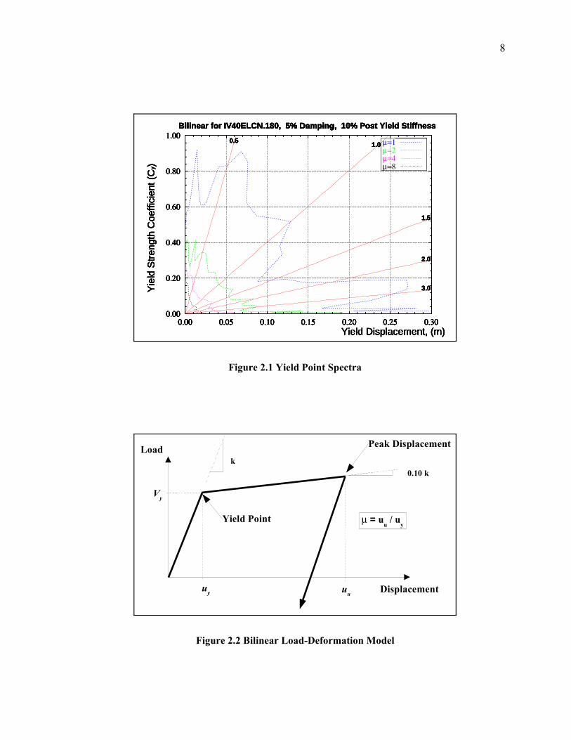
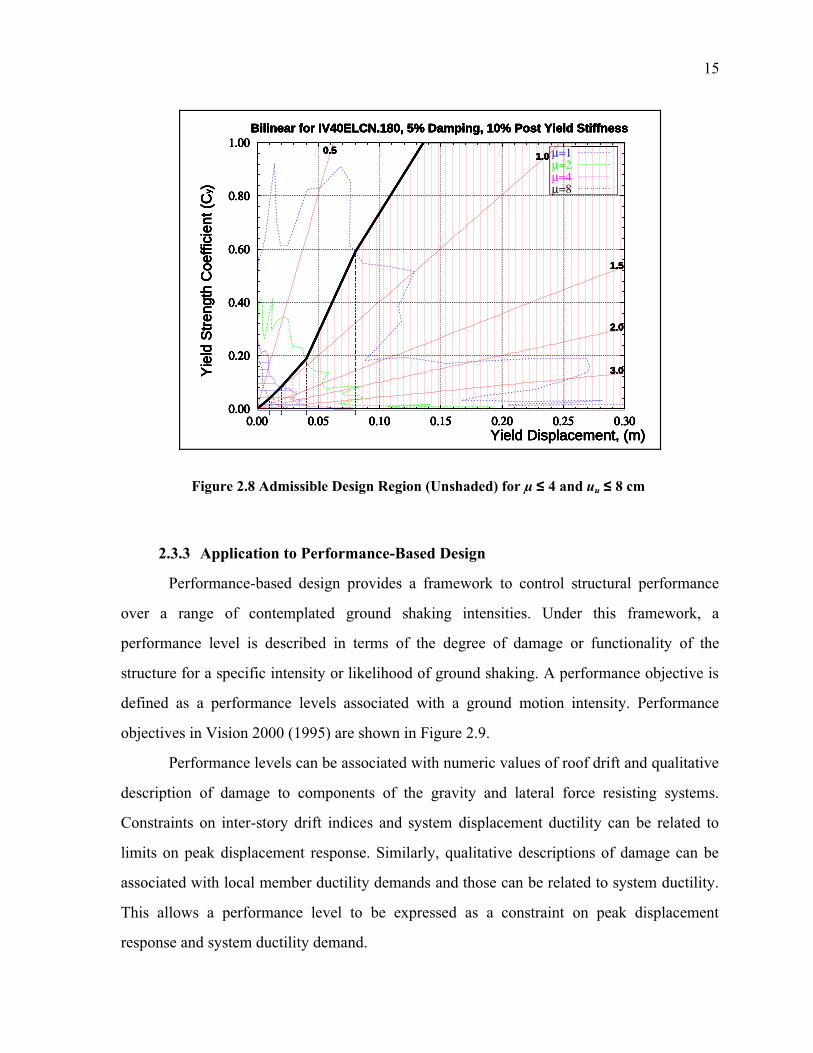
Figure 2.1 shows Yield Point Spectra for oscillators having a bilinear load-
deformation curve, shown in Figure 2.2, subjected to the 1940 record at El Centro. Viscous
damping was equal to 5% of critical damping and the post yield stiffness was 10% of the
initial elastic stiffness.
Curves representing constant displacement ductility of 1 (elastic), 2, 4, and 8 are
shown. Each point along any of the curves represents an oscillator having the yield
displacement and strength required to respond with the indicated ductility. For Figure 2.1,
each curve was generated for 45 initial periods, from 0.05 to 10.0 sec. In the format used on
that figure, lines representing initial periods radiate from the origin. Initial period of 0.5, 1.0,
1.5, 2.0, and 3.0 seconds are explicitly identified on Figure 2.1. The range of periods,
displacement ductilities, and the load-deformation model were chosen arbitrarily.
Yield Point Spectra are able to represent elastic and inelastic response of SDOF
systems. Any system having a yield point (yield displacement and strength) that lies beyond
the curve representing constant displacement ductility equal to one will respond elastically.
On the other hand, if the yield point of the system lies below the curve of constant
displacement ductility equal to one its response will be inelastic.
8
Figure 2.1 Yield Point Spectra
0.00
0.20
0.40
0.60
0.80
1.00
0.00 0.05 0.10 0.15 0.20 0.25 0.30
Bilinear for IV40ELCN.180, 5% Damping, 10% Post Yield Stiffness
Yie
ld S
tren
gth
Coe
ffici
ent (
C )y
Yield Displacement, (m)
0.51.0
1.5
2.0
3.0
µ=1µ=2µ=4µ=8
0.00
0.20
0.40
0.60
0.80
1.00
0.00 0.05 0.10 0.15 0.20 0.25 0.30
Bilinear for IV40ELCN.180, 5% Damping, 10% Post Yield Stiffness
Yie
ld S
tren
gth
Coe
ffici
ent (
C )y
Yield Displacement, (m)
0.51.0
1.5
2.0
3.0
0.00
0.20
0.40
0.60
0.80
1.00
0.00 0.05 0.10 0.15 0.20 0.25 0.30
Bilinear for IV40ELCN.180, 5% Damping, 10% Post Yield Stiffness
Yie
ld S
tren
gth
Coe
ffici
ent (
C )y
Yield Displacement, (m)
0.51.0
1.5
2.0
3.0
0.00
0.20
0.40
0.60
0.80
1.00
0.00 0.05 0.10 0.15 0.20 0.25 0.30
Bilinear for IV40ELCN.180, 5% Damping, 10% Post Yield Stiffness
Yie
ld S
tren
gth
Coe
ffici
ent (
C )y
Yield Displacement, (m)
0.51.0
1.5
2.0
3.0
0.00
0.20
0.40
0.60
0.80
1.00
0.00 0.05 0.10 0.15 0.20 0.25 0.30
Bilinear for IV40ELCN.180, 5% Damping, 10% Post Yield Stiffness
Yie
ld S
tren
gth
Coe
ffici
ent (
C )y
Yield Displacement, (m)
0.51.0
1.5
2.0
3.0
0.00
0.20
0.40
0.60
0.80
1.00
0.00 0.05 0.10 0.15 0.20 0.25 0.30
Bilinear for IV40ELCN.180, 5% Damping, 10% Post Yield Stiffness
Yie
ld S
tren
gth
Coe
ffici
ent (
C )y
Yield Displacement, (m)
0.51.0
1.5
2.0
3.0
Figure 2.2 Bilinear Load-Deformation Model
k0.10 k
uy Displacement
Load
Vy
Yield Point
Peak Displacement
uu
µ = uu / u
y

9
It is important here to point out that although smaller values for the yield strength
coefficient generally imply largest values for the displacement ductility, it is known the
relationship between these two parameters is not monotonic. For those cases when more than
one value of the yield strength coefficient results in the specified displacement ductility, the
procedure implemented in PCNSPEC (the computer program used to generate the constant
ductility curves) identifies and reports the largest yield strength coefficient, as illustrated
schematically in Figure 2.3.
The principal axes used to plot YPS are similar to those used in the Capacity
Spectrum Method (Freeman, 1978) in the sense that both use the abscissa to represent
displacement and the ordinate to represent strength. Nevertheless, the information differs
because in the Capacity Spectrum Method the displacement and the strength correspond to an
ultimate state, while in the YPS displacement and strength correspond to yield.
Simple manipulations of fundamental relations provide some useful expressions for
use with YPS. The yield strength coefficient (Cy), the yield strength (Vy ) and the initial
period of the oscillator are defined as:
Figure 2.3 Relationship Between Yield Strength Coefficient (Cy) andDisplacement Ductility (µ)
Cy
µ
Value Used For YPS
10
(2.1)
(2.2)
(2.3)
where:Cy is the yield strength coefficient,W is the oscillator weight,m is the oscillator mass,Vy is the base shear strength,uy is the yield displacement,k is the initial stiffness,T is the initial period, andg is the acceleration of gravity.
2.3 Application of Yield Point Spectra
Considerable economic losses resulting from structural damage in the Loma Prieta
(1989), Northridge (1994), and Hyogo-Ken Nambu (1995) earthquakes have focused
attention explicitly on design to control the performance of a structure over varied intensities
of ground shaking, in what is now known as performance-based seismic design.
Under this design philosophy, it is necessary for engineers to be able to accurately
estimate the peak displacement of structures responding to strong ground motions.
Additionally, it would be very desirable to have tools and procedures to determinate the
structural properties necessary to limit peak displacement response and/or displacement
ductility demands of buildings to prescribed values.
Yield Point Spectra can be applied to perform both of these operations. For the first
one, or analysis application, YPS are use to obtain accurate estimates of peak displacement
response of SDOF systems. For the second one, or design application, YPS are used to
determine the structural properties required to control peak displacement and displacement
ductility demands to specified limits. The ability to perform both operations, analysis and
design, make YPS particularly amenable to performance-based design.
V y = C y⋅W = C y⋅m⋅g
T = 2⋅π⋅mk
= 2⋅π⋅m uy
V y
= 2⋅π⋅uy
C y⋅g
C y =4⋅π2⋅uy
T 2⋅g

11
2.3.1 Analysis Application: Estimation of Peak Displacement
Several procedures to estimate peak displacement have been promoted recently and
are beginning to be used by the engineering community. Among the procedures, known as
Nonlinear Static Procedures (NSPs) in the NEHRP Guidelines for the Seismic Rehabilitation
of Buildings (FEMA-273/274; 1997), there are two methods for estimating peak
displacement response under the action of seismic loads: the Displacement Coefficient
Method and the Capacity Spectrum Method1. These methods determine displacement
estimates based on elastic response quantities, and their use require a number of steps,
approximations and assumptions. The precision of these methods has been subject of recent
discussion (Chopra et al., 1999; Aschheim et al., 1998; and Tsopelas et al., 1997).
Contrary to the two NSPs mentioned above, Yield Point Spectra contain data directly
based on inelastic response of SDOF oscillators, allowing them to provide good accuracy for
estimating the peak displacement response of SDOF systems. Their use is direct;
assumptions as the "equal displacement rule" are needed.
To illustrate how YPS are used to estimate peak displacement, consider an oscillator
having a bilinear load-deformation relationship with post-yield stiffness equal to 10% of the
initial stiffness, as shown in Figure 2.2. Assume a yield displacement of about 2.0 cm. (0.02
m), an initial period of 0.5 seconds, and viscous damping equal to 5% of critical damping.
This yield point plots right over the curve representing a displacement ductility of 2 in Figure
2.4. The resulting peak displacement for this oscillator will, therefore, be equal to twice its
yield displacement, as indicated in the figure. This ability to directly obtain peak
displacement from known yield points is a valuable feature of the YPS.
2.3.2 Design Application: Control of Peak Displacement and Ductility Demands
The Displacement Coefficient Method and the Capacity Spectrum Method are
intended for estimating the peak displacement response of existing structures. They do not
readily lend themselves to the reverse operation: determining the strength and stiffness
required for a structure in order to limit its peak displacement or its displacement ductility to
a specified value.
1 The Displacement Coefficient Method and the Capacity Spectrum Method are described in Chapter 5.

12
Yield Point Spectra, on the other hand, can be used, not only as a analysis tool to
estimate peak displacement (Figure 2.4), but also as a design tool to determine combinations
of strength and stiffness needed to limit the peak displacement and ductility demands
responses to user-prescribed values.
Figure 2.5 shows a curve defining approximate combinations of strength and yield
displacement required to limit peak displacement response to 8 cm. This curve has two parts,
representing elastic and inelastic response. The part of the curve representing inelastic
response (for µ >1) is constructed through a family of yield points. Each yield point within
the family has the property that the product of its yield displacement and its ductility demand
equals the limit displacement of 8 cm. The curve is approximate between yield points;
greater precision can be had by plotting additional constant ductility curves. The part of the
curve representing elastic response (points beyond the constant ductility curve equal to one)
is defined by the period (radial line) of an oscillator having a yield displacement equal to the
limit displacement (8 cm.). Any oscillator having a yield point that lies in the elastic part of
the curve will have a peak displacement equal to the limit displacement regardless of its
strength.
Figure 2.4 Using YPS to Estimate Peak Displacement
0.00
0.20
0.40
0.60
0.80
1.00
0.00 0.05 0.10 0.15 0.20 0.25 0.30
Bilinear for IV40ELCN.180, 5% Damping, 10% Post Yield Stiffness
Yie
ld S
tren
gth
Coe
ffici
ent (
C )y
Yield Displacement, (m)uy uu
0.51.0
1.5
2.0
3.0
µ=1µ=2µ=4µ=8
0.00
0.20
0.40
0.60
0.80
1.00
0.00 0.05 0.10 0.15 0.20 0.25 0.30
Bilinear for IV40ELCN.180, 5% Damping, 10% Post Yield Stiffness
Yie
ld S
tren
gth
Coe
ffici
ent (
C )y
Yield Displacement, (m)uy uu
0.51.0
1.5
2.0
3.0
0.00
0.20
0.40
0.60
0.80
1.00
0.00 0.05 0.10 0.15 0.20 0.25 0.30
Bilinear for IV40ELCN.180, 5% Damping, 10% Post Yield Stiffness
Yie
ld S
tren
gth
Coe
ffici
ent (
C )y
Yield Displacement, (m)uy uu
0.51.0
1.5
2.0
3.0
0.00
0.20
0.40
0.60
0.80
1.00
0.00 0.05 0.10 0.15 0.20 0.25 0.30
Bilinear for IV40ELCN.180, 5% Damping, 10% Post Yield Stiffness
Yie
ld S
tren
gth
Coe
ffici
ent (
C )y
Yield Displacement, (m)uy uu
0.51.0
1.5
2.0
3.0
0.00
0.20
0.40
0.60
0.80
1.00
0.00 0.05 0.10 0.15 0.20 0.25 0.30
Bilinear for IV40ELCN.180, 5% Damping, 10% Post Yield Stiffness
Yie
ld S
tren
gth
Coe
ffici
ent (
C )y
Yield Displacement, (m)uy uu
0.51.0
1.5
2.0
3.0
0.00
0.20
0.40
0.60
0.80
1.00
0.00 0.05 0.10 0.15 0.20 0.25 0.30
Bilinear for IV40ELCN.180, 5% Damping, 10% Post Yield Stiffness
Yie
ld S
tren
gth
Coe
ffici
ent (
C )y
Yield Displacement, (m)uy uu
0.51.0
1.5
2.0
3.0

13
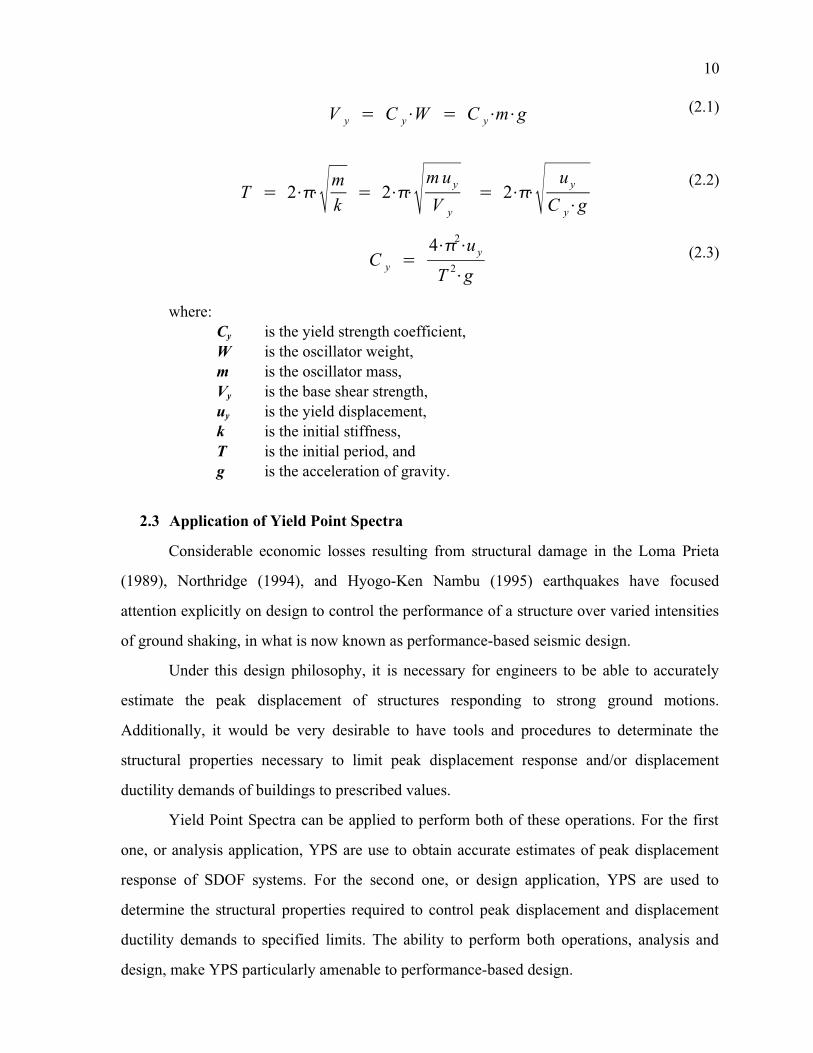
Yield Point Spectra also provide a way to easily combine peak displacement and
displacement ductility limits. Suppose it is desired to limit simultaneously the peak
displacement of an oscillator to 8 cm. or less and its displacement ductility to 4 or less. The
construction of Figure 2.5 defines a boundary that helps to identify the area of admissible
combinations of strength and stiffness that result in an approximate peak displacement less
than or equal to 8 cm. Figure 2.6 shows the inadmissible region shaded by vertical lines.
Displacement ductility demands can be controlled by simply choosing a yield point
located on or beyond the constant ductility curve representing the prescribed ductility limit.
Figure 2.7 identifies the area of inadmissible combinations of strength and stiffness that
result in a displacement ductility demand of 4 or more shaded by horizontal lines.
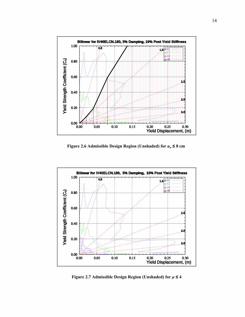
Superposition of Figures 2.6 and 2.7 results in the admissible design region, shown
unshaded in Figure 2.8, which represents combinations of strength and stiffness that satisfy
constraints on both peak displacement and displacement ductility demands.
Section 2.3.1 and 2.3.2 establish that Yield Point Spectra can be used for both
analysis and design operations: estimating peak displacement (analysis) and determining the
required combinations of strength-stiffness to limit peak displacement of SDOF to prescribed
values (design ).
Figure 2.5 Curve Defining Strength and Stiffness Combination to Limit uu to 8 cm
0.00
0.20
0.40
0.60
0.80
1.00
0.00 0.05 0.10 0.15 0.20 0.25 0.30
Bilinear for IV40ELCN.180, 5% Damping, 10% Post Yield Stiffness
Yie
ld S
tren
gth
Coe
ffici
ent (
C )y
Yield Displacement, (m)
0.51.0
1.5
2.0
3.0
µ=1µ=2µ=4µ=8
0.00
0.20
0.40
0.60
0.80
1.00
0.00 0.05 0.10 0.15 0.20 0.25 0.30
Bilinear for IV40ELCN.180, 5% Damping, 10% Post Yield Stiffness
Yie
ld S
tren
gth
Coe
ffici
ent (
C )y
Yield Displacement, (m)
0.51.0
1.5
2.0
3.0
0.00
0.20
0.40
0.60
0.80
1.00
0.00 0.05 0.10 0.15 0.20 0.25 0.30
Bilinear for IV40ELCN.180, 5% Damping, 10% Post Yield Stiffness
Yie
ld S
tren
gth
Coe
ffici
ent (
C )y
Yield Displacement, (m)
0.51.0
1.5
2.0
3.0
0.00
0.20
0.40
0.60
0.80
1.00
0.00 0.05 0.10 0.15 0.20 0.25 0.30
Bilinear for IV40ELCN.180, 5% Damping, 10% Post Yield Stiffness
Yie
ld S
tren
gth
Coe
ffici
ent (
C )y
Yield Displacement, (m)
0.51.0
1.5
2.0
3.0
0.00
0.20
0.40
0.60
0.80
1.00
0.00 0.05 0.10 0.15 0.20 0.25 0.30
Bilinear for IV40ELCN.180, 5% Damping, 10% Post Yield Stiffness
Yie
ld S
tren
gth
Coe
ffici
ent (
C )y
Yield Displacement, (m)
0.51.0
1.5
2.0
3.0
0.00
0.20
0.40
0.60
0.80
1.00
0.00 0.05 0.10 0.15 0.20 0.25 0.30
Bilinear for IV40ELCN.180, 5% Damping, 10% Post Yield Stiffness
Yie
ld S
tren
gth
Coe
ffici
ent (
C )y
Yield Displacement, (m)
0.51.0
1.5
2.0
3.0
14
Figure 2.6 Admissible Design Region (Unshaded) for uu ≤ 8 cm
0.00
0.20
0.40
0.60
0.80
1.00
0.00 0.05 0.10 0.15 0.20 0.25 0.30
Bilinear for IV40ELCN.180, 5% Damping, 10% Post Yield Stiffness
Yie
ld S
tren
gth
Coe
ffici
ent (
C )y
Yield Displacement, (m)
0.51.0
1.5
2.0
3.0
µ=1µ=2µ=4µ=8
0.00
0.20
0.40
0.60
0.80
1.00
0.00 0.05 0.10 0.15 0.20 0.25 0.30
Bilinear for IV40ELCN.180, 5% Damping, 10% Post Yield Stiffness
Yie
ld S
tren
gth
Coe
ffici
ent (
C )y
Yield Displacement, (m)
0.51.0
1.5
2.0
3.0
0.00
0.20
0.40
0.60
0.80
1.00
0.00 0.05 0.10 0.15 0.20 0.25 0.30
Bilinear for IV40ELCN.180, 5% Damping, 10% Post Yield Stiffness
Yie
ld S
tren
gth
Coe
ffici
ent (
C )y
Yield Displacement, (m)
0.51.0
1.5
2.0
3.0
0.00
0.20
0.40
0.60
0.80
1.00
0.00 0.05 0.10 0.15 0.20 0.25 0.30
Bilinear for IV40ELCN.180, 5% Damping, 10% Post Yield Stiffness
Yie
ld S
tren
gth
Coe
ffici
ent (
C )y
Yield Displacement, (m)
0.51.0
1.5
2.0
3.0
0.00
0.20
0.40
0.60
0.80
1.00
0.00 0.05 0.10 0.15 0.20 0.25 0.30
Bilinear for IV40ELCN.180, 5% Damping, 10% Post Yield Stiffness
Yie
ld S
tren
gth
Coe
ffici
ent (
C )y
Yield Displacement, (m)
0.51.0
1.5
2.0
3.0
0.00
0.20
0.40
0.60
0.80
1.00
0.00 0.05 0.10 0.15 0.20 0.25 0.30
Bilinear for IV40ELCN.180, 5% Damping, 10% Post Yield Stiffness
Yie
ld S
tren
gth
Coe
ffici
ent (
C )y
Yield Displacement, (m)
0.51.0
1.5
2.0
3.0
Figure 2.7 Admissible Design Region (Unshaded) for ≤ 4
0.00
0.20
0.40
0.60
0.80
1.00
0.00 0.05 0.10 0.15 0.20 0.25 0.30
Bilinear for IV40ELCN.180, 5% Damping, 10% Post Yield Stiffness
Yie
ld S
tren
gth
Coe
ffici
ent (
C )y
Yield Displacement, (m)
0.51.0
1.5
2.0
3.0
µ=1µ=2µ=4µ=8
0.00
0.20
0.40
0.60
0.80
1.00
0.00 0.05 0.10 0.15 0.20 0.25 0.30
Bilinear for IV40ELCN.180, 5% Damping, 10% Post Yield Stiffness
Yie
ld S
tren
gth
Coe
ffici
ent (
C )y
Yield Displacement, (m)
0.51.0
1.5
2.0
3.0
0.00
0.20
0.40
0.60
0.80
1.00
0.00 0.05 0.10 0.15 0.20 0.25 0.30
Bilinear for IV40ELCN.180, 5% Damping, 10% Post Yield Stiffness
Yie
ld S
tren
gth
Coe
ffici
ent (
C )y
Yield Displacement, (m)
0.51.0
1.5
2.0
3.0
0.00
0.20
0.40
0.60
0.80
1.00
0.00 0.05 0.10 0.15 0.20 0.25 0.30
Bilinear for IV40ELCN.180, 5% Damping, 10% Post Yield Stiffness
Yie
ld S
tren
gth
Coe
ffici
ent (
C )y
Yield Displacement, (m)
0.51.0
1.5
2.0
3.0
0.00
0.20
0.40
0.60
0.80
1.00
0.00 0.05 0.10 0.15 0.20 0.25 0.30
Bilinear for IV40ELCN.180, 5% Damping, 10% Post Yield Stiffness
Yie
ld S
tren
gth
Coe
ffici
ent (
C )y
Yield Displacement, (m)
0.51.0
1.5
2.0
3.0
0.00
0.20
0.40
0.60
0.80
1.00
0.00 0.05 0.10 0.15 0.20 0.25 0.30
Bilinear for IV40ELCN.180, 5% Damping, 10% Post Yield Stiffness
Yie
ld S
tren
gth
Coe
ffici
ent (
C )y
Yield Displacement, (m)
0.51.0
1.5
2.0
3.0
15
2.3.3 Application to Performance-Based Design
Performance-based design provides a framework to control structural performance
over a range of contemplated ground shaking intensities. Under this framework, a
performance level is described in terms of the degree of damage or functionality of the
structure for a specific intensity or likelihood of ground shaking. A performance objective is
defined as a performance levels associated with a ground motion intensity. Performance
objectives in Vision 2000 (1995) are shown in Figure 2.9.
Performance levels can be associated with numeric values of roof drift and qualitative
description of damage to components of the gravity and lateral force resisting systems.
Constraints on inter-story drift indices and system displacement ductility can be related to
limits on peak displacement response. Similarly, qualitative descriptions of damage can be
associated with local member ductility demands and those can be related to system ductility.
This allows a performance level to be expressed as a constraint on peak displacement
response and system ductility demand.
Figure 2.8 Admissible Design Region (Unshaded) for ≤ 4 and uu ≤ 8 cm
0.00
0.20
0.40
0.60
0.80
1.00
0.00 0.05 0.10 0.15 0.20 0.25 0.30
Bilinear for IV40ELCN.180, 5% Damping, 10% Post Yield Stiffness
Yie
ld S
tren
gth
Coe
ffici
ent (
C )y
Yield Displacement, (m)
0.51.0
1.5
2.0
3.0
µ=1µ=2µ=4µ=8
0.00
0.20
0.40
0.60
0.80
1.00
0.00 0.05 0.10 0.15 0.20 0.25 0.30
Bilinear for IV40ELCN.180, 5% Damping, 10% Post Yield Stiffness
Yie
ld S
tren
gth
Coe
ffici
ent (
C )y
Yield Displacement, (m)
0.51.0
1.5
2.0
3.0
0.00
0.20
0.40
0.60
0.80
1.00
0.00 0.05 0.10 0.15 0.20 0.25 0.30
Bilinear for IV40ELCN.180, 5% Damping, 10% Post Yield Stiffness
Yie
ld S
tren
gth
Coe
ffici
ent (
C )y
Yield Displacement, (m)
0.51.0
1.5
2.0
3.0
0.00
0.20
0.40
0.60
0.80
1.00
0.00 0.05 0.10 0.15 0.20 0.25 0.30
Bilinear for IV40ELCN.180, 5% Damping, 10% Post Yield Stiffness
Yie
ld S
tren
gth
Coe
ffici
ent (
C )y
Yield Displacement, (m)
0.51.0
1.5
2.0
3.0
0.00
0.20
0.40
0.60
0.80
1.00
0.00 0.05 0.10 0.15 0.20 0.25 0.30
Bilinear for IV40ELCN.180, 5% Damping, 10% Post Yield Stiffness
Yie
ld S
tren
gth
Coe
ffici
ent (
C )y
Yield Displacement, (m)
0.51.0
1.5
2.0
3.0
0.00
0.20
0.40
0.60
0.80
1.00
0.00 0.05 0.10 0.15 0.20 0.25 0.30
Bilinear for IV40ELCN.180, 5% Damping, 10% Post Yield Stiffness
Yie
ld S
tren
gth
Coe
ffici
ent (
C )y
Yield Displacement, (m)
0.51.0
1.5
2.0
3.0

16
In section 2.3.2 YPS were used to determine an admissible design region that limited
peak displacement and ductility demands to arbitrary values that may be associated with a
performance level and shaking intensity. This process can be repeated for a set of
performance levels and associated shaking intensities corresponding to a series of
performance objectives. An admissible design region that satisfies the performance
objectives is constructed by superposing the inadmissible design regions determined for each
combination of performance levels and shaking intensities. A yield point that lies within the
admissible design region satisfies the series of performance objective.
Section 2.6.2 contains a numerical example that helps to illustrate the potential use of
Yield Point Spectra in performance-based design.
2.4 Yield Point Spectra and Design Procedures
2.4.1 Conventional Design Procedures
Most seismic design at present is done by elastic methods using equivalent static
design lateral forces. In this conventional seismic design procedure, the period of vibration is
the key parameter to start the design process. Code provisions allow the fundamental period
to be approximated using formulas that depend only on the building height and the type of
lateral force resisting system employed. Once the period has been estimated, the required
Building Performance Levels
FullyOperational
Operational Life Safe Near Collapse
Frequent
(43 Years) .Occasional
(72 Years) . .Rare
(475 Years) . . .Very Rare
(970 Years) . . . .Figure 2.9 Seismic Performance Design Objective Matrix
SEAOC Vision 2000 [1995]
Ear
thqu
ake
Des
ign
Lev
els
(rec
urre
nce
inte
rval
)
Safety Critical Objectives
Essential/Hazardous Objectives
Basic Objectives

17
base shear strength is calculated using strength coefficients obtained from a smooth elastic
response spectrum reduced by a strength-reduction factor (R). The design base shear force is
distributed vertically along the building height as lateral forces. These lateral forces are used
to determine members sizes and strengths.
In general, the fundamental period calculated for the final design of the building will
be different from the approximate period used to start the design. Ideally, an iterative process
should be used to obtain a new estimate of the required strength determined using the current
fundamental period of the building. The iterations would end when the required lateral
strength is stable. This iterative process is not done in routine practice; instead codified
estimations of periods are used regardless of actual strength and stiffness.
2.4.2 Yield Displacement as Key Parameter For Design
In many practical design situations, changes in lateral strength are achieved by
changing member cross sections. These changes in strength induce changes in stiffness and
hence in periods of vibration. Only in unusual cases, such as when the grade of steel is
changed, can strength be changed without a change in stiffness.
Members depths are commonly established early in the design process and usually
change little. If changes in lateral strength are achieved by holding member depths constant
while wide flange area (steel) or steel reinforcement content (concrete) are adjusted, the yield
displacement remains nearly constant. This is because yield displacements are kinematically
determined by the properties of the constituents material(s) and the member geometry. A
simple case is a stocky column under axial load. An increase in the cross-sectional area of the
column will increase both strength and stiffness, but the yield displacement remains
unchanged. In a similar way, for predominantly flexural members, yield displacement is
determined by material properties and section depth. This observation is general and, if
member depths, materials (e.g. grade of steel), and the relative distribution of strength and
stiffness remain nearly constant, can be extended to structures having multiple members.
To illustrate the idea that changes in lateral strength influence stiffness and hence
periods, but have little effect on yield displacement, two capacity curves are presented in
Figure 2.6. The capacity curves were determined applying a displacement pattern
18
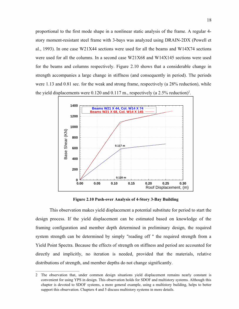
proportional to the first mode shape in a nonlinear static analysis of the frame. A regular 4-
story moment-resistant steel frame with 3-bays was analyzed using DRAIN-2DX (Powell et
al., 1993). In one case W21X44 sections were used for all the beams and W14X74 sections
were used for all the columns. In a second case W21X68 and W14X145 sections were used
for the beams and columns respectively. Figure 2.10 shows that a considerable change in
strength accompanies a large change in stiffness (and consequently in period). The periods
were 1.13 and 0.81 sec. for the weak and strong frame, respectively (a 28% reduction), while
the yield displacements were 0.120 and 0.117 m., respectively (a 2.5% reduction)2.
This observation makes yield displacement a potential substitute for period to start the
design process. If the yield displacement can be estimated based on knowledge of the
framing configuration and member depth determined in preliminary design, the required
system strength can be determined by simply "reading off " the required strength from a
Yield Point Spectra. Because the effects of strength on stiffness and period are accounted for
directly and implicitly, no iteration is needed, provided that the materials, relative
distributions of strength, and member depths do not change significantly.
2 The observation that, under common design situations yield displacement remains nearly constant isconvenient for using YPS in design. This observation holds for SDOF and multistory systems. Although thischapter is devoted to SDOF systems, a more general example, using a multistory building, helps to bettersupport this observation. Chapters 4 and 5 discuss multistory systems in more details.
Figure 2.10 Push-over Analysis of 4-Story 3-Bay Building
0
200
400
600
800
1000
1200
1400
0.00 0.05 0.10 0.15 0.20 0.25 0.30
Bas
e S
hear
(K
N)
Roof Displacement, (m)
0.120 m
0.117 m
Beams W21 X 44, Col. W14 X 74Beams W21 X 68, Col. W14 X 145

19
2.5 Strength Demands and Strength-Reduction (R) Factors
Current seismic design approaches have developed from the perspective that a
structure may have less than the strength required for elastic response if it is provided with
sufficient ductility capacity. Perhaps because of this perspective, it is common for design
procedures to relate the strength of the inelastic structure to an elastic spectrum using
strength-reduction factors (R). While the traditional strength-reduction factor is a single-
valued relationship for a given structural system, many researchers (e.g. Miranda and Bertero
1994; Nassar and Krawinkler, 1991; Newmark and Hall, 1982) have expressed strength-
reduction factors as a function of period of vibration (T).
The strength-reduction factor is defined as the ratio of the force that would develop
under the specified ground motion if the structure had an entirely linear elastic response, to
the prescribed design forces. In typical cases the strength-reduction factor is larger than 1.0;
thus, typically structures are designed for forces smaller than those the design earthquake
would produce in a completely linear-elastic responding structure (FEMA 303; 1997).
Consequently, the design base shear strength is often expressed as a function of the elastic
spectral acceleration divided by a strength-reduction factor.
In conventional design procedures, the strength-reduction factor and the elastic
response spectra are positive for all periods. Therefore, some lateral strength is required
regardless of the period of the structure. Additionally, it is accepted that the larger the
strength-reduction factor is the larger the ductility demands.
Yield Point Spectra allow one to identify two consistent trends, derived from the use
of yield displacement as primary variable for assessing strength requirements (Section 2.4.2),
that question these common views. These trends will be explained using Figure 2.11, and are
supported by the YPS prepared for 15 ground motions for both bilinear and stiffness
degrading load-deformation models (Figures 2.18-2.20). These ground motions and the load-
deformation models are described in Section 2.7.
In Figure 2.11, the Yield Point Spectra for the N-S 1940 El Centro record is shown in
log-log format. Using this format, lines of constant period plot as paralel diagonal lines. Data
supporting conventional period-based formulations can be recovered by reading the YPS
along these lines of constant periods.
20
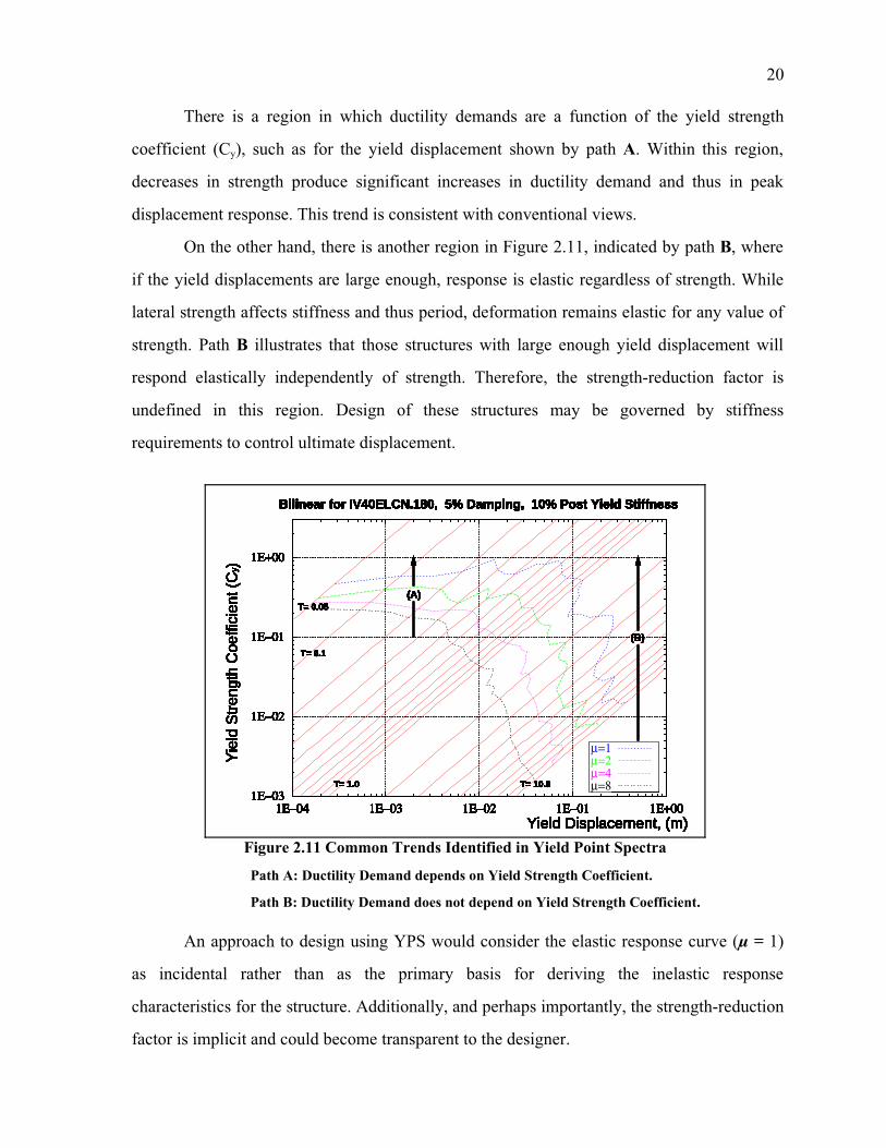
There is a region in which ductility demands are a function of the yield strength
coefficient (Cy), such as for the yield displacement shown by path A. Within this region,
decreases in strength produce significant increases in ductility demand and thus in peak
displacement response. This trend is consistent with conventional views.
On the other hand, there is another region in Figure 2.11, indicated by path B, where
if the yield displacements are large enough, response is elastic regardless of strength. While
lateral strength affects stiffness and thus period, deformation remains elastic for any value of
strength. Path B illustrates that those structures with large enough yield displacement will
respond elastically independently of strength. Therefore, the strength-reduction factor is
undefined in this region. Design of these structures may be governed by stiffness
requirements to control ultimate displacement.
An approach to design using YPS would consider the elastic response curve ( = 1)
as incidental rather than as the primary basis for deriving the inelastic response
characteristics for the structure. Additionally, and perhaps importantly, the strength-reduction
factor is implicit and could become transparent to the designer.
Figure 2.11 Common Trends Identified in Yield Point Spectra
Path A: Ductility Demand depends on Yield Strength Coefficient.
Path B: Ductility Demand does not depend on Yield Strength Coefficient.
1Ε−03
1Ε−02
1Ε−01
1Ε+00
1Ε−04 1Ε−03 1Ε−02 1Ε−01 1Ε+00
Bilinear for IV40ELCN.180, 5% Damping, 10% Post Yield Stiffness
Yie
ld S
tren
gth
Coe
ffici
ent (
C )y
Yield Displacement, (m)
T= 0.05
T= 0.1
T= 1.0 T= 10.0
(A)
(B)
µ=1µ=2µ=4µ=8
1Ε−03
1Ε−02
1Ε−01
1Ε+00
1Ε−04 1Ε−03 1Ε−02 1Ε−01 1Ε+00
Bilinear for IV40ELCN.180, 5% Damping, 10% Post Yield Stiffness
Yie
ld S
tren
gth
Coe
ffici
ent (
C )y
Yield Displacement, (m)
T= 0.05
T= 0.1
T= 1.0 T= 10.0
(A)
(B)
1Ε−03
1Ε−02
1Ε−01
1Ε+00
1Ε−04 1Ε−03 1Ε−02 1Ε−01 1Ε+00
Bilinear for IV40ELCN.180, 5% Damping, 10% Post Yield Stiffness
Yie
ld S
tren
gth
Coe
ffici
ent (
C )y
Yield Displacement, (m)
T= 0.05
T= 0.1
T= 1.0 T= 10.0
(A)
(B)
1Ε−03
1Ε−02
1Ε−01
1Ε+00
1Ε−04 1Ε−03 1Ε−02 1Ε−01 1Ε+00
Bilinear for IV40ELCN.180, 5% Damping, 10% Post Yield Stiffness
Yie
ld S
tren
gth
Coe
ffici
ent (
C )y
Yield Displacement, (m)
T= 0.05
T= 0.1
T= 1.0 T= 10.0
(A)
(B)
1Ε−03
1Ε−02
1Ε−01
1Ε+00
1Ε−04 1Ε−03 1Ε−02 1Ε−01 1Ε+00
Bilinear for IV40ELCN.180, 5% Damping, 10% Post Yield Stiffness
Yie
ld S
tren
gth
Coe
ffici
ent (
C )y
Yield Displacement, (m)
T= 0.05
T= 0.1
T= 1.0 T= 10.0
(A)
(B)
1Ε−03
1Ε−02
1Ε−01
1Ε+00
1Ε−04 1Ε−03 1Ε−02 1Ε−01 1Ε+00
Bilinear for IV40ELCN.180, 5% Damping, 10% Post Yield Stiffness
Yie
ld S
tren
gth
Coe
ffici
ent (
C )y
Yield Displacement, (m)
T= 0.05
T= 0.1
T= 1.0 T= 10.0
(A)
(B)
1Ε−03
1Ε−02
1Ε−01
1Ε+00
1Ε−04 1Ε−03 1Ε−02 1Ε−01 1Ε+00
Bilinear for IV40ELCN.180, 5% Damping, 10% Post Yield Stiffness
Yie
ld S
tren
gth
Coe
ffici
ent (
C )y
Yield Displacement, (m)
T= 0.05
T= 0.1
T= 1.0 T= 10.0
(A)
(B)
1Ε−03
1Ε−02
1Ε−01
1Ε+00
1Ε−04 1Ε−03 1Ε−02 1Ε−01 1Ε+00
Bilinear for IV40ELCN.180, 5% Damping, 10% Post Yield Stiffness
Yie
ld S
tren
gth
Coe
ffici
ent (
C )y
Yield Displacement, (m)
T= 0.05
T= 0.1
T= 1.0 T= 10.0
(A)
(B)
1Ε−03
1Ε−02
1Ε−01
1Ε+00
1Ε−04 1Ε−03 1Ε−02 1Ε−01 1Ε+00
Bilinear for IV40ELCN.180, 5% Damping, 10% Post Yield Stiffness
Yie
ld S
tren
gth
Coe
ffici
ent (
C )y
Yield Displacement, (m)
T= 0.05
T= 0.1
T= 1.0 T= 10.0
(A)
(B)
1Ε−03
1Ε−02
1Ε−01
1Ε+00
1Ε−04 1Ε−03 1Ε−02 1Ε−01 1Ε+00
Bilinear for IV40ELCN.180, 5% Damping, 10% Post Yield Stiffness
Yie
ld S
tren
gth
Coe
ffici
ent (
C )y
Yield Displacement, (m)
T= 0.05
T= 0.1
T= 1.0 T= 10.0
(A)
(B)
1Ε−03
1Ε−02
1Ε−01
1Ε+00
1Ε−04 1Ε−03 1Ε−02 1Ε−01 1Ε+00
Bilinear for IV40ELCN.180, 5% Damping, 10% Post Yield Stiffness
Yie
ld S
tren
gth
Coe
ffici
ent (
C )y
Yield Displacement, (m)
T= 0.05
T= 0.1
T= 1.0 T= 10.0
(A)
(B)
1Ε−03
1Ε−02
1Ε−01
1Ε+00
1Ε−04 1Ε−03 1Ε−02 1Ε−01 1Ε+00
Bilinear for IV40ELCN.180, 5% Damping, 10% Post Yield Stiffness
Yie
ld S
tren
gth
Coe
ffici
ent (
C )y
Yield Displacement, (m)
T= 0.05
T= 0.1
T= 1.0 T= 10.0
(A)
(B)
1Ε−03
1Ε−02
1Ε−01
1Ε+00
1Ε−04 1Ε−03 1Ε−02 1Ε−01 1Ε+00
Bilinear for IV40ELCN.180, 5% Damping, 10% Post Yield Stiffness
Yie
ld S
tren
gth
Coe
ffici
ent (
C )y
Yield Displacement, (m)
T= 0.05
T= 0.1
T= 1.0 T= 10.0
(A)
(B)
1Ε−03
1Ε−02
1Ε−01
1Ε+00
1Ε−04 1Ε−03 1Ε−02 1Ε−01 1Ε+00
Bilinear for IV40ELCN.180, 5% Damping, 10% Post Yield Stiffness
Yie
ld S
tren
gth
Coe
ffici
ent (
C )y
Yield Displacement, (m)
T= 0.05
T= 0.1
T= 1.0 T= 10.0
(A)
(B)
1Ε−03
1Ε−02
1Ε−01
1Ε+00
1Ε−04 1Ε−03 1Ε−02 1Ε−01 1Ε+00
Bilinear for IV40ELCN.180, 5% Damping, 10% Post Yield Stiffness
Yie
ld S
tren
gth
Coe
ffici
ent (
C )y
Yield Displacement, (m)
T= 0.05
T= 0.1
T= 1.0 T= 10.0
(A)
(B)
1Ε−03
1Ε−02
1Ε−01
1Ε+00
1Ε−04 1Ε−03 1Ε−02 1Ε−01 1Ε+00
Bilinear for IV40ELCN.180, 5% Damping, 10% Post Yield Stiffness
Yie
ld S
tren
gth
Coe
ffici
ent (
C )y
Yield Displacement, (m)
T= 0.05
T= 0.1
T= 1.0 T= 10.0
(A)
(B)
1Ε−03
1Ε−02
1Ε−01
1Ε+00
1Ε−04 1Ε−03 1Ε−02 1Ε−01 1Ε+00
Bilinear for IV40ELCN.180, 5% Damping, 10% Post Yield Stiffness
Yie
ld S
tren
gth
Coe
ffici
ent (
C )y
Yield Displacement, (m)
T= 0.05
T= 0.1
T= 1.0 T= 10.0
(A)
(B)
1Ε−03
1Ε−02
1Ε−01
1Ε+00
1Ε−04 1Ε−03 1Ε−02 1Ε−01 1Ε+00
Bilinear for IV40ELCN.180, 5% Damping, 10% Post Yield Stiffness
Yie
ld S
tren
gth
Coe
ffici
ent (
C )y
Yield Displacement, (m)
T= 0.05
T= 0.1
T= 1.0 T= 10.0
(A)
(B)
1Ε−03
1Ε−02
1Ε−01
1Ε+00
1Ε−04 1Ε−03 1Ε−02 1Ε−01 1Ε+00
Bilinear for IV40ELCN.180, 5% Damping, 10% Post Yield Stiffness
Yie
ld S
tren
gth
Coe
ffici
ent (
C )y
Yield Displacement, (m)
T= 0.05
T= 0.1
T= 1.0 T= 10.0
(A)
(B)
1Ε−03
1Ε−02
1Ε−01
1Ε+00
1Ε−04 1Ε−03 1Ε−02 1Ε−01 1Ε+00
Bilinear for IV40ELCN.180, 5% Damping, 10% Post Yield Stiffness
Yie
ld S
tren
gth
Coe
ffici
ent (
C )y
Yield Displacement, (m)
T= 0.05
T= 0.1
T= 1.0 T= 10.0
(A)
(B)
1Ε−03
1Ε−02
1Ε−01
1Ε+00
1Ε−04 1Ε−03 1Ε−02 1Ε−01 1Ε+00
Bilinear for IV40ELCN.180, 5% Damping, 10% Post Yield Stiffness
Yie
ld S
tren
gth
Coe
ffici
ent (
C )y
Yield Displacement, (m)
T= 0.05
T= 0.1
T= 1.0 T= 10.0
(A)
(B)

21
2.6 Numerical Examples
To better support the ideas discussed in this chapter, two numerical examples are
presented in this section. The first is intended to show accuracy in peak displacement and
displacement ductility estimates made using YPS. The second example illustrates how Yield
Point Spectra can be used in performance-based design.
2.6.1 Example 1. Accuracy of YPS Estimates
The peak displacement and displacement ductility responses of three SDOF
oscillators are estimated using Yield Point Spectra computed for the N-S 1940 El Centro
record. The oscillators have a bilinear load-deformation model with post-yield stiffness equal
to 10% of the initial stiffness; damping was to 5% of critical damping.
The yield displacement for the first oscillator is 2 cm. (0.02 m), the second has a yield
displacement of 1.5 cm. and the third has a yield displacement of 3.0 cm. One additional
parameter, either the initial period or the strength (Cy) of the system, is needed to read
ductility demands from the Yield Point Spectra of Figure 2.12. For illustration purposes only,
the initial period of the first two oscillators is set to 1.0 sec, and for the third oscillator the
yield strength coefficient was assumed equal to 3%.
Figure 2.12 shows that for the first oscillator, an arrow representing a yield
displacement of 2 cm. intersects the 1.0 sec. period line (diagonal lines represent initial
periods) at the curve corresponding to a ductility demand of 4. Therefore, this oscillator will
respond to this earthquake with a ductility demand approximately equal to 4 and sustain a
peak displacement equal to 4 times its yield displacement (~ 8 cm.).
For the second oscillator, Figure 2.12 shows that the arrow representing its yield
displacement (1.5 cm.) intersects the 1.0 sec. period line between the curves corresponding to
ductility demand of 4 and 8. Here, it is important to notice that these constant ductility curves
are powers of two (20, 21, 22, 23) and that they are approximately evenly spaced in the log-log
format of Figure 2.12. Then, for this oscillator the ductility should be read for a point that is
approximately at 45% of the distance measured from the curve of a ductility of 4 (22) toward
the curve of a ductility of 8 (23). The displacement ductility demand can therefore be
estimated as 22.45 = 5.46. Thus, the peak displacement is approximately (1.5) (5.46) = 8.2 cm.
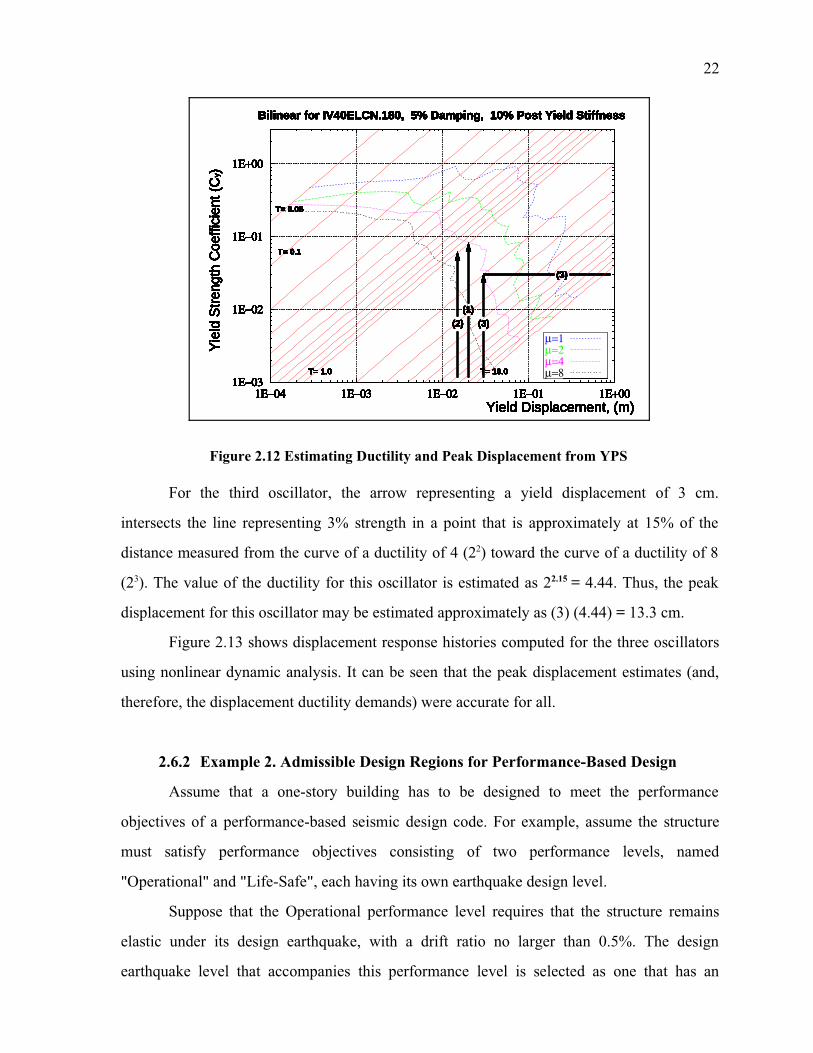
22
For the third oscillator, the arrow representing a yield displacement of 3 cm.
intersects the line representing 3% strength in a point that is approximately at 15% of the
distance measured from the curve of a ductility of 4 (22) toward the curve of a ductility of 8
(23). The value of the ductility for this oscillator is estimated as 22.15 = 4.44. Thus, the peak
displacement for this oscillator may be estimated approximately as (3) (4.44) = 13.3 cm.
Figure 2.13 shows displacement response histories computed for the three oscillators
using nonlinear dynamic analysis. It can be seen that the peak displacement estimates (and,
therefore, the displacement ductility demands) were accurate for all.
2.6.2 Example 2. Admissible Design Regions for Performance-Based Design
Assume that a one-story building has to be designed to meet the performance
objectives of a performance-based seismic design code. For example, assume the structure
must satisfy performance objectives consisting of two performance levels, named
"Operational" and "Life-Safe", each having its own earthquake design level.
Suppose that the Operational performance level requires that the structure remains
elastic under its design earthquake, with a drift ratio no larger than 0.5%. The design
earthquake level that accompanies this performance level is selected as one that has an
Figure 2.12 Estimating Ductility and Peak Displacement from YPS
1Ε−03
1Ε−02
1Ε−01
1Ε+00
1Ε−04 1Ε−03 1Ε−02 1Ε−01 1Ε+00
Bilinear for IV40ELCN.180, 5% Damping, 10% Post Yield Stiffness
Yie
ld S
tren
gth
Coe
ffici
ent (
C )y
Yield Displacement, (m)
T= 0.05
T= 0.1
T= 1.0 T= 10.0
(1)
(2) (3)
(3)
µ=1µ=2µ=4µ=8
1Ε−03
1Ε−02
1Ε−01
1Ε+00
1Ε−04 1Ε−03 1Ε−02 1Ε−01 1Ε+00
Bilinear for IV40ELCN.180, 5% Damping, 10% Post Yield Stiffness
Yie
ld S
tren
gth
Coe
ffici
ent (
C )y
Yield Displacement, (m)
T= 0.05
T= 0.1
T= 1.0 T= 10.0
(1)
(2) (3)
(3)
1Ε−03
1Ε−02
1Ε−01
1Ε+00
1Ε−04 1Ε−03 1Ε−02 1Ε−01 1Ε+00
Bilinear for IV40ELCN.180, 5% Damping, 10% Post Yield Stiffness
Yie
ld S
tren
gth
Coe
ffici
ent (
C )y
Yield Displacement, (m)
T= 0.05
T= 0.1
T= 1.0 T= 10.0
(1)
(2) (3)
(3)
1Ε−03
1Ε−02
1Ε−01
1Ε+00
1Ε−04 1Ε−03 1Ε−02 1Ε−01 1Ε+00
Bilinear for IV40ELCN.180, 5% Damping, 10% Post Yield Stiffness
Yie
ld S
tren
gth
Coe
ffici
ent (
C )y
Yield Displacement, (m)
T= 0.05
T= 0.1
T= 1.0 T= 10.0
(1)
(2) (3)
(3)
1Ε−03
1Ε−02
1Ε−01
1Ε+00
1Ε−04 1Ε−03 1Ε−02 1Ε−01 1Ε+00
Bilinear for IV40ELCN.180, 5% Damping, 10% Post Yield Stiffness
Yie
ld S
tren
gth
Coe
ffici
ent (
C )y
Yield Displacement, (m)
T= 0.05
T= 0.1
T= 1.0 T= 10.0
(1)
(2) (3)
(3)
1Ε−03
1Ε−02
1Ε−01
1Ε+00
1Ε−04 1Ε−03 1Ε−02 1Ε−01 1Ε+00
Bilinear for IV40ELCN.180, 5% Damping, 10% Post Yield Stiffness
Yie
ld S
tren
gth
Coe
ffici
ent (
C )y
Yield Displacement, (m)
T= 0.05
T= 0.1
T= 1.0 T= 10.0
(1)
(2) (3)
(3)
1Ε−03
1Ε−02
1Ε−01
1Ε+00
1Ε−04 1Ε−03 1Ε−02 1Ε−01 1Ε+00
Bilinear for IV40ELCN.180, 5% Damping, 10% Post Yield Stiffness
Yie
ld S
tren
gth
Coe
ffici
ent (
C )y
Yield Displacement, (m)
T= 0.05
T= 0.1
T= 1.0 T= 10.0
(1)
(2) (3)
(3)
1Ε−03
1Ε−02
1Ε−01
1Ε+00
1Ε−04 1Ε−03 1Ε−02 1Ε−01 1Ε+00
Bilinear for IV40ELCN.180, 5% Damping, 10% Post Yield Stiffness
Yie
ld S
tren
gth
Coe
ffici
ent (
C )y
Yield Displacement, (m)
T= 0.05
T= 0.1
T= 1.0 T= 10.0
(1)
(2) (3)
(3)
1Ε−03
1Ε−02
1Ε−01
1Ε+00
1Ε−04 1Ε−03 1Ε−02 1Ε−01 1Ε+00
Bilinear for IV40ELCN.180, 5% Damping, 10% Post Yield Stiffness
Yie
ld S
tren
gth
Coe
ffici
ent (
C )y
Yield Displacement, (m)
T= 0.05
T= 0.1
T= 1.0 T= 10.0
(1)
(2) (3)
(3)
1Ε−03
1Ε−02
1Ε−01
1Ε+00
1Ε−04 1Ε−03 1Ε−02 1Ε−01 1Ε+00
Bilinear for IV40ELCN.180, 5% Damping, 10% Post Yield Stiffness
Yie
ld S
tren
gth
Coe
ffici
ent (
C )y
Yield Displacement, (m)
T= 0.05
T= 0.1
T= 1.0 T= 10.0
(1)
(2) (3)
(3)
1Ε−03
1Ε−02
1Ε−01
1Ε+00
1Ε−04 1Ε−03 1Ε−02 1Ε−01 1Ε+00
Bilinear for IV40ELCN.180, 5% Damping, 10% Post Yield Stiffness
Yie
ld S
tren
gth
Coe
ffici
ent (
C )y
Yield Displacement, (m)
T= 0.05
T= 0.1
T= 1.0 T= 10.0
(1)
(2) (3)
(3)
1Ε−03
1Ε−02
1Ε−01
1Ε+00
1Ε−04 1Ε−03 1Ε−02 1Ε−01 1Ε+00
Bilinear for IV40ELCN.180, 5% Damping, 10% Post Yield Stiffness
Yie
ld S
tren
gth
Coe
ffici
ent (
C )y
Yield Displacement, (m)
T= 0.05
T= 0.1
T= 1.0 T= 10.0
(1)
(2) (3)
(3)
1Ε−03
1Ε−02
1Ε−01
1Ε+00
1Ε−04 1Ε−03 1Ε−02 1Ε−01 1Ε+00
Bilinear for IV40ELCN.180, 5% Damping, 10% Post Yield Stiffness
Yie
ld S
tren
gth
Coe
ffici
ent (
C )y
Yield Displacement, (m)
T= 0.05
T= 0.1
T= 1.0 T= 10.0
(1)
(2) (3)
(3)
1Ε−03
1Ε−02
1Ε−01
1Ε+00
1Ε−04 1Ε−03 1Ε−02 1Ε−01 1Ε+00
Bilinear for IV40ELCN.180, 5% Damping, 10% Post Yield Stiffness
Yie
ld S
tren
gth
Coe
ffici
ent (
C )y
Yield Displacement, (m)
T= 0.05
T= 0.1
T= 1.0 T= 10.0
(1)
(2) (3)
(3)
1Ε−03
1Ε−02
1Ε−01
1Ε+00
1Ε−04 1Ε−03 1Ε−02 1Ε−01 1Ε+00
Bilinear for IV40ELCN.180, 5% Damping, 10% Post Yield Stiffness
Yie
ld S
tren
gth
Coe
ffici
ent (
C )y
Yield Displacement, (m)
T= 0.05
T= 0.1
T= 1.0 T= 10.0
(1)
(2) (3)
(3)
1Ε−03
1Ε−02
1Ε−01
1Ε+00
1Ε−04 1Ε−03 1Ε−02 1Ε−01 1Ε+00
Bilinear for IV40ELCN.180, 5% Damping, 10% Post Yield Stiffness
Yie
ld S
tren
gth
Coe
ffici
ent (
C )y
Yield Displacement, (m)
T= 0.05
T= 0.1
T= 1.0 T= 10.0
(1)
(2) (3)
(3)
1Ε−03
1Ε−02
1Ε−01
1Ε+00
1Ε−04 1Ε−03 1Ε−02 1Ε−01 1Ε+00
Bilinear for IV40ELCN.180, 5% Damping, 10% Post Yield Stiffness
Yie
ld S
tren
gth
Coe
ffici
ent (
C )y
Yield Displacement, (m)
T= 0.05
T= 0.1
T= 1.0 T= 10.0
(1)
(2) (3)
(3)
1Ε−03
1Ε−02
1Ε−01
1Ε+00
1Ε−04 1Ε−03 1Ε−02 1Ε−01 1Ε+00
Bilinear for IV40ELCN.180, 5% Damping, 10% Post Yield Stiffness
Yie
ld S
tren
gth
Coe
ffici
ent (
C )y
Yield Displacement, (m)
T= 0.05
T= 0.1
T= 1.0 T= 10.0
(1)
(2) (3)
(3)
1Ε−03
1Ε−02
1Ε−01
1Ε+00
1Ε−04 1Ε−03 1Ε−02 1Ε−01 1Ε+00
Bilinear for IV40ELCN.180, 5% Damping, 10% Post Yield Stiffness
Yie
ld S
tren
gth
Coe
ffici
ent (
C )y
Yield Displacement, (m)
T= 0.05
T= 0.1
T= 1.0 T= 10.0
(1)
(2) (3)
(3)
1Ε−03
1Ε−02
1Ε−01
1Ε+00
1Ε−04 1Ε−03 1Ε−02 1Ε−01 1Ε+00
Bilinear for IV40ELCN.180, 5% Damping, 10% Post Yield Stiffness
Yie
ld S
tren
gth
Coe
ffici
ent (
C )y
Yield Displacement, (m)
T= 0.05
T= 0.1
T= 1.0 T= 10.0
(1)
(2) (3)
(3)
1Ε−03
1Ε−02
1Ε−01
1Ε+00
1Ε−04 1Ε−03 1Ε−02 1Ε−01 1Ε+00
Bilinear for IV40ELCN.180, 5% Damping, 10% Post Yield Stiffness
Yie
ld S
tren
gth
Coe
ffici
ent (
C )y
Yield Displacement, (m)
T= 0.05
T= 0.1
T= 1.0 T= 10.0
(1)
(2) (3)
(3)
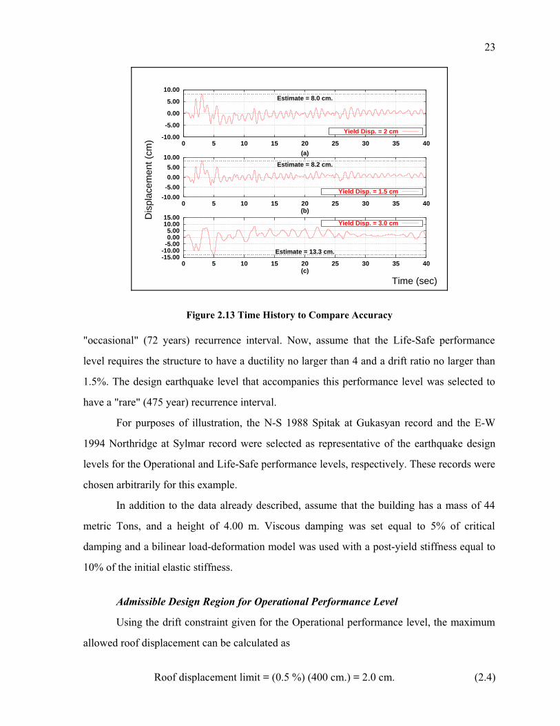
23
"occasional" (72 years) recurrence interval. Now, assume that the Life-Safe performance
level requires the structure to have a ductility no larger than 4 and a drift ratio no larger than
1.5%. The design earthquake level that accompanies this performance level was selected to
have a "rare" (475 year) recurrence interval.
For purposes of illustration, the N-S 1988 Spitak at Gukasyan record and the E-W
1994 Northridge at Sylmar record were selected as representative of the earthquake design
levels for the Operational and Life-Safe performance levels, respectively. These records were
chosen arbitrarily for this example.
In addition to the data already described, assume that the building has a mass of 44
metric Tons, and a height of 4.00 m. Viscous damping was set equal to 5% of critical
damping and a bilinear load-deformation model was used with a post-yield stiffness equal to
10% of the initial elastic stiffness.
Admissible Design Region for Operational Performance Level
Using the drift constraint given for the Operational performance level, the maximum
allowed roof displacement can be calculated as
Roof displacement limit = (0.5 %) (400 cm.) = 2.0 cm. (2.4)
Figure 2.13 Time History to Compare Accuracy
-10.00
-5.00
0.00
5.00
10.00
0 5 10 15 20 25 30 35 40D
ispl
acem
ent (
cm)
Time (sec)
Estimate = 8.0 cm.
(a)
Yield Disp. = 2 cm
-10.00
-5.00
0.00
5.00
10.00
0 5 10 15 20 25 30 35 40
Estimate = 8.2 cm.
(b)
Yield Disp. = 1.5 cm
-15.00-10.00
-5.000.005.00
10.0015.00
0 5 10 15 20 25 30 35 40
Estimate = 13.3 cm.
(c)
Yield Disp. = 3.0 cm

24
Figure 2.14 shows combinations of strength and stiffness that satisfy both ductility
and drift constraints for this performance level. Notice that Figure 2.14 is similar to Figure
2.8 in the sense that both displacement and ductility constraints are shown. The inadmissible
region is shaded by vertical lines.
The point having a yield displacement equal to the roof displacement limit (2.0 cm.)
and the minimum strength required by the structure to have an elastic response is marked
with a dark dot on Figure 2.14. This point divides the border between the admissible and
inadmissible regions into two branches. To the left of the dot is the ductility controlled
branch; any yield point below this branch represents a system that will have a ductility
demand greater than one regardless of peak displacement. To the right of the dot is the drift
controlled branch; any yield point below this branch represents a system having peak
displacement greater than the roof limit regardless of ductility demand.
• Admissible Design Region for Life-Safe Performance Level
Again, using the drift constraint for this performance level, 1.5%, the maximum
allowable roof displacement is found.
Figure 2.14 Admissible Design Region for Operational Performance Level
1Ε−03
1Ε−02
1Ε−01
1Ε+00
1Ε−04 1Ε−03 1Ε−02 1Ε−01 1Ε+00
Bilinear for SP88GUKA.360, 5% Damping, 10% Post Yield Stiffness
Yie
ld S
tren
gth
Coe
ffici
ent (
C )y
Yield Displacement, (m)
T= 0.05
T= 0.1
T= 1.0 T= 10.0
µ=1µ=2µ=4µ=8
1Ε−03
1Ε−02
1Ε−01
1Ε+00
1Ε−04 1Ε−03 1Ε−02 1Ε−01 1Ε+00
Bilinear for SP88GUKA.360, 5% Damping, 10% Post Yield Stiffness
Yie
ld S
tren
gth
Coe
ffici
ent (
C )y
Yield Displacement, (m)
T= 0.05
T= 0.1
T= 1.0 T= 10.01Ε−03
1Ε−02
1Ε−01
1Ε+00
1Ε−04 1Ε−03 1Ε−02 1Ε−01 1Ε+00
Bilinear for SP88GUKA.360, 5% Damping, 10% Post Yield Stiffness
Yie
ld S
tren
gth
Coe
ffici
ent (
C )y
Yield Displacement, (m)
T= 0.05
T= 0.1
T= 1.0 T= 10.01Ε−03
1Ε−02
1Ε−01
1Ε+00
1Ε−04 1Ε−03 1Ε−02 1Ε−01 1Ε+00
Bilinear for SP88GUKA.360, 5% Damping, 10% Post Yield Stiffness
Yie
ld S
tren
gth
Coe
ffici
ent (
C )y
Yield Displacement, (m)
T= 0.05
T= 0.1
T= 1.0 T= 10.01Ε−03
1Ε−02
1Ε−01
1Ε+00
1Ε−04 1Ε−03 1Ε−02 1Ε−01 1Ε+00
Bilinear for SP88GUKA.360, 5% Damping, 10% Post Yield Stiffness
Yie
ld S
tren
gth
Coe
ffici
ent (
C )y
Yield Displacement, (m)
T= 0.05
T= 0.1
T= 1.0 T= 10.01Ε−03
1Ε−02
1Ε−01
1Ε+00
1Ε−04 1Ε−03 1Ε−02 1Ε−01 1Ε+00
Bilinear for SP88GUKA.360, 5% Damping, 10% Post Yield Stiffness
Yie
ld S
tren
gth
Coe
ffici
ent (
C )y
Yield Displacement, (m)
T= 0.05
T= 0.1
T= 1.0 T= 10.01Ε−03
1Ε−02
1Ε−01
1Ε+00
1Ε−04 1Ε−03 1Ε−02 1Ε−01 1Ε+00
Bilinear for SP88GUKA.360, 5% Damping, 10% Post Yield Stiffness
Yie
ld S
tren
gth
Coe
ffici
ent (
C )y
Yield Displacement, (m)
T= 0.05
T= 0.1
T= 1.0 T= 10.01Ε−03
1Ε−02
1Ε−01
1Ε+00
1Ε−04 1Ε−03 1Ε−02 1Ε−01 1Ε+00
Bilinear for SP88GUKA.360, 5% Damping, 10% Post Yield Stiffness
Yie
ld S
tren
gth
Coe
ffici
ent (
C )y
Yield Displacement, (m)
T= 0.05
T= 0.1
T= 1.0 T= 10.01Ε−03
1Ε−02
1Ε−01
1Ε+00
1Ε−04 1Ε−03 1Ε−02 1Ε−01 1Ε+00
Bilinear for SP88GUKA.360, 5% Damping, 10% Post Yield Stiffness
Yie
ld S
tren
gth
Coe
ffici
ent (
C )y
Yield Displacement, (m)
T= 0.05
T= 0.1
T= 1.0 T= 10.01Ε−03
1Ε−02
1Ε−01
1Ε+00
1Ε−04 1Ε−03 1Ε−02 1Ε−01 1Ε+00
Bilinear for SP88GUKA.360, 5% Damping, 10% Post Yield Stiffness
Yie
ld S
tren
gth
Coe
ffici
ent (
C )y
Yield Displacement, (m)
T= 0.05
T= 0.1
T= 1.0 T= 10.01Ε−03
1Ε−02
1Ε−01
1Ε+00
1Ε−04 1Ε−03 1Ε−02 1Ε−01 1Ε+00
Bilinear for SP88GUKA.360, 5% Damping, 10% Post Yield Stiffness
Yie
ld S
tren
gth
Coe
ffici
ent (
C )y
Yield Displacement, (m)
T= 0.05
T= 0.1
T= 1.0 T= 10.01Ε−03
1Ε−02
1Ε−01
1Ε+00
1Ε−04 1Ε−03 1Ε−02 1Ε−01 1Ε+00
Bilinear for SP88GUKA.360, 5% Damping, 10% Post Yield Stiffness
Yie
ld S
tren
gth
Coe
ffici
ent (
C )y
Yield Displacement, (m)
T= 0.05
T= 0.1
T= 1.0 T= 10.01Ε−03
1Ε−02
1Ε−01
1Ε+00
1Ε−04 1Ε−03 1Ε−02 1Ε−01 1Ε+00
Bilinear for SP88GUKA.360, 5% Damping, 10% Post Yield Stiffness
Yie
ld S
tren
gth
Coe
ffici
ent (
C )y
Yield Displacement, (m)
T= 0.05
T= 0.1
T= 1.0 T= 10.01Ε−03
1Ε−02
1Ε−01
1Ε+00
1Ε−04 1Ε−03 1Ε−02 1Ε−01 1Ε+00
Bilinear for SP88GUKA.360, 5% Damping, 10% Post Yield Stiffness
Yie
ld S
tren
gth
Coe
ffici
ent (
C )y
Yield Displacement, (m)
T= 0.05
T= 0.1
T= 1.0 T= 10.01Ε−03
1Ε−02
1Ε−01
1Ε+00
1Ε−04 1Ε−03 1Ε−02 1Ε−01 1Ε+00
Bilinear for SP88GUKA.360, 5% Damping, 10% Post Yield Stiffness
Yie
ld S
tren
gth
Coe
ffici
ent (
C )y
Yield Displacement, (m)
T= 0.05
T= 0.1
T= 1.0 T= 10.01Ε−03
1Ε−02
1Ε−01
1Ε+00
1Ε−04 1Ε−03 1Ε−02 1Ε−01 1Ε+00
Bilinear for SP88GUKA.360, 5% Damping, 10% Post Yield Stiffness
Yie
ld S
tren
gth
Coe
ffici
ent (
C )y
Yield Displacement, (m)
T= 0.05
T= 0.1
T= 1.0 T= 10.01Ε−03
1Ε−02
1Ε−01
1Ε+00
1Ε−04 1Ε−03 1Ε−02 1Ε−01 1Ε+00
Bilinear for SP88GUKA.360, 5% Damping, 10% Post Yield Stiffness
Yie
ld S
tren
gth
Coe
ffici
ent (
C )y
Yield Displacement, (m)
T= 0.05
T= 0.1
T= 1.0 T= 10.01Ε−03
1Ε−02
1Ε−01
1Ε+00
1Ε−04 1Ε−03 1Ε−02 1Ε−01 1Ε+00
Bilinear for SP88GUKA.360, 5% Damping, 10% Post Yield Stiffness
Yie
ld S
tren
gth
Coe
ffici
ent (
C )y
Yield Displacement, (m)
T= 0.05
T= 0.1
T= 1.0 T= 10.01Ε−03
1Ε−02
1Ε−01
1Ε+00
1Ε−04 1Ε−03 1Ε−02 1Ε−01 1Ε+00
Bilinear for SP88GUKA.360, 5% Damping, 10% Post Yield Stiffness
Yie
ld S
tren
gth
Coe
ffici
ent (
C )y
Yield Displacement, (m)
T= 0.05
T= 0.1
T= 1.0 T= 10.01Ε−03
1Ε−02
1Ε−01
1Ε+00
1Ε−04 1Ε−03 1Ε−02 1Ε−01 1Ε+00
Bilinear for SP88GUKA.360, 5% Damping, 10% Post Yield Stiffness
Yie
ld S
tren
gth
Coe
ffici
ent (
C )y
Yield Displacement, (m)
T= 0.05
T= 0.1
T= 1.0 T= 10.01Ε−03
1Ε−02
1Ε−01
1Ε+00
1Ε−04 1Ε−03 1Ε−02 1Ε−01 1Ε+00
Bilinear for SP88GUKA.360, 5% Damping, 10% Post Yield Stiffness
Yie
ld S
tren
gth
Coe
ffici
ent (
C )y
Yield Displacement, (m)
T= 0.05
T= 0.1
T= 1.0 T= 10.0
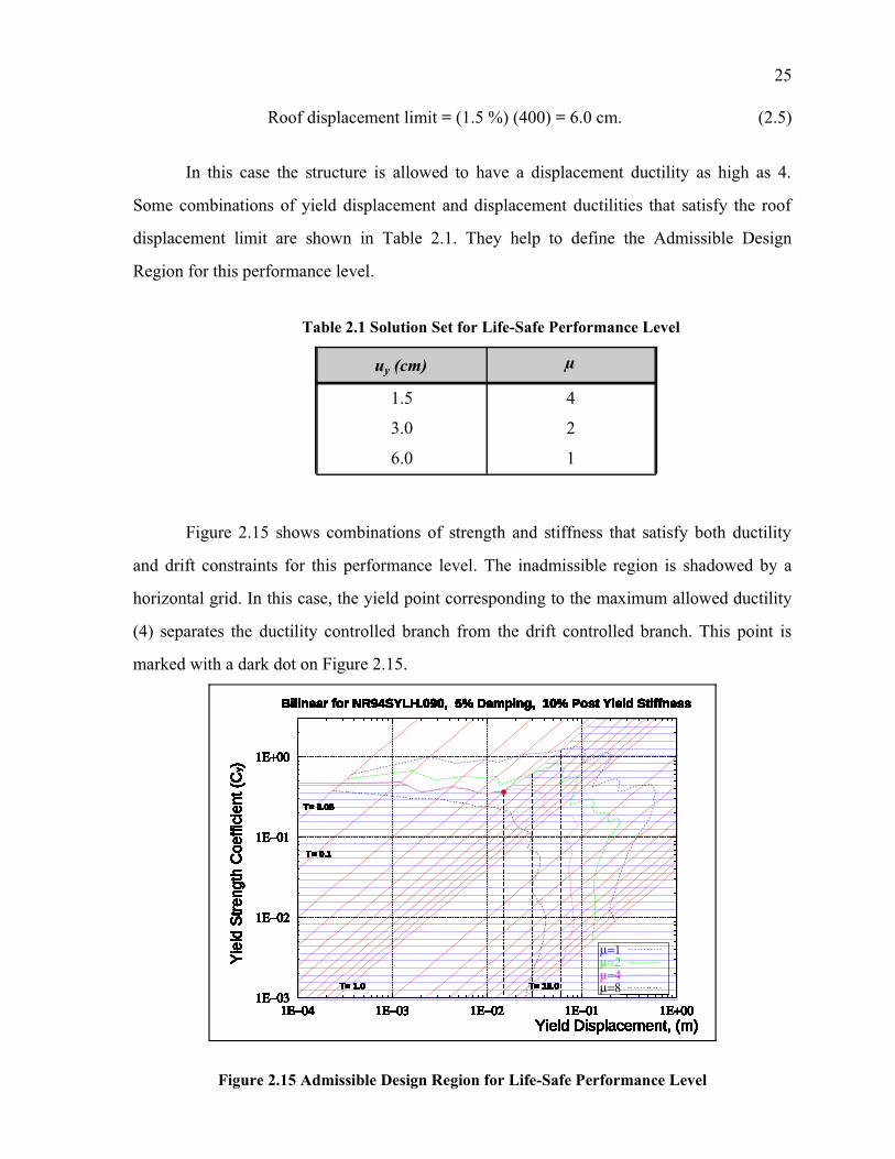
25
Roof displacement limit = (1.5 %) (400) = 6.0 cm. (2.5)
In this case the structure is allowed to have a displacement ductility as high as 4.
Some combinations of yield displacement and displacement ductilities that satisfy the roof
displacement limit are shown in Table 2.1. They help to define the Admissible Design
Region for this performance level.
Figure 2.15 shows combinations of strength and stiffness that satisfy both ductility
and drift constraints for this performance level. The inadmissible region is shadowed by a
horizontal grid. In this case, the yield point corresponding to the maximum allowed ductility
(4) separates the ductility controlled branch from the drift controlled branch. This point is
marked with a dark dot on Figure 2.15.
Figure 2.15 Admissible Design Region for Life-Safe Performance Level
1Ε−03
1Ε−02
1Ε−01
1Ε+00
1Ε−04 1Ε−03 1Ε−02 1Ε−01 1Ε+00
Bilinear for NR94SYLH.090, 5% Damping, 10% Post Yield Stiffness
Yie
ld S
tren
gth
Coe
ffici
ent (
C )y
Yield Displacement, (m)
T= 0.05
T= 0.1
T= 1.0 T= 10.0
µ=1µ=2µ=4µ=8
1Ε−03
1Ε−02
1Ε−01
1Ε+00
1Ε−04 1Ε−03 1Ε−02 1Ε−01 1Ε+00
Bilinear for NR94SYLH.090, 5% Damping, 10% Post Yield Stiffness
Yie
ld S
tren
gth
Coe
ffici
ent (
C )y
Yield Displacement, (m)
T= 0.05
T= 0.1
T= 1.0 T= 10.01Ε−03
1Ε−02
1Ε−01
1Ε+00
1Ε−04 1Ε−03 1Ε−02 1Ε−01 1Ε+00
Bilinear for NR94SYLH.090, 5% Damping, 10% Post Yield Stiffness
Yie
ld S
tren
gth
Coe
ffici
ent (
C )y
Yield Displacement, (m)
T= 0.05
T= 0.1
T= 1.0 T= 10.01Ε−03
1Ε−02
1Ε−01
1Ε+00
1Ε−04 1Ε−03 1Ε−02 1Ε−01 1Ε+00
Bilinear for NR94SYLH.090, 5% Damping, 10% Post Yield Stiffness
Yie
ld S
tren
gth
Coe
ffici
ent (
C )y
Yield Displacement, (m)
T= 0.05
T= 0.1
T= 1.0 T= 10.01Ε−03
1Ε−02
1Ε−01
1Ε+00
1Ε−04 1Ε−03 1Ε−02 1Ε−01 1Ε+00
Bilinear for NR94SYLH.090, 5% Damping, 10% Post Yield Stiffness
Yie
ld S
tren
gth
Coe
ffici
ent (
C )y
Yield Displacement, (m)
T= 0.05
T= 0.1
T= 1.0 T= 10.01Ε−03
1Ε−02
1Ε−01
1Ε+00
1Ε−04 1Ε−03 1Ε−02 1Ε−01 1Ε+00
Bilinear for NR94SYLH.090, 5% Damping, 10% Post Yield Stiffness
Yie
ld S
tren
gth
Coe
ffici
ent (
C )y
Yield Displacement, (m)
T= 0.05
T= 0.1
T= 1.0 T= 10.01Ε−03
1Ε−02
1Ε−01
1Ε+00
1Ε−04 1Ε−03 1Ε−02 1Ε−01 1Ε+00
Bilinear for NR94SYLH.090, 5% Damping, 10% Post Yield Stiffness
Yie
ld S
tren
gth
Coe
ffici
ent (
C )y
Yield Displacement, (m)
T= 0.05
T= 0.1
T= 1.0 T= 10.01Ε−03
1Ε−02
1Ε−01
1Ε+00
1Ε−04 1Ε−03 1Ε−02 1Ε−01 1Ε+00
Bilinear for NR94SYLH.090, 5% Damping, 10% Post Yield Stiffness
Yie
ld S
tren
gth
Coe
ffici
ent (
C )y
Yield Displacement, (m)
T= 0.05
T= 0.1
T= 1.0 T= 10.01Ε−03
1Ε−02
1Ε−01
1Ε+00
1Ε−04 1Ε−03 1Ε−02 1Ε−01 1Ε+00
Bilinear for NR94SYLH.090, 5% Damping, 10% Post Yield Stiffness
Yie
ld S
tren
gth
Coe
ffici
ent (
C )y
Yield Displacement, (m)
T= 0.05
T= 0.1
T= 1.0 T= 10.01Ε−03
1Ε−02
1Ε−01
1Ε+00
1Ε−04 1Ε−03 1Ε−02 1Ε−01 1Ε+00
Bilinear for NR94SYLH.090, 5% Damping, 10% Post Yield Stiffness
Yie
ld S
tren
gth
Coe
ffici
ent (
C )y
Yield Displacement, (m)
T= 0.05
T= 0.1
T= 1.0 T= 10.01Ε−03
1Ε−02
1Ε−01
1Ε+00
1Ε−04 1Ε−03 1Ε−02 1Ε−01 1Ε+00
Bilinear for NR94SYLH.090, 5% Damping, 10% Post Yield Stiffness
Yie
ld S
tren
gth
Coe
ffici
ent (
C )y
Yield Displacement, (m)
T= 0.05
T= 0.1
T= 1.0 T= 10.01Ε−03
1Ε−02
1Ε−01
1Ε+00
1Ε−04 1Ε−03 1Ε−02 1Ε−01 1Ε+00
Bilinear for NR94SYLH.090, 5% Damping, 10% Post Yield Stiffness
Yie
ld S
tren
gth
Coe
ffici
ent (
C )y
Yield Displacement, (m)
T= 0.05
T= 0.1
T= 1.0 T= 10.01Ε−03
1Ε−02
1Ε−01
1Ε+00
1Ε−04 1Ε−03 1Ε−02 1Ε−01 1Ε+00
Bilinear for NR94SYLH.090, 5% Damping, 10% Post Yield Stiffness
Yie
ld S
tren
gth
Coe
ffici
ent (
C )y
Yield Displacement, (m)
T= 0.05
T= 0.1
T= 1.0 T= 10.01Ε−03
1Ε−02
1Ε−01
1Ε+00
1Ε−04 1Ε−03 1Ε−02 1Ε−01 1Ε+00
Bilinear for NR94SYLH.090, 5% Damping, 10% Post Yield Stiffness
Yie
ld S
tren
gth
Coe
ffici
ent (
C )y
Yield Displacement, (m)
T= 0.05
T= 0.1
T= 1.0 T= 10.01Ε−03
1Ε−02
1Ε−01
1Ε+00
1Ε−04 1Ε−03 1Ε−02 1Ε−01 1Ε+00
Bilinear for NR94SYLH.090, 5% Damping, 10% Post Yield Stiffness
Yie
ld S
tren
gth
Coe
ffici
ent (
C )y
Yield Displacement, (m)
T= 0.05
T= 0.1
T= 1.0 T= 10.01Ε−03
1Ε−02
1Ε−01
1Ε+00
1Ε−04 1Ε−03 1Ε−02 1Ε−01 1Ε+00
Bilinear for NR94SYLH.090, 5% Damping, 10% Post Yield Stiffness
Yie
ld S
tren
gth
Coe
ffici
ent (
C )y
Yield Displacement, (m)
T= 0.05
T= 0.1
T= 1.0 T= 10.01Ε−03
1Ε−02
1Ε−01
1Ε+00
1Ε−04 1Ε−03 1Ε−02 1Ε−01 1Ε+00
Bilinear for NR94SYLH.090, 5% Damping, 10% Post Yield Stiffness
Yie
ld S
tren
gth
Coe
ffici
ent (
C )y
Yield Displacement, (m)
T= 0.05
T= 0.1
T= 1.0 T= 10.01Ε−03
1Ε−02
1Ε−01
1Ε+00
1Ε−04 1Ε−03 1Ε−02 1Ε−01 1Ε+00
Bilinear for NR94SYLH.090, 5% Damping, 10% Post Yield Stiffness
Yie
ld S
tren
gth
Coe
ffici
ent (
C )y
Yield Displacement, (m)
T= 0.05
T= 0.1
T= 1.0 T= 10.01Ε−03
1Ε−02
1Ε−01
1Ε+00
1Ε−04 1Ε−03 1Ε−02 1Ε−01 1Ε+00
Bilinear for NR94SYLH.090, 5% Damping, 10% Post Yield Stiffness
Yie
ld S
tren
gth
Coe
ffici
ent (
C )y
Yield Displacement, (m)
T= 0.05
T= 0.1
T= 1.0 T= 10.01Ε−03
1Ε−02
1Ε−01
1Ε+00
1Ε−04 1Ε−03 1Ε−02 1Ε−01 1Ε+00
Bilinear for NR94SYLH.090, 5% Damping, 10% Post Yield Stiffness
Yie
ld S
tren
gth
Coe
ffici
ent (
C )y
Yield Displacement, (m)
T= 0.05
T= 0.1
T= 1.0 T= 10.01Ε−03
1Ε−02
1Ε−01
1Ε+00
1Ε−04 1Ε−03 1Ε−02 1Ε−01 1Ε+00
Bilinear for NR94SYLH.090, 5% Damping, 10% Post Yield Stiffness
Yie
ld S
tren
gth
Coe
ffici
ent (
C )y
Yield Displacement, (m)
T= 0.05
T= 0.1
T= 1.0 T= 10.0
Table 2.1 Solution Set for Life-Safe Performance Level
uy (cm)
1.5 4
3.0 2
6.0 1
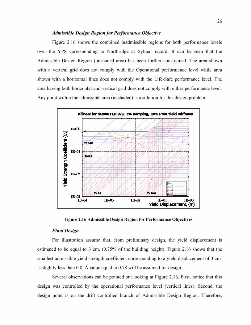
26
Admissible Design Region for Performance Objective
Figure 2.16 shows the combined inadmissible regions for both performance levels
over the YPS corresponding to Northridge at Sylmar record. It can be seen that the
Admissible Design Region (unshaded area) has been further constrained. The area shown
with a vertical grid does not comply with the Operational performance level while area
shown with a horizontal lines does not comply with the Life-Safe performance level. The
area having both horizontal and vertical grid does not comply with either performance level.
Any point within the admissible area (unshaded) is a solution for this design problem.
Final Design
For illustration assume that, from preliminary design, the yield displacement is
estimated to be equal to 3 cm. (0.75% of the building height). Figure 2.16 shows that the
smallest admissible yield strength coefficient corresponding to a yield displacement of 3 cm.
is slightly less than 0.8. A value equal to 0.78 will be assumed for design.
Several observations can be pointed out looking at Figure 2.16. First, notice that this
design was controlled by the operational performance level (vertical lines). Second, the
design point is on the drift controlled branch of Admissible Design Region. Therefore,
Figure 2.16 Admissible Design Region for Performance Objectives
1Ε−03
1Ε−02
1Ε−01
1Ε+00
1Ε−04 1Ε−03 1Ε−02 1Ε−01 1Ε+00
Bilinear for NR94SYLH.090, 5% Damping, 10% Post Yield Stiffness
Yie
ld S
tren
gth
Coe
ffici
ent (
C )y
Yield Displacement, (m)
T= 0.05
T= 0.1
T= 1.0 T= 10.0
µ=1µ=2µ=4µ=8
1Ε−03
1Ε−02
1Ε−01
1Ε+00
1Ε−04 1Ε−03 1Ε−02 1Ε−01 1Ε+00
Bilinear for NR94SYLH.090, 5% Damping, 10% Post Yield Stiffness
Yie
ld S
tren
gth
Coe
ffici
ent (
C )y
Yield Displacement, (m)
T= 0.05
T= 0.1
T= 1.0 T= 10.01Ε−03
1Ε−02
1Ε−01
1Ε+00
1Ε−04 1Ε−03 1Ε−02 1Ε−01 1Ε+00
Bilinear for NR94SYLH.090, 5% Damping, 10% Post Yield Stiffness
Yie
ld S
tren
gth
Coe
ffici
ent (
C )y
Yield Displacement, (m)
T= 0.05
T= 0.1
T= 1.0 T= 10.01Ε−03
1Ε−02
1Ε−01
1Ε+00
1Ε−04 1Ε−03 1Ε−02 1Ε−01 1Ε+00
Bilinear for NR94SYLH.090, 5% Damping, 10% Post Yield Stiffness
Yie
ld S
tren
gth
Coe
ffici
ent (
C )y
Yield Displacement, (m)
T= 0.05
T= 0.1
T= 1.0 T= 10.01Ε−03
1Ε−02
1Ε−01
1Ε+00
1Ε−04 1Ε−03 1Ε−02 1Ε−01 1Ε+00
Bilinear for NR94SYLH.090, 5% Damping, 10% Post Yield Stiffness
Yie
ld S
tren
gth
Coe
ffici
ent (
C )y
Yield Displacement, (m)
T= 0.05
T= 0.1
T= 1.0 T= 10.01Ε−03
1Ε−02
1Ε−01
1Ε+00
1Ε−04 1Ε−03 1Ε−02 1Ε−01 1Ε+00
Bilinear for NR94SYLH.090, 5% Damping, 10% Post Yield Stiffness
Yie
ld S
tren
gth
Coe
ffici
ent (
C )y
Yield Displacement, (m)
T= 0.05
T= 0.1
T= 1.0 T= 10.01Ε−03
1Ε−02
1Ε−01
1Ε+00
1Ε−04 1Ε−03 1Ε−02 1Ε−01 1Ε+00
Bilinear for NR94SYLH.090, 5% Damping, 10% Post Yield Stiffness
Yie
ld S
tren
gth
Coe
ffici
ent (
C )y
Yield Displacement, (m)
T= 0.05
T= 0.1
T= 1.0 T= 10.01Ε−03
1Ε−02
1Ε−01
1Ε+00
1Ε−04 1Ε−03 1Ε−02 1Ε−01 1Ε+00
Bilinear for NR94SYLH.090, 5% Damping, 10% Post Yield Stiffness
Yie
ld S
tren
gth
Coe
ffici
ent (
C )y
Yield Displacement, (m)
T= 0.05
T= 0.1
T= 1.0 T= 10.01Ε−03
1Ε−02
1Ε−01
1Ε+00
1Ε−04 1Ε−03 1Ε−02 1Ε−01 1Ε+00
Bilinear for NR94SYLH.090, 5% Damping, 10% Post Yield Stiffness
Yie
ld S
tren
gth
Coe
ffici
ent (
C )y
Yield Displacement, (m)
T= 0.05
T= 0.1
T= 1.0 T= 10.01Ε−03
1Ε−02
1Ε−01
1Ε+00
1Ε−04 1Ε−03 1Ε−02 1Ε−01 1Ε+00
Bilinear for NR94SYLH.090, 5% Damping, 10% Post Yield Stiffness
Yie
ld S
tren
gth
Coe
ffici
ent (
C )y
Yield Displacement, (m)
T= 0.05
T= 0.1
T= 1.0 T= 10.01Ε−03
1Ε−02
1Ε−01
1Ε+00
1Ε−04 1Ε−03 1Ε−02 1Ε−01 1Ε+00
Bilinear for NR94SYLH.090, 5% Damping, 10% Post Yield Stiffness
Yie
ld S
tren
gth
Coe
ffici
ent (
C )y
Yield Displacement, (m)
T= 0.05
T= 0.1
T= 1.0 T= 10.01Ε−03
1Ε−02
1Ε−01
1Ε+00
1Ε−04 1Ε−03 1Ε−02 1Ε−01 1Ε+00
Bilinear for NR94SYLH.090, 5% Damping, 10% Post Yield Stiffness
Yie
ld S
tren
gth
Coe
ffici
ent (
C )y
Yield Displacement, (m)
T= 0.05
T= 0.1
T= 1.0 T= 10.01Ε−03
1Ε−02
1Ε−01
1Ε+00
1Ε−04 1Ε−03 1Ε−02 1Ε−01 1Ε+00
Bilinear for NR94SYLH.090, 5% Damping, 10% Post Yield Stiffness
Yie
ld S
tren
gth
Coe
ffici
ent (
C )y
Yield Displacement, (m)
T= 0.05
T= 0.1
T= 1.0 T= 10.01Ε−03
1Ε−02
1Ε−01
1Ε+00
1Ε−04 1Ε−03 1Ε−02 1Ε−01 1Ε+00
Bilinear for NR94SYLH.090, 5% Damping, 10% Post Yield Stiffness
Yie
ld S
tren
gth
Coe
ffici
ent (
C )y
Yield Displacement, (m)
T= 0.05
T= 0.1
T= 1.0 T= 10.01Ε−03
1Ε−02
1Ε−01
1Ε+00
1Ε−04 1Ε−03 1Ε−02 1Ε−01 1Ε+00
Bilinear for NR94SYLH.090, 5% Damping, 10% Post Yield Stiffness
Yie
ld S
tren
gth
Coe
ffici
ent (
C )y
Yield Displacement, (m)
T= 0.05
T= 0.1
T= 1.0 T= 10.01Ε−03
1Ε−02
1Ε−01
1Ε+00
1Ε−04 1Ε−03 1Ε−02 1Ε−01 1Ε+00
Bilinear for NR94SYLH.090, 5% Damping, 10% Post Yield Stiffness
Yie
ld S
tren
gth
Coe
ffici
ent (
C )y
Yield Displacement, (m)
T= 0.05
T= 0.1
T= 1.0 T= 10.01Ε−03
1Ε−02
1Ε−01
1Ε+00
1Ε−04 1Ε−03 1Ε−02 1Ε−01 1Ε+00
Bilinear for NR94SYLH.090, 5% Damping, 10% Post Yield Stiffness
Yie
ld S
tren
gth
Coe
ffici
ent (
C )y
Yield Displacement, (m)
T= 0.05
T= 0.1
T= 1.0 T= 10.01Ε−03
1Ε−02
1Ε−01
1Ε+00
1Ε−04 1Ε−03 1Ε−02 1Ε−01 1Ε+00
Bilinear for NR94SYLH.090, 5% Damping, 10% Post Yield Stiffness
Yie
ld S
tren
gth
Coe
ffici
ent (
C )y
Yield Displacement, (m)
T= 0.05
T= 0.1
T= 1.0 T= 10.01Ε−03
1Ε−02
1Ε−01
1Ε+00
1Ε−04 1Ε−03 1Ε−02 1Ε−01 1Ε+00
Bilinear for NR94SYLH.090, 5% Damping, 10% Post Yield Stiffness
Yie
ld S
tren
gth
Coe
ffici
ent (
C )y
Yield Displacement, (m)
T= 0.05
T= 0.1
T= 1.0 T= 10.01Ε−03
1Ε−02
1Ε−01
1Ε+00
1Ε−04 1Ε−03 1Ε−02 1Ε−01 1Ε+00
Bilinear for NR94SYLH.090, 5% Damping, 10% Post Yield Stiffness
Yie
ld S
tren
gth
Coe
ffici
ent (
C )y
Yield Displacement, (m)
T= 0.05
T= 0.1
T= 1.0 T= 10.01Ε−03
1Ε−02
1Ε−01
1Ε+00
1Ε−04 1Ε−03 1Ε−02 1Ε−01 1Ε+00
Bilinear for NR94SYLH.090, 5% Damping, 10% Post Yield Stiffness
Yie
ld S
tren
gth
Coe
ffici
ent (
C )y
Yield Displacement, (m)
T= 0.05
T= 0.1
T= 1.0 T= 10.0

27
ductility demand will be less than the maximum allowed. Finally, observe that the design
point lies approximately over the 0.4 sec. period line.
The final structure will have the following characteristics:
Cy = 0.78 and uy = 0.03 m.
The required yield strength can be found using equation 2.1,
Vy = (Cy) (m) (g) = (0.78) (44) (9.807) = 337 kN. (2.6)
The period, obtained using equation 2.2, is 0.39 sec.
The final structure should have a peak displacement not larger than 2 cm (drift equal
to 0.5%) responding to the occasional earthquake, and not larger than 6 cm. (drift equal to
1.5%) under the action of the rare earthquake.
Figure 2.17 shows displacement response histories corresponding to the SDOF
building designed using Yield Point Spectra for the two performance levels. From the figure
it can be seen that both performance objectives (elastic response with peak displacement not
exceeding 2 cm. under Spitak at Gukasyan record, and no more than 6 cm. of displacement
under the Sylmar record) were satisfied.
Figure 2.17 Time History For Numerical Example 2
-2.00-1.50-1.00-0.500.000.501.001.502.00
0 5 10 15 20
Dis
plac
emen
t (cm
.)
Time (sec.)
Response to Gukasyan Record
-6.00
-4.00
-2.00
0.00
2.00
4.00
6.00
0 5 10 15 20
Response to Sylmar Record
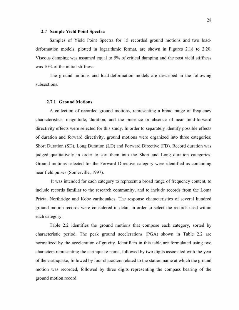
28
2.7 Sample Yield Point Spectra
Samples of Yield Point Spectra for 15 recorded ground motions and two load-
deformation models, plotted in logarithmic format, are shown in Figures 2.18 to 2.20.
Viscous damping was assumed equal to 5% of critical damping and the post yield stiffness
was 10% of the initial stiffness.
The ground motions and load-deformation models are described in the following
subsections.
2.7.1 Ground Motions
A collection of recorded ground motions, representing a broad range of frequency
characteristics, magnitude, duration, and the presence or absence of near field-forward
directivity effects were selected for this study. In order to separately identify possible effects
of duration and forward directivity, ground motions were organized into three categories;
Short Duration (SD), Long Duration (LD) and Forward Directive (FD). Record duration was
judged qualitatively in order to sort them into the Short and Long duration categories.
Ground motions selected for the Forward Directive category were identified as containing
near field pulses (Somerville, 1997).
It was intended for each category to represent a broad range of frequency content, to
include records familiar to the research community, and to include records from the Loma
Prieta, Northridge and Kobe earthquakes. The response characteristics of several hundred
ground motion records were considered in detail in order to select the records used within
each category.
Table 2.2 identifies the ground motions that compose each category, sorted by
characteristic period. The peak ground accelerations (PGA) shown in Table 2.2 are
normalized by the acceleration of gravity. Identifiers in this table are formulated using two
characters representing the earthquake name, followed by two digits associated with the year
of the earthquake, followed by four characters related to the station name at which the ground
motion was recorded, followed by three digits representing the compass bearing of the
ground motion record.

29
Figure 2.18 Yield Point Spectra for Short Duration Ground Motions
1Ε−03
1Ε−02
1Ε−01
1Ε+00
SHORT DURATION MOTIONSY
ield
Str
engt
h C
oeffi
cien
t (C
y)
Yield Displacement, (m)
Bilinear Stiffness Degrading
WN87MWLN.090
µ=1µ=2µ=4µ=8
SHORT DURATION MOTIONSY
ield
Str
engt
h C
oeffi
cien
t (C
y)
Yield Displacement, (m)
Bilinear Stiffness Degrading
WN87MWLN.090
µ=1µ=2µ=4µ=8
1Ε−03
1Ε−02
1Ε−01
1Ε+00
SHORT DURATION MOTIONSY
ield
Str
engt
h C
oeffi
cien
t (C
y)
Yield Displacement, (m)
Bilinear Stiffness Degrading
WN87MWLN.090
BB92CIVC.360
SHORT DURATION MOTIONSY
ield
Str
engt
h C
oeffi
cien
t (C
y)
Yield Displacement, (m)
Bilinear Stiffness Degrading
WN87MWLN.090
BB92CIVC.360
1Ε−03
1Ε−02
1Ε−01
1Ε+00
SHORT DURATION MOTIONSY
ield
Str
engt
h C
oeffi
cien
t (C
y)
Yield Displacement, (m)
Bilinear Stiffness Degrading
WN87MWLN.090
BB92CIVC.360
SP88GUKA.360
SHORT DURATION MOTIONSY
ield
Str
engt
h C
oeffi
cien
t (C
y)
Yield Displacement, (m)
Bilinear Stiffness Degrading
WN87MWLN.090
BB92CIVC.360
SP88GUKA.360
1Ε−03
1Ε−02
1Ε−01
1Ε+00
SHORT DURATION MOTIONSY
ield
Str
engt
h C
oeffi
cien
t (C
y)
Yield Displacement, (m)
Bilinear Stiffness Degrading
WN87MWLN.090
BB92CIVC.360
SP88GUKA.360
LP89CORR.090
SHORT DURATION MOTIONSY
ield
Str
engt
h C
oeffi
cien
t (C
y)
Yield Displacement, (m)
Bilinear Stiffness Degrading
WN87MWLN.090
BB92CIVC.360
SP88GUKA.360
LP89CORR.090
1Ε−03
1Ε−02
1Ε−01
1Ε+00
1Ε−04 1Ε−03 1Ε−02 1Ε−01
SHORT DURATION MOTIONSY
ield
Str
engt
h C
oeffi
cien
t (C
y)
Yield Displacement, (m)
Bilinear Stiffness Degrading
WN87MWLN.090
BB92CIVC.360
SP88GUKA.360
LP89CORR.090
NR94CENT.360
1Ε−04 1Ε−03 1Ε−02 1Ε−01 1Ε+00
SHORT DURATION MOTIONSY
ield
Str
engt
h C
oeffi
cien
t (C
y)
Yield Displacement, (m)
Bilinear Stiffness Degrading
WN87MWLN.090
BB92CIVC.360
SP88GUKA.360
LP89CORR.090
NR94CENT.360
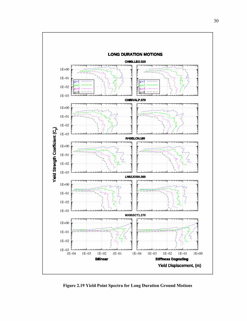
30
Figure 2.19 Yield Point Spectra for Long Duration Ground Motions
1Ε−03
1Ε−02
1Ε−01
1Ε+00
LONG DURATION MOTIONSY
ield
Str
engt
h C
oeffi
cien
t (C
y)
Yield Displacement, (m)
Bilinear Stiffness Degrading
CH85LLEO.010
µ=1µ=2µ=4µ=8
LONG DURATION MOTIONSY
ield
Str
engt
h C
oeffi
cien
t (C
y)
Yield Displacement, (m)
Bilinear Stiffness Degrading
CH85LLEO.010
µ=1µ=2µ=4µ=8
1Ε−03
1Ε−02
1Ε−01
1Ε+00
LONG DURATION MOTIONSY
ield
Str
engt
h C
oeffi
cien
t (C
y)
Yield Displacement, (m)
Bilinear Stiffness Degrading
CH85LLEO.010
CH85VALP.070
LONG DURATION MOTIONSY
ield
Str
engt
h C
oeffi
cien
t (C
y)
Yield Displacement, (m)
Bilinear Stiffness Degrading
CH85LLEO.010
CH85VALP.070
1Ε−03
1Ε−02
1Ε−01
1Ε+00
LONG DURATION MOTIONSY
ield
Str
engt
h C
oeffi
cien
t (C
y)
Yield Displacement, (m)
Bilinear Stiffness Degrading
CH85LLEO.010
CH85VALP.070
IV40ELCN.180
LONG DURATION MOTIONSY
ield
Str
engt
h C
oeffi
cien
t (C
y)
Yield Displacement, (m)
Bilinear Stiffness Degrading
CH85LLEO.010
CH85VALP.070
IV40ELCN.180
1Ε−03
1Ε−02
1Ε−01
1Ε+00
LONG DURATION MOTIONSY
ield
Str
engt
h C
oeffi
cien
t (C
y)
Yield Displacement, (m)
Bilinear Stiffness Degrading
CH85LLEO.010
CH85VALP.070
IV40ELCN.180
LN92JOSH.360
LONG DURATION MOTIONSY
ield
Str
engt
h C
oeffi
cien
t (C
y)
Yield Displacement, (m)
Bilinear Stiffness Degrading
CH85LLEO.010
CH85VALP.070
IV40ELCN.180
LN92JOSH.360
1Ε−03
1Ε−02
1Ε−01
1Ε+00
1Ε−04 1Ε−03 1Ε−02 1Ε−01
LONG DURATION MOTIONSY
ield
Str
engt
h C
oeffi
cien
t (C
y)
Yield Displacement, (m)
Bilinear Stiffness Degrading
CH85LLEO.010
CH85VALP.070
IV40ELCN.180
LN92JOSH.360
MX85SCT1.270
1Ε−04 1Ε−03 1Ε−02 1Ε−01 1Ε+00
LONG DURATION MOTIONSY
ield
Str
engt
h C
oeffi
cien
t (C
y)
Yield Displacement, (m)
Bilinear Stiffness Degrading
CH85LLEO.010
CH85VALP.070
IV40ELCN.180
LN92JOSH.360
MX85SCT1.270
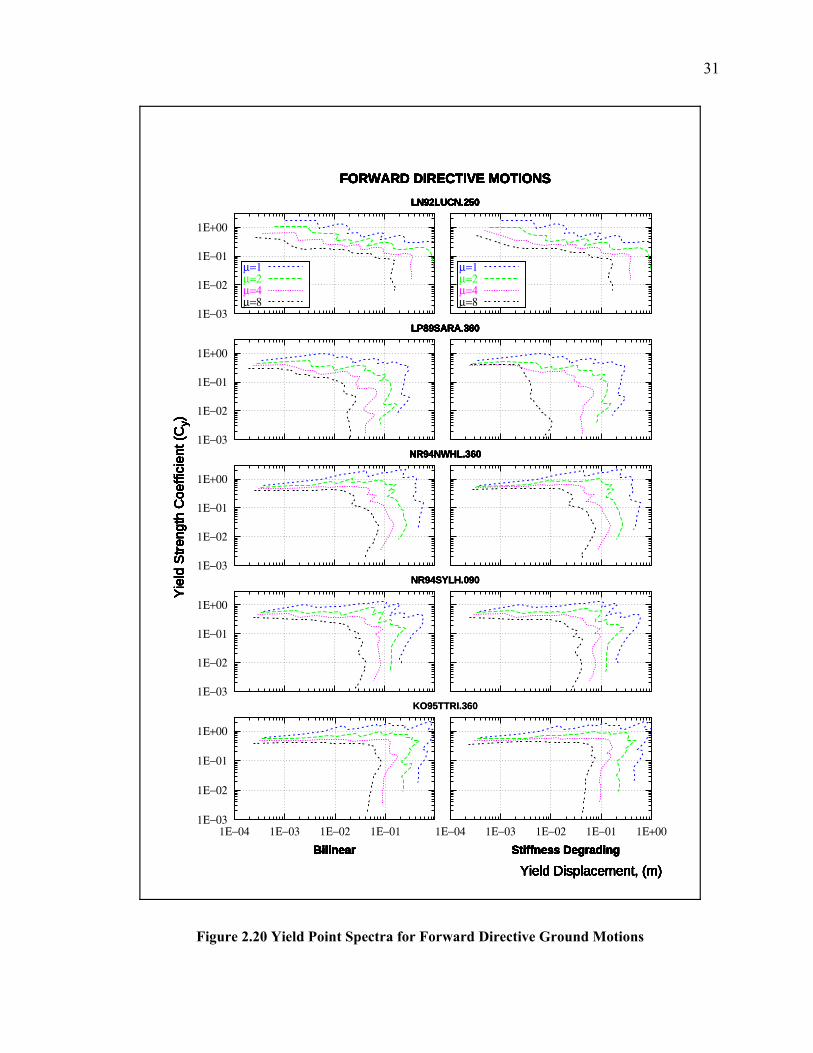
31
Figure 2.20 Yield Point Spectra for Forward Directive Ground Motions
1Ε−03
1Ε−02
1Ε−01
1Ε+00
FORWARD DIRECTIVE MOTIONSY
ield
Str
engt
h C
oeffi
cien
t (C
y)
Yield Displacement, (m)
Bilinear Stiffness Degrading
LN92LUCN.250
µ=1µ=2µ=4µ=8
FORWARD DIRECTIVE MOTIONSY
ield
Str
engt
h C
oeffi
cien
t (C
y)
Yield Displacement, (m)
Bilinear Stiffness Degrading
LN92LUCN.250
µ=1µ=2µ=4µ=8
1Ε−03
1Ε−02
1Ε−01
1Ε+00
FORWARD DIRECTIVE MOTIONSY
ield
Str
engt
h C
oeffi
cien
t (C
y)
Yield Displacement, (m)
Bilinear Stiffness Degrading
LN92LUCN.250
LP89SARA.360
FORWARD DIRECTIVE MOTIONSY
ield
Str
engt
h C
oeffi
cien
t (C
y)
Yield Displacement, (m)
Bilinear Stiffness Degrading
LN92LUCN.250
LP89SARA.360
1Ε−03
1Ε−02
1Ε−01
1Ε+00
FORWARD DIRECTIVE MOTIONSY
ield
Str
engt
h C
oeffi
cien
t (C
y)
Yield Displacement, (m)
Bilinear Stiffness Degrading
LN92LUCN.250
LP89SARA.360
NR94NWHL.360
FORWARD DIRECTIVE MOTIONSY
ield
Str
engt
h C
oeffi
cien
t (C
y)
Yield Displacement, (m)
Bilinear Stiffness Degrading
LN92LUCN.250
LP89SARA.360
NR94NWHL.360
1Ε−03
1Ε−02
1Ε−01
1Ε+00
FORWARD DIRECTIVE MOTIONSY
ield
Str
engt
h C
oeffi
cien
t (C
y)
Yield Displacement, (m)
Bilinear Stiffness Degrading
LN92LUCN.250
LP89SARA.360
NR94NWHL.360
NR94SYLH.090
FORWARD DIRECTIVE MOTIONSY
ield
Str
engt
h C
oeffi
cien
t (C
y)
Yield Displacement, (m)
Bilinear Stiffness Degrading
LN92LUCN.250
LP89SARA.360
NR94NWHL.360
NR94SYLH.090
1Ε−03
1Ε−02
1Ε−01
1Ε+00
1Ε−04 1Ε−03 1Ε−02 1Ε−01
FORWARD DIRECTIVE MOTIONSY
ield
Str
engt
h C
oeffi
cien
t (C
y)
Yield Displacement, (m)
Bilinear Stiffness Degrading
LN92LUCN.250
LP89SARA.360
NR94NWHL.360
NR94SYLH.090
KO95TTRI.360
1Ε−04 1Ε−03 1Ε−02 1Ε−01 1Ε+00
FORWARD DIRECTIVE MOTIONSY
ield
Str
engt
h C
oeffi
cien
t (C
y)
Yield Displacement, (m)
Bilinear Stiffness Degrading
LN92LUCN.250
LP89SARA.360
NR94NWHL.360
NR94SYLH.090
KO95TTRI.360

32
Various magnitude measures are reported in the literature and are repeated here for
reference: ML is the traditional local or Richter magnitude, Mw is moment magnitude, and MS
is the surface wave magnitude.
The characteristic period of each ground motion was established considering
equivalent velocity spectra and pseudo-acceleration spectra for linear elastic oscillators
having 5% damping. The equivalent velocity, Vm, is related to input energy, Em, and to
ground acceleration and velocity response by:
Table 2.2 Ground Motions Used for the Yield Point Spectra of Figures 2.18 to 2.20
Identifier Earthquake & Station Mag. Component
PGA/ g Char.Period (sec.)
Short Duration Motion (SD)
WN87MWLN.090 Whittier Narrows, at Mount Wilson ML = 6.1 90 0.175 0.20
BB92CIVC.360 Big Bear, at Civic Center MS = 6.6 360 0.544 0.40
SP88GUKA.360(*) Spitak, at Gukasyan-Armenia MS = 6.9 360 0.207 0.55
LP89CORR.090 Loma Prieta, at Corralitos MS = 7.1 90 0.478 0.85
NR94CENT.360 Northridge, at Century City MW = 6.6 360 0.221 1.20
Long Duration Motion (LD)
CH85LLEO.010 Central Chile, at Llolleo MS = 7.8 10 0.711 0.30
CH85VALP.070 Central Chile, at Valparaiso MS = 7.8 70 0.176 0.55
IV40ELCN.180 Imperial Valley, at El Centro ML = 6.3 180 0.348 0.65
LN92JOSH.360 Landers, at Joshua Tree MW = 7.5 360 0.274 1.30
MX85SCT1.270 Michoacan, at SCT1-Mexico City MS = 8.1 270 0.171 2.00
Forward Directive Motion (FD)
LN92LUCN.250(*) Landers, at Lucerne MW = 7.5 250 0.733 0.20
LP89SARA.360 Loma Prieta, at Saratoga ML = 6.6 315 0.504 0.35
NR94NWHL.360 Northridge, at Newhall MW = 6.7 360 0.589 0.80
NR94SYLH.090 Northridge, at Sylmar County MW = 6.7 90 0.604 0.90
KO95TTRI.360(*) Hyogo-Ken Nambu, at Takatori-kisu ML = 7.2 360 0.617 1.40
___________________
An asterisk (*) indicates that informal integration procedures were used to calculate the velocity anddisplacement histories in Figures A.1 through A15 contained in Appendix A

33
(2.7)
where: m is the mass of the oscillator,
is the ground acceleration, and
is the relative velocity of the oscillator mass.
The characteristic periods were identified using judgment to correspond
approximately to the first (lowest period) peak of the Equivalent Velocity Spectrum, and, at
the same time, the period at which the transition occurs between the constant acceleration
and constant velocity portions of a smooth design spectrum fitted to the 5% damped elastic
spectrum, following guidance given by Shimazaki (1984), Qi and Moehle (1991), and
Lepage (1997).
Detailed plots of the ground motions listed in Table 2.3 are presented in Appendix A.
2.7.2 Selected Load-Deformation Models
Two well known non-linear load-deformation models were used to construct the
Yield Point Spectra used throughout this research; the bilinear model and the stiffness-
degrading model. These load-deformation models are implemented in PCNSPEC
(Boroschek, 1991), and are described as follows.
• Bilinear Model. The bilinear model is defined by three parameters: yield strength, initial
stiffness and post-yield stiffness. Bilinear models are frequently used in modeling
structures that exhibit stable and full hysteretic loops.
• Stiffness Degrading Model. The stiffness degrading model is also defined by three
parameters: yield strength, initial stiffness, and post-yield stiffness. Just like the bilinear
model, the stiffness degrading model unloads with the initial elastic stiffness; however,
the stiffness degrading model softens when the force changes sign. After crossing the axis,
the model loads towards the previous point of maximum strength and displacement. The
stiffness degrading model is commonly used to represent reinforced concrete structures
that do not exhibit substantial degradation and/or bond deterioration.
12⋅m⋅V m
2 = Em = m∫ �xg �u dt
�x g
�u

34
Figure 2.21 shows the load-deformation response of two oscillators having a period
of vibration of 1.0 seconds to the 1940 N-S component of El Centro record. One plot
illustrate the bilinear model and the other illustrate the stiffness degrading model. The first
five seconds in the response of the oscillators are shown.
2.8 Summary
Yield Point Spectra (YPS), a type of Constant Ductility Response Spectra were
introduced. Their main characteristics and potential applications were described. Yield Point
Spectra for 15 ground motion records and two load-deformation models were presented.
Yield Point Spectra may be used in the analysis and design of SDOF systems. For
analysis YPS allow the peak displacement response and displacement ductility demand to be
estimated with good accuracy. In design applications, YPS permit the designer to determine
the strength and stiffness required to limit peak displacement and ductility demands to
arbitrary values. A detailed example describing the use of YPS in a performance-based
seismic design was included.
The idea of using the yield displacement of a structure instead of its period of
vibration as a key parameter to start seismic design was introduced.
Figure 2.21 Load-Deformation Relationship Used to Construct Yield Point Spectra
-0.20
-0.15
-0.10
-0.05
0.00
0.05
0.10
0.15
0.20
-10 -5 0 5 10
Yie
ld S
tren
gth
Coe
ffici
ent (
C )y
Displacement (cm.)
Bilinear Model
-0.20
-0.15
-0.10
-0.05
0.00
0.05
0.10
0.15
0.20
-10 -5 0 5 10
Yie
ld S
tren
gth
Coe
ffici
ent (
C )y
Displacement (cm.)
Stiffness Degrading Model

35
CHAPTER 3
EQUIVALENT SDOF MODEL OF MULTISTORY BUILDINGS
3.1 Introduction
The previous chapter discussed the representation of single-degree-of-freedom
(SDOF) systems using Yield Point Spectra (YPS). Yield Point Spectra were used to estimate
peak displacement response of SDOF systems and also to determine the strength and
stiffness needed to limit peak displacement response and ductility demands to arbitrary
values.
The peak displacement response of buildings under ground motion excitations,
ideally should be obtained using a nonlinear dynamic analysis of the whole structure. Even
though, for structures governed mainly by one mode of vibration, some investigators have
proposed that the response of multistory buildings can be approximated using an equivalent
SDOF system combined with an incremental nonlinear static analysis (pushover) as an
alternative to the more complex nonlinear dynamic analysis. This simplification is the basis
for methods such as the Displacement Coefficient Method and the Capacity Spectrum
Method, generally known as Nonlinear Static Procedures (NSPs).
The objective of this chapter is to provide a formulation that permits the use of Yield
Point Spectra for analysis and design of multistory buildings. Since Nonlinear Static
Procedures have used an equivalent single-degree-of-freedom modeling technique for a
similar objective, this technique is retained for use with Yield Point Spectra.
Buildings often are modeled as multi-degree-of-freedom (MDOF) systems in which
the distribution of mass, stiffness, and strength throughout the structure determines the
response of the various degrees of freedom to a base excitation. In this study, the degrees of
freedom considered for MDOF systems are the lateral displacements at each floor level in a
planar structure.
3.2 Equivalent Single-Degree-of-Freedom Modeling Technique
Representing the response of MDOF systems using an equivalent SDOF system has
been routinely used in the past and continues to be widely used. Over the last 40 years

36
numerous seismic codes have allowed buildings to be designed, either directly or indirectly,
using this technique. The methods proposed for design (Chapter 4) and analysis (Chapter 5)
of buildings using YPS rely upon the goodness of this technique.
The development of the equivalent SDOF modeling technique can be traced to the
early 60's (Biggs, 1964). Some later development can be found in the work by Saiidi and
Sozen (1981), and Qi and Moehle (1991). Most recently it has formed the basis for the
Nonlinear Static Procedures described in ATC-40 (1996) and in FEMA-273/274 (1997).
Even though various investigators have used different formulations for the technique,
all the formulations share two main assumptions. The first one postulates that response of the
MDOF system can be represented by a single deformed shape, while the second considers
that this deformed shape remains constant during the response.
Although it is known that both assumptions are not completely correct, the technique
has provided reasonable predictions of maximum displacement response of an MDOF
building, for structures when response is predominantly in the fundamental mode.
3.2.1 Displacement of Equivalent SDOF From MDOF Equation of Motion
The equivalent SDOF modeling technique describes the displacement response at
some representative point of a MDOF structure using an equivalent SDOF system. In this
work, as in ATC-40 and in FEMA-273/274, the representative point is taken at the top of the
MDOF system.
The best estimate of the displacement response of a multistory building is obtained by
solving the equation of motion for MDOF systems (Equation 3.1). Multistory buildings are
usually modeled as an MDOF system having mass lumped at each story level. For multistory
buildings responding elastically to a base excitation üg(t), the equation of motion can be
expressed as:
(3.1)
where: M is the diagonal mass matrix of the system,C is the damping matrix of the system,K is the stiffness matrix of the system,üg(t) is the ground acceleration history, andu(t) is the relative displacement vector of the MDOF system.
M {�u( t )}+C {�u( t )}+K {u( t )}=BM {1} �ug ( t )
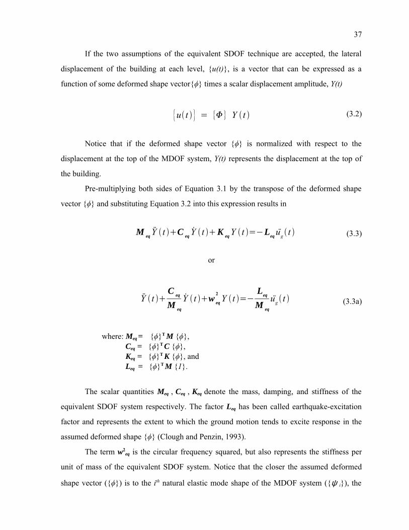
37
If the two assumptions of the equivalent SDOF technique are accepted, the lateral
displacement of the building at each level, {u(t)}, is a vector that can be expressed as a
function of some deformed shape vector{φ} times a scalar displacement amplitude, Y(t)
(3.2)
Notice that if the deformed shape vector {φ} is normalized with respect to the
displacement at the top of the MDOF system, Y(t) represents the displacement at the top of
the building.
Pre-multiplying both sides of Equation 3.1 by the transpose of the deformed shape
vector {φ} and substituting Equation 3.2 into this expression results in
(3.3)
or
(3.3a)
where: Meq = {φ}T M {φ}, Ceq = {φ}T C {φ}, Keq = {φ}T K {φ}, andLeq = {φ}T M {1}.
The scalar quantities Meq , Ceq , Keq denote the mass, damping, and stiffness of the
equivalent SDOF system respectively. The factor Leq has been called earthquake-excitation
factor and represents the extent to which the ground motion tends to excite response in the
assumed deformed shape {φ} (Clough and Penzin, 1993).
The term w2eq is the circular frequency squared, but also represents the stiffness per
unit of mass of the equivalent SDOF system. Notice that the closer the assumed deformed
shape vector ({φ}) is to the ith natural elastic mode shape of the MDOF system ({ψ i}), the
{u( t )} = {Φ} Y ( t )
M eq�Y ( t )+C eq
�Y ( t )+K eq Y ( t )=BLeq �ug ( t )
�Y ( t )+C eq
M eq
�Y ( t )+w eq
2Y ( t )=B
Leq
M eq
�ug ( t )

38
closer the circular frequency squared of the equivalent SDOF (w2eq) will be to the ith natural
circular frequency squared (w2i) of the MDOF system.
Equation 3.3a is the equation of motion of a unit mass SDOF system subjected to a
factored earthquake, where the factor, given by Leq/Meq, is generally known as the
participation factor. In this equation Y(t) still represents the displacement at the top of the
building provided that the deformed shape vector is normalized with respect to the top
displacement of the MDOF system.
Multiplying Equation 3.3a by Meq/Leq, a new displacement coordinate may be defined
as
(3.4)
and Equation 3.3a can be modified to
(3.5)
Equation 3.5 describes the displacement response of a unit mass SDOF system under
an unfactored earthquake. Here, usdof is the displacement of the equivalent SDOF, and the
product (weq2 usdof) is the force per unit of mass acting on the equivalent system.
Since, in general, Yield Point Spectra and others types of response spectra are usually
determined using unfactored ground motions, response displacements obtained from such
spectra correspond directly to solutions of Equation 3.5.
3.2.2 Yield Strength of the Equivalent SDOF System
The force per unit of mass acting on the equivalent system (weq2 usdof) can be used to
obtain the force acting on the equivalent SDOF at yield (its yield strength). For the instant
when the displacement of the equivalent SDOF system is equal to its yield displacement
(usdof = uysdof), the yield strength for a unit mass equivalent SDOF system can be expressed as
usdof( t ) =
M eq
Leq
Y ( t )
�usdof( t ) +
C eq
M eq
�usdof( t ) + w eq
2u
sdof( t ) = B �ug ( t )
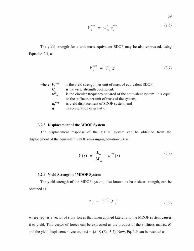
39
(3.6)
The yield strength for a unit mass equivalent SDOF may be also expressed, using
Equation 2.1, as
(3.7)
where: Vy sdof is the yield strength per unit of mass of equivalent SDOF,
Cy is the yield strength coefficient,
w2eq is the circular frequency squared of the equivalent system. It is equal
to the stiffness per unit of mass of the system,uy
sdof is yield displacement of SDOF system, andg is acceleration of gravity.
3.2.3 Displacement of the MDOF System
The displacement response of the MDOF system can be obtained from the
displacement of the equivalent SDOF rearranging equation 3.4 as
(3.8)
3.2.4 Yield Strength of MDOF System
The yield strength of the MDOF system, also known as base shear strength, can be
obtained as
(3.9)
where {Fy} is a vector of story forces that when applied laterally to the MDOF system causes
it to yield. This vector of forces can be expressed as the product of the stiffness matrix, K,
and the yield displacement vector, {uy} = {φ}Yy (Eq. 3.2). Now, Eq. 3.9 can be restated as
V y = {1}T⋅{F y }
V y
sdof= w eq
2⋅uy
sdof
V y
sdof= C y⋅g
Y ( t ) =Leq
M eq
⋅ usdof( t )

40
(3.10)
Here Yy is the displacement amplitude at the top of the MDOF system corresponding
to yield.
Replacing K with w2eq M, and substituting Equation 3.8 into Equation 3.10 gives
(3.11)
substituting Eq. 3.6 and Eq. 3.7 into Eq. 3.11
(3.12)
The quantity (Leq)2/ Meq has dimensions of mass and is sometimes called the effective
modal mass.
The ratio of the effective modal mass to the total mass of the building, is termed
effective modal mass coefficient, α,
(3.13)
where Mt is the total mass of the MDOF system.
Finally, the yield strength of the MDOF system can be expressed as
(3.14)
where Wt is the total weight of the building.
V y = {1}T⋅K⋅{φ}⋅Y y
V y = {1}T
M {φ}Leq
M eq
w eq
2uy
sdof=
Leq
2
M eq
w eq
2uy
sdof
V y =Leq
2
M eq
⋅C y⋅g
α =Leq
2
M eq⋅M t
V y = α ⋅C y⋅M t⋅g = α ⋅C y⋅W t

41
3.3 Application of the Equivalent SDOF Technique in Analysis and Design
The equivalent SDOF modeling technique can be applied to the analysis and design
of multistory buildings. It is particularly effective when response is dominated by a single
mode of deformation. Often this is the case for low and medium height buildings having
uniform mass and stiffness distributions. Therefore, it is reasonable to use an approximation
to the fundamental mode shape to apply the technique for analysis and design of this type of
buildings.
3.3.1 Selecting the Appropriate Deformed Shape Function {φ}
Under analysis situations, in which engineers want to check an existing design,
response simulations conducted in this study lead to recommend the first elastic mode shape
as the deformed shape to assume in applying the equivalent SDOF technique.
For design situations, where the exact elastic mode shapes can not yet be determined,
it is necessary to generate adequate shapes to apply the technique. Shapes having a
distribution of lateral deflections resembling the fundamental mode shape, for example,
inverted triangular or parabolic shapes, are generally sufficiently precise.
For many buildings, the distribution of mass is nearly uniform; then, the participation
factor (Leq/Meq), and the effective modal mass coefficient (α ) are functions of the deformed
mode shape {φ} only. Following Abrams (1985), these two parameters were determined for
three deformation shape functions: one triangular and two parabolic shapes, given by
formulas 3.15 to 3.17. The parabolic shapes represent reasonable bounds of likely shapes for
well-proportioned buildings.
(3.15)
(3.16)
(3.17)
{φ}={hi
H}
{φ}={1B(H Bhi)
2
H2 }
{φ}={hi
2
H2 }
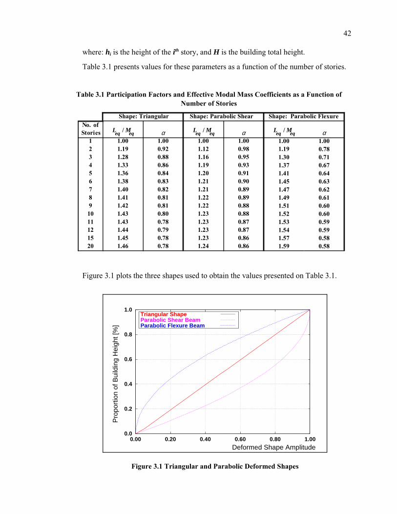
42
where: hi is the height of the ith story, and H is the building total height.
Table 3.1 presents values for these parameters as a function of the number of stories.
Figure 3.1 plots the three shapes used to obtain the values presented on Table 3.1.
Figure 3.1 Triangular and Parabolic Deformed Shapes
0.0
0.2
0.4
0.6
0.8
1.0
0.00 0.20 0.40 0.60 0.80 1.00
Pro
port
ion
of B
uild
ing
Hei
ght [
%]
Deformed Shape Amplitude
Triangular Shape Parabolic Shear Beam Parabolic Flexure Beam
Table 3.1 Participation Factors and Effective Modal Mass Coefficients as a Function ofNumber of Stories
Shape: Triangular Shape: Parabolic Shear Shape: Parabolic Flexure
α α α1 1.00 1.00 1.00 1.00 1.00 1.002 1.19 0.92 1.12 0.98 1.19 0.783 1.28 0.88 1.16 0.95 1.30 0.714 1.33 0.86 1.19 0.93 1.37 0.675 1.36 0.84 1.20 0.91 1.41 0.646 1.38 0.83 1.21 0.90 1.45 0.637 1.40 0.82 1.21 0.89 1.47 0.628 1.41 0.81 1.22 0.89 1.49 0.619 1.42 0.81 1.22 0.88 1.51 0.6010 1.43 0.80 1.23 0.88 1.52 0.6011 1.43 0.78 1.23 0.87 1.53 0.5912 1.44 0.79 1.23 0.87 1.54 0.5915 1.45 0.78 1.23 0.86 1.57 0.5820 1.46 0.78 1.24 0.86 1.59 0.58
N o . o f S t o r i e s Le q / Me q Le q / Me q Le q / Me q
43
3.4 Summary
A formulation that permits the use of Yield Point Spectra for the analysis and design
of multistory buildings was described. The formulation is based on the equivalent single-
degree-of freedom modeling technique.
The technique requires that an assumption be made with respect to the deformed
shape of the building. For analysis, it is recommended to assume the fundamental mode
shape of the building as the deformed shape to define the properties of the equivalent SDOF
system. For design, deformed shapes resembling the fundamental mode shape are generally
sufficiently precise.
Participation factors and modal mass coefficients were evaluated and tabulated for
three deformed shapes as function of the number of stories for the case in which the story
height and weight are uniform.

44
CHAPTER 4
DESIGN METHODOLOGY USING YIELD POINT SPECTRA
4.1 Introduction
Most seismic design codes in the U.S. and around the world allow structures to
undergo inelastic deformations in the event of the design earthquake. However, in most
practical situations, design is carried out using a set of equivalent static lateral forces in
conjunction with linear elastic analysis methods. Typically, explicit checks using inelastic
analysis are not required to determine the available strength and the ultimate deformation the
structure would experience responding to the design earthquake.
This chapter describes a methodology for the seismic design of regular multistory
buildings. The methodology is similar to the ones currently in use in the sense that a
minimum strength or design base shear force is determined for use in design. However, this
required minimum strength, which is obtained from Yield Point Spectra, is based on
constraints intended to directly limit the peak roof displacement of the building to user-
specified values. The objective of this limit imposed on the roof displacement is to try to
indirectly control interstory drift. Additionally this roof limit could also be used to control the
displacement ductility of the building. As in conventional seismic design methods, the design
base shear is vertically distributed over the height of the structure as a set of lateral forces.
This set of lateral forces is used for sizing structural members of the lateral force resisting
system, and also to estimate peak displacement and interstory drift indices.
The effectiveness of the Yield Point Spectra design methodology in limiting peak
displacement and system ductility demands is validated using numerical case study
examples. The case studies used to illustrate the proposed methodology consist of 4 moment-
resistant steel frames (two 4-story and two 12-story) designed to resist recorded strong
ground motions. Nonlinear static and dynamic analyses of each design were done to verify if
the proposed design methodology achieves the design objectives.
Although a procedure to select the members size and strength is not part of the
proposed methodology, in each of the examples a strong column-weak beam plastic hinge
mechanism was enforced through the selection of members sizes and strengths.

45
4.2 Design Philosophy
Structural deformation have been recognized as the centerpiece in evaluating
performance and damage state of structures (Algan, 1982). Under seismic excitations, this
performance is related to the displacement response of the structure. If satisfactory response
of the building under ground motions excitation is desired, displacement control of such
structures should be the main objective in earthquake resistant design (Qi and Moehle, 1991).
The idea of designing for displacement and checking strength rather than designing
for strength and checking displacement has been discussed before (Moehle, 1992). Even so,
the factor that has obstructed the adoption of displacement as the main parameter for seismic
design has been the difficulties involved in determining the maximum displacement that
develops during nonlinear response (Sozen and Lepage, 1996).
The objective of the design methodology introduced in this chapter is to limit the
maximum interstory drift index (IDI) of the multistory system, for a given intensity of
ground motion, to an arbitrary value. This objective is achieved indirectly, by establishing a
limit to the building's maximum roof displacement. The methodology mighty be easily
extended or modified to control the system displacement ductility demand, which in turn may
serve to indirectly control local ductility demands in the structure.
4.2.1 Design Premises
The design methodology combines the use of Yield Point Spectra with the equivalent
single degree of freedom formulation, presented in Chapter 3, for the design of multistory
systems. The methodology is based in the following premises: (1) the use of yield
displacement as an alternative to period as fundamental parameter for seismic design. (2) The
assumption that the nonlinear behavior of the multistory system is completely accounted for
in the SDOF responses represented in the YPS. Furthermore, the displacement ductility of
the building is assumed to be equal to the ductility of the equivalent SDOF system.
An implicit assumption inherent to the equivalent SDOF technique is also made here;
the deformed shape assumed to apply the equivalent SDOF formulation is a suitable
representation of the displacement profile of the multistory building responding to the design
ground motion.
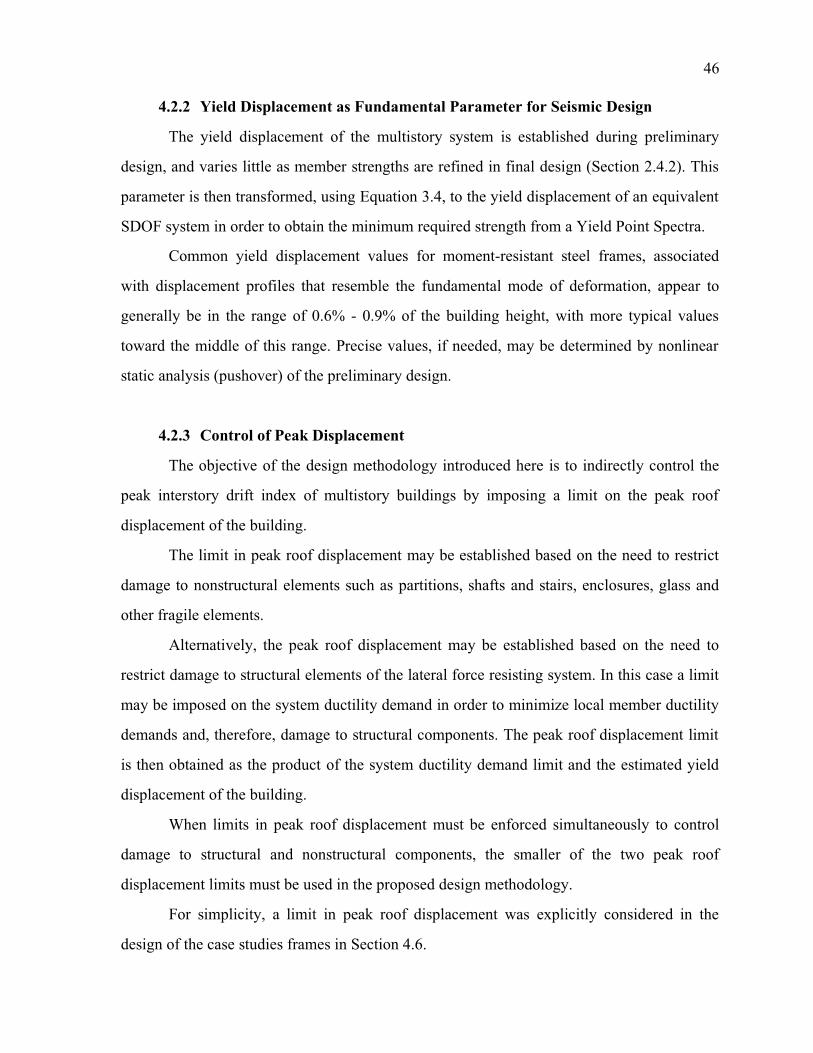
46
4.2.2 Yield Displacement as Fundamental Parameter for Seismic Design
The yield displacement of the multistory system is established during preliminary
design, and varies little as member strengths are refined in final design (Section 2.4.2). This
parameter is then transformed, using Equation 3.4, to the yield displacement of an equivalent
SDOF system in order to obtain the minimum required strength from a Yield Point Spectra.
Common yield displacement values for moment-resistant steel frames, associated
with displacement profiles that resemble the fundamental mode of deformation, appear to
generally be in the range of 0.6% - 0.9% of the building height, with more typical values
toward the middle of this range. Precise values, if needed, may be determined by nonlinear
static analysis (pushover) of the preliminary design.
4.2.3 Control of Peak Displacement
The objective of the design methodology introduced here is to indirectly control the
peak interstory drift index of multistory buildings by imposing a limit on the peak roof
displacement of the building.
The limit in peak roof displacement may be established based on the need to restrict
damage to nonstructural elements such as partitions, shafts and stairs, enclosures, glass and
other fragile elements.
Alternatively, the peak roof displacement may be established based on the need to
restrict damage to structural elements of the lateral force resisting system. In this case a limit
may be imposed on the system ductility demand in order to minimize local member ductility
demands and, therefore, damage to structural components. The peak roof displacement limit
is then obtained as the product of the system ductility demand limit and the estimated yield
displacement of the building.
When limits in peak roof displacement must be enforced simultaneously to control
damage to structural and nonstructural components, the smaller of the two peak roof
displacement limits must be used in the proposed design methodology.
For simplicity, a limit in peak roof displacement was explicitly considered in the
design of the case studies frames in Section 4.6.

47
4.2.4 Control of Interstory Drift Index as Final Design Objective
The interstory drift index (IDI) perhaps is the best parameter available to estimate the
damage a building would suffer after a strong ground motion. The interstory drift index is
defined as the displacement of any floor relative to the floor immediately below, normalized
by the story height. In this study, the imposition of a limit to the roof displacement is
considered to be an indirect way to limit interstory drift and, therefore, damage.
The roof drift index (peak displacement of the roof to the building height) is a
weighted average for all the interstory drift indices in a building. Generally, the peak
interstory drift index is larger than the roof drift index. Qi and Moehle (1991) report that the
interstory drift index can be as much as 30% larger than the roof drift index for reinforced
concrete structures. For moment-resistant steel frames, even larger values for the ratio of
interstory drift index and roof drift index have been reported; values as high as 1.4 (Collins,
1995) or even 2.0 (Krawinkler, 1997) have been observed in study analysis.
For the case studies developed in Section 4.6, the maximum roof displacement was
limited to 1.5% of the building height. The ratio of the peak interstory drift index to the roof
drift index was assumed as 1.5. Together, these two values were intended to limit the peak
interstory drift index to a value not larger than 2.25%. These values are used for illustration
purposes only; appropriate limits for use in design will depend on the design procedure, the
type of structural system, and the performance objectives.
4.2.5 Mixed Linear and Nonlinear Procedure
Since it is assumed that YPS account for the nonlinear behavior of the system, linear
static analysis can still be used to evaluate the building as designed. Peak roof displacement
and interstory drift indices are estimated multiplying results obtained from linear static
analysis by an estimated value of the system displacement ductility.
4.3 Limitations
The proposed design methodology applies to cases in which the equivalent SDOF
technique is applicable. Buildings should respond predominantly in a single mode and their
deformation profiles must reasonably match the deformed shape assumed in design.

48
Second Order (P-∆) effects are not explicitly addressed by the methodology, although
their influence in the response can be suppressed by limiting peak displacement response and
interstory drift to appropriate values.
The methodology is developed to address the strength of the lateral force resisting
system only and does not explicitly address design for gravity or wind loads.
4.4 Description of the YPS Design Methodology
In this section, a step by step description of the design methodology is outlined. The
procedure is illustrated and validated in Section 4.6, using some numerical examples. The
steps are as follow:
a) Based on the geometry of the structure, material properties, and preliminary
estimates of members depth, estimate the yield displacement (uy) of the structure
for a deformed profile similar to the fundamental mode of vibration. For many
moment resistant steel frames a value between 0.6% to 0.9% of the height of the
structure is reasonable.
b) Identify the desired peak roof displacement limit of the structure (uu). The value
should be selected to limit damage to tolerable amounts and could be associated
with a performance objective.
c) Estimate the allowable system displacement ductility demand of the building as
the ratio of the displacements obtained in steps a) and b) (æ = uu/uy).
d) Obtain the yield displacement of the equivalent SDOF system (uysdof) using
Equation 3.4. In this equation, the yield displacement for the building obtained in
step b) is used in place of the displacement amplitude, Y(t). Approximate values
for the participation factor (Leq/Meq), such as those presented in Table 3.1, appear
to be adequate for the design of regular buildings.
e) The yield displacement of the equivalent SDOF system, and the allowable system
ductility are used to determine the required yield strength coefficient (Cy) from the
Yield Point Spectrum associated with the design ground motion.

49
f) The required strength or design base shear (Vy) of the MDOF system is
determined using Equation 3.14. Approximate values for the effective modal mass
coefficient (α ), such as those presented in Table 3.1, appear to be adequate for
the design of regular buildings.
g) The design base shear is vertically distributed over the height of the structure to
obtain a set of lateral design forces. The base shear can be vertically distributed
over the height of the structure using familiar expressions such as the ones in the
Uniform Building Code (1997), reproduced here as Equations 4.1, 4.2 and 4.3.
The period of the equivalent SDOF can be used as an approximation to the
fundamental period of the building in Equation 4.3. This period can be obtained
using Equation 2.2. Observe that in the log-log format of the YPS, the parallel
lines represent constant period; thus, the approximate SDOF period may be read
directly from the YPS.
(4.1)
(4.2)
(4.3)
where: Ft is a concentrated force at the top of the building,Fi is the lateral force applied to each floor of the building, wj is the weight of floor j, hj is the interstory height of floor j, andT is the fundamental period of the building.
h) Members sizes and strengths should be selected following modern capacity design
methods and ductile detailing provisions recommendations. Strong column-weak
beam plastic hinge mechanism are suggested for good ductile behavior, although this
is not required. The following procedure was used to select structural members for all
V y = F t+∑i=1
n
F i
F i =(V
yBF
t)⋅w
i⋅h
i
(∑j= 1
n
wj⋅h
j)
F t = 0.07⋅T⋅V y

50
the frames of the case study examples. An initial set of members was selected using
the forces obtained in step g). Then, the selection was refined using the approximate
value of period (Equation 2.2) as a target to be matched by the first mode period of
the frame. A difference of ±5% between the actual and the approximate periods was
considered acceptable.1
i) Finally, linear static analysis is used to calculate the lateral displacements and
interstory drift indices for the designed structure. Peak roof displacement and
peak interstory drift indices are obtained by amplifying the linear results by the
estimated system displacement ductility obtained in step c). For a satisfactory
design, the peak linear estimates should be less than the desired limits.
4.5 Nonlinear Analysis for Verification Purposes
Static and dynamic nonlinear analyses were performed on the designed frames for
verification purposes. The computer program DRAIN-2DX (Powell et al., 1993) was used
for all the nonlinear analyses. A simple inelastic element (Element 02), capable of
developing plastic hinges, was located along the centerlines of the frames. Plastic hinge
strengths were assumed equal to the yield moments (Fy' S), with strain hardening equal to 5%
of Young's modulus. The yield strength of the steel was assumed as 248.0E+3 kN/m2 (36
ksi). Contribution of the floor slab, panel zones, action of gravity loads, and P-∆ effects were
not modeled.
Nonlinear static analyses (pushover) were used to confirm the actual values of yield
strength and yield displacement of the four frames considered. The pushover curves were
developed using a displacement control analysis with a displacement pattern proportional to
first mode shape.
Nonlinear dynamic analyses were done to compare the peak displacements and
interstory drifts developed in the nonlinear dynamic response to the linear estimates obtained
with the proposed methodology (step i). Recorded ground motions were used when
performing the nonlinear dynamic analysis verifications of each of the designed frames.
1 Other ways may be used to obtain the sizes and strengths of the members. In general, the procedure usedhere to size the members is not a component of the YPS design methodology.

51
4.6 Design Examples
The MDOF structures considered in this study consist of one set of two 4-story and
another set of two 12-story moment-resistant steel frames; all having three bays. The set of 4-
story frames are intended to represent low-height buildings while the set of 12-story
represents medium-height buildings.
The same performance level was used for the design of all the frames. The desired
performance level was to limit the peak roof displacement to 1.5% of the building height.
Because the ratio of the maximum expected interstory drift index to the roof drift index was
assumed to be 1.5, the peak interstory drift index in any story of the building is expected not
to exceed approximately 2.25% under the design ground motions.
The Yield Point Spectra used to design the frames correspond to ground motions that
were chosen among the 15 selected for this study (Section 2.7.1). It was desired to have one
flexible and one rigid design per set of buildings. For the 4-story buildings set, the ground
motions selected were the 250° component (perpendicular to strike) of the 1992 Landers at
Lucerne record for the flexible design, and the N-S component of the 1994 Northridge at
Newhall L.A. County Fire Station record for the rigid design. For the 12-story building set,
the E-W component of the 1985 Michoacan at Secretary of Communication and
Transportation (SCT1) and the N-S component of the 1995 Hyogo-Ken Nambu at Takatori-
kisu records were selected for the flexible and rigid designs respectively. The frames are
named Flexible-4, Rigid-4, Flexible-12 and Rigid-12 for reference.
All the frames were assumed to have an uniform mass distribution. The lower
columns were assumed fixed at the base level for all the frames considered. The lowest story
height was 5 m. and the remaining stories were 4 m. height; the columns were 8 m. on center.
4.6.1 Case Study 1: Design of Two 4-Story Buildings
4.6.1.1 Description of the 4-Story Moment-Resistant Frames
The general geometry for the 4-story buildings is shown in Figure 4.1. Story heights
and weights set are presented in Table 4.1. An uniform story weight of 551 kN was assumed,
for a total weight of 2204 kN. The total height of the frame is 17 m. Grade A36 steel was
used for all members.

52
Following the steps presented on Section 4.4 :
step a); limited data suggest that the yield displacement for a steel building, deformed
in a pattern similar to the fundamental mode, is often between 0.6 and 0.9% of the building
height. For this design, an initial estimate of 0.75% of the building height is assumed for the
yield displacement,
uy = (0.75%) (17 m) = 12.8 cm. (4.5)
Figure 4.1 Geometry of 4-Story Buildings
4.00 m.
4.00 m.
4.00 m.
5.00 m.
Fixed Column Bases
3 @ 8.00 m
Table 4.1 Story Heights and Weights of 4-Story Buildings
Story Height [m]4 4 5513 4 5512 4 5511 5 551
Total 17 2204
Weight [kN]

53
step b); a peak displacement limit of 1.5% of the building height is assumed,
therefore
uu = (1.5%) (17 m) = 25.5 cm. (4.6)
step c); given these values for the ultimate displacement (uu) and for the yield
displacement (uy), the system displacement ductility limit is
æ = uu/uy = 25.5/12.8 = 2 (4.7)
step d); the estimated yield displacement of the equivalent SDOF system is obtained
using Equation 3.4. For frames with uniformly-distributed masses, a triangular deformed
profile was used to apply the equivalent SDOF formulation. The value of the participation
factor (Leq/Meq) for the triangular shape, 1.33, is obtained from Table 3.1.
uysdof = 12.8/1.33 = 9.6 cm. (4.8)
Steps a) to d) are independent of the ground motion used for design. Now, steps e) to
i) are shown for each of the selected design ground motions.
4.6.1.2 Design of Flexible-4 Using the YPS for the Lucerne Ground Motion
step e); entering the YPS for the Lucerne ground motion with a yield displacement
equal to 9.6 cm. and a system displacement ductility limit of 2, the minimum acceptable yield
strength coefficient (Cy) is approximately to 0.3. This step is illustrated in Figure 4.2.
step f); the minimum required base shear or design yield strength (Vy) for the building
may be obtained using Equation 3.14. For the assumed triangular deformed shape, the
effective modal mass coefficient (α) is equal 0.86 (Table 3.1) resulting in
Vy = (0.86) (0.3) (2204) = 569 kN (4.9)

54
step g); the base shear obtained in step f), is vertically distributed using Equations 4.1
to 4.3. In order to use these equations, the designer must obtain an approximate value of the
fundamental period of the structure. This period may be obtained directly from Figure 4.2, in
which the lines of constant period plot as diagonal lines. Noting the logarithmic scale, the
period is observed to be between 1.1 and 1.2 sec.
Alternatively, Equation 2.2 may also be used:
(4.10)
Using Equation 4.3 to obtain the additional force applied to the top of the building,
Ft = (0.07) (1.13) (569) = 45 kN (4.11)
Applying Equation 4.2, the vertical distribution of the yield strength is found. The
lateral forces and the story shears are shown in Table 4.2.
Figure 4.2 Required Yield Strength Coefficient for the Flexible-4 Frame
1Ε−03
1Ε−02
1Ε−01
1Ε+00
1Ε−04 1Ε−03 1Ε−02 1Ε−01 1Ε+00
Bilinear for LN92LUCN.250, 5% Damping, 10% Post Yield Stiffness
Yie
ld S
tren
gth
Coe
ffici
ent (
C )y
Yield Displacement, (m)
T= 0.05
T= 0.1
T= 1.0 T= 10.0
µ=1µ=2µ=4µ=8
1Ε−03
1Ε−02
1Ε−01
1Ε+00
1Ε−04 1Ε−03 1Ε−02 1Ε−01 1Ε+00
Bilinear for LN92LUCN.250, 5% Damping, 10% Post Yield Stiffness
Yie
ld S
tren
gth
Coe
ffici
ent (
C )y
Yield Displacement, (m)
T= 0.05
T= 0.1
T= 1.0 T= 10.01Ε−03
1Ε−02
1Ε−01
1Ε+00
1Ε−04 1Ε−03 1Ε−02 1Ε−01 1Ε+00
Bilinear for LN92LUCN.250, 5% Damping, 10% Post Yield Stiffness
Yie
ld S
tren
gth
Coe
ffici
ent (
C )y
Yield Displacement, (m)
T= 0.05
T= 0.1
T= 1.0 T= 10.01Ε−03
1Ε−02
1Ε−01
1Ε+00
1Ε−04 1Ε−03 1Ε−02 1Ε−01 1Ε+00
Bilinear for LN92LUCN.250, 5% Damping, 10% Post Yield Stiffness
Yie
ld S
tren
gth
Coe
ffici
ent (
C )y
Yield Displacement, (m)
T= 0.05
T= 0.1
T= 1.0 T= 10.01Ε−03
1Ε−02
1Ε−01
1Ε+00
1Ε−04 1Ε−03 1Ε−02 1Ε−01 1Ε+00
Bilinear for LN92LUCN.250, 5% Damping, 10% Post Yield Stiffness
Yie
ld S
tren
gth
Coe
ffici
ent (
C )y
Yield Displacement, (m)
T= 0.05
T= 0.1
T= 1.0 T= 10.01Ε−03
1Ε−02
1Ε−01
1Ε+00
1Ε−04 1Ε−03 1Ε−02 1Ε−01 1Ε+00
Bilinear for LN92LUCN.250, 5% Damping, 10% Post Yield Stiffness
Yie
ld S
tren
gth
Coe
ffici
ent (
C )y
Yield Displacement, (m)
T= 0.05
T= 0.1
T= 1.0 T= 10.01Ε−03
1Ε−02
1Ε−01
1Ε+00
1Ε−04 1Ε−03 1Ε−02 1Ε−01 1Ε+00
Bilinear for LN92LUCN.250, 5% Damping, 10% Post Yield Stiffness
Yie
ld S
tren
gth
Coe
ffici
ent (
C )y
Yield Displacement, (m)
T= 0.05
T= 0.1
T= 1.0 T= 10.01Ε−03
1Ε−02
1Ε−01
1Ε+00
1Ε−04 1Ε−03 1Ε−02 1Ε−01 1Ε+00
Bilinear for LN92LUCN.250, 5% Damping, 10% Post Yield Stiffness
Yie
ld S
tren
gth
Coe
ffici
ent (
C )y
Yield Displacement, (m)
T= 0.05
T= 0.1
T= 1.0 T= 10.01Ε−03
1Ε−02
1Ε−01
1Ε+00
1Ε−04 1Ε−03 1Ε−02 1Ε−01 1Ε+00
Bilinear for LN92LUCN.250, 5% Damping, 10% Post Yield Stiffness
Yie
ld S
tren
gth
Coe
ffici
ent (
C )y
Yield Displacement, (m)
T= 0.05
T= 0.1
T= 1.0 T= 10.01Ε−03
1Ε−02
1Ε−01
1Ε+00
1Ε−04 1Ε−03 1Ε−02 1Ε−01 1Ε+00
Bilinear for LN92LUCN.250, 5% Damping, 10% Post Yield Stiffness
Yie
ld S
tren
gth
Coe
ffici
ent (
C )y
Yield Displacement, (m)
T= 0.05
T= 0.1
T= 1.0 T= 10.01Ε−03
1Ε−02
1Ε−01
1Ε+00
1Ε−04 1Ε−03 1Ε−02 1Ε−01 1Ε+00
Bilinear for LN92LUCN.250, 5% Damping, 10% Post Yield Stiffness
Yie
ld S
tren
gth
Coe
ffici
ent (
C )y
Yield Displacement, (m)
T= 0.05
T= 0.1
T= 1.0 T= 10.01Ε−03
1Ε−02
1Ε−01
1Ε+00
1Ε−04 1Ε−03 1Ε−02 1Ε−01 1Ε+00
Bilinear for LN92LUCN.250, 5% Damping, 10% Post Yield Stiffness
Yie
ld S
tren
gth
Coe
ffici
ent (
C )y
Yield Displacement, (m)
T= 0.05
T= 0.1
T= 1.0 T= 10.01Ε−03
1Ε−02
1Ε−01
1Ε+00
1Ε−04 1Ε−03 1Ε−02 1Ε−01 1Ε+00
Bilinear for LN92LUCN.250, 5% Damping, 10% Post Yield Stiffness
Yie
ld S
tren
gth
Coe
ffici
ent (
C )y
Yield Displacement, (m)
T= 0.05
T= 0.1
T= 1.0 T= 10.01Ε−03
1Ε−02
1Ε−01
1Ε+00
1Ε−04 1Ε−03 1Ε−02 1Ε−01 1Ε+00
Bilinear for LN92LUCN.250, 5% Damping, 10% Post Yield Stiffness
Yie
ld S
tren
gth
Coe
ffici
ent (
C )y
Yield Displacement, (m)
T= 0.05
T= 0.1
T= 1.0 T= 10.01Ε−03
1Ε−02
1Ε−01
1Ε+00
1Ε−04 1Ε−03 1Ε−02 1Ε−01 1Ε+00
Bilinear for LN92LUCN.250, 5% Damping, 10% Post Yield Stiffness
Yie
ld S
tren
gth
Coe
ffici
ent (
C )y
Yield Displacement, (m)
T= 0.05
T= 0.1
T= 1.0 T= 10.01Ε−03
1Ε−02
1Ε−01
1Ε+00
1Ε−04 1Ε−03 1Ε−02 1Ε−01 1Ε+00
Bilinear for LN92LUCN.250, 5% Damping, 10% Post Yield Stiffness
Yie
ld S
tren
gth
Coe
ffici
ent (
C )y
Yield Displacement, (m)
T= 0.05
T= 0.1
T= 1.0 T= 10.01Ε−03
1Ε−02
1Ε−01
1Ε+00
1Ε−04 1Ε−03 1Ε−02 1Ε−01 1Ε+00
Bilinear for LN92LUCN.250, 5% Damping, 10% Post Yield Stiffness
Yie
ld S
tren
gth
Coe
ffici
ent (
C )y
Yield Displacement, (m)
T= 0.05
T= 0.1
T= 1.0 T= 10.01Ε−03
1Ε−02
1Ε−01
1Ε+00
1Ε−04 1Ε−03 1Ε−02 1Ε−01 1Ε+00
Bilinear for LN92LUCN.250, 5% Damping, 10% Post Yield Stiffness
Yie
ld S
tren
gth
Coe
ffici
ent (
C )y
Yield Displacement, (m)
T= 0.05
T= 0.1
T= 1.0 T= 10.01Ε−03
1Ε−02
1Ε−01
1Ε+00
1Ε−04 1Ε−03 1Ε−02 1Ε−01 1Ε+00
Bilinear for LN92LUCN.250, 5% Damping, 10% Post Yield Stiffness
Yie
ld S
tren
gth
Coe
ffici
ent (
C )y
Yield Displacement, (m)
T= 0.05
T= 0.1
T= 1.0 T= 10.01Ε−03
1Ε−02
1Ε−01
1Ε+00
1Ε−04 1Ε−03 1Ε−02 1Ε−01 1Ε+00
Bilinear for LN92LUCN.250, 5% Damping, 10% Post Yield Stiffness
Yie
ld S
tren
gth
Coe
ffici
ent (
C )y
Yield Displacement, (m)
T= 0.05
T= 0.1
T= 1.0 T= 10.01Ε−03
1Ε−02
1Ε−01
1Ε+00
1Ε−04 1Ε−03 1Ε−02 1Ε−01 1Ε+00
Bilinear for LN92LUCN.250, 5% Damping, 10% Post Yield Stiffness
Yie
ld S
tren
gth
Coe
ffici
ent (
C )y
Yield Displacement, (m)
T= 0.05
T= 0.1
T= 1.0 T= 10.0
T = 2⋅π⋅9.6
0.3⋅980.7= 1.13 sec.

55
step h); the remaining design task is to select an appropriate set of members to
provide the required strength and stiffness to the frame. Figure 4.3 presents a set of Grade
A36 steel members that complies with the imposed strength and stiffness requirements. The
only constraint imposed in selecting the structural members was given for the enforcement of
a strong column-weak beam plastic mechanism; at each node, the summation of the strength
of the columns exceeds those of the beams at least by 20%. This constraint was enforced
only as a recommended practice, but is not essential to the proposed YPS design
methodology. The fundamental period for the frame shown in Figure 4.3 is 1.16 sec.
Table 4.2 Design Lateral Forces and Story Shears for the Flexible-4 Frame
Story4 247 2473 155 4022 107 5091 60 569
Force [kN] Shear [kN]
Figure 4.3 Flexible-4 Frame
T1 = 1.16 sec.
3 @ 8.00 m.
4.00 m.
4.00 m.
4.00 m.
5.00 m.
W21X44 W21X44W21X44
W21X44 W21X44W21X44
W21X44 W21X44W21X44
W21X44 W21X44W21X44
W14X74 W14X74 W14X74 W14X74
W14X48 W14X48 W14X48 W14X48
W14X48 W14X48 W14X48 W14X48
W14X74 W14X74 W14X74 W14X74
W14X74 W14X74 W14X74 W14X74
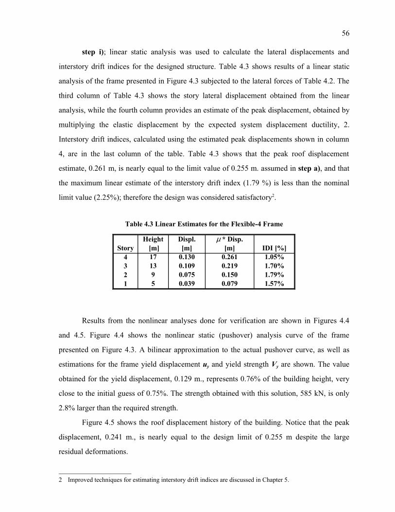
56
step i); linear static analysis was used to calculate the lateral displacements and
interstory drift indices for the designed structure. Table 4.3 shows results of a linear static
analysis of the frame presented in Figure 4.3 subjected to the lateral forces of Table 4.2. The
third column of Table 4.3 shows the story lateral displacement obtained from the linear
analysis, while the fourth column provides an estimate of the peak displacement, obtained by
multiplying the elastic displacement by the expected system displacement ductility, 2.
Interstory drift indices, calculated using the estimated peak displacements shown in column
4, are in the last column of the table. Table 4.3 shows that the peak roof displacement
estimate, 0.261 m, is nearly equal to the limit value of 0.255 m. assumed in step a), and that
the maximum linear estimate of the interstory drift index (1.79 %) is less than the nominal
limit value (2.25%); therefore the design was considered satisfactory2.
Results from the nonlinear analyses done for verification are shown in Figures 4.4
and 4.5. Figure 4.4 shows the nonlinear static (pushover) analysis curve of the frame
presented on Figure 4.3. A bilinear approximation to the actual pushover curve, as well as
estimations for the frame yield displacement uy and yield strength Vy are shown. The value
obtained for the yield displacement, 0.129 m., represents 0.76% of the building height, very
close to the initial guess of 0.75%. The strength obtained with this solution, 585 kN, is only
2.8% larger than the required strength.
Figure 4.5 shows the roof displacement history of the building. Notice that the peak
displacement, 0.241 m., is nearly equal to the design limit of 0.255 m despite the large
residual deformations.
2 Improved techniques for estimating interstory drift indices are discussed in Chapter 5.
Table 4.3 Linear Estimates for the Flexible-4 Frame
Story IDI [%]4 17 0.130 0.261 1.05%3 13 0.109 0.219 1.70%2 9 0.075 0.150 1.79%1 5 0.039 0.079 1.57%
Height [m]
Displ.[m]
µ * Disp.[m]

57
Figure 4.4 Nonlinear Static Analysis of the Flexible-4 Frame
0
100
200
300
400
500
600
700
0.00 0.05 0.10 0.15 0.20 0.25 0.30
Flexible-4 Frame
Bas
e S
hear
(kN
)
Roof Displacement, (m)
0.129 m
585 kN
1st Mode Pushover
Figure 4.5 Roof Displacement from Nonlinear Dynamic Analysis of the Flexible-4 Frame
-0.25
-0.20
-0.15
-0.10
-0.05
0.00
0.05
0.10
0.15
0.20
0.25
0 5 10 15 20 25 30 35 40 45 50
Flexible-4 Frame
Roo
f Dis
plac
emen
t (m
)
Time (sec)
Maximum Displacement = 0.241 m.
Design Record: Lucerne

58
Table 4.4 presents values of interstory drift index (IDI) obtained from nonlinear
dynamic analysis of this frame subjected to the Landers at Lucerne record. Peak values and
their timing are presented for each story. Notice that the nonlinear interstory drift index can
be larger than its linear equivalent in some stories. Observe that the nonlinear IDI for the
lowest story slightly exceed the nominal limit of 2.25%.
4.6.1.3 Design of Rigid-4 Using the YPS for the Newhall Ground Motion
The design continues from step d) of Section 4.6.1.1.
step e); entering the YPS for the Newhall ground motion, Figure 4.6, with the yield
displacement of 9.6 cm. and a system displacement ductility limit of 2, the minimum
acceptable yield strength coefficient (Cy) is equal to approximately 0.80. This step is
illustrated in Figure 4.6.
step f); the effective modal mass coefficient is the same used in the previous design.
The minimum required design yield strength (Vy) for the building is estimated using Equation
3.14 as
Vy = (0.86) (0.80) (2204) = 1516 kN (4.12)
step g); From Figure 4.6, the period is determined to be about 0.7 sec. Alternatively,
using Equation 2.2:
(4.13)
Table 4.4 Interstory Drift Indices from Nonlinear Dynamic Analysis of the Flexible-4
Story IDI [%] Time [Sec]4 0.60% 11.233 1.04% 11.262 1.85% 11.101 2.28% 11.07
T = 2⋅π⋅9.6
0.80⋅980.7= 0.70 sec.

59
Applying Equation 4.3, the additional force at the top of the building is
Ft = (0.07) (0.70) (1516) = 74 kN (4.14)
Using Equation 4.2, the final distribution of the base shear is found. The story forces
and shears are shown in Table 4.5.
Table 4.5 Design Lateral Forces and Story Shears for the Rigid-4 Frame
Figure 4.6 Required Yield Strength Coefficient for the Rigid-4 Frame
1Ε−03
1Ε−02
1Ε−01
1Ε+00
1Ε−04 1Ε−03 1Ε−02 1Ε−01 1Ε+00
Bilinear for NR94NWHL.360, 5% Damping, 10% Post Yield Stiffness
Yie
ld S
tren
gth
Coe
ffici
ent (
C )y
Yield Displacement, (m)
T= 0.05
T= 0.1
T= 1.0 T= 10.0
µ=1µ=2µ=4µ=8
1Ε−03
1Ε−02
1Ε−01
1Ε+00
1Ε−04 1Ε−03 1Ε−02 1Ε−01 1Ε+00
Bilinear for NR94NWHL.360, 5% Damping, 10% Post Yield Stiffness
Yie
ld S
tren
gth
Coe
ffici
ent (
C )y
Yield Displacement, (m)
T= 0.05
T= 0.1
T= 1.0 T= 10.01Ε−03
1Ε−02
1Ε−01
1Ε+00
1Ε−04 1Ε−03 1Ε−02 1Ε−01 1Ε+00
Bilinear for NR94NWHL.360, 5% Damping, 10% Post Yield Stiffness
Yie
ld S
tren
gth
Coe
ffici
ent (
C )y
Yield Displacement, (m)
T= 0.05
T= 0.1
T= 1.0 T= 10.01Ε−03
1Ε−02
1Ε−01
1Ε+00
1Ε−04 1Ε−03 1Ε−02 1Ε−01 1Ε+00
Bilinear for NR94NWHL.360, 5% Damping, 10% Post Yield Stiffness
Yie
ld S
tren
gth
Coe
ffici
ent (
C )y
Yield Displacement, (m)
T= 0.05
T= 0.1
T= 1.0 T= 10.01Ε−03
1Ε−02
1Ε−01
1Ε+00
1Ε−04 1Ε−03 1Ε−02 1Ε−01 1Ε+00
Bilinear for NR94NWHL.360, 5% Damping, 10% Post Yield Stiffness
Yie
ld S
tren
gth
Coe
ffici
ent (
C )y
Yield Displacement, (m)
T= 0.05
T= 0.1
T= 1.0 T= 10.01Ε−03
1Ε−02
1Ε−01
1Ε+00
1Ε−04 1Ε−03 1Ε−02 1Ε−01 1Ε+00
Bilinear for NR94NWHL.360, 5% Damping, 10% Post Yield Stiffness
Yie
ld S
tren
gth
Coe
ffici
ent (
C )y
Yield Displacement, (m)
T= 0.05
T= 0.1
T= 1.0 T= 10.01Ε−03
1Ε−02
1Ε−01
1Ε+00
1Ε−04 1Ε−03 1Ε−02 1Ε−01 1Ε+00
Bilinear for NR94NWHL.360, 5% Damping, 10% Post Yield Stiffness
Yie
ld S
tren
gth
Coe
ffici
ent (
C )y
Yield Displacement, (m)
T= 0.05
T= 0.1
T= 1.0 T= 10.01Ε−03
1Ε−02
1Ε−01
1Ε+00
1Ε−04 1Ε−03 1Ε−02 1Ε−01 1Ε+00
Bilinear for NR94NWHL.360, 5% Damping, 10% Post Yield Stiffness
Yie
ld S
tren
gth
Coe
ffici
ent (
C )y
Yield Displacement, (m)
T= 0.05
T= 0.1
T= 1.0 T= 10.01Ε−03
1Ε−02
1Ε−01
1Ε+00
1Ε−04 1Ε−03 1Ε−02 1Ε−01 1Ε+00
Bilinear for NR94NWHL.360, 5% Damping, 10% Post Yield Stiffness
Yie
ld S
tren
gth
Coe
ffici
ent (
C )y
Yield Displacement, (m)
T= 0.05
T= 0.1
T= 1.0 T= 10.01Ε−03
1Ε−02
1Ε−01
1Ε+00
1Ε−04 1Ε−03 1Ε−02 1Ε−01 1Ε+00
Bilinear for NR94NWHL.360, 5% Damping, 10% Post Yield Stiffness
Yie
ld S
tren
gth
Coe
ffici
ent (
C )y
Yield Displacement, (m)
T= 0.05
T= 0.1
T= 1.0 T= 10.01Ε−03
1Ε−02
1Ε−01
1Ε+00
1Ε−04 1Ε−03 1Ε−02 1Ε−01 1Ε+00
Bilinear for NR94NWHL.360, 5% Damping, 10% Post Yield Stiffness
Yie
ld S
tren
gth
Coe
ffici
ent (
C )y
Yield Displacement, (m)
T= 0.05
T= 0.1
T= 1.0 T= 10.01Ε−03
1Ε−02
1Ε−01
1Ε+00
1Ε−04 1Ε−03 1Ε−02 1Ε−01 1Ε+00
Bilinear for NR94NWHL.360, 5% Damping, 10% Post Yield Stiffness
Yie
ld S
tren
gth
Coe
ffici
ent (
C )y
Yield Displacement, (m)
T= 0.05
T= 0.1
T= 1.0 T= 10.01Ε−03
1Ε−02
1Ε−01
1Ε+00
1Ε−04 1Ε−03 1Ε−02 1Ε−01 1Ε+00
Bilinear for NR94NWHL.360, 5% Damping, 10% Post Yield Stiffness
Yie
ld S
tren
gth
Coe
ffici
ent (
C )y
Yield Displacement, (m)
T= 0.05
T= 0.1
T= 1.0 T= 10.01Ε−03
1Ε−02
1Ε−01
1Ε+00
1Ε−04 1Ε−03 1Ε−02 1Ε−01 1Ε+00
Bilinear for NR94NWHL.360, 5% Damping, 10% Post Yield Stiffness
Yie
ld S
tren
gth
Coe
ffici
ent (
C )y
Yield Displacement, (m)
T= 0.05
T= 0.1
T= 1.0 T= 10.01Ε−03
1Ε−02
1Ε−01
1Ε+00
1Ε−04 1Ε−03 1Ε−02 1Ε−01 1Ε+00
Bilinear for NR94NWHL.360, 5% Damping, 10% Post Yield Stiffness
Yie
ld S
tren
gth
Coe
ffici
ent (
C )y
Yield Displacement, (m)
T= 0.05
T= 0.1
T= 1.0 T= 10.01Ε−03
1Ε−02
1Ε−01
1Ε+00
1Ε−04 1Ε−03 1Ε−02 1Ε−01 1Ε+00
Bilinear for NR94NWHL.360, 5% Damping, 10% Post Yield Stiffness
Yie
ld S
tren
gth
Coe
ffici
ent (
C )y
Yield Displacement, (m)
T= 0.05
T= 0.1
T= 1.0 T= 10.01Ε−03
1Ε−02
1Ε−01
1Ε+00
1Ε−04 1Ε−03 1Ε−02 1Ε−01 1Ε+00
Bilinear for NR94NWHL.360, 5% Damping, 10% Post Yield Stiffness
Yie
ld S
tren
gth
Coe
ffici
ent (
C )y
Yield Displacement, (m)
T= 0.05
T= 0.1
T= 1.0 T= 10.01Ε−03
1Ε−02
1Ε−01
1Ε+00
1Ε−04 1Ε−03 1Ε−02 1Ε−01 1Ε+00
Bilinear for NR94NWHL.360, 5% Damping, 10% Post Yield Stiffness
Yie
ld S
tren
gth
Coe
ffici
ent (
C )y
Yield Displacement, (m)
T= 0.05
T= 0.1
T= 1.0 T= 10.01Ε−03
1Ε−02
1Ε−01
1Ε+00
1Ε−04 1Ε−03 1Ε−02 1Ε−01 1Ε+00
Bilinear for NR94NWHL.360, 5% Damping, 10% Post Yield Stiffness
Yie
ld S
tren
gth
Coe
ffici
ent (
C )y
Yield Displacement, (m)
T= 0.05
T= 0.1
T= 1.0 T= 10.01Ε−03
1Ε−02
1Ε−01
1Ε+00
1Ε−04 1Ε−03 1Ε−02 1Ε−01 1Ε+00
Bilinear for NR94NWHL.360, 5% Damping, 10% Post Yield Stiffness
Yie
ld S
tren
gth
Coe
ffici
ent (
C )y
Yield Displacement, (m)
T= 0.05
T= 0.1
T= 1.0 T= 10.01Ε−03
1Ε−02
1Ε−01
1Ε+00
1Ε−04 1Ε−03 1Ε−02 1Ε−01 1Ε+00
Bilinear for NR94NWHL.360, 5% Damping, 10% Post Yield Stiffness
Yie
ld S
tren
gth
Coe
ffici
ent (
C )y
Yield Displacement, (m)
T= 0.05
T= 0.1
T= 1.0 T= 10.0
Story4 631 6313 426 10572 295 13521 164 1516
Force [kN] Shear [kN]
60
step h); Figure 4.7 presents a set of Grade A36 steel members that complies with the
strength and stiffness requirements intended to limit roof drift to 1.5% of the frame height in
response to the Northridge at Newhall record. The fundamental period of this design is 0.71
sec.
step i); Table 4.6 presents the results of a linear static analysis of the frame of Figure
4.7 subjected to the lateral forces of Table 4.5. Table 4.6 shows that the peak roof
displacement estimate, 0.272 m., is slightly larger than the design limit of 0.255 m. in step
a). However, the estimated peak interstory drift index of 1.92 % is less than the limit value
2.25%.
Figure 4.7 Rigid-4 Frame
T1 = 0.71 Sec.
3 @ 8.00 m.
4.00 m.
4.00 m.
4.00 m.
5.00 m.
W24X55 W24X55W24X55
W14X99 W14X99 W14X99 W14X99
W14X99 W14X99 W14X99 W14X99
W14X176 W14X176 W14X176 W14X176
W24X55 W24X55W24X55
W24X94 W24X94W24X94
W24X94 W24X94W24X94
W14X176 W14X176 W14X176 W14X176

61
Results from the nonlinear analyses done for verification are shown in Figures 4.8
and 4.9. Figure 4.8 shows the nonlinear static (pushover) analysis curve of the frame
presented on Figure 4.7 A bilinear approximation of the actual pushover curve is also shown,
as well as estimates of the frame yield displacement uy and yield strength Vy. Notice that the
yield displacement, 0.133 m., represents 0.78% of the building height, close to the initial
estimate of 0.75% used in step b. The strength obtained with this solution, 1500 kN, is
98.9% of the estimated minimum required strength.
Table 4.6 Linear Estimates for the Rigid-4 Frame
Story IDI [%]4 17 0.136 0.272 1.42%3 13 0.108 0.215 1.92%2 9 0.069 0.138 1.62%1 5 0.037 0.074 1.47%
Height [m]
Displ.[m]
µ * Disp.[m]
Figure 4.8 Nonlinear Static Analysis of the Rigid-4 Frame
0
200
400
600
800
1000
1200
1400
1600
1800
0.00 0.05 0.10 0.15 0.20 0.25 0.30
Rigid-4 Frame
Bas
e S
hear
(kN
)
Roof Displacement, (m)
0.133 m
1500 kN
1st Mode Pushover

62
Figure 4.9 shows the roof displacement history of the frame. Observe that the actual
peak displacement of the roof, 0.223 m., is slightly less than the design limit for the roof
displacement of 0.255 m.
Table 4.7 presents values of the interstory drift index (IDI) obtained from nonlinear
dynamic analysis of the frame subjected to Newhall record. Peak values and their timing are
presented for each story. Although, the maximum interstory drifts shown in Table 4.7 differ
from the linear estimates in Table 4.6, for this case the interstory drifts in all stories were less
than the nominal limit value of 2.25%.
Figure 4.9 Roof Displacement from Nonlinear Dynamic Analysis of the Rigid-4 Frame
-0.25
-0.20
-0.15
-0.10
-0.05
0.00
0.05
0.10
0.15
0.20
0.25
0 5 10 15 20 25 30 35 40 45 50
Rigid-4 Frame
Roo
f Dis
plac
emen
t (m
)
Time (sec)
Maximum Displacement = 0.223 m.
Design Record: Newhall
Table 4.7 Interstory Drift Indices from Nonlinear Dynamic Analysis of the Rigid-4
Story IDI [%] Time [Sec]4 1.05% 5.703 1.42% 5.712 1.50% 5.401 1.64% 5.38
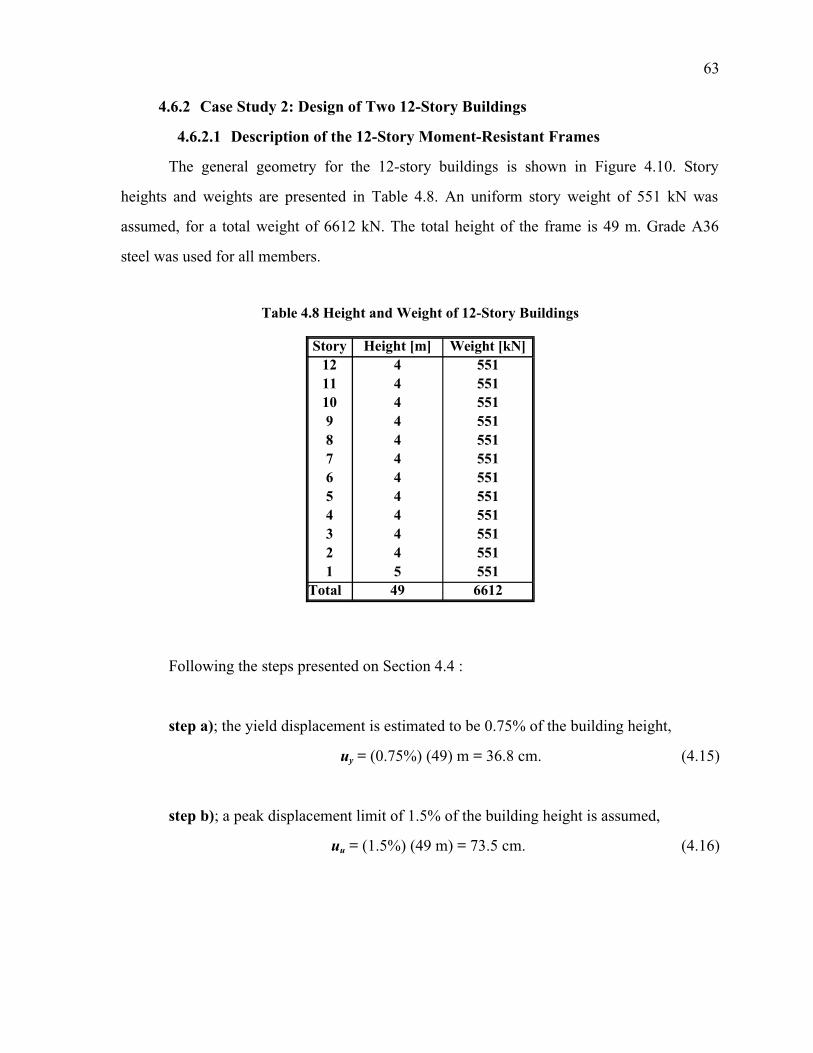
63
4.6.2 Case Study 2: Design of Two 12-Story Buildings
4.6.2.1 Description of the 12-Story Moment-Resistant Frames
The general geometry for the 12-story buildings is shown in Figure 4.10. Story
heights and weights are presented in Table 4.8. An uniform story weight of 551 kN was
assumed, for a total weight of 6612 kN. The total height of the frame is 49 m. Grade A36
steel was used for all members.
Following the steps presented on Section 4.4 :
step a); the yield displacement is estimated to be 0.75% of the building height,
uy = (0.75%) (49) m = 36.8 cm. (4.15)
step b); a peak displacement limit of 1.5% of the building height is assumed,
uu = (1.5%) (49 m) = 73.5 cm. (4.16)
Table 4.8 Height and Weight of 12-Story Buildings
Story Height [m]12 4 55111 4 55110 4 5519 4 5518 4 5517 4 5516 4 5515 4 5514 4 5513 4 5512 4 5511 5 551
Total 49 6612
Weight [kN]

64
Figure 4.10 Geometry of 12-Story Buildings
4.00 m
4.00 m
4.00 m
4.00 m
4.00 m
4.00 m
4.00 m
4.00 m
4.00 m
4.00 m
4.00 m
5.00 m
3 @ 8.00 m
Fixed Column Bases

65
step c); given these values for the ultimate displacement (uu) and for the yield
displacement (uy), the system displacement ductility limit is
æ = uu/uy = 73.5/36.8 = 2 (4.17)
step d); the yield displacement of the equivalent SDOF system is obtained using
Equation 3.4. Assuming a triangular deformed shape, the participation factor, Leq /Meq, for
this shape, 1.44, is obtained from Table 3.1.
uysdof = 36.8/1.44 = 26 cm. (4.18)
4.6.2.2 Design of Flexible-12 Using the YPS for the SCT1 Ground Motion
step e); entering the YPS for the SCT1 record with a yield displacement equal to 26
cm. and a system displacement ductility limit of 2, an acceptable yield strength coefficient
(Cy) is approximately 0.22. This step is illustrated in Figure 4.11.
Figure 4.11 Required Yield Strength Coefficient for the Flexible-12 Frame
1Ε−03
1Ε−02
1Ε−01
1Ε+00
1Ε−04 1Ε−03 1Ε−02 1Ε−01 1Ε+00
Bilinear for MX85SCT1.270, 5% Damping, 10% Post Yield Stiffness
Yie
ld S
tren
gth
Coe
ffici
ent (
C )y
Yield Displacement, (m)
T= 0.05
T= 0.1
T= 1.0 T= 10.0
µ=1µ=2µ=4µ=8
1Ε−03
1Ε−02
1Ε−01
1Ε+00
1Ε−04 1Ε−03 1Ε−02 1Ε−01 1Ε+00
Bilinear for MX85SCT1.270, 5% Damping, 10% Post Yield Stiffness
Yie
ld S
tren
gth
Coe
ffici
ent (
C )y
Yield Displacement, (m)
T= 0.05
T= 0.1
T= 1.0 T= 10.01Ε−03
1Ε−02
1Ε−01
1Ε+00
1Ε−04 1Ε−03 1Ε−02 1Ε−01 1Ε+00
Bilinear for MX85SCT1.270, 5% Damping, 10% Post Yield Stiffness
Yie
ld S
tren
gth
Coe
ffici
ent (
C )y
Yield Displacement, (m)
T= 0.05
T= 0.1
T= 1.0 T= 10.01Ε−03
1Ε−02
1Ε−01
1Ε+00
1Ε−04 1Ε−03 1Ε−02 1Ε−01 1Ε+00
Bilinear for MX85SCT1.270, 5% Damping, 10% Post Yield Stiffness
Yie
ld S
tren
gth
Coe
ffici
ent (
C )y
Yield Displacement, (m)
T= 0.05
T= 0.1
T= 1.0 T= 10.01Ε−03
1Ε−02
1Ε−01
1Ε+00
1Ε−04 1Ε−03 1Ε−02 1Ε−01 1Ε+00
Bilinear for MX85SCT1.270, 5% Damping, 10% Post Yield Stiffness
Yie
ld S
tren
gth
Coe
ffici
ent (
C )y
Yield Displacement, (m)
T= 0.05
T= 0.1
T= 1.0 T= 10.01Ε−03
1Ε−02
1Ε−01
1Ε+00
1Ε−04 1Ε−03 1Ε−02 1Ε−01 1Ε+00
Bilinear for MX85SCT1.270, 5% Damping, 10% Post Yield Stiffness
Yie
ld S
tren
gth
Coe
ffici
ent (
C )y
Yield Displacement, (m)
T= 0.05
T= 0.1
T= 1.0 T= 10.01Ε−03
1Ε−02
1Ε−01
1Ε+00
1Ε−04 1Ε−03 1Ε−02 1Ε−01 1Ε+00
Bilinear for MX85SCT1.270, 5% Damping, 10% Post Yield Stiffness
Yie
ld S
tren
gth
Coe
ffici
ent (
C )y
Yield Displacement, (m)
T= 0.05
T= 0.1
T= 1.0 T= 10.01Ε−03
1Ε−02
1Ε−01
1Ε+00
1Ε−04 1Ε−03 1Ε−02 1Ε−01 1Ε+00
Bilinear for MX85SCT1.270, 5% Damping, 10% Post Yield Stiffness
Yie
ld S
tren
gth
Coe
ffici
ent (
C )y
Yield Displacement, (m)
T= 0.05
T= 0.1
T= 1.0 T= 10.01Ε−03
1Ε−02
1Ε−01
1Ε+00
1Ε−04 1Ε−03 1Ε−02 1Ε−01 1Ε+00
Bilinear for MX85SCT1.270, 5% Damping, 10% Post Yield Stiffness
Yie
ld S
tren
gth
Coe
ffici
ent (
C )y
Yield Displacement, (m)
T= 0.05
T= 0.1
T= 1.0 T= 10.01Ε−03
1Ε−02
1Ε−01
1Ε+00
1Ε−04 1Ε−03 1Ε−02 1Ε−01 1Ε+00
Bilinear for MX85SCT1.270, 5% Damping, 10% Post Yield Stiffness
Yie
ld S
tren
gth
Coe
ffici
ent (
C )y
Yield Displacement, (m)
T= 0.05
T= 0.1
T= 1.0 T= 10.01Ε−03
1Ε−02
1Ε−01
1Ε+00
1Ε−04 1Ε−03 1Ε−02 1Ε−01 1Ε+00
Bilinear for MX85SCT1.270, 5% Damping, 10% Post Yield Stiffness
Yie
ld S
tren
gth
Coe
ffici
ent (
C )y
Yield Displacement, (m)
T= 0.05
T= 0.1
T= 1.0 T= 10.01Ε−03
1Ε−02
1Ε−01
1Ε+00
1Ε−04 1Ε−03 1Ε−02 1Ε−01 1Ε+00
Bilinear for MX85SCT1.270, 5% Damping, 10% Post Yield Stiffness
Yie
ld S
tren
gth
Coe
ffici
ent (
C )y
Yield Displacement, (m)
T= 0.05
T= 0.1
T= 1.0 T= 10.01Ε−03
1Ε−02
1Ε−01
1Ε+00
1Ε−04 1Ε−03 1Ε−02 1Ε−01 1Ε+00
Bilinear for MX85SCT1.270, 5% Damping, 10% Post Yield Stiffness
Yie
ld S
tren
gth
Coe
ffici
ent (
C )y
Yield Displacement, (m)
T= 0.05
T= 0.1
T= 1.0 T= 10.01Ε−03
1Ε−02
1Ε−01
1Ε+00
1Ε−04 1Ε−03 1Ε−02 1Ε−01 1Ε+00
Bilinear for MX85SCT1.270, 5% Damping, 10% Post Yield Stiffness
Yie
ld S
tren
gth
Coe
ffici
ent (
C )y
Yield Displacement, (m)
T= 0.05
T= 0.1
T= 1.0 T= 10.01Ε−03
1Ε−02
1Ε−01
1Ε+00
1Ε−04 1Ε−03 1Ε−02 1Ε−01 1Ε+00
Bilinear for MX85SCT1.270, 5% Damping, 10% Post Yield Stiffness
Yie
ld S
tren
gth
Coe
ffici
ent (
C )y
Yield Displacement, (m)
T= 0.05
T= 0.1
T= 1.0 T= 10.01Ε−03
1Ε−02
1Ε−01
1Ε+00
1Ε−04 1Ε−03 1Ε−02 1Ε−01 1Ε+00
Bilinear for MX85SCT1.270, 5% Damping, 10% Post Yield Stiffness
Yie
ld S
tren
gth
Coe
ffici
ent (
C )y
Yield Displacement, (m)
T= 0.05
T= 0.1
T= 1.0 T= 10.01Ε−03
1Ε−02
1Ε−01
1Ε+00
1Ε−04 1Ε−03 1Ε−02 1Ε−01 1Ε+00
Bilinear for MX85SCT1.270, 5% Damping, 10% Post Yield Stiffness
Yie
ld S
tren
gth
Coe
ffici
ent (
C )y
Yield Displacement, (m)
T= 0.05
T= 0.1
T= 1.0 T= 10.01Ε−03
1Ε−02
1Ε−01
1Ε+00
1Ε−04 1Ε−03 1Ε−02 1Ε−01 1Ε+00
Bilinear for MX85SCT1.270, 5% Damping, 10% Post Yield Stiffness
Yie
ld S
tren
gth
Coe
ffici
ent (
C )y
Yield Displacement, (m)
T= 0.05
T= 0.1
T= 1.0 T= 10.01Ε−03
1Ε−02
1Ε−01
1Ε+00
1Ε−04 1Ε−03 1Ε−02 1Ε−01 1Ε+00
Bilinear for MX85SCT1.270, 5% Damping, 10% Post Yield Stiffness
Yie
ld S
tren
gth
Coe
ffici
ent (
C )y
Yield Displacement, (m)
T= 0.05
T= 0.1
T= 1.0 T= 10.01Ε−03
1Ε−02
1Ε−01
1Ε+00
1Ε−04 1Ε−03 1Ε−02 1Ε−01 1Ε+00
Bilinear for MX85SCT1.270, 5% Damping, 10% Post Yield Stiffness
Yie
ld S
tren
gth
Coe
ffici
ent (
C )y
Yield Displacement, (m)
T= 0.05
T= 0.1
T= 1.0 T= 10.01Ε−03
1Ε−02
1Ε−01
1Ε+00
1Ε−04 1Ε−03 1Ε−02 1Ε−01 1Ε+00
Bilinear for MX85SCT1.270, 5% Damping, 10% Post Yield Stiffness
Yie
ld S
tren
gth
Coe
ffici
ent (
C )y
Yield Displacement, (m)
T= 0.05
T= 0.1
T= 1.0 T= 10.0

66
step f); applying Equation 3.14, the required design base shear or yield strength (Vy)
for the building is estimated. For the assumed triangular deformed shape, the effective modal
mass coefficient (α ) is equal 0.79 (Table 3.1), resulting in
Vy = (0.79) (0.22) (6612) = 1149 kN (4.19)
step g); the yield strength obtained in step f) is vertically distributed using Equations
4.1 to 4.3. From Figure 4.11, it can be seen that the period is about 2.2 sec. Alternatively,
Equation 2.2 may also be used:
(4.20)
Using Equation 4.3 the additional force applied at top of the building is obtained as
Ft = (0.07) (2.18) (1149) = 175 kN (4.21)
Applying Equation 4.2, the distribution of the yield strength over the height of the
frame is found. The lateral forces and the story shears are shown in Table 4.9.
Table 4.9 Design Lateral Forces and Story Shears for the Flexible-12 Frame
T = 2⋅π⋅26
0.22⋅980.7= 2.18 sec.
Story12 322 32211 135 45810 123 5819 111 6928 99 7917 87 8786 75 9545 63 10174 51 10683 39 11072 27 11341 15 1149
Force [kN] Shear [KN]

67
step h); Figure 4.12 presents a set of Grade A36 steel members that has the intended
strength and stiffness to allow the frame to comply with the imposed performance limits
when responding to the Michoacan at SCT1 record. The fundamental period for this design is
2.17 sec.
Figure 4.12 Flexible-12 Frame
T1 = 2.17 Sec.
4.00 m
4.00 m
4.00 m
4.00 m
4.00 m
4.00 m
4.00 m
4.00 m
4.00 m
4.00 m
4.00 m
5.00 m
3 @ 8.00 m
W14X193 W14X193 W14X193 W14X193
W14X159 W14X159 W14X159 W14X159
W14X145 W14X145 W14X145 W14X145
W14X120 W14X120 W14X120 W14X120
W14X99 W14X99 W14X99 W14X99
W14X68 W14X68 W14X68 W14X68
W14X68 W14X68 W14X68 W14X68
W14X99 W14X99 W14X99 W14X99
W14X120 W14X120 W14X120 W14X120
W14X145 W14X145 W14X145 W14X145
W14X159 W14X159 W14X159 W14X159
W14X193 W14X193 W14X193 W14X193
W24X76 W24X76 W24X76
W24X76 W24X76 W24X76
W24X68 W24X68 W24X68
W21X68 W21X68 W21X68
W21X57 W21X57 W21X57
W18X46 W18X46 W18X46
W18X46 W18X46 W18X46
W21X57 W21X57 W21X57
W21X68 W21X68 W21X68
W24X68 W24X68 W24X68
W24X76 W24X76 W24X76
W24X76 W24X76 W24X76

68
step i); Table 4.10 shows the results of a linear static analysis of the frame in Figure
4.12 subjected to the lateral forces of Table 4.9. Table 4.10 shows that for this design the
peak roof displacement estimate, 0.781 m., is slightly larger than the limit value assumed in
step a, 0.735 m. The maximum linear estimate of the interstory drift index is 1.77 %, less
than the limit value (2.25%).
Verification results from static and dynamic nonlinear analyses are presented in the
following figures and tables.
Figure 4.13 displays the nonlinear static (pushover) analysis curve of the frame
presented on Figure 4.12. A bilinear approximation of the actual pushover curve is shown, as
well as estimates for the frame yield displacement uy and yield strength Vy. The value
obtained for the yield displacement, 0.353 m., is 0.72% of the building height, close to the
initial estimate of 0.75%. The strength obtained with this solution, 1145 kN, is practically
equal to the estimated required strength.
Figure 4.14 shows the first 80 seconds of the roof displacement history obtained from
nonlinear dynamic analysis. It can be seen that the peak displacement of the roof, 0.666 m.,
was close to but less than the design displacement limit for this frame, 0.735 m.
Table 4.10 Linear Estimates for the Flexible-12 Frame
Story IDI [%]12 49 0.390 0.781 1.32%11 45 0.364 0.728 1.67%10 41 0.331 0.661 1.62%9 37 0.298 0.597 1.75%8 33 0.263 0.527 1.73%7 29 0.229 0.458 1.77%6 25 0.194 0.387 1.67%5 21 0.160 0.320 1.69%4 17 0.126 0.253 1.64%3 13 0.094 0.187 1.66%2 9 0.060 0.121 1.55%1 5 0.029 0.059 1.02%
Height [m]
Displ.[m]
µ * Disp.[m]

69
Figure 4.14 Roof Displacement from Nonlinear Dynamic Analysis of the Flexible-12 Frame
Figure 4.13 Nonlinear Static Analysis of the Flexible-12 Frame
0
200
400
600
800
1000
1200
1400
0.00 0.10 0.20 0.30 0.40 0.50 0.60 0.70 0.80
Flexible-12 Frame
Bas
e S
hear
(kN
)
Roof Displacement, (m)
0.353 m
1145 kN
1st Mode Pushover
-0.80
-0.60
-0.40
-0.20
0.00
0.20
0.40
0.60
0.80
0 10 20 30 40 50 60 70 80
Flexible-12 Design
Roo
f Dis
plac
emen
t (m
)
Time (sec)
Maximum Displacement = 0.667 m.
Design Record: SCT1-Mexico

70
Table 4.11 presents interstory drift indices (IDI) for this frame obtained from the
nonlinear time history of the frame responding to the Michoacan at Secretary of
Communication and Transportation record. Peak values and their timing are presented for
each story. The nonlinear dynamic analysis shows that the interstory drift indices are larger
than the desired limit, 2.25%, in two stories; but the maximum IDI, 2.37%, is only 5.3%
larger than the limit.
4.6.2.3 Design of Rigid-12 Using the YPS for the Takatori-kisu Ground Motion
The design continues from step d) of Section 4.6.2.1.
step e); entering the YPS for the Takatori-kisu record with the equivalent SDOF yield
displacement estimate of 26 cm. and a system displacement ductility limit of 2, a yield
strength coefficient (Cy) of approximately 0.60 ensures that the ductility demands do not
exceed 2. This step is illustrated in Figure 4.15.
step f); the effective modal mass coefficient used here (0.79) is the same used in the
previous design. The minimum required yield strength (Vy) for the frame is estimated using
Equation 3.14 as
Vy = (0.79) (0.60) (6612) = 3134 kN (4.22)
Table 4.11 Interstory Drift Indices from Nonlinear Dynamic Analysis of the Flexible-12
Story12 0.84% 60.5911 1.14% 60.5910 1.19% 60.619 1.25% 58.308 1.33% 58.627 1.76% 58.626 2.15% 58.615 2.37% 58.604 2.31% 58.583 2.12% 58.572 1.76% 58.311 1.10% 58.24
IDI[%]
Time[Sec]

71
step g); from Figure 4.15 it can be seen that the period is about 1.3 sec. Alternatively,
Equation 2.2 can also be used:
(4.23)
Using Equation 4.3 the additional force in the top of the building is
Ft = (0.07) (1.32) (3134) = 290 kN (4.24)
Equation 4.2 gives the distribution of the base shear along the height of the building.
The forces and story shears are shown in Table 4.12.
step h); Figure 4.16 presents a set of steel members that satisfy the design
requirements imposed for the Hyogo-Ken Nambu at Takatori-kisu record. The fundamental
period in this case is 1.25 sec.
Figure 4.15 Required Yield Strength Coefficient for the Rigid-12 Frame
1Ε−03
1Ε−02
1Ε−01
1Ε+00
1Ε−04 1Ε−03 1Ε−02 1Ε−01 1Ε+00
Bilinear for KO95TTRI.360, 5% Damping, 10% Post Yield Stiffness
Yie
ld S
tren
gth
Coe
ffici
ent (
C )y
Yield Displacement, (m)
T= 0.05
T= 0.1
T= 1.0 T= 10.0
µ=1µ=2µ=4µ=8
1Ε−03
1Ε−02
1Ε−01
1Ε+00
1Ε−04 1Ε−03 1Ε−02 1Ε−01 1Ε+00
Bilinear for KO95TTRI.360, 5% Damping, 10% Post Yield Stiffness
Yie
ld S
tren
gth
Coe
ffici
ent (
C )y
Yield Displacement, (m)
T= 0.05
T= 0.1
T= 1.0 T= 10.01Ε−03
1Ε−02
1Ε−01
1Ε+00
1Ε−04 1Ε−03 1Ε−02 1Ε−01 1Ε+00
Bilinear for KO95TTRI.360, 5% Damping, 10% Post Yield Stiffness
Yie
ld S
tren
gth
Coe
ffici
ent (
C )y
Yield Displacement, (m)
T= 0.05
T= 0.1
T= 1.0 T= 10.01Ε−03
1Ε−02
1Ε−01
1Ε+00
1Ε−04 1Ε−03 1Ε−02 1Ε−01 1Ε+00
Bilinear for KO95TTRI.360, 5% Damping, 10% Post Yield Stiffness
Yie
ld S
tren
gth
Coe
ffici
ent (
C )y
Yield Displacement, (m)
T= 0.05
T= 0.1
T= 1.0 T= 10.01Ε−03
1Ε−02
1Ε−01
1Ε+00
1Ε−04 1Ε−03 1Ε−02 1Ε−01 1Ε+00
Bilinear for KO95TTRI.360, 5% Damping, 10% Post Yield Stiffness
Yie
ld S
tren
gth
Coe
ffici
ent (
C )y
Yield Displacement, (m)
T= 0.05
T= 0.1
T= 1.0 T= 10.01Ε−03
1Ε−02
1Ε−01
1Ε+00
1Ε−04 1Ε−03 1Ε−02 1Ε−01 1Ε+00
Bilinear for KO95TTRI.360, 5% Damping, 10% Post Yield Stiffness
Yie
ld S
tren
gth
Coe
ffici
ent (
C )y
Yield Displacement, (m)
T= 0.05
T= 0.1
T= 1.0 T= 10.01Ε−03
1Ε−02
1Ε−01
1Ε+00
1Ε−04 1Ε−03 1Ε−02 1Ε−01 1Ε+00
Bilinear for KO95TTRI.360, 5% Damping, 10% Post Yield Stiffness
Yie
ld S
tren
gth
Coe
ffici
ent (
C )y
Yield Displacement, (m)
T= 0.05
T= 0.1
T= 1.0 T= 10.01Ε−03
1Ε−02
1Ε−01
1Ε+00
1Ε−04 1Ε−03 1Ε−02 1Ε−01 1Ε+00
Bilinear for KO95TTRI.360, 5% Damping, 10% Post Yield Stiffness
Yie
ld S
tren
gth
Coe
ffici
ent (
C )y
Yield Displacement, (m)
T= 0.05
T= 0.1
T= 1.0 T= 10.01Ε−03
1Ε−02
1Ε−01
1Ε+00
1Ε−04 1Ε−03 1Ε−02 1Ε−01 1Ε+00
Bilinear for KO95TTRI.360, 5% Damping, 10% Post Yield Stiffness
Yie
ld S
tren
gth
Coe
ffici
ent (
C )y
Yield Displacement, (m)
T= 0.05
T= 0.1
T= 1.0 T= 10.01Ε−03
1Ε−02
1Ε−01
1Ε+00
1Ε−04 1Ε−03 1Ε−02 1Ε−01 1Ε+00
Bilinear for KO95TTRI.360, 5% Damping, 10% Post Yield Stiffness
Yie
ld S
tren
gth
Coe
ffici
ent (
C )y
Yield Displacement, (m)
T= 0.05
T= 0.1
T= 1.0 T= 10.01Ε−03
1Ε−02
1Ε−01
1Ε+00
1Ε−04 1Ε−03 1Ε−02 1Ε−01 1Ε+00
Bilinear for KO95TTRI.360, 5% Damping, 10% Post Yield Stiffness
Yie
ld S
tren
gth
Coe
ffici
ent (
C )y
Yield Displacement, (m)
T= 0.05
T= 0.1
T= 1.0 T= 10.01Ε−03
1Ε−02
1Ε−01
1Ε+00
1Ε−04 1Ε−03 1Ε−02 1Ε−01 1Ε+00
Bilinear for KO95TTRI.360, 5% Damping, 10% Post Yield Stiffness
Yie
ld S
tren
gth
Coe
ffici
ent (
C )y
Yield Displacement, (m)
T= 0.05
T= 0.1
T= 1.0 T= 10.01Ε−03
1Ε−02
1Ε−01
1Ε+00
1Ε−04 1Ε−03 1Ε−02 1Ε−01 1Ε+00
Bilinear for KO95TTRI.360, 5% Damping, 10% Post Yield Stiffness
Yie
ld S
tren
gth
Coe
ffici
ent (
C )y
Yield Displacement, (m)
T= 0.05
T= 0.1
T= 1.0 T= 10.01Ε−03
1Ε−02
1Ε−01
1Ε+00
1Ε−04 1Ε−03 1Ε−02 1Ε−01 1Ε+00
Bilinear for KO95TTRI.360, 5% Damping, 10% Post Yield Stiffness
Yie
ld S
tren
gth
Coe
ffici
ent (
C )y
Yield Displacement, (m)
T= 0.05
T= 0.1
T= 1.0 T= 10.01Ε−03
1Ε−02
1Ε−01
1Ε+00
1Ε−04 1Ε−03 1Ε−02 1Ε−01 1Ε+00
Bilinear for KO95TTRI.360, 5% Damping, 10% Post Yield Stiffness
Yie
ld S
tren
gth
Coe
ffici
ent (
C )y
Yield Displacement, (m)
T= 0.05
T= 0.1
T= 1.0 T= 10.01Ε−03
1Ε−02
1Ε−01
1Ε+00
1Ε−04 1Ε−03 1Ε−02 1Ε−01 1Ε+00
Bilinear for KO95TTRI.360, 5% Damping, 10% Post Yield Stiffness
Yie
ld S
tren
gth
Coe
ffici
ent (
C )y
Yield Displacement, (m)
T= 0.05
T= 0.1
T= 1.0 T= 10.01Ε−03
1Ε−02
1Ε−01
1Ε+00
1Ε−04 1Ε−03 1Ε−02 1Ε−01 1Ε+00
Bilinear for KO95TTRI.360, 5% Damping, 10% Post Yield Stiffness
Yie
ld S
tren
gth
Coe
ffici
ent (
C )y
Yield Displacement, (m)
T= 0.05
T= 0.1
T= 1.0 T= 10.01Ε−03
1Ε−02
1Ε−01
1Ε+00
1Ε−04 1Ε−03 1Ε−02 1Ε−01 1Ε+00
Bilinear for KO95TTRI.360, 5% Damping, 10% Post Yield Stiffness
Yie
ld S
tren
gth
Coe
ffici
ent (
C )y
Yield Displacement, (m)
T= 0.05
T= 0.1
T= 1.0 T= 10.01Ε−03
1Ε−02
1Ε−01
1Ε+00
1Ε−04 1Ε−03 1Ε−02 1Ε−01 1Ε+00
Bilinear for KO95TTRI.360, 5% Damping, 10% Post Yield Stiffness
Yie
ld S
tren
gth
Coe
ffici
ent (
C )y
Yield Displacement, (m)
T= 0.05
T= 0.1
T= 1.0 T= 10.01Ε−03
1Ε−02
1Ε−01
1Ε+00
1Ε−04 1Ε−03 1Ε−02 1Ε−01 1Ε+00
Bilinear for KO95TTRI.360, 5% Damping, 10% Post Yield Stiffness
Yie
ld S
tren
gth
Coe
ffici
ent (
C )y
Yield Displacement, (m)
T= 0.05
T= 0.1
T= 1.0 T= 10.01Ε−03
1Ε−02
1Ε−01
1Ε+00
1Ε−04 1Ε−03 1Ε−02 1Ε−01 1Ε+00
Bilinear for KO95TTRI.360, 5% Damping, 10% Post Yield Stiffness
Yie
ld S
tren
gth
Coe
ffici
ent (
C )y
Yield Displacement, (m)
T= 0.05
T= 0.1
T= 1.0 T= 10.0
T = 2⋅π⋅26
0.6⋅980.7= 1.32 sec.
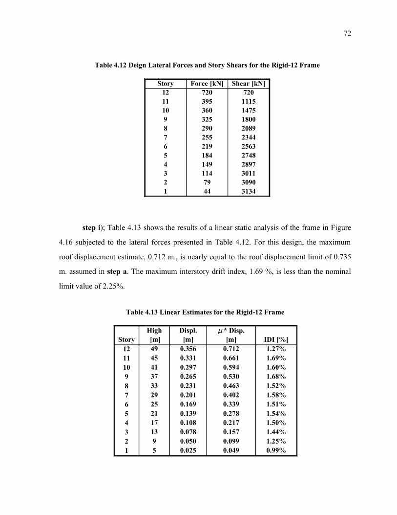
72
step i); Table 4.13 shows the results of a linear static analysis of the frame in Figure
4.16 subjected to the lateral forces presented in Table 4.12. For this design, the maximum
roof displacement estimate, 0.712 m., is nearly equal to the roof displacement limit of 0.735
m. assumed in step a. The maximum interstory drift index, 1.69 %, is less than the nominal
limit value of 2.25%.
Table 4.12 Deign Lateral Forces and Story Shears for the Rigid-12 Frame
Story12 720 72011 395 111510 360 14759 325 18008 290 20897 255 23446 219 25635 184 27484 149 28973 114 30112 79 30901 44 3134
Force [kN] Shear [kN]
Table 4.13 Linear Estimates for the Rigid-12 Frame
Story IDI [%]12 49 0.356 0.712 1.27%11 45 0.331 0.661 1.69%10 41 0.297 0.594 1.60%9 37 0.265 0.530 1.68%8 33 0.231 0.463 1.52%7 29 0.201 0.402 1.58%6 25 0.169 0.339 1.51%5 21 0.139 0.278 1.54%4 17 0.108 0.217 1.50%3 13 0.078 0.157 1.44%2 9 0.050 0.099 1.25%1 5 0.025 0.049 0.99%
High [m]
Displ.[m]
µ * Disp.[m]

73
Figure 4.16 Rigid-12 Frame
T1 = 1.25 Sec.
4.00 m
4.00 m
4.00 m
4.00 m
4.00 m
4.00 m
4.00 m
4.00 m
4.00 m
4.00 m
4.00 m
5.00 m
3 @ 8.00 m
W14X455 W14X455 W14X455 W14X455
W14X370 W14X370 W14X370 W14X370
W14X342 W14X342 W14X342 W14X342
W14X283 W14X283 W14X283 W14X283
W14X211 W14X211 W14X211 W14X211
W14X132 W14X132 W14X132 W14X132
W14X132 W14X132 W14X132 W14X132
W14X211 W14X211 W14X211 W14X211
W14X283 W14X283 W14X283 W14X283
W14X342 W14X342 W14X342 W14X342
W14X370 W14X370 W14X370 W14X370
W14X455 W14X455 W14X455 W14X455
W27X194 W27X194 W27X194
W27X194 W27X194 W27X194
W27X161 W27X161 W27X161
W27X161 W27X161 W27X161
W27X146 W27X146 W27X146
W27X146 W27X146 W27X146
W27X129 W27X129 W27X129
W27X129 W27X129 W27X129
W24X104 W24X104 W24X104
W24X104 W24X104 W24X104
W24X68 W24X68 W24X68
W24X68 W24X68 W24X68
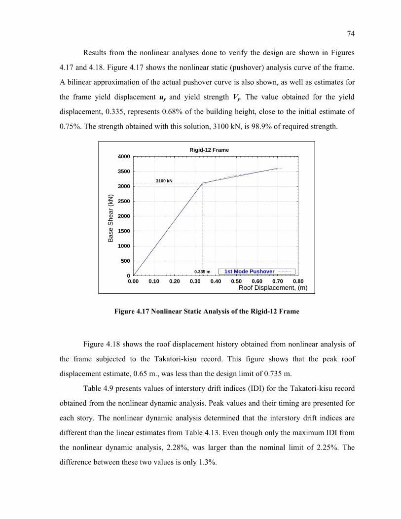
74
Results from the nonlinear analyses done to verify the design are shown in Figures
4.17 and 4.18. Figure 4.17 shows the nonlinear static (pushover) analysis curve of the frame.
A bilinear approximation of the actual pushover curve is also shown, as well as estimates for
the frame yield displacement uy and yield strength Vy. The value obtained for the yield
displacement, 0.335, represents 0.68% of the building height, close to the initial estimate of
0.75%. The strength obtained with this solution, 3100 kN, is 98.9% of required strength.
Figure 4.18 shows the roof displacement history obtained from nonlinear analysis of
the frame subjected to the Takatori-kisu record. This figure shows that the peak roof
displacement estimate, 0.65 m., was less than the design limit of 0.735 m.
Table 4.9 presents values of interstory drift indices (IDI) for the Takatori-kisu record
obtained from the nonlinear dynamic analysis. Peak values and their timing are presented for
each story. The nonlinear dynamic analysis determined that the interstory drift indices are
different than the linear estimates from Table 4.13. Even though only the maximum IDI from
the nonlinear dynamic analysis, 2.28%, was larger than the nominal limit of 2.25%. The
difference between these two values is only 1.3%.
Figure 4.17 Nonlinear Static Analysis of the Rigid-12 Frame
0
500
1000
1500
2000
2500
3000
3500
4000
0.00 0.10 0.20 0.30 0.40 0.50 0.60 0.70 0.80
Rigid-12 Frame
Bas
e S
hear
(kN
)
Roof Displacement, (m)
0.335 m
3100 kN
1st Mode Pushover

75
Table 4.14 Interstory Drift Indices from Nonlinear Dynamic Analysis of the Rigid-12
Story12 0.81% 6.8411 1.33% 5.5110 1.70% 5.559 1.91% 5.578 1.87% 5.647 1.99% 6.346 2.20% 6.355 2.28% 6.364 2.11% 6.363 1.74% 6.342 1.23% 6.291 0.94% 13.57
IDI[%]
Time[Sec]
Figure 4.18 Roof Displacement from Nonlinear Dynamic Analysis of the Rigid-12 Frame
-0.80
-0.60
-0.40
-0.20
0.00
0.20
0.40
0.60
0.80
0 5 10 15 20 25 30 35 40 45 50
Rigid-12 Frame
Roo
f Dis
plac
emen
t (m
)
Time (sec)
Maximum Displacement = 0.650 m.
Design record: Takatori-kisu

76
4.7 Analysis of Results
This section summarizes some results obtained from the 4 frames designed using the
proposed methodology. The discussion is focused in four aspects: roof displacement control,
interstory drift index control, stability of yield displacement estimate, and required minimum
strength and its relation to the fundamental period of vibration.
4.7.1 Roof Displacement Control
Table 4.15 presents results of peak roof displacement. Linear estimates along with
results from nonlinear dynamic analysis are shown. Ratios of peak linear and nonlinear roof
displacement to the roof limit imposed for design, and the ratio of the linear estimate to the
nonlinear result are included. The table also contains the mean and the standard deviation of
this ratios.
The ratios of the nonlinear dynamic peak roof displacement to the roof displacement
limit are all less than one for all the frames, with a mean of 0.902 and a small dispersion.
This indicates that the proposed design methodology was effective in limiting the roof
displacement of the frames. The ratios of the linear estimates to nonlinear dynamic results
were larger than one for all the frames, with a mean of 1.143, indicating that linear static
analyses overestimated the actual response in these frames. Additionally, the ratio of linear
static analysis estimates to the intended roof displacement limit was nearly one for all the
frames, with a mean of 1.030. Based on these data, results from linear static analysis scaled
by the system displacement ductility may possible be an upper bound estimate of peak roof
displacement. Furthermore, linear estimates may be directly compared with the intended roof
limits.
Table 4.15 Peak Roof Displacement Comparison
Roof Limit Nonlinear Dynamic Linear EstimateFrame [m] Ratio Ratio Ratio
Flexible-4 0.255 0.241 0.94 0.261 1.02 1.08Rigid-4 0.255 0.223 0.87 0.272 1.07 1.22Flexible-12 0.735 0.666 0.91 0.781 1.06 1.17Rigid-12 0.735 0.650 0.88 0.712 0.97 1.10Mean 0.902 1.030 1.143Standard Deviation 0.031 0.045 0.065
L/NLDisp. [m] Disp. [m]

77
4.7.2 Interstory Drift Control
Table 4.16 presents results of peak interstory drift indices. Linear IDI estimates along
with IDI results from nonlinear dynamic analysis, ratios of calculated IDI to the IDI limit
imposed for design, and the ratio of the linear to the nonlinear IDI results are included. The
mean and the standard deviation of the ratios are also shown.
The ratio of nonlinear dynamic interstory drift index to interstory drift index limit,
although larger then one for three out of the four frames, the excess was very small (1.01,
1.05). The mean for this ratio was 0.951, indicating that proposed design methodology was
effective in controlling the peak interstory drift index of the frames.
In general, the ratios of the linear estimates to nonlinear dynamic results were smaller
than one, with a mean of 0.862. These results shows that the use of linear analysis to estimate
peak interstory drift index consistently underestimated the actual peak interstory drift index.
4.7.3 Yield Displacement Stability
Table 4.17 shows means and standard deviations of the ratio of the yield displacement
to the building height for the 4 frames. For all the frames, this ratio was always inside the
range of (0.6%-0.9%) suggested in step b) of the proposed methodology . The mean, 0.74%,
is in the middle of this range, with very small dispersion.
Table 4.16 Peak Interstory Drift Index Comparison
IDI Limit Nonlinear Dynamic Linear EstimateFrame [%] IDI [%] Ratio IDI [%] Ratio
Flexible-4 2.25% 2.28% 1.01 1.79% 0.79Rigid-4 2.25% 1.64% 0.73 1.92% 1.17Flexible-12 2.25% 2.37% 1.05 1.77% 0.75Rigid-12 2.25% 2.28% 1.01 1.69% 0.74Mean 0.951 0.862Standard Deviation 0.150 0.208
L/NL
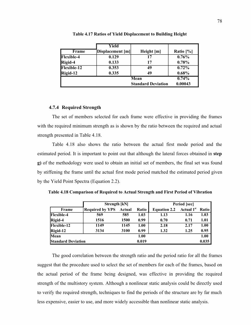
78
4.7.4 Required Strength
The set of members selected for each frame were effective in providing the frames
with the required minimum strength as is shown by the ratio between the required and actual
strength presented in Table 4.18.
Table 4.18 also shows the ratio between the actual first mode period and the
estimated period. It is important to point out that although the lateral forces obtained in step
g) of the methodology were used to obtain an initial set of members, the final set was found
by stiffening the frame until the actual first mode period matched the estimated period given
by the Yield Point Spectra (Equation 2.2).
The good correlation between the strength ratio and the period ratio for all the frames
suggest that the procedure used to select the set of members for each of the frames, based on
the actual period of the frame being designed, was effective in providing the required
strength of the multistory system. Although a nonlinear static analysis could be directly used
to verify the required strength, techniques to find the periods of the structure are by far much
less expensive, easier to use, and more widely accessible than nonlinear static analysis.
Table 4.17 Ratios of Yield Displacement to Building Height
YieldFrame Displacement [m] Height [m] Ratio [%]
Flexible-4 0.129 17 0.76%Rigid-4 0.133 17 0.78%Flexible-12 0.353 49 0.72%Rigid-12 0.335 49 0.68%
Mean 0.74%Standard Deviation 0.00043
Table 4.18 Comparison of Required to Actual Strength and First Period of Vibration
Period [sec]Frame Required by YPS Actual Ratio Equation 2.2 Ratio
Flexible-4 569 585 1.03 1.13 1.16 1.03Rigid-4 1516 1500 0.99 0.70 0.71 1.01Flexible-12 1149 1145 1.00 2.18 2.17 1.00Rigid-12 3134 3100 0.99 1.32 1.25 0.95Mean 1.00 1.00Standard Deviation 0.019 0.035
Strength [kN]Actual 1st

79
4.8 Summary
A methodology for the design of regular multistory buildings is introduced. The
methodology is intended to directly limit the roof displacement to a prescribed value. The
methodology uses Yield Point Spectra, introduced in Chapter 2, to account for nonlinear
behavior in the multistory system. The maximum interstory drift index is limited indirectly
using a coefficient that relates the roof drift index to the maximum interstory drift. Static
linear analysis can be relied on to apply the methodology.
The methodology was illustrated by designing four frames; a set of two 4-story and a
set of two 12-story moment-resistant steel frames. For each set, the design ground motions
were selected such that a flexible and a rigid design were obtained per set of buildings. The
effectiveness of the methodology was validated using nonlinear static and dynamic analysis.
From the results obtained in Chapter 4, the following was observed:
• Yield Point Spectra can be used to design multistory buildings.
• The proposed design methodology is effective for controlling peak roof displacement and
interstory drifts.
• Linear static analysis in conjunction with estimates of system ductilities can be used to
obtain estimates of peak roof displacement.
• Results from linear analysis generally underestimate the peak interstory drift index.
• The ratio of yield displacement to building height seems very stable, and may lie in the
vicinity of the range (0.6%-0.9%) for many moment-resistant steel frames.
80
CHAPTER 5
ANALYSIS OF BUILDING PERFORMANCE USING YIELD POINT SPECTRA
5.1 Introduction
The use of nonlinear static procedures (NSPs) to predict seismic force and
deformation demands for evaluating the performance of new and existing structures is
becoming more common in structural engineering practice. In general, NSPs use nonlinear
static analysis (pushover) and the equivalent SDOF formulation to represent the response of a
multistory building.
This chapter introduces an analysis method, named the YPSA method, in which Yield
Point Spectra are used to estimate peak displacement response, system ductility demands,
and interstory drifts. Just as in existing NSPs, the YPSA method uses nonlinear static
analysis and the equivalent SDOF formulation to predict the seismic behavior of multistory
systems. Therefore, the YPSA method may be classified as a NSP.
In this Chapter, peak displacement response is estimated for the four frames designed
in Chapter 4, two 4-story and two 12-story buildings. The frames are analyzed using four
methodologies: nonlinear dynamic analysis using DRAIN-2DX (Powell et al., 1993), the
Displacement Coefficient Method (FEMA-273/274, 1997), the Capacity Spectrum Method
(ATC-40, 1996), and the YPSA method as described in this chapter. For each method, the
peak displacement response of the frames is estimated under the action of 15 ground motions
(Section 2.7.1). The frames are identified in this Chapter as Flexible-4, Rigid-4, Flexible-12,
and Rigid-12.
Additionally, the YPSA method is used to evaluate three procedures to estimate peak
interstory drift index (IDI). One procedure uses a single deformed shape for estimating IDI
following conventional practice, the other two estimate IDI using the first and second elastic
mode shapes.
In each case, results obtained from nonlinear dynamic analysis were used as a basis
for evaluating the estimates obtained with the simplified procedures. Results are reported and
compared using plots and statistical analysis (means and standard deviations).

81
5.2 Nonlinear Static Procedures
Nonlinear Static Procedures (NSPs) are simplified techniques used to estimate the
maximum expected response of a building during a ground motion. To achieve this objective,
NSPs represent the response of a multistory building using an equivalent SDOF system. Two
key aspects of these procedures are the nonlinear static analysis (pushover), used to
determine the overall capacity of a structure, and the equivalent SDOF modeling technique.
This section reviews the nonlinear static analysis required by NSPs, and briefly
summarizes two existing Nonlinear Static Procedures: the Displacement Coefficient Method
(DCM) and of the Capacity Spectrum Method (CSM). The equivalent SDOF modeling
technique is reviewed in Chapter 3. The NSPs are described in more detail in the FEMA-273
(Guidelines for the Seismic Rehabilitation of Building) and the ATC-40 (Seismic Evaluation
and Retrofit of Concrete Buildings) documents.
Similar to existing NSPs, the YPSA method uses nonlinear static analysis and the
equivalent SDOF formulation to predict the seismic behavior of multistory systems. The
conceptual development for the YPSA method is presented in Section 5.3
5.2.1 Nonlinear Static Analysis
NSPs require the determination of the structural capacity of the building. The
structural capacity is defined as the structure's ability to resist seismic demands, and depends
on the strength and deformation capacities of the individual components of the structure.
To determine capacities beyond the elastic limits, some form of nonlinear analysis,
such as the pushover procedure is required. In a pushover analysis, the mathematical model
of the building, incorporating directly the nonlinear load-deformation characteristic of
individual components, is subjected to monotonically increasing lateral forces or
displacements until a target displacement is reached. The target displacement is intended to
represent the maximum displacement likely to be experienced during the design earthquake.
Pushover analysis permits one to obtain the yield strength and yield displacement
(yield point) of a structure. The yield strength and yield displacement are transformed, using
Equations 5.1 to 5.3, to represent the yield point of an equivalent SDOF system required by
NSP methods.

82
(5.1)
(5.2)
(5.3)
where: uysdof is the yield displacement of SDOF,
uymdof is the yield displacement of MDOF,
Vy is the yield strength of the MDOF,Cy
is the yield strength coefficient,Wt is the total weight of the building,α is the modal mass coefficient,Leq/Meq is the participation factor,{φ} mode shape representing the building lateral deformation,Meq is defined as {φ }T M {φ },Leq is defined as {φ }T M {1}, andMt is defined as {1}T M {1}.
The lateral loads (or displacements) used in the pushover analysis are applied in
profiles that approximate the likely deformed shape of the building responding to the ground
motion induced forces.
In this study, the selected deformed shape ({φ}) used as pattern for the pushover
analysis required in the NSP methods is the same deformed shape used to apply the
equivalent SDOF formulation (Equation 5.1 to 5.3).
5.2.1.1 Selecting the Appropriate Deformed Shape {φ}
In Chapter 3, values for the participation factor and for the modal mass coefficient
were generated using approximate deformed shapes. Those values were used in Chapter 4 to
design the four frames that are analyzed in this chapter.
The approximate deformed shapes shown in Chapter 3 may still be used when
engineers want to check an existing design. Even though, following recommendation
associated with the sophistication Level 3 of the ATC-40 (Seismic Evaluation and Retrofit of
u y
SDOF=
M eq
Leq
u y
MDOF
C y =V
y
α ⋅W t
α =Leq
2
Meq⋅M
t

83
Concrete Buildings), in this study the pattern used as a profile to displace or "push" the
building was proportional to the fundamental mode shape. This same shape, normalized to
one at the top, was used to apply the equivalent SDOF modeling technique.
Beside the ATC-40 recommendation, the reason to assume the fundamental mode as
the deformed shape is the idea that the fundamental mode shape would lead to more accurate
results compared to other approximate deformed shapes. Additionally, mode shapes are
easily obtained using widely available computer programs.
5.2.2 Displacement Coefficient Method
The Displacement Coefficient Method (DCM) uses nonlinear static pushover analysis
of the building and a modified version of the equal displacement rule to estimate maximum
displacements for MDOF buildings. Similar to other NSPs, the DCM also uses parameters
derived from the equivalent SDOF methodology to obtain the displacement estimation.
In the DCM method, peak displacement response is estimated as the product of a
series of coefficients and the spectral displacement of an elastic oscillator.
The peak displacement estimate, δt is given by
(5.4)
where: C0 is a modification factor to relate spectral displacement to expected roofdisplacement,
C1 is a modification factor to relate expected maximum displacements todisplacement calculated for linear elastic response,
C2 is a modification factor to represent the type of hysteretic response,C3 is a modification factor to represent dynamic P-∆ effects,Sa is the response spectrum acceleration,Te is the effective fundamental period of the building andg is the acceleration of gravity.
The coefficient C0 is equivalent to the participation factor. Its value was taken equal
to the ratio Leq/Meq defined in this study. The coefficient C1 accounts for the trend that the
peak displacement of short period nonlinears system exceeds thatof a linear elastic system
having the same period and damping. For short period systems, Te < T0 (T0 = characteristic
period of the ground motion); C1 is given by
δt = C 0C 1C 2 C 3 S a
T e2
4π2 g

84
(5.5)
where R is the ratio of elastic strength demand to calculated yield strength coefficient. For
long period systems, Te > T0 , the "equal displacement rule" applies and C1 = 1.0. The values
of C2 and C3 were taken as 1.0 for all the cases.
Results for the DCM were obtained using a computer program written for this
research. For each case, the response spectrum acceleration, Sa, corresponding to the
effective period of the building, was obtained from the actual acceleration records. No
smoothed spectrum was used here. Values for the characteristic period of the ground motion
T0 are listed in Table 2.2. The computer program implementing the DCM is included as
Appendix B.
5.2.3 Capacity Spectrum Method
The Capacity Spectrum Method is an iterative process in which it is assumed that the
peak displacement response of a nonlinear system can be estimated as the response of an
elastic system having reduced stiffness and increased damping.
In the Capacity Spectrum Method, a first displacement is estimated using the initial
stiffness of the structure assuming elastic response with damping equal to 5% of critical
damping. Then, an estimate of the secant stiffness is obtained using the intersection of the
displacement estimate and the curve representing the capacity spectrum. Effective viscous
damping is revised based on the displacement estimate. Using the current secant stiffness and
adjusted damping, a new displacement estimate is obtained. The iterations continue until
satisfactory convergence is obtained.
A computer program was written to implement the Capacity Spectrum Method. The
program was run using all the parameters corresponding to the Structural Behavior Type A
(New Buildings) as defined in ATC-40. The actual ground motion records were used to
estimate the elastic response of the 5% damped oscillator, and this response was reduced to
account for the increasing damping using equations found in ATC-40. The computer
program is included as Appendix C.
C1=
T e+(RB1 )T 0
T e R

85
5.3 Conceptual Development of the YPSA Method
Similar to others NSPs, the YPSA method requires that the yield strength and yield
displacement of the structure be expressed in terms of the yield strength coefficient (Cy) and
yield displacement of an equivalent single-degree-of-freedom (uysdof). This is done using
Equations 5.1 to 5.3
5.3.1 Estimating Peak Displacement Using the YPSA Method
In the YPSA method, the peak displacement estimate of a MDOF system can be
obtained using equation 5.6 for any assumed deformed shape {φ} as
(5.6)
where: uusdof is the estimated peak displacement of the MDOF system,
Leq/Meq is the participation factor for the assumed deformed shape,æ is the system displacement ductility, andmax(uel
sdof) is the maximum elastic displacement of the equivalent SDOF.
The YPS used for the analysis allow to determine the type of response (linear or
nonlinear) expected for the structure. Depending on the type of response, the maximum
elastic displacement of the equivalent SDOF system, max(uelsdof), or the system displacement
ductility, æ, are estimated form the YPS for use in Equation 5.6.
For nonlinear response (æ > 1), the system displacement ductility is estimated form
the YPS while the maximum elastic displacement of the equivalent SDOF, max(uelsdof), must
be taken equal to the yield displacement of the equivalent SDOF system.
For elastic response (æ ≤ 1), the system displacement ductility must be taken equal to
1 in Equation 5.6 and the maximum elastic displacement of the equivalent SDOF system is
estimated form the YPS.
Examples showing the use of Equation 5.6 for elastic and a nonlinear responses are
presented in Section 5.4.2.
uu
mdof=
Leq
Meq
µ max (uel
sdof)

86
5.3.2 Estimating Interstory Drift Index Using the YPSA Method
Although the value of maximum roof displacement is a direct way to quantify the
overall response of a building, it provides no direct information about localized deformation
within a structure. Typically, seismic codes dictate requirements to control the interstory drift
in each story rather than the peak roof displacement. The interstory drift index (IDI) is
defined as the displacement of any floor relative to the floor immediately below, normalized
by the story height.
Investigators have quantified the interstory drift index in recent years (Qi and
Moehle, 1991; Collins, Wen and Foutch, 1995; Lepage, 1997). In general, the peak IDI can
be expressed as the roof drift index times a coefficient of distortion. The roof drift index is
defined as the peak roof displacement normalized by building height. The coefficient of
distortion is defined as the ratio of the peak interstory drift index to the average drift index.
In general, the coefficient of distortion, and therefore the IDI, is based on the
deformed shape of the building at the moment the peak roof displacement occurs. Since one
hypothesis of the equivalent SDOF methodology is that the deformed shape of the structure
remains constant during the response, values of the peak IDI depends on the deformed shape
assumed in applying the equivalent SDOF methodology. Consistent with this hypothesis, the
interstory drift index profile of the structure may be estimated as
(5.7)
where: IDIj is the estimated interstory drift index for story j,uu
mdof is the peak roof displacement of the structure (Equation 5.6), based on theassumed deformed shape {φ}, and
IDIj(φ) is the modal interstory drift index for story j, defined as the interstory driftindexed calculated for the assumed deformed shape {φ}.
Results from previous work indicate that use of the average drift ratio combined with
the coefficient of distortion to estimate peak IDI is less accurate than the estimates for peak
roof displacement. These previous results suggest that the use of only one deformed shape,
may be inadequate for accurately estimating interstory drift indices.
Combinations of two deformed shapes may be used to obtain improved interstory
drift index estimates. The same procedure used to obtain the peak roof displacement based on
IDIj= uu
mdof⋅IDI
j(φ)
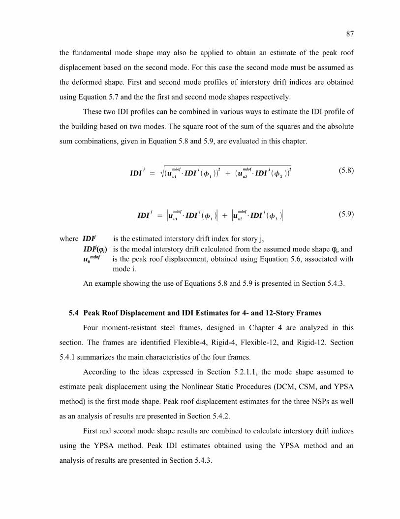
87
the fundamental mode shape may also be applied to obtain an estimate of the peak roof
displacement based on the second mode. For this case the second mode must be assumed as
the deformed shape. First and second mode profiles of interstory drift indices are obtained
using Equation 5.7 and the the first and second mode shapes respectively.
These two IDI profiles can be combined in various ways to estimate the IDI profile of
the building based on two modes. The square root of the sum of the squares and the absolute
sum combinations, given in Equation 5.8 and 5.9, are evaluated in this chapter.
(5.8)
(5.9)
where IDIj is the estimated interstory drift index for story j,IDIj(φi) is the modal interstory drift calculated from the assumed mode shape φi, anduu
mdof is the peak roof displacement, obtained using Equation 5.6, associated withmode i.
An example showing the use of Equations 5.8 and 5.9 is presented in Section 5.4.3.
5.4 Peak Roof Displacement and IDI Estimates for 4- and 12-Story Frames
Four moment-resistant steel frames, designed in Chapter 4 are analyzed in this
section. The frames are identified Flexible-4, Rigid-4, Flexible-12, and Rigid-12. Section
5.4.1 summarizes the main characteristics of the four frames.
According to the ideas expressed in Section 5.2.1.1, the mode shape assumed to
estimate peak displacement using the Nonlinear Static Procedures (DCM, CSM, and YPSA
method) is the first mode shape. Peak roof displacement estimates for the three NSPs as well
as an analysis of results are presented in Section 5.4.2.
First and second mode shape results are combined to calculate interstory drift indices
using the YPSA method. Peak IDI estimates obtained using the YPSA method and an
analysis of results are presented in Section 5.4.3.
IDIj= (u
u1
mdof⋅IDI
j(φ
1))
2+ (u
u2
mdof⋅IDI
j(φ
2))
2
IDIj= |uu1
mdof⋅IDI
j(φ1 )| + |uu2
mdof⋅IDI
j(φ2 )|

88
5.4.1 Characteristics of Frames
Table 5.1 shows values corresponding to the first and second mode shapes and modal
interstory drift indices for the 4-story frames. Table 5.2 has similar information for the 12-
story buildings. All the mode shapes are normalized with respect to the displacement of the
top of the frame.
The data contained in Tables 5.1 and 5.2 are plotted in Figures 5.1 and 5.2
respectively. Figure 5.1(a) plots the first and second mode shapes while Figure 5.1(b) plots
the modal interstory drift indices for the 4-story frames. Figure 5.2 is similar to Figure 5.1
but for the 12-story buildings.
Table 5.1 First and Second Mode Shapes and Modal Interstory Drift Indices of the Flexible-4and Rigid-4 Frames
Story Flexible-4 Rigid-4
Height [m]4 1.0000 3.66% 1.0000 27.74% 1.0000 5.03% 1.0000 31.14%4 0.8536 6.45% -0.1097 23.34% 0.7989 7.08% -0.2457 21.33%4 0.5957 7.06% -1.0432 -3.35% 0.5157 6.04% -1.0989 -5.88%5 0.3134 6.27% -0.9093 -18.19% 0.2743 5.49% -0.8638 -17.28%
1st Mode IDI(φ1) 2nd mode IDI(φ2) 1st Mode IDI(φ1) 2nd mode IDI(φ2)
Table 5.2 First and Second Mode Shapes and Modal Interstory Drift Indices of the Flexible-12 and Rigid-12 Frames
Story Flexible-12 Rigid-12
Height [m]4 1.0000 1.13% 1.0000 7.23% 1.0000 1.40% 1.0000 8.24%4 0.9546 1.70% 0.7109 9.96% 0.9442 2.09% 0.6703 11.23%4 0.8868 1.87% 0.3124 9.04% 0.8605 2.15% 0.2211 9.15%4 0.8120 2.17% -0.0490 8.15% 0.7747 2.35% -0.1448 7.53%4 0.7254 2.24% -0.3751 5.77% 0.6806 2.18% -0.4460 4.39%4 0.6356 2.37% -0.6057 3.45% 0.5932 2.31% -0.6215 2.25%4 0.5409 2.29% -0.7437 0.86% 0.5008 2.23% -0.7113 0.04%4 0.4492 2.34% -0.7780 -1.28% 0.4117 2.28% -0.7129 -1.78%4 0.3556 2.29% -0.7267 -3.08% 0.3205 2.22% -0.6419 -3.20%4 0.2640 2.34% -0.6034 -4.58% 0.2317 2.13% -0.5138 -4.13%4 0.1704 2.19% -0.4203 -5.17% 0.1465 1.84% -0.3487 -4.21%5 0.0828 1.66% -0.2136 -4.27% 0.0728 1.46% -0.1804 -3.61%
1st Mode IDI(φ1) 2nd mode IDI(φ2) 1st Mode IDI(φ1) 2nd mode IDI(φ2)

89
(a)
(b)
Figure 5.1 Mode Shapes and Profiles of Modal IDI for the 4-Story Frames
0.0
0.2
0.4
0.6
0.8
1.0
-1.00 -0.50 0.00 0.50 1.00
Bui
ldin
g H
eigh
t [%
]
Shape Amplitude
1st Mode Flexible-42nd Mode Flexible-41st Mode Rigid-42nd Mode Rigid-4
0
1
2
3
4
0 2 4 6 8
Flexible-4 Rigid-4
Sto
ry
Modal Interstory Drift Indices (%)
First Mode
-35-25-15 -5 5 15 25 35
Flexible-4 Rigid-4
Sto
ry
Modal Interstory Drift Indices (%)
First Mode Second Mode
0 2 4 6 8
Flexible-4 Rigid-4
Sto
ry
Modal Interstory Drift Indices (%)
First Mode Second Mode First Mode
-35-25-15 -5 5 15 25 350
1
2
3
4
Flexible-4 Rigid-4
Sto
ry
Modal Interstory Drift Indices (%)
First Mode Second Mode First Mode Second Mode
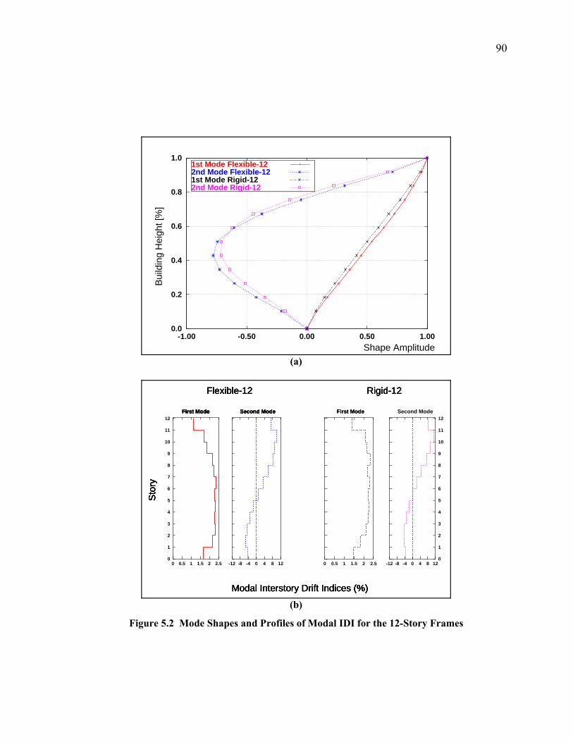
90
(a)
(b)
Figure 5.2 Mode Shapes and Profiles of Modal IDI for the 12-Story Frames
0.0
0.2
0.4
0.6
0.8
1.0
-1.00 -0.50 0.00 0.50 1.00
Bui
ldin
g H
eigh
t [%
]
Shape Amplitude
1st Mode Flexible-122nd Mode Flexible-121st Mode Rigid-122nd Mode Rigid-12
0
1
2
3
4
5
6
7
8
9
10
11
12
0 0.5 1 1.5 2 2.5
Flexible-12 Rigid-12
Sto
ry
Modal Interstory Drift Indices (%)
First Mode
-12 -8 -4 0 4 8 12
Flexible-12 Rigid-12
Sto
ry
Modal Interstory Drift Indices (%)
First Mode Second Mode
0 0.5 1 1.5 2 2.5
Flexible-12 Rigid-12
Sto
ry
Modal Interstory Drift Indices (%)
First Mode Second Mode First Mode
-12 -8 -4 0 4 8 120
1
2
3
4
5
6
7
8
9
10
11
12
Flexible-12 Rigid-12
Sto
ry
Modal Interstory Drift Indices (%)
First Mode Second Mode First Mode Second Mode
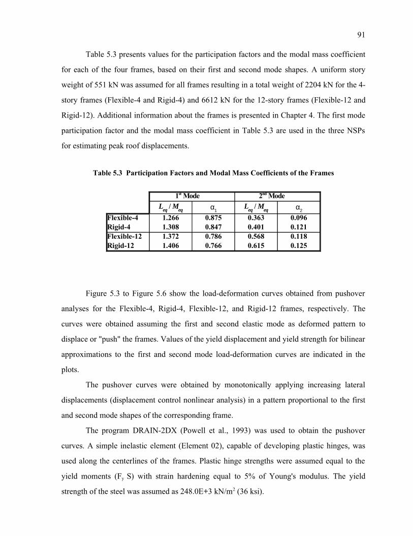
91
Table 5.3 presents values for the participation factors and the modal mass coefficient
for each of the four frames, based on their first and second mode shapes. A uniform story
weight of 551 kN was assumed for all frames resulting in a total weight of 2204 kN for the 4-
story frames (Flexible-4 and Rigid-4) and 6612 kN for the 12-story frames (Flexible-12 and
Rigid-12). Additional information about the frames is presented in Chapter 4. The first mode
participation factor and the modal mass coefficient in Table 5.3 are used in the three NSPs
for estimating peak roof displacements.
Figure 5.3 to Figure 5.6 show the load-deformation curves obtained from pushover
analyses for the Flexible-4, Rigid-4, Flexible-12, and Rigid-12 frames, respectively. The
curves were obtained assuming the first and second elastic mode as deformed pattern to
displace or "push" the frames. Values of the yield displacement and yield strength for bilinear
approximations to the first and second mode load-deformation curves are indicated in the
plots.
The pushover curves were obtained by monotonically applying increasing lateral
displacements (displacement control nonlinear analysis) in a pattern proportional to the first
and second mode shapes of the corresponding frame.
The program DRAIN-2DX (Powell et al., 1993) was used to obtain the pushover
curves. A simple inelastic element (Element 02), capable of developing plastic hinges, was
used along the centerlines of the frames. Plastic hinge strengths were assumed equal to the
yield moments (Fy S) with strain hardening equal to 5% of Young's modulus. The yield
strength of the steel was assumed as 248.0E+3 kN/m2 (36 ksi).
Table 5.3 Participation Factors and Modal Mass Coefficients of the Frames
Flexible-4 1.266 0.875 0.363 0.096Rigid-4 1.308 0.847 0.401 0.121Flexible-12 1.372 0.786 0.568 0.118Rigid-12 1.406 0.766 0.615 0.125
1st Mode 2nd ModeLeq / Meq α1
Leq / Meq α2
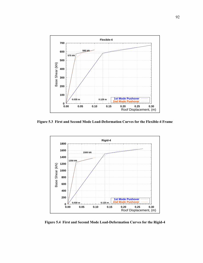
92
Figure 5.3 First and Second Mode Load-Deformation Curves for the Flexible-4 Frame
0
100
200
300
400
500
600
700
0.00 0.05 0.10 0.15 0.20 0.25 0.30
Flexible-4
Bas
e S
hear
(kN
)
Roof Displacement, (m)
0.129 m
585 kN
0.035 m
575 kN
1st Mode Pushover2nd Mode Pushover
Figure 5.4 First and Second Mode Load-Deformation Curves for the Rigid-4
0
200
400
600
800
1000
1200
1400
1600
1800
0.00 0.05 0.10 0.15 0.20 0.25 0.30
Rigid-4
Bas
e S
hear
(kN
)
Roof Displacement, (m)
0.133 m
1500 kN
0.030 m
1250 kN
1st Mode Pushover2nd Mode Pushover

93
Figure 5.5 First and Second Mode Load-Deformation Curves for the Flexible-12
0
200
400
600
800
1000
1200
1400
0.00 0.10 0.20 0.30 0.40 0.50 0.60 0.70 0.80
Flexible-12
Bas
e S
hear
(kN
)
Roof Displacement, (m)
0.353 m
1145 kN
0.11 m
954 kN
1st Mode Pushover2nd Mode Pushover
Figure 5.6 First and Second Mode Load-Deformation Curves for the Rigid-12
0
500
1000
1500
2000
2500
3000
3500
4000
0.00 0.10 0.20 0.30 0.40 0.50 0.60 0.70 0.80
Rigid-12
Bas
e S
hear
(kN
)
Roof Displacement, (m)
0.335 m
3100 kN
0.091 m
2150 kN
1st Mode Pushover2nd Mode Pushover
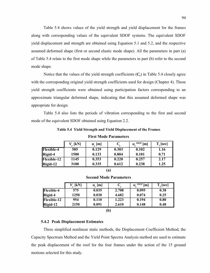
94
Table 5.4 shows values of the yield strength and yield displacement for the frames
along with corresponding values of the equivalent SDOF systems. The equivalent SDOF
yield displacement and strength are obtained using Equation 5.1 and 5.2, and the respective
assumed deformed shape (first or second elastic mode shape). All the parameters in part (a)
of Table 5.4 relate to the first mode shape while the parameters in part (b) refer to the second
mode shape.
Notice that the values of the yield strength coefficients (Cy) in Table 5.4 closely agree
with the corresponding original yield strength coefficients used for design (Chapter 4). Those
yield strength coefficients were obtained using participation factors corresponding to an
approximate triangular deformed shape, indicating that this assumed deformed shape was
appropriate for design.
Table 5.4 also lists the periods of vibration corresponding to the first and second
mode of the equivalent SDOF obtained using Equation 2.2.
5.4.2 Peak Displacement Estimates
Three simplified nonlinear static methods, the Displacement Coefficient Method, the
Capacity Spectrum Method and the Yield Point Spectra Analysis method are used to estimate
the peak displacement of the roof for the four frames under the action of the 15 ground
motions selected for this study.
Table 5.4 Yield Strength and Yield Displacement of the Frames
First Mode Parameters
(a)
Second Mode Parameters
(b)
Flexible-4 585 0.129 0.303 0.102 1.16Rigid-4 1500 0.133 0.804 0.101 0.71Flexible-12 1145 0.353 0.220 0.257 2.17Rigid-12 3100 0.335 0.612 0.238 1.25
Vy [kN] uy [m] Cy uy SDOF
[m] T1 [sec]
Flexible-4 575 0.035 2.708 0.095 0.38Rigid-4 1250 0.030 4.682 0.074 0.25Flexible-12 954 0.110 1.223 0.194 0.80Rigid-12 2150 0.091 2.610 0.148 0.48
Vy [kN] uy [m] Cy uy SDOF
[m] T2 [sec]

95
The results of each simplified procedure are compared with peak displacement
obtained from nonlinear dynamic displacement histories analyses of the frames. Results for
each procedure are compared using plots and using simple statistical analysis.
A numerical example is provided to illustrate how the YPSA method is used to
estimate the peak displacement response of a multistory frame. The Yield Point Spectra
corresponding to the 1940 N-S component of the El Centro record (IV40ELCN.180) and
Equation 5.6 are used to estimate peak displacements for the Flexible-4 and Rigid-4 frames.
The participation factor for the Flexible-4 frame is 1.266 and for the Rigid-4 frame is
1.308. These factors are in Table 5.3. The equivalent SDOF yield displacements for the
Flexible-4 and Rigid-4 frames are 10.2 and 10.1 cm. and the yield strength coefficients are
0.303 and 0.804 respectively (see Table 5.4a).
The equivalent SDOF yield points for these two frames are plotted in Figure 5.7; with
'x' used for the Flexible-4 frame and '+' used for the Rigid-4 frame. The periods of vibration
of the equivalents SDOF systems are represented by dotted diagonal lines.
Figure 5.7 Yield Points for the 4-Story Frames
'x' indicates Yield Point for Flexible-4
'+' indicates Yield Point for Rigid-4
1Ε−03
1Ε−02
1Ε−01
1Ε+00
1Ε−04 1Ε−03 1Ε−02 1Ε−01 1Ε+00
Bilinear for IV40ELCN.180, 5% Damping, 10% Post Yield Stiffness
Yie
ld S
tren
gth
Coe
ffici
ent (
C )y
Yield Displacement, (m)
x
+
T= 0.05
T= 0.1
T= 1.0 T= 10.0
µ=1µ=2µ=4µ=8
1Ε−03
1Ε−02
1Ε−01
1Ε+00
1Ε−04 1Ε−03 1Ε−02 1Ε−01 1Ε+00
Bilinear for IV40ELCN.180, 5% Damping, 10% Post Yield Stiffness
Yie
ld S
tren
gth
Coe
ffici
ent (
C )y
Yield Displacement, (m)
x
+
T= 0.05
T= 0.1
T= 1.0 T= 10.01Ε−03
1Ε−02
1Ε−01
1Ε+00
1Ε−04 1Ε−03 1Ε−02 1Ε−01 1Ε+00
Bilinear for IV40ELCN.180, 5% Damping, 10% Post Yield Stiffness
Yie
ld S
tren
gth
Coe
ffici
ent (
C )y
Yield Displacement, (m)
x
+
T= 0.05
T= 0.1
T= 1.0 T= 10.01Ε−03
1Ε−02
1Ε−01
1Ε+00
1Ε−04 1Ε−03 1Ε−02 1Ε−01 1Ε+00
Bilinear for IV40ELCN.180, 5% Damping, 10% Post Yield Stiffness
Yie
ld S
tren
gth
Coe
ffici
ent (
C )y
Yield Displacement, (m)
x
+
T= 0.05
T= 0.1
T= 1.0 T= 10.01Ε−03
1Ε−02
1Ε−01
1Ε+00
1Ε−04 1Ε−03 1Ε−02 1Ε−01 1Ε+00
Bilinear for IV40ELCN.180, 5% Damping, 10% Post Yield Stiffness
Yie
ld S
tren
gth
Coe
ffici
ent (
C )y
Yield Displacement, (m)
x
+
T= 0.05
T= 0.1
T= 1.0 T= 10.01Ε−03
1Ε−02
1Ε−01
1Ε+00
1Ε−04 1Ε−03 1Ε−02 1Ε−01 1Ε+00
Bilinear for IV40ELCN.180, 5% Damping, 10% Post Yield Stiffness
Yie
ld S
tren
gth
Coe
ffici
ent (
C )y
Yield Displacement, (m)
x
+
T= 0.05
T= 0.1
T= 1.0 T= 10.01Ε−03
1Ε−02
1Ε−01
1Ε+00
1Ε−04 1Ε−03 1Ε−02 1Ε−01 1Ε+00
Bilinear for IV40ELCN.180, 5% Damping, 10% Post Yield Stiffness
Yie
ld S
tren
gth
Coe
ffici
ent (
C )y
Yield Displacement, (m)
x
+
T= 0.05
T= 0.1
T= 1.0 T= 10.01Ε−03
1Ε−02
1Ε−01
1Ε+00
1Ε−04 1Ε−03 1Ε−02 1Ε−01 1Ε+00
Bilinear for IV40ELCN.180, 5% Damping, 10% Post Yield Stiffness
Yie
ld S
tren
gth
Coe
ffici
ent (
C )y
Yield Displacement, (m)
x
+
T= 0.05
T= 0.1
T= 1.0 T= 10.01Ε−03
1Ε−02
1Ε−01
1Ε+00
1Ε−04 1Ε−03 1Ε−02 1Ε−01 1Ε+00
Bilinear for IV40ELCN.180, 5% Damping, 10% Post Yield Stiffness
Yie
ld S
tren
gth
Coe
ffici
ent (
C )y
Yield Displacement, (m)
x
+
T= 0.05
T= 0.1
T= 1.0 T= 10.01Ε−03
1Ε−02
1Ε−01
1Ε+00
1Ε−04 1Ε−03 1Ε−02 1Ε−01 1Ε+00
Bilinear for IV40ELCN.180, 5% Damping, 10% Post Yield Stiffness
Yie
ld S
tren
gth
Coe
ffici
ent (
C )y
Yield Displacement, (m)
x
+
T= 0.05
T= 0.1
T= 1.0 T= 10.01Ε−03
1Ε−02
1Ε−01
1Ε+00
1Ε−04 1Ε−03 1Ε−02 1Ε−01 1Ε+00
Bilinear for IV40ELCN.180, 5% Damping, 10% Post Yield Stiffness
Yie
ld S
tren
gth
Coe
ffici
ent (
C )y
Yield Displacement, (m)
x
+
T= 0.05
T= 0.1
T= 1.0 T= 10.01Ε−03
1Ε−02
1Ε−01
1Ε+00
1Ε−04 1Ε−03 1Ε−02 1Ε−01 1Ε+00
Bilinear for IV40ELCN.180, 5% Damping, 10% Post Yield Stiffness
Yie
ld S
tren
gth
Coe
ffici
ent (
C )y
Yield Displacement, (m)
x
+
T= 0.05
T= 0.1
T= 1.0 T= 10.01Ε−03
1Ε−02
1Ε−01
1Ε+00
1Ε−04 1Ε−03 1Ε−02 1Ε−01 1Ε+00
Bilinear for IV40ELCN.180, 5% Damping, 10% Post Yield Stiffness
Yie
ld S
tren
gth
Coe
ffici
ent (
C )y
Yield Displacement, (m)
x
+
T= 0.05
T= 0.1
T= 1.0 T= 10.01Ε−03
1Ε−02
1Ε−01
1Ε+00
1Ε−04 1Ε−03 1Ε−02 1Ε−01 1Ε+00
Bilinear for IV40ELCN.180, 5% Damping, 10% Post Yield Stiffness
Yie
ld S
tren
gth
Coe
ffici
ent (
C )y
Yield Displacement, (m)
x
+
T= 0.05
T= 0.1
T= 1.0 T= 10.01Ε−03
1Ε−02
1Ε−01
1Ε+00
1Ε−04 1Ε−03 1Ε−02 1Ε−01 1Ε+00
Bilinear for IV40ELCN.180, 5% Damping, 10% Post Yield Stiffness
Yie
ld S
tren
gth
Coe
ffici
ent (
C )y
Yield Displacement, (m)
x
+
T= 0.05
T= 0.1
T= 1.0 T= 10.01Ε−03
1Ε−02
1Ε−01
1Ε+00
1Ε−04 1Ε−03 1Ε−02 1Ε−01 1Ε+00
Bilinear for IV40ELCN.180, 5% Damping, 10% Post Yield Stiffness
Yie
ld S
tren
gth
Coe
ffici
ent (
C )y
Yield Displacement, (m)
x
+
T= 0.05
T= 0.1
T= 1.0 T= 10.01Ε−03
1Ε−02
1Ε−01
1Ε+00
1Ε−04 1Ε−03 1Ε−02 1Ε−01 1Ε+00
Bilinear for IV40ELCN.180, 5% Damping, 10% Post Yield Stiffness
Yie
ld S
tren
gth
Coe
ffici
ent (
C )y
Yield Displacement, (m)
x
+
T= 0.05
T= 0.1
T= 1.0 T= 10.01Ε−03
1Ε−02
1Ε−01
1Ε+00
1Ε−04 1Ε−03 1Ε−02 1Ε−01 1Ε+00
Bilinear for IV40ELCN.180, 5% Damping, 10% Post Yield Stiffness
Yie
ld S
tren
gth
Coe
ffici
ent (
C )y
Yield Displacement, (m)
x
+
T= 0.05
T= 0.1
T= 1.0 T= 10.01Ε−03
1Ε−02
1Ε−01
1Ε+00
1Ε−04 1Ε−03 1Ε−02 1Ε−01 1Ε+00
Bilinear for IV40ELCN.180, 5% Damping, 10% Post Yield Stiffness
Yie
ld S
tren
gth
Coe
ffici
ent (
C )y
Yield Displacement, (m)
x
+
T= 0.05
T= 0.1
T= 1.0 T= 10.01Ε−03
1Ε−02
1Ε−01
1Ε+00
1Ε−04 1Ε−03 1Ε−02 1Ε−01 1Ε+00
Bilinear for IV40ELCN.180, 5% Damping, 10% Post Yield Stiffness
Yie
ld S
tren
gth
Coe
ffici
ent (
C )y
Yield Displacement, (m)
x
+
T= 0.05
T= 0.1
T= 1.0 T= 10.01Ε−03
1Ε−02
1Ε−01
1Ε+00
1Ε−04 1Ε−03 1Ε−02 1Ε−01 1Ε+00
Bilinear for IV40ELCN.180, 5% Damping, 10% Post Yield Stiffness
Yie
ld S
tren
gth
Coe
ffici
ent (
C )y
Yield Displacement, (m)
x
+
T= 0.05
T= 0.1
T= 1.0 T= 10.01Ε−03
1Ε−02
1Ε−01
1Ε+00
1Ε−04 1Ε−03 1Ε−02 1Ε−01 1Ε+00
Bilinear for IV40ELCN.180, 5% Damping, 10% Post Yield Stiffness
Yie
ld S
tren
gth
Coe
ffici
ent (
C )y
Yield Displacement, (m)
x
+
T= 0.05
T= 0.1
T= 1.0 T= 10.01Ε−03
1Ε−02
1Ε−01
1Ε+00
1Ε−04 1Ε−03 1Ε−02 1Ε−01 1Ε+00
Bilinear for IV40ELCN.180, 5% Damping, 10% Post Yield Stiffness
Yie
ld S
tren
gth
Coe
ffici
ent (
C )y
Yield Displacement, (m)
x
+
T= 0.05
T= 0.1
T= 1.0 T= 10.0

96
In Figure 5.7 it can be seen that the yield point corresponding to the Flexible-4 frame
lies between the curves corresponding to ductility of 1 and 2. This yield point is located at
about 16% of the distance measured from the curve corresponding to a ductility of 1 to the
curve corresponding to a ductility of 2. Therefore, the ductility demand associated with this
frame responding to El Centro record is estimated as 20.16 = 1.117, and its peak displacement
is estimated, using Equation 5.6, as:
uumdof = (1. 266) (1.117) (10.2) = 14.4 cm. (5.10)
Figure 5.7 also shows that the yield point corresponding to the Rigid-4 frame lies
beyond the curve corresponding to ductility of 1; therefore, the response of this frame
responding to El Centro record is elastic and the ductility demand to be used in Equation 5.6
must be taken equal to one.
An arrow indicates that the equivalent SDOF system associated with this frame has a
maximum elastic displacement of approximately 7.70 cm. Therefore, using Equation 5.6, the
estimate of the peak displacement for Rigid-4 frame under El Centro record is equal to:
uumdof = (1. 308) (1.0) (7.7) = 10.1 cm. (5.11)
5.4.2.1 Numerical Results
The following figures and tables present results for maximum peak displacement
estimated using the YPSA Method, the Displacement Coefficient Method, and the Capacity
Spectrum Method. Peak displacements determined by nonlinear dynamic analyses are
reported along with displacement estimates obtained using the NSPs.
The participation factors (Leq/Meq) are in Table 5.3, and the equivalent SDOF
parameters for the frames are in Table 5.4a.
Peak displacements estimated by the YPSA method are obtained using Equation 5.6
and Yield Point Spectra for the 15 ground motion records considered. For all the frames, the
system displacement ductility (æ) or maximum elastic displacement of the equivalent SDOF
(max(uelsdof)) are read from the YPS in the same way as it was illustrated using Figure 5.7.
These YPS are presented in Appendix D, Figures D.1(a) to D.30(a), at the end of this report.
Tables 5.5 to 5.8 summarize the data used with Equation 5.6.

97
Results for the Displacement Coefficient Method and the Capacity Spectrum Method
were obtained using computer programs specially written for this research. These computer
programs are included in Appendix B and C at the end of this work. Tables 5.9 to 5.12
summarize the results for these NSPs.
For all the nonlinear static methods, a post-yield stiffness of 10% of the initial
stiffness and damping equal to 5% of critical damping was assumed. For the nonlinear
dynamic analysis performed with DRAIN 2DX, the damping parameters for the four frames
were set to produce 5% critical damping in the first mode of vibration. The damping
parameters were set to also produce 5% critical damping in the 4th and 6th modes for the 4-
and 12-story frames, respectively.
Figures 5.8 to 5.11 contain two plots that help to visualize and compare the results
obtained with the three simplified NSPs.
In the upper plots of these figures (part a), the peak roof displacement obtained using
DRAIN-2DX is plotted on the abscissa while the peak roof displacement estimate obtained
with the NSPs are plotted on the ordinate. The diagonal line represents perfect correlation
between the peak displacements obtained with the dynamic nonlinear analysis of the frames
and the simplified method estimates. Any points below this line represent a displacement
underestimation on the part of the simplified method, while points above this line represent
displacement overestimation. A dotted vertical line indicates the yield displacement for the
frames. This line allows to gauge the accuracy of the NSPs as a function of the degree of
nonlinearity in the system.
The lower plot (part b), of Figures 5.8 to 5.11 show the different ground motion
records on the abscissa while the ordinate plots the ratio of the NSPs peak displacement
estimates and nonlinear dynamic analysis results. The earthquakes are arranged on the
abscissa following the order used in Table 5.5. Data supporting theses figures is presented in
Tables 5.5 to 5.12.
Part (a) and (b) of Figures 5.8 to 5.11 complement each other; part (a) displays the
magnitude of the peak displacement response and the accuracy achieved for each of the
NSPs, and part (b) shows the accuracy of the NSPs with respect to each ground motion
record.

98
(a)
(b)
Figure 5.8 Peak Roof Displacement Comparisons for the Flexible-4 Frame
0
20
40
60
80
100
0 20 40 60 80 100
Flexible-4
Dis
plac
emen
t Est
imat
es [c
m]
DRAIN-2DX Displacement [cm]
YPSA DCM CSM
0
20
40
60
80
100
0 20 40 60 80 100
Flexible-4
Dis
plac
emen
t Est
imat
es [c
m]
DRAIN-2DX Displacement [cm]
0
0.5
1
1.5
2Flexible-4
Rat
io E
stim
atio
n/D
RA
IN-2
DX
Dis
plac
emen
t
Short Long Forward
Wn Bb Sp Cr Ce LL Vp EC Jh Mx Lu Sr Nh Sy Ko
YPSA DCM CSM

99
(a)
(b)
Figure 5.9 Peak Roof Displacement Comparisons for the Rigid-4 Frame
0
5
10
15
20
25
30
35
40
0 5 10 15 20 25 30 35 40
Rigid-4
Dis
plac
emen
t Est
imat
es [c
m]
DRAIN-2DX Displacement [cm]
YPSA DCM CSM
0
5
10
15
20
25
30
35
40
0 5 10 15 20 25 30 35 40
Rigid-4
Dis
plac
emen
t Est
imat
es [c
m]
DRAIN-2DX Displacement [cm]
0
0.5
1
1.5
2Rigid-4
Rat
io E
stim
atio
n/D
RA
IN-2
DX
Dis
plac
emen
t
Short Long Forward
Wn Bb Sp Cr Ce LL Vp EC Jh Mx Lu Sr Nh Sy Ko
YPSA DCM CSM

100
(a)
(b)
Figure 5.10 Peak Roof Displacement Comparison for the Flexible-12 Frame
0
20
40
60
80
100
120
140
0 20 40 60 80 100 120 140
Flexible-12
Dis
plac
emen
t Est
imat
es [c
m]
DRAIN-2DX Displacement [cm]
YPSA DCM CSM
0
20
40
60
80
100
120
140
0 20 40 60 80 100 120 140
Flexible-12
Dis
plac
emen
t Est
imat
es [c
m]
DRAIN-2DX Displacement [cm]
0
0.5
1
1.5
2Flexible-12
Rat
io E
stim
atio
n/D
RA
IN-2
DX
Dis
plac
emen
t
Short Long Forward
Wn Bb Sp Cr Ce LL Vp EC Jh Mx Lu Sr Nh Sy Ko
YPSA DCM CSM

101
(a)
(b)
Figure 5.11 Peak Roof Displacement Comparison for the Rigid-12 Frame
0
20
40
60
80
100
120
0 20 40 60 80 100 120
Rigid-12
Dis
plac
emen
t Est
imat
es [c
m]
DRAIN-2DX Displacement [cm]
YPSA DCM CSM
0
20
40
60
80
100
120
0 20 40 60 80 100 120
Rigid-12
Dis
plac
emen
t Est
imat
es [c
m]
DRAIN-2DX Displacement [cm]
0
0.5
1
1.5
2Rigid-12
Rat
io E
stim
atio
n/D
RA
IN-2
DX
Dis
plac
emen
t
Short Long Forward
Wn Bb Sp Cr Ce LL Vp EC Jh Mx Lu Sr Nh Sy Ko
YPSA DCM CSM
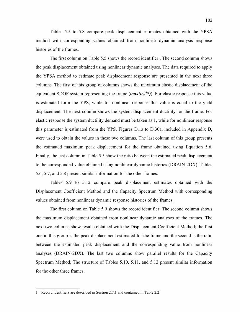
102
Tables 5.5 to 5.8 compare peak displacement estimates obtained with the YPSA
method with corresponding values obtained from nonlinear dynamic analysis response
histories of the frames.
The first column on Table 5.5 shows the record identifier1. The second column shows
the peak displacement obtained using nonlinear dynamic analyses. The data required to apply
the YPSA method to estimate peak displacement response are presented in the next three
columns. The first of this group of columns shows the maximum elastic displacement of the
equivalent SDOF system representing the frame (max(uelsdof)). For elastic response this value
is estimated form the YPS, while for nonlinear response this value is equal to the yield
displacement. The next column shows the system displacement ductility for the frame. For
elastic response the system ductility demand must be taken as 1, while for nonlinear response
this parameter is estimated from the YPS. Figures D.1a to D.30a, included in Appendix D,
were used to obtain the values in these two columns. The last column of this group presents
the estimated maximum peak displacement for the frame obtained using Equation 5.6.
Finally, the last column in Table 5.5 show the ratio between the estimated peak displacement
to the corresponded value obtained using nonlinear dynamic histories (DRAIN-2DX). Tables
5.6, 5.7, and 5.8 present similar information for the other frames.
Tables 5.9 to 5.12 compare peak displacement estimates obtained with the
Displacement Coefficient Method and the Capacity Spectrum Method with corresponding
values obtained from nonlinear dynamic response histories of the frames.
The first column on Table 5.9 shows the record identifier. The second column shows
the maximum displacement obtained from nonlinear dynamic analyses of the frames. The
next two columns show results obtained with the Displacement Coefficient Method; the first
one in this group is the peak displacement estimated for the frame and the second is the ratio
between the estimated peak displacement and the corresponding value from nonlinear
analyses (DRAIN-2DX). The last two columns show parallel results for the Capacity
Spectrum Method. The structure of Tables 5.10, 5.11, and 5.12 present similar information
for the other three frames.
1 Record identifiers are described in Section 2.7.1 and contained in Table 2.2
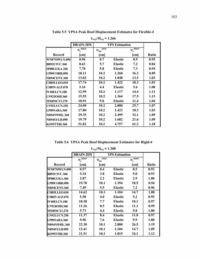
103
Table 5.6 YPSA Peak Roof Displacement Estimates for Rigid-4
LEQ/MEQ = 1.308
Record æ Ratio0.57 0.4 Elastic 0.5 0.925.34 3.8 Elastic 5.0 0.932.87 2.2 Elastic 2.9 1.00
19.70 10.1 1.394 18.5 0.947.49 5.5 Elastic 7.2 0.96
14.62 10.1 1.104 14.7 1.005.50 4.0 Elastic 5.2 0.95
10.38 7.7 Elastic 10.1 0.9711.26 8.5 Elastic 11.1 0.995.73 4.4 Elastic 5.8 1.00
11.37 8.4 Elastic 11.0 0.979.96 7.6 Elastic 9.9 1.00
22.30 10.1 2.000 26.5 1.1913.41 10.1 1.104 14.7 1.0921.51 10.1 1.819 24.1 1.12
DRAIN-2DX YPS Estimationuu
MDOF
[cm]uelas
SDOF
[cm]uu
MDOF
[cm]WN87MWLN.090BB92CIVC.360SP88GUKA.360LP89CORR.090NR94CENT.360CH85LLEO.010CH85VALP.070IV40ELCN.180LN92JOSH.360MX85SCT1.270LN92LUCN.250LP89SARA.360NR94NWHL.360NR94SYLH.090KO95TTRI.360
Table 5.5 YPSA Peak Roof Displacement Estimates for Flexible-4
LEQ/MEQ = 1.266
Record æ Ratio0.96 0.7 Elastic 0.9 0.958.63 5.7 Elastic 7.2 0.847.78 5.8 Elastic 7.3 0.9418.11 10.2 1.260 16.2 0.8913.02 10.2 1.048 13.5 1.0317.74 10.2 1.422 18.3 1.035.16 4.4 Elastic 5.6 1.0812.99 10.2 1.117 14.4 1.1115.55 10.2 1.364 17.5 1.1310.91 9.0 Elastic 11.4 1.0424.09 10.2 2.000 25.7 1.0717.80 10.2 1.423 18.3 1.0329.35 10.2 2.499 32.1 1.0919.79 10.2 1.682 21.6 1.0951.82 10.2 4.757 61.2 1.18
DRAIN-2DX YPS Estimationuu
MDOF
[cm]uelas
SDOF
[cm]uu
MDOF
[cm]WN87MWLN.090BB92CIVC.360SP88GUKA.360LP89CORR.090NR94CENT.360CH85LLEO.010CH85VALP.070IV40ELCN.180LN92JOSH.360MX85SCT1.270LN92LUCN.250LP89SARA.360NR94NWHL.360NR94SYLH.090KO95TTRI.360

104
Table 5.7 YPSA Peak Roof Displacement Estimates for Flexible-12
LEQ/MEQ = 1.372
Record æ Ratio0.98 0.7 Elastic 1.0 0.99
11.51 5.6 Elastic 7.7 0.677.14 4.3 Elastic 5.9 0.83
23.62 11.0 Elastic 15.1 0.6417.86 12.5 Elastic 17.1 0.9634.22 20.5 Elastic 28.1 0.8210.94 7.3 Elastic 10.0 0.9233.64 22.5 Elastic 30.9 0.9222.77 13.0 Elastic 17.8 0.7869.02 25.7 2.000 70.6 1.0250.69 25.7 1.456 51.4 1.0138.14 25.7 1.129 39.8 1.0451.80 25.7 1.542 54.4 1.0560.82 25.7 1.631 57.6 0.9584.09 25.7 2.456 86.7 1.03
DRAIN-2DX YPS Estimationuu
MDOF
[cm]uelas
SDOF
[cm]uu
MDOF
[cm]WN87MWLN.090BB92CIVC.360SP88GUKA.360LP89CORR.090NR94CENT.360CH85LLEO.010CH85VALP.070IV40ELCN.180LN92JOSH.360MX85SCT1.270LN92LUCN.250LP89SARA.360NR94NWHL.360NR94SYLH.090KO95TTRI.360
Table 5.8 YPSA Peak Roof Displacement Estimates for Rigid-12
LEQ/MEQ = 1.406
Record æ Ratio0.98 0.7 Elastic 0.9 0.9310.04 5.8 Elastic 8.2 0.818.52 6.0 Elastic 8.4 0.9923.39 16.5 Elastic 23.2 0.9916.35 10.7 Elastic 15.0 0.9225.47 18.0 Elastic 25.3 0.999.07 6.0 Elastic 8.4 0.9317.50 11.1 Elastic 15.6 0.8928.37 19.0 Elastic 26.7 0.9414.34 11.0 Elastic 15.5 1.0829.27 20.5 Elastic 28.8 0.9826.45 18.0 Elastic 25.3 0.9655.45 23.8 1.436 48.1 0.8728.47 20.0 Elastic 28.1 0.9965.01 23.8 2.225 74.5 1.15
DRAIN-2DX YPS Estimationuu
MDOF
[cm]uelas
SDOF
[cm]uu
MDOF
[cm]WN87MWLN.090BB92CIVC.360SP88GUKA.360LP89CORR.090NR94CENT.360CH85LLEO.010CH85VALP.070IV40ELCN.180LN92JOSH.360MX85SCT1.270LN92LUCN.250LP89SARA.360NR94NWHL.360NR94SYLH.090KO95TTRI.360
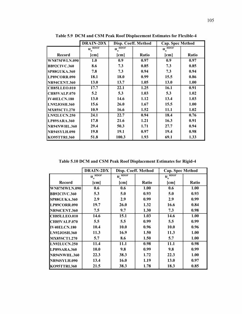
105
Table 5.9 DCM and CSM Peak Roof Displacement Estimates for Flexible-4
Cap. Spec Method
Record Ratio Ratio1.0 0.9 0.97 0.9 0.978.6 7.3 0.85 7.3 0.857.8 7.3 0.94 7.3 0.9418.1 18.0 0.99 15.5 0.8613.0 13.7 1.05 13.0 1.0017.7 22.1 1.25 16.1 0.915.2 5.3 1.03 5.3 1.0213.0 14.6 1.12 13.4 1.0315.6 26.0 1.67 15.5 1.0010.9 16.6 1.52 11.1 1.0224.1 22.7 0.94 18.4 0.7617.8 21.6 1.21 16.3 0.9129.4 50.3 1.71 27.7 0.9419.8 19.1 0.97 19.4 0.9851.8 100.3 1.93 69.1 1.33
DRAIN-2DX Disp. Coeff. Methoduu
MDOF
[cm]uu
MDOF
[cm]uu
MDOF
[cm]WN87MWLN.090BB92CIVC.360SP88GUKA.360LP89CORR.090NR94CENT.360CH85LLEO.010CH85VALP.070IV40ELCN.180LN92JOSH.360MX85SCT1.270LN92LUCN.250LP89SARA.360NR94NWHL.360NR94SYLH.090KO95TTRI.360
Table 5.10 DCM and CSM Peak Roof Displacement Estimates for Rigid-4
Cap. Spec Method
Record Ratio Ratio0.6 0.6 1.00 0.6 1.005.3 5.0 0.93 5.0 0.932.9 2.9 0.99 2.9 0.99
19.7 26.0 1.32 16.6 0.847.5 9.7 1.30 7.3 0.98
14.6 15.1 1.03 14.6 1.005.5 5.5 0.99 5.5 0.99
10.4 10.0 0.96 10.0 0.9611.3 16.9 1.50 11.3 1.005.7 8.6 1.50 5.7 1.00
11.4 11.1 0.98 11.1 0.9810.0 9.8 0.99 9.8 0.9922.3 38.3 1.72 22.3 1.0013.4 16.0 1.19 13.0 0.9721.5 38.3 1.78 18.3 0.85
DRAIN-2DX Disp. Coeff. Methoduu
MDOF
[cm]uu
MDOF
[cm]uu
MDOF
[cm]WN87MWLN.090BB92CIVC.360SP88GUKA.360LP89CORR.090NR94CENT.360CH85LLEO.010CH85VALP.070IV40ELCN.180LN92JOSH.360MX85SCT1.270LN92LUCN.250LP89SARA.360NR94NWHL.360NR94SYLH.090KO95TTRI.360

106
Table 5.11 DCM and CSM Peak Roof Displacement Estimates for Flexible-12
Cap. Spec Method
Record Ratio Ratio1.0 1.0 1.00 0.9 0.9611.5 7.7 0.67 7.6 0.667.1 5.9 0.83 5.8 0.8223.6 13.8 0.58 15.1 0.6417.9 17.3 0.97 16.2 0.9134.2 27.4 0.80 31.3 0.9210.9 9.1 0.84 10.8 0.9933.6 29.6 0.88 27.3 0.8122.8 17.0 0.75 17.7 0.7869.0 128.5 1.86 70.5 1.0250.7 47.1 0.93 39.1 0.7738.1 40.6 1.06 36.4 0.9651.8 57.0 1.10 41.0 0.7960.8 72.8 1.20 51.2 0.8484.1 148.5 1.77 79.4 0.94
DRAIN-2DX Disp. Coeff. Methoduu
MDOF
[cm]uu
MDOF
[cm]uu
MDOF
[cm]WN87MWLN.090BB92CIVC.360SP88GUKA.360LP89CORR.090NR94CENT.360CH85LLEO.010CH85VALP.070IV40ELCN.180LN92JOSH.360MX85SCT1.270LN92LUCN.250LP89SARA.360NR94NWHL.360NR94SYLH.090KO95TTRI.360
Table 5.12 DCM and CSM Peak Roof Displacement Estimates for Rigid-12
Cap. Spec Method
Record Ratio Ratio1.0 0.9 0.94 0.9 0.9410.0 7.7 0.77 7.7 0.778.5 8.7 1.02 8.7 1.0223.4 23.1 0.99 23.1 0.9916.4 14.6 0.89 14.6 0.8925.5 24.6 0.97 24.6 0.979.1 8.8 0.97 8.8 0.9717.5 15.5 0.89 15.5 0.8928.4 27.3 0.96 26.5 0.9314.3 21.7 1.51 15.0 1.0429.3 29.2 1.00 29.2 1.0026.5 25.1 0.95 25.1 0.9555.5 59.7 1.08 42.3 0.7628.5 29.0 1.02 28.9 1.0265.0 127.6 1.96 53.6 0.82
DRAIN-2DX Disp. Coeff. Methoduu
MDOF
[cm]uu
MDOF
[cm]uu
MDOF
[cm]WN87MWLN.090BB92CIVC.360SP88GUKA.360LP89CORR.090NR94CENT.360CH85LLEO.010CH85VALP.070IV40ELCN.180LN92JOSH.360MX85SCT1.270LN92LUCN.250LP89SARA.360NR94NWHL.360NR94SYLH.090KO95TTRI.360
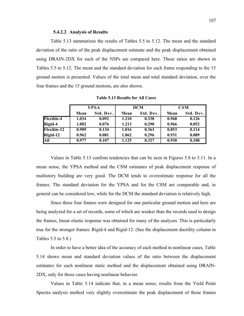
107
5.4.2.2 Analysis of Results
Table 5.13 summarizes the results of Tables 5.5 to 5.12. The mean and the standard
deviation of the ratio of the peak displacement estimate and the peak displacement obtained
using DRAIN-2DX for each of the NSPs are compared here. These ratios are shown in
Tables 5.5 to 5.12. The mean and the standard deviation for each frame responding to the 15
ground motion is presented. Values of the total mean and total standard deviation, over the
four frames and the 15 ground motions, are also shown.
Values in Table 5.13 confirm tendencies that can be seen in Figures 5.8 to 5.11. In a
mean sense, the YPSA method and the CSM estimates of peak displacement response of
multistory building are very good. The DCM tends to overestimate response for all the
frames. The standard deviation for the YPSA and for the CSM are comparable and, in
general can be considered low, while for the DCM the standard deviation is relatively high.
Since these four frames were designed for one particular ground motion and here are
being analyzed for a set of records, some of which are weaker than the records used to design
the frames, linear elastic response was obtained for many of the analyses. This is particularly
true for the stronger frames: Rigid-4 and Rigid-12. (See the displacement ductility column in
Tables 5.5 to 5.8.)
In order to have a better idea of the accuracy of each method in nonlinear cases, Table
5.14 shows mean and standard deviation values of the ratio between the displacement
estimates for each nonlinear static method and the displacement obtained using DRAIN-
2DX, only for those cases having nonlinear behavior.
Values in Table 5.14 indicate that, in a mean sense, results from the Yield Point
Spectra analysis method very slightly overestimate the peak displacement of those frames
Table 5.13 Results for All Cases
DCMMean Mean Mean
Flexible-4 1.034 0.092 1.210 0.338 0.968 0.126Rigid-4 1.002 0.076 1.213 0.290 0.966 0.052Flexible-12 0.909 0.134 1.016 0.363 0.853 0.114Rigid-12 0.962 0.081 1.062 0.296 0.931 0.089All 0.977 0.107 1.125 0.327 0.930 0.108
YPSA CSMStd. Dev. Std. Dev. Std. Dev.

108
having nonlinear response, with a small standard deviation for three out of the four frames.
For Rigid-12 the standard deviation was quite high compared with the other frames.
For the Capacity Spectrum Method, mean values show that this method tends to
underestimate response in the nonlinear cases considered. The standard deviation for the
nonlinear cases are similar to corresponding values shown in Table 5.13.
The Displacement Coefficient Method tends to overestimate response even more for
the nonlinear cases. The standard deviation for this method becomes larger for the nonlinear
cases considered.
5.4.3 Estimates of Interstory Drift Indices
Interstory drift is traditionally calculated based on the deformed shape of the building
under the action of equivalent static design forces. As an alternative, interstory drift can be
estimated using the first mode shape, normalized to one on the top, amplified by the the roof
peak displacement. This alternate approach is used in Equation 5.7. In both cases interstory
drift is estimated using a single deformed shape.
Table 4.16 in Chapter 4 shows that use of only one deformed shape underestimates
interstory drift indices for the four frames considered. The YPSA method provides an easy
way to obtain interstory drift index estimates based on combinations of two mode shapes.
In this section, interstory drift index estimates calculated using the YPSA method
and one mode shape (equation 5.7) and combinations of the first two mode shapes (Equations
5.8 and 5.9) are compared with corresponding peak interstory drift indices obtained from
nonlinear dynamic analysis of the frames (DRAIN-2DX).
Yield Point Spectra with damping set to 2.8% of the critical damping were used for
the estimations related with the second mode shape to reflect the lower damping assigned to
Table 5.14 Results for NonLinear Cases
DCMMean Mean Mean
Flexible-4 1.066 0.077 1.285 0.357 0.973 0.150Rigid-4 1.069 0.099 1.409 0.327 0.932 0.079Flexible-12 1.018 0.038 1.320 0.394 0.887 0.101Rigid-12 1.007 0.197 1.519 0.626 0.793 0.044
YPSA CSMStd. Dev. Std. Dev. Std. Dev.

109
this mode in the nonlinear dynamic analysis performed using DRAIN-2DX. The mean value
of the second mode damping for the four frames analyzed in DRAIN-2DX was
approximately 2.8% of the critical damping.
Following is a numerical example to illustrate the use of Yield Point Spectra to
estimate interstory drift indices. The interstory drift index for the 4th story of the Flexible-4
frame responding to the 1940 N-S component of the El Centro record (IV40ELCN.180) is
estimated using Equation 5.7 (one mode) and Equations 5.8 and 5.9 (combinations of two
modes).
Figures 5.1b and 5.2b show profiles of the the first and second modal interstory drift
indices for each of the four frames. The data plotted in these figures are contained in Tables
5.1 and 5.2. The modal interstory drift index for the 4th story of the Flexible-4 frame is 3.66%
and 27.7% for the first and second modes respectively (See Figure 5.1b or Table 5.1).
In Section 5.4.2, the Yield Point Spectra corresponding to the the 1940 N-S
component of the El Centro record (IV40ELCN.180) and first mode parameters were used to
estimate a peak displacement response of 14.4E-2 m. for the Flexible-4 frame. A similar
calculation, using second mode parameters is done to estimate the peak displacement
response of the same frame in the second mode.
For the Flexible-4 frame, the second mode participation factor is 0.363 and can be
obtained from Table 5.3. The equivalent SDOF yield displacement and the yield strength
coefficient in the second mode are 9.5E-2 m. and 2.708 respectively (see Table 5.4b).
Figure 5.12 shows the Yield Point Spectra corresponding to the El Centro record
(IV40ELCN.180) for a damping equal to 2.8% of critical damping. The equivalent SDOF
second mode yield point for the Flexible-4 frame is indicated using a 'x' sign, in Figure 5.12.
The equivalent second mode period of vibration is shown by a dotted diagonal line.
In Figure 5.12 it can be seen that the yield point lies beyond the curve corresponding
to ductility of 1; therefore, the equivalent SDOF associated with second mode of vibration
for this building has a maximum elastic displacement of approximately 2.5E-2 m. and a
displacement ductility equal to 1.

110
Using Equation 5.6, the peak displacement estimate for the second mode of the
Flexible-4 frame under El Centro record is equal to,
(uumdof)2 = (0. 363) (1.0) (2.5E-2) = 9.08E-3 m. (5.12)
Interstory drift indices for the 4th story of Flexible-4 frame can now be obtained using
Equations 5.7 to 5.9.
Using Equation 5.7,
IDI4 = (14.4E-2) (3.66%) = 0.527% (5.13)
Equation 5.8 leads to
IDI4 = √ ((14.4E-2 ⋅ 3.66%)2 + (9.08E-3 ⋅ 27.7%)2 ) = 0.779% (5.14)
Figure 5.12 Second Mode Yield Point for the Flexible-4 Frame
'x' indicates Second Mode Yield Point for Flexible-4
1Ε−03
1Ε−02
1Ε−01
1Ε+00
1Ε−04 1Ε−03 1Ε−02 1Ε−01 1Ε+00
Bilinear for IV40ELCN.180, 2.8% Damping, 10% Post Yield Stiffness
Yie
ld S
tren
gth
Coe
ffici
ent (
C )y
Yield Displacement, (m)
x
T= 0.05
T= 0.1
T= 1.0 T= 10.0
µ=1µ=2
1Ε−03
1Ε−02
1Ε−01
1Ε+00
1Ε−04 1Ε−03 1Ε−02 1Ε−01 1Ε+00
Bilinear for IV40ELCN.180, 2.8% Damping, 10% Post Yield Stiffness
Yie
ld S
tren
gth
Coe
ffici
ent (
C )y
Yield Displacement, (m)
x
T= 0.05
T= 0.1
T= 1.0 T= 10.01Ε−03
1Ε−02
1Ε−01
1Ε+00
1Ε−04 1Ε−03 1Ε−02 1Ε−01 1Ε+00
Bilinear for IV40ELCN.180, 2.8% Damping, 10% Post Yield Stiffness
Yie
ld S
tren
gth
Coe
ffici
ent (
C )y
Yield Displacement, (m)
x
T= 0.05
T= 0.1
T= 1.0 T= 10.01Ε−03
1Ε−02
1Ε−01
1Ε+00
1Ε−04 1Ε−03 1Ε−02 1Ε−01 1Ε+00
Bilinear for IV40ELCN.180, 2.8% Damping, 10% Post Yield Stiffness
Yie
ld S
tren
gth
Coe
ffici
ent (
C )y
Yield Displacement, (m)
x
T= 0.05
T= 0.1
T= 1.0 T= 10.01Ε−03
1Ε−02
1Ε−01
1Ε+00
1Ε−04 1Ε−03 1Ε−02 1Ε−01 1Ε+00
Bilinear for IV40ELCN.180, 2.8% Damping, 10% Post Yield Stiffness
Yie
ld S
tren
gth
Coe
ffici
ent (
C )y
Yield Displacement, (m)
x
T= 0.05
T= 0.1
T= 1.0 T= 10.01Ε−03
1Ε−02
1Ε−01
1Ε+00
1Ε−04 1Ε−03 1Ε−02 1Ε−01 1Ε+00
Bilinear for IV40ELCN.180, 2.8% Damping, 10% Post Yield Stiffness
Yie
ld S
tren
gth
Coe
ffici
ent (
C )y
Yield Displacement, (m)
x
T= 0.05
T= 0.1
T= 1.0 T= 10.01Ε−03
1Ε−02
1Ε−01
1Ε+00
1Ε−04 1Ε−03 1Ε−02 1Ε−01 1Ε+00
Bilinear for IV40ELCN.180, 2.8% Damping, 10% Post Yield Stiffness
Yie
ld S
tren
gth
Coe
ffici
ent (
C )y
Yield Displacement, (m)
x
T= 0.05
T= 0.1
T= 1.0 T= 10.01Ε−03
1Ε−02
1Ε−01
1Ε+00
1Ε−04 1Ε−03 1Ε−02 1Ε−01 1Ε+00
Bilinear for IV40ELCN.180, 2.8% Damping, 10% Post Yield Stiffness
Yie
ld S
tren
gth
Coe
ffici
ent (
C )y
Yield Displacement, (m)
x
T= 0.05
T= 0.1
T= 1.0 T= 10.01Ε−03
1Ε−02
1Ε−01
1Ε+00
1Ε−04 1Ε−03 1Ε−02 1Ε−01 1Ε+00
Bilinear for IV40ELCN.180, 2.8% Damping, 10% Post Yield Stiffness
Yie
ld S
tren
gth
Coe
ffici
ent (
C )y
Yield Displacement, (m)
x
T= 0.05
T= 0.1
T= 1.0 T= 10.01Ε−03
1Ε−02
1Ε−01
1Ε+00
1Ε−04 1Ε−03 1Ε−02 1Ε−01 1Ε+00
Bilinear for IV40ELCN.180, 2.8% Damping, 10% Post Yield Stiffness
Yie
ld S
tren
gth
Coe
ffici
ent (
C )y
Yield Displacement, (m)
x
T= 0.05
T= 0.1
T= 1.0 T= 10.01Ε−03
1Ε−02
1Ε−01
1Ε+00
1Ε−04 1Ε−03 1Ε−02 1Ε−01 1Ε+00
Bilinear for IV40ELCN.180, 2.8% Damping, 10% Post Yield Stiffness
Yie
ld S
tren
gth
Coe
ffici
ent (
C )y
Yield Displacement, (m)
x
T= 0.05
T= 0.1
T= 1.0 T= 10.01Ε−03
1Ε−02
1Ε−01
1Ε+00
1Ε−04 1Ε−03 1Ε−02 1Ε−01 1Ε+00
Bilinear for IV40ELCN.180, 2.8% Damping, 10% Post Yield Stiffness
Yie
ld S
tren
gth
Coe
ffici
ent (
C )y
Yield Displacement, (m)
x
T= 0.05
T= 0.1
T= 1.0 T= 10.01Ε−03
1Ε−02
1Ε−01
1Ε+00
1Ε−04 1Ε−03 1Ε−02 1Ε−01 1Ε+00
Bilinear for IV40ELCN.180, 2.8% Damping, 10% Post Yield Stiffness
Yie
ld S
tren
gth
Coe
ffici
ent (
C )y
Yield Displacement, (m)
x
T= 0.05
T= 0.1
T= 1.0 T= 10.01Ε−03
1Ε−02
1Ε−01
1Ε+00
1Ε−04 1Ε−03 1Ε−02 1Ε−01 1Ε+00
Bilinear for IV40ELCN.180, 2.8% Damping, 10% Post Yield Stiffness
Yie
ld S
tren
gth
Coe
ffici
ent (
C )y
Yield Displacement, (m)
x
T= 0.05
T= 0.1
T= 1.0 T= 10.01Ε−03
1Ε−02
1Ε−01
1Ε+00
1Ε−04 1Ε−03 1Ε−02 1Ε−01 1Ε+00
Bilinear for IV40ELCN.180, 2.8% Damping, 10% Post Yield Stiffness
Yie
ld S
tren
gth
Coe
ffici
ent (
C )y
Yield Displacement, (m)
x
T= 0.05
T= 0.1
T= 1.0 T= 10.01Ε−03
1Ε−02
1Ε−01
1Ε+00
1Ε−04 1Ε−03 1Ε−02 1Ε−01 1Ε+00
Bilinear for IV40ELCN.180, 2.8% Damping, 10% Post Yield Stiffness
Yie
ld S
tren
gth
Coe
ffici
ent (
C )y
Yield Displacement, (m)
x
T= 0.05
T= 0.1
T= 1.0 T= 10.01Ε−03
1Ε−02
1Ε−01
1Ε+00
1Ε−04 1Ε−03 1Ε−02 1Ε−01 1Ε+00
Bilinear for IV40ELCN.180, 2.8% Damping, 10% Post Yield Stiffness
Yie
ld S
tren
gth
Coe
ffici
ent (
C )y
Yield Displacement, (m)
x
T= 0.05
T= 0.1
T= 1.0 T= 10.01Ε−03
1Ε−02
1Ε−01
1Ε+00
1Ε−04 1Ε−03 1Ε−02 1Ε−01 1Ε+00
Bilinear for IV40ELCN.180, 2.8% Damping, 10% Post Yield Stiffness
Yie
ld S
tren
gth
Coe
ffici
ent (
C )y
Yield Displacement, (m)
x
T= 0.05
T= 0.1
T= 1.0 T= 10.01Ε−03
1Ε−02
1Ε−01
1Ε+00
1Ε−04 1Ε−03 1Ε−02 1Ε−01 1Ε+00
Bilinear for IV40ELCN.180, 2.8% Damping, 10% Post Yield Stiffness
Yie
ld S
tren
gth
Coe
ffici
ent (
C )y
Yield Displacement, (m)
x
T= 0.05
T= 0.1
T= 1.0 T= 10.01Ε−03
1Ε−02
1Ε−01
1Ε+00
1Ε−04 1Ε−03 1Ε−02 1Ε−01 1Ε+00
Bilinear for IV40ELCN.180, 2.8% Damping, 10% Post Yield Stiffness
Yie
ld S
tren
gth
Coe
ffici
ent (
C )y
Yield Displacement, (m)
x
T= 0.05
T= 0.1
T= 1.0 T= 10.01Ε−03
1Ε−02
1Ε−01
1Ε+00
1Ε−04 1Ε−03 1Ε−02 1Ε−01 1Ε+00
Bilinear for IV40ELCN.180, 2.8% Damping, 10% Post Yield Stiffness
Yie
ld S
tren
gth
Coe
ffici
ent (
C )y
Yield Displacement, (m)
x
T= 0.05
T= 0.1
T= 1.0 T= 10.01Ε−03
1Ε−02
1Ε−01
1Ε+00
1Ε−04 1Ε−03 1Ε−02 1Ε−01 1Ε+00
Bilinear for IV40ELCN.180, 2.8% Damping, 10% Post Yield Stiffness
Yie
ld S
tren
gth
Coe
ffici
ent (
C )y
Yield Displacement, (m)
x
T= 0.05
T= 0.1
T= 1.0 T= 10.0

111
and Equation 5.9 to
IDI4 = |(14.4E-2) (3.66%)| + |(9.08E-3) (27.7%)| = 0.779% (5.15)
These three IDI estimations are plotted in Figure 5.14(a) for the IV40ELCN.180
record.
5.4.3.1 Numerical Results
Figures 5.13 to 5.24 help to visualize and compare, on a story-by-story basis, the
interstory drift indices estimated using Equations 5.7 to 5.9. Similar to the peak roof
displacement comparison, results from the nonlinear dynamic analyses are used to evaluate
the accuracy of the results obtained with each of the proposed IDI Equations.
Part (a) of Figures 5.13 to 5.24 compares profiles of estimated peak interstory drift
indices obtained using Equation 5.7 (a single deformed shape) as well as Equations 5.8 and
5.9 (two deformed shapes combinations). The IDI obtained from nonlinear dynamic analyses
are also presented along with results obtained using these three equations.
Part (b) of Figures 5.13 to 5.24 plots, for each story, the ratio of the peak interstory
drift index estimates to the peak IDI computed in the nonlinear dynamic analyses.
The nonlinear interstory drift indices used in Figures 5.13 to 5.24 are the peak
interstory drift indices in each story regardless of the time they occur. In general, in the
dynamic analysis history, peak interstory drifts do not occur simultaneously in all the stories.
Results from the nonlinear dynamic analyses are labeled as 'DRAIN-2DX' in part (a)
of Figures 5.13 to 5.24. Results from Equations 5.7 to 5.9 are labeled as IDI Estimate 1, IDI
Estimate 2, and IDI Estimate 3, respectively in Figures 5.13 to 5.24.
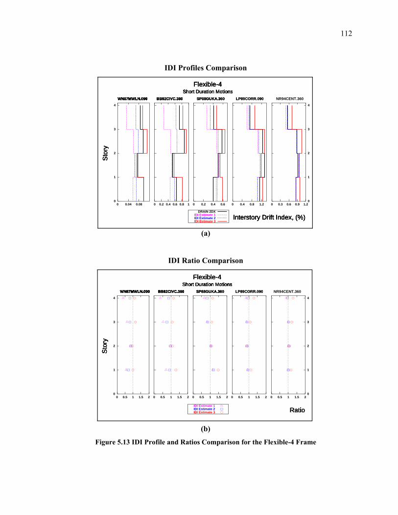
112
IDI Profiles Comparison
(a)
IDI Ratio Comparison
(b)
Figure 5.13 IDI Profile and Ratios Comparison for the Flexible-4 Frame
0
1
2
3
4
0 0.04 0.08
Flexible-4Short Duration Motions
Sto
ry
Interstory Drift Index, (%)
WN87MWLN.090
DRAIN 2DXIDI Estimate 1IDI Estimate 2IDI Estimate 3
0 0.2 0.4 0.6 0.8 1
Flexible-4Short Duration Motions
Sto
ry
Interstory Drift Index, (%)
WN87MWLN.090 BB92CIVC.360
0 0.2 0.4 0.6
Flexible-4Short Duration Motions
Sto
ry
Interstory Drift Index, (%)
WN87MWLN.090 BB92CIVC.360 SP88GUKA.360
0 0.4 0.8 1.2
Flexible-4Short Duration Motions
Sto
ry
Interstory Drift Index, (%)
WN87MWLN.090 BB92CIVC.360 SP88GUKA.360 LP89CORR.090
0 0.3 0.6 0.9 1.20
1
2
3
4
Flexible-4Short Duration Motions
Sto
ry
Interstory Drift Index, (%)
WN87MWLN.090 BB92CIVC.360 SP88GUKA.360 LP89CORR.090 NR94CENT.360
0
1
2
3
4
0 0.5 1 1.5 2
Flexible-4Short Duration Motions
Sto
ry
Ratio
WN87MWLN.090
IDI Estimate 1IDI Estimate 2IDI Estimate 3
0 0.5 1 1.5 2
Flexible-4Short Duration Motions
Sto
ry
Ratio
WN87MWLN.090 BB92CIVC.360
0 0.5 1 1.5 2
Flexible-4Short Duration Motions
Sto
ry
Ratio
WN87MWLN.090 BB92CIVC.360 SP88GUKA.360
0 0.5 1 1.5 2
Flexible-4Short Duration Motions
Sto
ry
Ratio
WN87MWLN.090 BB92CIVC.360 SP88GUKA.360 LP89CORR.090
0 0.5 1 1.5 20
1
2
3
4
Flexible-4Short Duration Motions
Sto
ry
Ratio
WN87MWLN.090 BB92CIVC.360 SP88GUKA.360 LP89CORR.090 NR94CENT.360

113
IDI Profiles Comparison
(a)
IDI Ratio Comparison
(b)
Figure 5.14 IDI Profile and Ratios Comparison for the Flexible-4 Frame
0
1
2
3
4
0 0.4 0.8 1.2 1.6
Flexible-4Long Duration Motions
Sto
ry
Interstory Drift Index, (%)
CH85LLEO.010
DRAIN 2DXIDI Estimate 1IDI Estimate 2IDI Estimate 3
0 0.1 0.2 0.3 0.4 0.5
Flexible-4Long Duration Motions
Sto
ry
Interstory Drift Index, (%)
CH85LLEO.010 CH85VALP.070
0 0.3 0.6 0.9 1.2
Flexible-4Long Duration Motions
Sto
ry
Interstory Drift Index, (%)
CH85LLEO.010 CH85VALP.070 IV40ELCN.180
0 0.3 0.6 0.9 1.2 1.5
Flexible-4Long Duration Motions
Sto
ry
Interstory Drift Index, (%)
CH85LLEO.010 CH85VALP.070 IV40ELCN.180 LN92JOSH.360
0 0.3 0.6 0.90
1
2
3
4
Flexible-4Long Duration Motions
Sto
ry
Interstory Drift Index, (%)
CH85LLEO.010 CH85VALP.070 IV40ELCN.180 LN92JOSH.360 MX85SCT1.270
0
1
2
3
4
0 0.5 1 1.5 2
Flexible-4Long Duration Motions
Sto
ry
Ratio
CH85LLEO.010
IDI Estimate 1IDI Estimate 2IDI Estimate 3
0 0.5 1 1.5 2
Flexible-4Long Duration Motions
Sto
ry
Ratio
CH85LLEO.010 CH85VALP.070
0 0.5 1 1.5 2
Flexible-4Long Duration Motions
Sto
ry
Ratio
CH85LLEO.010 CH85VALP.070 IV40ELCN.180
0 0.5 1 1.5 2
Flexible-4Long Duration Motions
Sto
ry
Ratio
CH85LLEO.010 CH85VALP.070 IV40ELCN.180 LN92JOSH.360
0 0.5 1 1.5 20
1
2
3
4
Flexible-4Long Duration Motions
Sto
ry
Ratio
CH85LLEO.010 CH85VALP.070 IV40ELCN.180 LN92JOSH.360 MX85SCT1.270
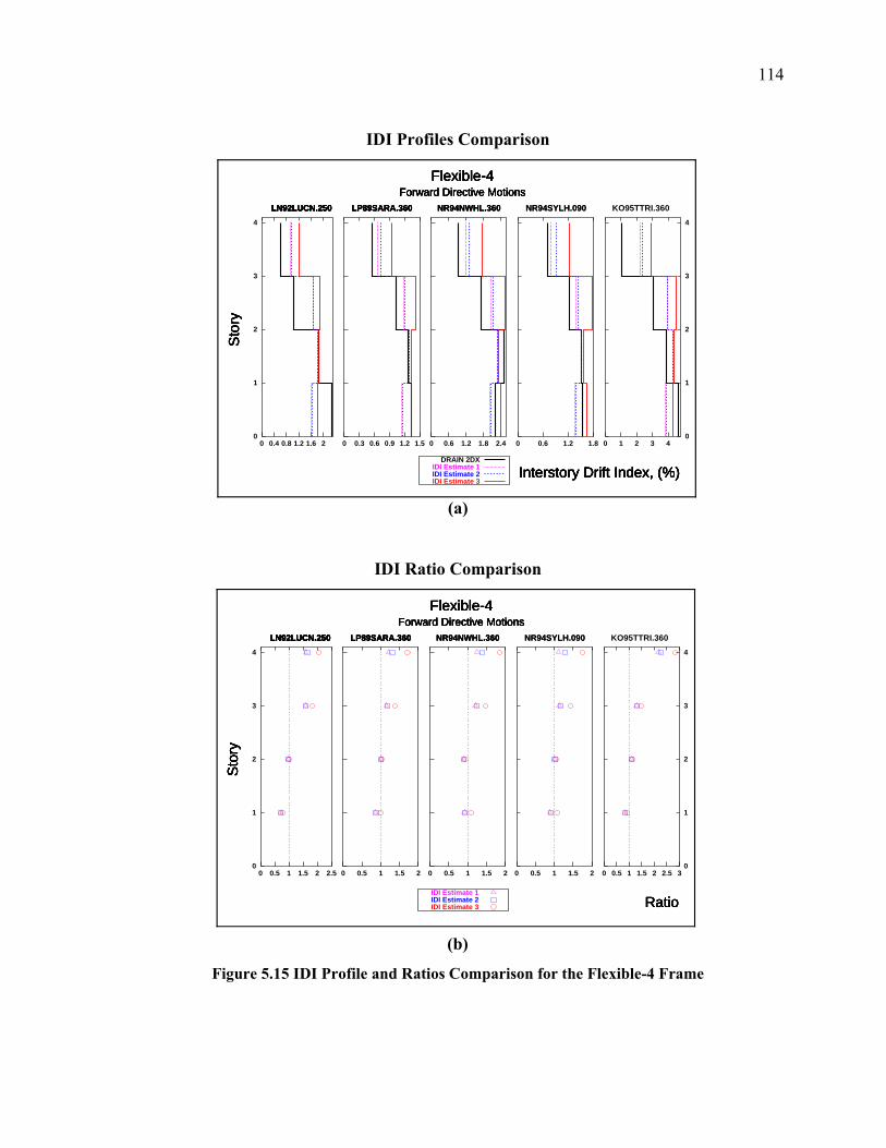
114
IDI Profiles Comparison
(a)
IDI Ratio Comparison
(b)
Figure 5.15 IDI Profile and Ratios Comparison for the Flexible-4 Frame
0
1
2
3
4
0 0.4 0.8 1.2 1.6 2
Flexible-4Forward Directive Motions
Sto
ry
Interstory Drift Index, (%)
LN92LUCN.250
DRAIN 2DXIDI Estimate 1IDI Estimate 2IDI Estimate 3
0 0.3 0.6 0.9 1.2 1.5
Flexible-4Forward Directive Motions
Sto
ry
Interstory Drift Index, (%)
LN92LUCN.250 LP89SARA.360
0 0.6 1.2 1.8 2.4
Flexible-4Forward Directive Motions
Sto
ry
Interstory Drift Index, (%)
LN92LUCN.250 LP89SARA.360 NR94NWHL.360
0 0.6 1.2 1.8
Flexible-4Forward Directive Motions
Sto
ry
Interstory Drift Index, (%)
LN92LUCN.250 LP89SARA.360 NR94NWHL.360 NR94SYLH.090
0 1 2 3 40
1
2
3
4
Flexible-4Forward Directive Motions
Sto
ry
Interstory Drift Index, (%)
LN92LUCN.250 LP89SARA.360 NR94NWHL.360 NR94SYLH.090 KO95TTRI.360
0
1
2
3
4
0 0.5 1 1.5 2 2.5
Flexible-4Forward Directive Motions
Sto
ry
Ratio
LN92LUCN.250
IDI Estimate 1IDI Estimate 2IDI Estimate 3
0 0.5 1 1.5 2
Flexible-4Forward Directive Motions
Sto
ry
Ratio
LN92LUCN.250 LP89SARA.360
0 0.5 1 1.5 2
Flexible-4Forward Directive Motions
Sto
ry
Ratio
LN92LUCN.250 LP89SARA.360 NR94NWHL.360
0 0.5 1 1.5 2
Flexible-4Forward Directive Motions
Sto
ry
Ratio
LN92LUCN.250 LP89SARA.360 NR94NWHL.360 NR94SYLH.090
0 0.5 1 1.5 2 2.5 30
1
2
3
4
Flexible-4Forward Directive Motions
Sto
ry
Ratio
LN92LUCN.250 LP89SARA.360 NR94NWHL.360 NR94SYLH.090 KO95TTRI.360

115
IDI Profiles Comparison
(a)
IDI Ratio Comparison
(b)
Figure 5.16 IDI Profile and Ratios Comparison for the Rigid-4 Frame
0
1
2
3
4
0 0.02 0.04 0.06 0.08
Rigid-4Short Duration Motions
Sto
ry
Interstory Drift Index, (%)
WN87MWLN.090
DRAIN 2DXIDI Estimate 1IDI Estimate 2IDI Estimate 3
0 0.2 0.4 0.6
Rigid-4Short Duration Motions
Sto
ry
Interstory Drift Index, (%)
WN87MWLN.090 BB92CIVC.360
0 0.1 0.2 0.3
Rigid-4Short Duration Motions
Sto
ry
Interstory Drift Index, (%)
WN87MWLN.090 BB92CIVC.360 SP88GUKA.360
0 0.3 0.6 0.9 1.2 1.5
Rigid-4Short Duration Motions
Sto
ry
Interstory Drift Index, (%)
WN87MWLN.090 BB92CIVC.360 SP88GUKA.360 LP89CORR.090
0 0.2 0.4 0.60
1
2
3
4
Rigid-4Short Duration Motions
Sto
ry
Interstory Drift Index, (%)
WN87MWLN.090 BB92CIVC.360 SP88GUKA.360 LP89CORR.090 NR94CENT.360
0
1
2
3
4
0 0.5 1 1.5 2
Rigid-4Short Duration Motions
Sto
ry
Ratio
WN87MWLN.090
IDI Estimate 1IDI Estimate 2IDI Estimate 3
0 0.5 1 1.5 2
Rigid-4Short Duration Motions
Sto
ry
Ratio
WN87MWLN.090 BB92CIVC.360
0 0.5 1 1.5 2
Rigid-4Short Duration Motions
Sto
ry
Ratio
WN87MWLN.090 BB92CIVC.360 SP88GUKA.360
0 0.5 1 1.5 2
Rigid-4Short Duration Motions
Sto
ry
Ratio
WN87MWLN.090 BB92CIVC.360 SP88GUKA.360 LP89CORR.090
0 0.5 1 1.5 20
1
2
3
4
Rigid-4Short Duration Motions
Sto
ry
Ratio
WN87MWLN.090 BB92CIVC.360 SP88GUKA.360 LP89CORR.090 NR94CENT.360
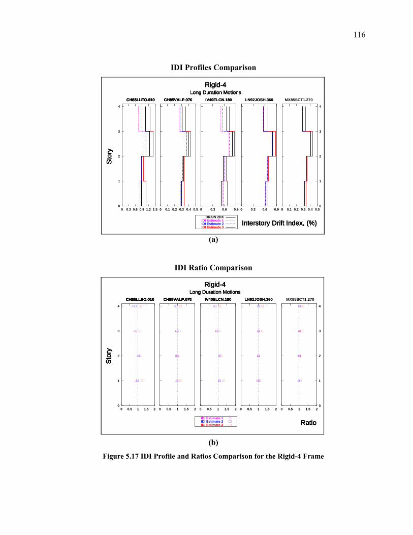
116
IDI Profiles Comparison
(a)
IDI Ratio Comparison
(b)
Figure 5.17 IDI Profile and Ratios Comparison for the Rigid-4 Frame
0
1
2
3
4
0 0.3 0.6 0.9 1.2 1.5
Rigid-4Long Duration Motions
Sto
ry
Interstory Drift Index, (%)
CH85LLEO.010
DRAIN 2DXIDI Estimate 1IDI Estimate 2IDI Estimate 3
0 0.1 0.2 0.3 0.4 0.5
Rigid-4Long Duration Motions
Sto
ry
Interstory Drift Index, (%)
CH85LLEO.010 CH85VALP.070
0 0.3 0.6 0.9
Rigid-4Long Duration Motions
Sto
ry
Interstory Drift Index, (%)
CH85LLEO.010 CH85VALP.070 IV40ELCN.180
0 0.3 0.6 0.9
Rigid-4Long Duration Motions
Sto
ry
Interstory Drift Index, (%)
CH85LLEO.010 CH85VALP.070 IV40ELCN.180 LN92JOSH.360
0 0.1 0.2 0.3 0.4 0.50
1
2
3
4
Rigid-4Long Duration Motions
Sto
ry
Interstory Drift Index, (%)
CH85LLEO.010 CH85VALP.070 IV40ELCN.180 LN92JOSH.360 MX85SCT1.270
0
1
2
3
4
0 0.5 1 1.5 2
Rigid-4Long Duration Motions
Sto
ry
Ratio
CH85LLEO.010
IDI Estimate 1IDI Estimate 2IDI Estimate 3
0 0.5 1 1.5 2
Rigid-4Long Duration Motions
Sto
ry
Ratio
CH85LLEO.010 CH85VALP.070
0 0.5 1 1.5 2
Rigid-4Long Duration Motions
Sto
ry
Ratio
CH85LLEO.010 CH85VALP.070 IV40ELCN.180
0 0.5 1 1.5 2
Rigid-4Long Duration Motions
Sto
ry
Ratio
CH85LLEO.010 CH85VALP.070 IV40ELCN.180 LN92JOSH.360
0 0.5 1 1.5 20
1
2
3
4
Rigid-4Long Duration Motions
Sto
ry
Ratio
CH85LLEO.010 CH85VALP.070 IV40ELCN.180 LN92JOSH.360 MX85SCT1.270

117
IDI Profiles Comparison
(a)
IDI Ratio Comparison
(b)
Figure 5.18 IDI Profile and Ratios Comparison for the Rigid-4 Frame
0
1
2
3
4
0 0.2 0.4 0.6 0.8 1
Rigid-4Forward Directive Motions
Sto
ry
Interstory Drift Index, (%)
LN92LUCN.250
DRAIN 2DXIDI Estimate 1IDI Estimate 2IDI Estimate 3
0 0.3 0.6 0.9
Rigid-4Forward Directive Motions
Sto
ry
Interstory Drift Index, (%)
LN92LUCN.250 LP89SARA.360
0 0.6 1.2 1.8
Rigid-4Forward Directive Motions
Sto
ry
Interstory Drift Index, (%)
LN92LUCN.250 LP89SARA.360 NR94NWHL.360
0 0.3 0.6 0.9 1.2
Rigid-4Forward Directive Motions
Sto
ry
Interstory Drift Index, (%)
LN92LUCN.250 LP89SARA.360 NR94NWHL.360 NR94SYLH.090
0 0.5 1 1.5 20
1
2
3
4
Rigid-4Forward Directive Motions
Sto
ry
Interstory Drift Index, (%)
LN92LUCN.250 LP89SARA.360 NR94NWHL.360 NR94SYLH.090 KO95TTRI.360
0
1
2
3
4
0 0.5 1 1.5 2
Rigid-4Forward Directive Motions
Sto
ry
Ratio
LN92LUCN.250
IDI Estimate 1IDI Estimate 2IDI Estimate 3
0 0.5 1 1.5 2
Rigid-4Forward Directive Motions
Sto
ry
Ratio
LN92LUCN.250 LP89SARA.360
0 0.5 1 1.5 2
Rigid-4Forward Directive Motions
Sto
ry
Ratio
LN92LUCN.250 LP89SARA.360 NR94NWHL.360
0 0.5 1 1.5 2
Rigid-4Forward Directive Motions
Sto
ry
Ratio
LN92LUCN.250 LP89SARA.360 NR94NWHL.360 NR94SYLH.090
0 0.5 1 1.5 20
1
2
3
4
Rigid-4Forward Directive Motions
Sto
ry
Ratio
LN92LUCN.250 LP89SARA.360 NR94NWHL.360 NR94SYLH.090 KO95TTRI.360

118
IDI Profiles Comparison
(a)
IDI Ratio Comparison
(b)
Figure 5.19 IDI Profile and Ratios Comparison for the Flexible-12 Frame
0
1
2
3
4
5
6
7
8
9
10
11
12
0 0.02 0.04 0.06
Flexible-12Short Duration Motions
Sto
ry
Interstory Drift Index, (%)
WN87MWLN.090
DRAIN 2DXIDI Estimate 1IDI Estimate 2IDI Estimate 3
0 0.2 0.4 0.6 0.8
Flexible-12Short Duration Motions
Sto
ry
Interstory Drift Index, (%)
WN87MWLN.090 BB92CIVC.360
0 0.1 0.2 0.3 0.4
Flexible-12Short Duration Motions
Sto
ry
Interstory Drift Index, (%)
WN87MWLN.090 BB92CIVC.360 SP88GUKA.360
0 0.4 0.8 1.2 1.6
Flexible-12Short Duration Motions
Sto
ry
Interstory Drift Index, (%)
WN87MWLN.090 BB92CIVC.360 SP88GUKA.360 LP89CORR.090
0 0.2 0.4 0.6 0.80
1
2
3
4
5
6
7
8
9
10
11
12
Flexible-12Short Duration Motions
Sto
ry
Interstory Drift Index, (%)
WN87MWLN.090 BB92CIVC.360 SP88GUKA.360 LP89CORR.090 NR94CENT.360
0
1
2
3
4
5
6
7
8
9
10
11
12
0 0.5 1 1.5 2
Flexible-12Short Duration Motions
Sto
ry
Ratio
WN87MWLN.090
IDI Estimate 1IDI Estimate 2IDI Estimate 3
0 0.5 1 1.5 2
Flexible-12Short Duration Motions
Sto
ry
Ratio
WN87MWLN.090 BB92CIVC.360
0 0.5 1 1.5 2
Flexible-12Short Duration Motions
Sto
ry
Ratio
WN87MWLN.090 BB92CIVC.360 SP88GUKA.360
0 0.5 1 1.5 2
Flexible-12Short Duration Motions
Sto
ry
Ratio
WN87MWLN.090 BB92CIVC.360 SP88GUKA.360 LP89CORR.090
0 0.5 1 1.5 20
1
2
3
4
5
6
7
8
9
10
11
12
Flexible-12Short Duration Motions
Sto
ry
Ratio
WN87MWLN.090 BB92CIVC.360 SP88GUKA.360 LP89CORR.090 NR94CENT.360

119
IDI Profiles Comparison
(a)
IDI Ratio Comparison
(b)
Figure 5.20 IDI Profile and Ratios Comparison for the Flexible-12 Frame
0
1
2
3
4
5
6
7
8
9
10
11
12
0 0.4 0.8 1.2 1.6
Flexible-12Long Duration Motions
Sto
ry
Interstory Drift Index, (%)
CH85LLEO.010
DRAIN 2DXIDI Estimate 1IDI Estimate 2IDI Estimate 3
0 0.1 0.2 0.3 0.4 0.5
Flexible-12Long Duration Motions
Sto
ry
Interstory Drift Index, (%)
CH85LLEO.010 CH85VALP.070
0 0.3 0.6 0.9 1.2
Flexible-12Long Duration Motions
Sto
ry
Interstory Drift Index, (%)
CH85LLEO.010 CH85VALP.070 IV40ELCN.180
0 0.2 0.4 0.6 0.8 1
Flexible-12Long Duration Motions
Sto
ry
Interstory Drift Index, (%)
CH85LLEO.010 CH85VALP.070 IV40ELCN.180 LN92JOSH.360
0 0.4 0.8 1.2 1.6 2 2.40
1
2
3
4
5
6
7
8
9
10
11
12
Flexible-12Long Duration Motions
Sto
ry
Interstory Drift Index, (%)
CH85LLEO.010 CH85VALP.070 IV40ELCN.180 LN92JOSH.360 MX85SCT1.270
0
1
2
3
4
5
6
7
8
9
10
11
12
0 0.5 1 1.5 2
Flexible-12Long Duration Motions
Sto
ry
Ratio
CH85LLEO.010
IDI Estimate 1IDI Estimate 2IDI Estimate 3
0 0.5 1 1.5 2
Flexible-12Long Duration Motions
Sto
ry
Ratio
CH85LLEO.010 CH85VALP.070
0 0.5 1 1.5 2
Flexible-12Long Duration Motions
Sto
ry
Ratio
CH85LLEO.010 CH85VALP.070 IV40ELCN.180
0 0.5 1 1.5 2
Flexible-12Long Duration Motions
Sto
ry
Ratio
CH85LLEO.010 CH85VALP.070 IV40ELCN.180 LN92JOSH.360
0 0.5 1 1.5 20
1
2
3
4
5
6
7
8
9
10
11
12
Flexible-12Long Duration Motions
Sto
ry
Ratio
CH85LLEO.010 CH85VALP.070 IV40ELCN.180 LN92JOSH.360 MX85SCT1.270

120
IDI Profiles Comparison
(a)
IDI Ratio Comparison
(b)
Figure 5.21 IDI Profile and Ratios Comparison for the Flexible-12 Frame
0
1
2
3
4
5
6
7
8
9
10
11
12
0 0.3 0.6 0.9 1.2 1.5
Flexible-12Forward Directive Motions
Sto
ry
Interstory Drift Index, (%)
LN92LUCN.250
DRAIN 2DXIDI Estimate 1IDI Estimate 2IDI Estimate 3
0 0.3 0.6 0.9 1.2
Flexible-12Forward Directive Motions
Sto
ry
Interstory Drift Index, (%)
LN92LUCN.250 LP89SARA.360
0 0.6 1.2 1.8 2.4
Flexible-12Forward Directive Motions
Sto
ry
Interstory Drift Index, (%)
LN92LUCN.250 LP89SARA.360 NR94NWHL.360
0 0.6 1.2 1.8 2.4
Flexible-12Forward Directive Motions
Sto
ry
Interstory Drift Index, (%)
LN92LUCN.250 LP89SARA.360 NR94NWHL.360 NR94SYLH.090
0 0.5 1 1.5 2 2.5 30
1
2
3
4
5
6
7
8
9
10
11
12
Flexible-12Forward Directive Motions
Sto
ry
Interstory Drift Index, (%)
LN92LUCN.250 LP89SARA.360 NR94NWHL.360 NR94SYLH.090 KO95TTRI.360
0
1
2
3
4
5
6
7
8
9
10
11
12
0 0.5 1 1.5 2
Flexible-12Forward Directive Motions
Sto
ry
Ratio
LN92LUCN.250
IDI Estimate 1IDI Estimate 2IDI Estimate 3
0 0.5 1 1.5 2
Flexible-12Forward Directive Motions
Sto
ry
Ratio
LN92LUCN.250 LP89SARA.360
0 0.5 1 1.5 2
Flexible-12Forward Directive Motions
Sto
ry
Ratio
LN92LUCN.250 LP89SARA.360 NR94NWHL.360
0 0.5 1 1.5 2
Flexible-12Forward Directive Motions
Sto
ry
Ratio
LN92LUCN.250 LP89SARA.360 NR94NWHL.360 NR94SYLH.090
0 0.5 1 1.5 20
1
2
3
4
5
6
7
8
9
10
11
12
Flexible-12Forward Directive Motions
Sto
ry
Ratio
LN92LUCN.250 LP89SARA.360 NR94NWHL.360 NR94SYLH.090 KO95TTRI.360

121
IDI Profiles Comparison
(a)
IDI Ratio Comparison
(b)
Figure 5.22 IDI Profile and Ratios Comparison for the Rigid-12 Frame
0
1
2
3
4
5
6
7
8
9
10
11
12
0 0.02 0.04 0.06
Rigid-12Short Duration Motions
Sto
ry
Interstory Drift Index, (%)
WN87MWLN.090
DRAIN 2DXIDI Estimate 1IDI Estimate 2IDI Estimate 3
0 0.2 0.4 0.6
Rigid-12Short Duration Motions
Sto
ry
Interstory Drift Index, (%)
WN87MWLN.090 BB92CIVC.360
0 0.1 0.2 0.3 0.4
Rigid-12Short Duration Motions
Sto
ry
Interstory Drift Index, (%)
WN87MWLN.090 BB92CIVC.360 SP88GUKA.360
0 0.4 0.8
Rigid-12Short Duration Motions
Sto
ry
Interstory Drift Index, (%)
WN87MWLN.090 BB92CIVC.360 SP88GUKA.360 LP89CORR.090
0 0.2 0.4 0.60
1
2
3
4
5
6
7
8
9
10
11
12
Rigid-12Short Duration Motions
Sto
ry
Interstory Drift Index, (%)
WN87MWLN.090 BB92CIVC.360 SP88GUKA.360 LP89CORR.090 NR94CENT.360
0
1
2
3
4
5
6
7
8
9
10
11
12
0 0.5 1 1.5 2
Rigid-12Short Duration Motions
Sto
ry
Ratio
WN87MWLN.090
IDI Estimate 1IDI Estimate 2IDI Estimate 3
0 0.5 1 1.5 2
Rigid-12Short Duration Motions
Sto
ry
Ratio
WN87MWLN.090 BB92CIVC.360
0 0.5 1 1.5 2
Rigid-12Short Duration Motions
Sto
ry
Ratio
WN87MWLN.090 BB92CIVC.360 SP88GUKA.360
0 0.5 1 1.5 2
Rigid-12Short Duration Motions
Sto
ry
Ratio
WN87MWLN.090 BB92CIVC.360 SP88GUKA.360 LP89CORR.090
0 0.5 1 1.5 20
1
2
3
4
5
6
7
8
9
10
11
12
Rigid-12Short Duration Motions
Sto
ry
Ratio
WN87MWLN.090 BB92CIVC.360 SP88GUKA.360 LP89CORR.090 NR94CENT.360

122
IDI Profiles Comparison
(a)
IDI Ratio Comparison
(b)
Figure 5.23 IDI Profile and Ratios Comparison for the Rigid-12 Frame
0
1
2
3
4
5
6
7
8
9
10
11
12
0 0.4 0.8 1.2
Rigid-12Long Duration Motions
Sto
ry
Interstory Drift Index, (%)
CH85LLEO.010
DRAIN 2DXIDI Estimate 1IDI Estimate 2IDI Estimate 3
0 0.1 0.2 0.3 0.4 0.5
Rigid-12Long Duration Motions
Sto
ry
Interstory Drift Index, (%)
CH85LLEO.010 CH85VALP.070
0 0.2 0.4 0.6 0.8
Rigid-12Long Duration Motions
Sto
ry
Interstory Drift Index, (%)
CH85LLEO.010 CH85VALP.070 IV40ELCN.180
0 0.3 0.6 0.9
Rigid-12Long Duration Motions
Sto
ry
Interstory Drift Index, (%)
CH85LLEO.010 CH85VALP.070 IV40ELCN.180 LN92JOSH.360
0 0.1 0.2 0.3 0.4 0.50
1
2
3
4
5
6
7
8
9
10
11
12
Rigid-12Long Duration Motions
Sto
ry
Interstory Drift Index, (%)
CH85LLEO.010 CH85VALP.070 IV40ELCN.180 LN92JOSH.360 MX85SCT1.270
0
1
2
3
4
5
6
7
8
9
10
11
12
0 0.5 1 1.5 2
Rigid-12Long Duration Motions
Sto
ry
Ratio
CH85LLEO.010
IDI Estimate 1IDI Estimate 2IDI Estimate 3
0 0.5 1 1.5 2
Rigid-12Long Duration Motions
Sto
ry
Ratio
CH85LLEO.010 CH85VALP.070
0 0.5 1 1.5 2
Rigid-12Long Duration Motions
Sto
ry
Ratio
CH85LLEO.010 CH85VALP.070 IV40ELCN.180
0 0.5 1 1.5 2
Rigid-12Long Duration Motions
Sto
ry
Ratio
CH85LLEO.010 CH85VALP.070 IV40ELCN.180 LN92JOSH.360
0 0.5 1 1.5 20
1
2
3
4
5
6
7
8
9
10
11
12
Rigid-12Long Duration Motions
Sto
ry
Ratio
CH85LLEO.010 CH85VALP.070 IV40ELCN.180 LN92JOSH.360 MX85SCT1.270
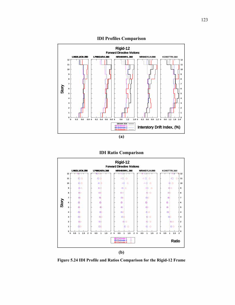
123
IDI Profiles Comparison
(a)
IDI Ratio Comparison
(b)
Figure 5.24 IDI Profile and Ratios Comparison for the Rigid-12 Frame
0
1
2
3
4
5
6
7
8
9
10
11
12
0 0.3 0.6 0.9
Rigid-12Forward Directive Motions
Sto
ry
Interstory Drift Index, (%)
LN92LUCN.250
DRAIN 2DXIDI Estimate 1IDI Estimate 2IDI Estimate 3
0 0.2 0.4 0.6 0.8
Rigid-12Forward Directive Motions
Sto
ry
Interstory Drift Index, (%)
LN92LUCN.250 LP89SARA.360
0 0.6 1.2 1.8
Rigid-12Forward Directive Motions
Sto
ry
Interstory Drift Index, (%)
LN92LUCN.250 LP89SARA.360 NR94NWHL.360
0 0.3 0.6 0.9 1.2
Rigid-12Forward Directive Motions
Sto
ry
Interstory Drift Index, (%)
LN92LUCN.250 LP89SARA.360 NR94NWHL.360 NR94SYLH.090
0 0.6 1.2 1.8 2.40
1
2
3
4
5
6
7
8
9
10
11
12
Rigid-12Forward Directive Motions
Sto
ry
Interstory Drift Index, (%)
LN92LUCN.250 LP89SARA.360 NR94NWHL.360 NR94SYLH.090 KO95TTRI.360
0
1
2
3
4
5
6
7
8
9
10
11
12
0 0.5 1 1.5 2
Rigid-12Forward Directive Motions
Sto
ry
Ratio
LN92LUCN.250
IDI Estimate 1IDI Estimate 2IDI Estimate 3
0 0.5 1 1.5 2
Rigid-12Forward Directive Motions
Sto
ry
Ratio
LN92LUCN.250 LP89SARA.360
0 0.5 1 1.5 2
Rigid-12Forward Directive Motions
Sto
ry
Ratio
LN92LUCN.250 LP89SARA.360 NR94NWHL.360
0 0.5 1 1.5 2
Rigid-12Forward Directive Motions
Sto
ry
Ratio
LN92LUCN.250 LP89SARA.360 NR94NWHL.360 NR94SYLH.090
0 0.5 1 1.5 20
1
2
3
4
5
6
7
8
9
10
11
12
Rigid-12Forward Directive Motions
Sto
ry
Ratio
LN92LUCN.250 LP89SARA.360 NR94NWHL.360 NR94SYLH.090 KO95TTRI.360
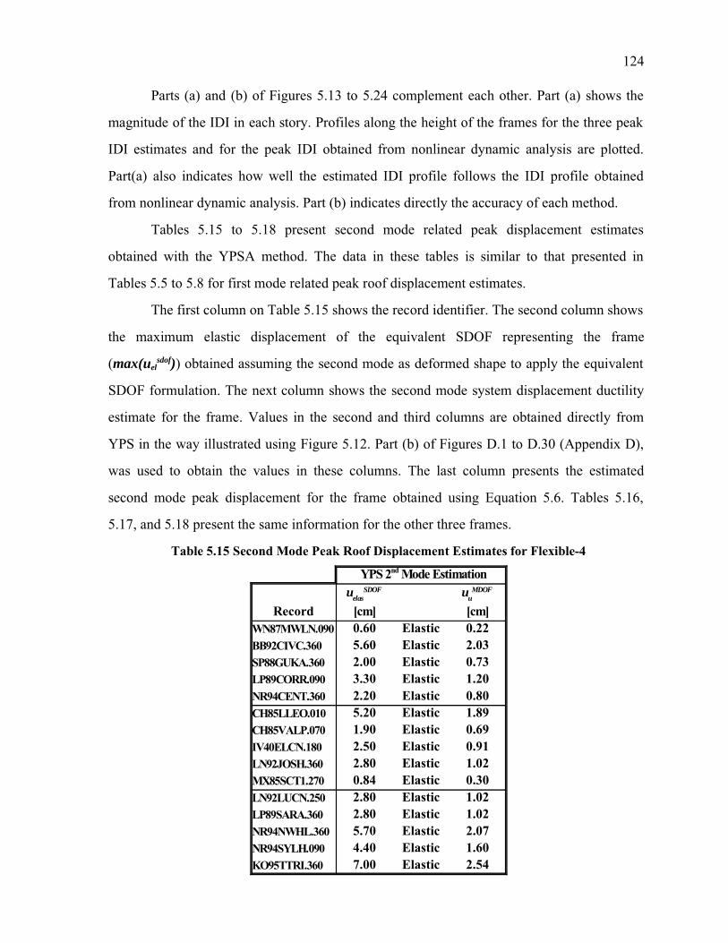
124
Parts (a) and (b) of Figures 5.13 to 5.24 complement each other. Part (a) shows the
magnitude of the IDI in each story. Profiles along the height of the frames for the three peak
IDI estimates and for the peak IDI obtained from nonlinear dynamic analysis are plotted.
Part(a) also indicates how well the estimated IDI profile follows the IDI profile obtained
from nonlinear dynamic analysis. Part (b) indicates directly the accuracy of each method.
Tables 5.15 to 5.18 present second mode related peak displacement estimates
obtained with the YPSA method. The data in these tables is similar to that presented in
Tables 5.5 to 5.8 for first mode related peak roof displacement estimates.
The first column on Table 5.15 shows the record identifier. The second column shows
the maximum elastic displacement of the equivalent SDOF representing the frame
(max(uelsdof)) obtained assuming the second mode as deformed shape to apply the equivalent
SDOF formulation. The next column shows the second mode system displacement ductility
estimate for the frame. Values in the second and third columns are obtained directly from
YPS in the way illustrated using Figure 5.12. Part (b) of Figures D.1 to D.30 (Appendix D),
was used to obtain the values in these columns. The last column presents the estimated
second mode peak displacement for the frame obtained using Equation 5.6. Tables 5.16,
5.17, and 5.18 present the same information for the other three frames.
Table 5.15 Second Mode Peak Roof Displacement Estimates for Flexible-4
Record æ0.60 Elastic 0.225.60 Elastic 2.032.00 Elastic 0.733.30 Elastic 1.202.20 Elastic 0.805.20 Elastic 1.891.90 Elastic 0.692.50 Elastic 0.912.80 Elastic 1.020.84 Elastic 0.302.80 Elastic 1.022.80 Elastic 1.025.70 Elastic 2.074.40 Elastic 1.607.00 Elastic 2.54
YPS 2nd Mode Estimationuelas
SDOF
[cm]uu
MDOF
[cm]WN87MWLN.090BB92CIVC.360SP88GUKA.360LP89CORR.090NR94CENT.360CH85LLEO.010CH85VALP.070IV40ELCN.180LN92JOSH.360MX85SCT1.270LN92LUCN.250LP89SARA.360NR94NWHL.360NR94SYLH.090KO95TTRI.360

125
Table 5.16 Second Mode Peak Roof Displacement Estimates for Rigid-4
Record æ0.38 Elastic 0.153.00 Elastic 1.200.90 Elastic 0.361.85 Elastic 0.740.85 Elastic 0.344.30 Elastic 1.720.75 Elastic 0.301.70 Elastic 0.681.00 Elastic 0.400.35 Elastic 0.142.20 Elastic 0.881.30 Elastic 0.523.40 Elastic 1.361.40 Elastic 0.562.00 Elastic 0.80
YPS 2nd Mode Estimationuelas
SDOF
[cm]uu
MDOF
[cm]WN87MWLN.090BB92CIVC.360SP88GUKA.360LP89CORR.090NR94CENT.360CH85LLEO.010CH85VALP.070IV40ELCN.180LN92JOSH.360MX85SCT1.270LN92LUCN.250LP89SARA.360NR94NWHL.360NR94SYLH.090KO95TTRI.360
Table 5.17 Second Mode Peak Roof Displacement Estimates for Flexible-12
Record æ0.51 Elastic 0.294.00 Elastic 2.273.20 Elastic 1.82
19.36 1.09 12.047.00 Elastic 3.98
19.36 Elastic 11.005.80 Elastic 3.30
10.00 Elastic 5.6812.20 Elastic 6.935.50 Elastic 3.13
10.70 Elastic 6.088.00 Elastic 4.55
19.36 1.30 14.3219.36 1.11 12.2419.36 1.56 17.14
YPS 2nd Mode Estimationuelas
SDOF
[cm]uu
MDOF
[cm]WN87MWLN.090BB92CIVC.360SP88GUKA.360LP89CORR.090NR94CENT.360CH85LLEO.010CH85VALP.070IV40ELCN.180LN92JOSH.360MX85SCT1.270LN92LUCN.250LP89SARA.360NR94NWHL.360NR94SYLH.090KO95TTRI.360

126
5.4.3.2 Analysis of Results
Some observations with respect to the accuracy of simplified equations used to
estimate interstory drift index can be pointed out with help from Figures 5.13 to 5.24 and
statistical analysis of the results. Tables 5.19 and 5.20 present statistics, for all the ground
motions, of the ratios between the peak interstory drift index estimates and the corresponding
value obtained from nonlinear dynamic analyses. Mean and standard deviations are shown
for the three IDI estimates.
For each frame, Table 5.19 shows the mean and standard deviation of the ratio of the
absolute peak IDI estimation to the absolute maximum IDI from the nonlinear dynamic
analyses, regardless of the story in which these two values occurred.
Table 5.18 Second Mode Peak Roof Displacement Estimates for Rigid-12
Record æ0.42 Elastic 0.2585.00 Elastic 3.0773.00 Elastic 1.8465.50 Elastic 3.3853.40 Elastic 2.092
10.50 Elastic 6.4613.80 Elastic 2.3385.50 Elastic 3.3854.70 Elastic 2.8921.60 Elastic 0.9853.70 Elastic 2.2773.70 Elastic 2.277
11.00 Elastic 6.7698.50 Elastic 5.231
11.00 Elastic 6.769
YPS 2nd Mode Estimationuelas
SDOF
[cm]uu
MDOF
[cm]WN87MWLN.090BB92CIVC.360SP88GUKA.360LP89CORR.090NR94CENT.360CH85LLEO.010CH85VALP.070IV40ELCN.180LN92JOSH.360MX85SCT1.270LN92LUCN.250LP89SARA.360NR94NWHL.360NR94SYLH.090KO95TTRI.360
Table 5.19 Ratio of Absolute Peak IDI Estimates to Peak IDI Computed inNonlinear Dynamic Analysis
IDI Estimate 1 IDI Estimate 2 IDI Estimate 3Mean Mean Mean
Flexible-4 0.905 0.134 0.926 0.090 1.081 0.101Rigid-4 0.912 0.137 0.958 0.080 1.131 0.090Flexible-12 0.570 0.200 0.755 0.158 1.002 0.220Rigid-12 0.695 0.203 0.847 0.141 1.139 0.181
Std. Dev. Std. Dev. Std. Dev.

127
For the 4-story frames, Table 5.19 shows that the mean results obtained using IDI
Estimate 1 (first mode shape and Equation 5.7) are good, although a little low compared to
results obtained from nonlinear dynamic analyses. Use of IDI Estimate 2 (two mode shapes
and Equation 5.8; SRSS) produces better mean estimates with significant reduction in the
dispersion of the results compared with IDI Estimate 1. Mean results from IDI Estimate 3
(two mode shapes and Equation 5.9; ABS Max) are also good for the 4-story building;
although, this equation overestimates mean results and has a larger standard deviation.
For the 12-story frames, Table 5.19 shows that the mean results obtained using IDI
Estimate 1 are significantly below the results obtained from nonlinear dynamic analyses with
a dispersion larger than the one obtained for the 4-story frames using the same equation. Use
of IDI Estimate 2 produces better mean estimates compared with IDI Estimate 1 but not as
good as the mean results obtained for the 4-story frames using the same equation. There was
a reduction in the dispersion of the results compared with IDI Estimate 1. Mean results from
IDI Estimate 3 are good for the 12-story building. This equation slightly overestimates mean
results and has larger dispersion compared with IDI Estimate 2.
Tables 5.20 and 5.21 show statistics, including results from all the ground motions,
for each individual story and all the stories collectively for the frames considered.
Table 5.20 Statistics of Story Ratios of Estimated IDI to Computed IDI for 4-Story Frames
Flexible-4
Rigid-4
IDI Estimate 1 IDI Estimate 2 IDI Estimate 3Story Mean Mean Mean
4 0.995 0.453 1.166 0.384 1.538 0.4583 0.999 0.264 1.056 0.219 1.285 0.2002 0.995 0.074 0.996 0.073 1.038 0.0691 0.888 0.142 0.929 0.126 1.115 0.177
Total 0.970 0.272 1.036 0.243 1.243 0.324
Std. Dev. Std. Dev. Std. Dev.
IDI Estimate 1 IDI Estimate 2 IDI Estimate 3Story Mean Mean Mean
4 0.871 0.239 0.983 0.154 1.250 0.1693 0.964 0.150 1.010 0.125 1.196 0.1592 1.006 0.069 1.012 0.064 1.089 0.0721 0.946 0.129 0.998 0.130 1.195 0.212
Total 0.947 0.162 1.001 0.120 1.182 0.168
Std. Dev. Std. Dev. Std. Dev.

128
Table 5.21 Statistics of Story Ratios of Estimated IDI to Computed IDI for 12-Story Frames
Flexible-12
Rigid-12
IDI Estimate 1 IDI Estimate 2 IDI Estimate 3Story Mean Mean Mean
12 0.440 0.236 0.781 0.233 1.048 0.31111 0.484 0.251 0.813 0.202 1.096 0.27210 0.575 0.244 0.881 0.173 1.197 0.2279 0.644 0.242 0.889 0.182 1.206 0.2118 0.704 0.233 0.856 0.202 1.140 0.2287 0.746 0.179 0.812 0.173 1.025 0.2056 0.811 0.123 0.817 0.123 0.894 0.1375 0.831 0.176 0.844 0.176 0.956 0.2044 0.831 0.202 0.893 0.194 1.125 0.2563 0.813 0.187 0.927 0.165 1.219 0.2402 0.804 0.188 0.955 0.147 1.276 0.2211 0.814 0.235 0.987 0.191 1.323 0.258
Total 0.708 0.245 0.871 0.186 1.126 0.259
Std. Dev. Std. Dev. Std. Dev.
IDI Estimate 1 IDI Estimate 2 IDI Estimate 3Story Mean Mean Mean
12 0.629 0.298 0.853 0.259 1.170 0.34411 0.690 0.256 0.915 0.188 1.252 0.23810 0.740 0.214 0.914 0.155 1.236 0.1879 0.788 0.189 0.906 0.149 1.196 0.1738 0.843 0.139 0.900 0.118 1.129 0.1337 0.881 0.128 0.896 0.122 1.027 0.1206 0.885 0.139 0.885 0.139 0.887 0.1385 0.895 0.122 0.905 0.119 1.015 0.1224 0.885 0.131 0.918 0.125 1.105 0.1573 0.890 0.135 0.947 0.131 1.186 0.1862 0.898 0.142 0.976 0.126 1.246 0.1771 0.891 0.155 0.979 0.133 1.263 0.181
Total 0.826 0.195 0.916 0.151 1.143 0.214
Std. Dev. Std. Dev. Std. Dev.

129
For the 4-story frames, Table 5.20 shows that the use of one mode to estimate
interstory drift indices (IDI Estimate 1) produces good mean results for all the stories of the
frames. While results for the second and third floor are very good in general, estimates for
the other stories are a little low. Mean results from IDI Estimate 2 may be considered to be
better than those of IDI Estimate 1. Additionally, there is reduction in the dispersion of the
results. In general, IDI Estimate 3 overestimates mean results for interstory drift indices, with
dispersions comparable to those obtained using IDI Estimate 1. Looking at the stories
collectively, IDI Estimate 1 underestimates mean results of interstory drift indices while IDI
Estimate 2 slightly overestimates them. The results of dispersion for IDI Estimate 2 was
lower than that for IDI Estimate 1. IDI Estimate 3 overestimates mean results of interstory
drift indices, and has larger dispersion compared with the other two estimates.
For the 12-story frames, Table 5.21 shows that mean results obtained using IDI
Estimate 1 and IDI Estimate 2 underestimate interstory drift indices for any individual story
of the frames. Although both underestimate interstory drift indices, estimates obtained using
IDI Estimate 2 are more accurate than those of IDI Estimate 1. The dispersion in the results
for IDI Estimate 2 was lower than that for IDI Estimate 1. In general, IDI Estimate 3
overestimates mean interstory drift indices, with larger dispersion compared with IDI
Estimate 1 and IDI Estimate 2.
IDI Estimate 2 is definitely better at the upper and lower stories of the frames
compared with IDI Estimate 1 and IDI Estimate 3, although the accuracy of the peak
interstory drift indices estimates was reduced towards the top of the frames for IDI Estimate
1 and IDI Estimate 2. On the other hand, IDI Estimate 3 produces better results toward the
center of the frame, and is less accurate at the lower stories.
For all the frames, Equation 5.8 (IDI Estimate 2) results in the lowest dispersion of all
the equations considered. In general, the dispersion associated with this estimate increases
towards the top and bottom stories of the frames, with greatest dispersion toward the top.
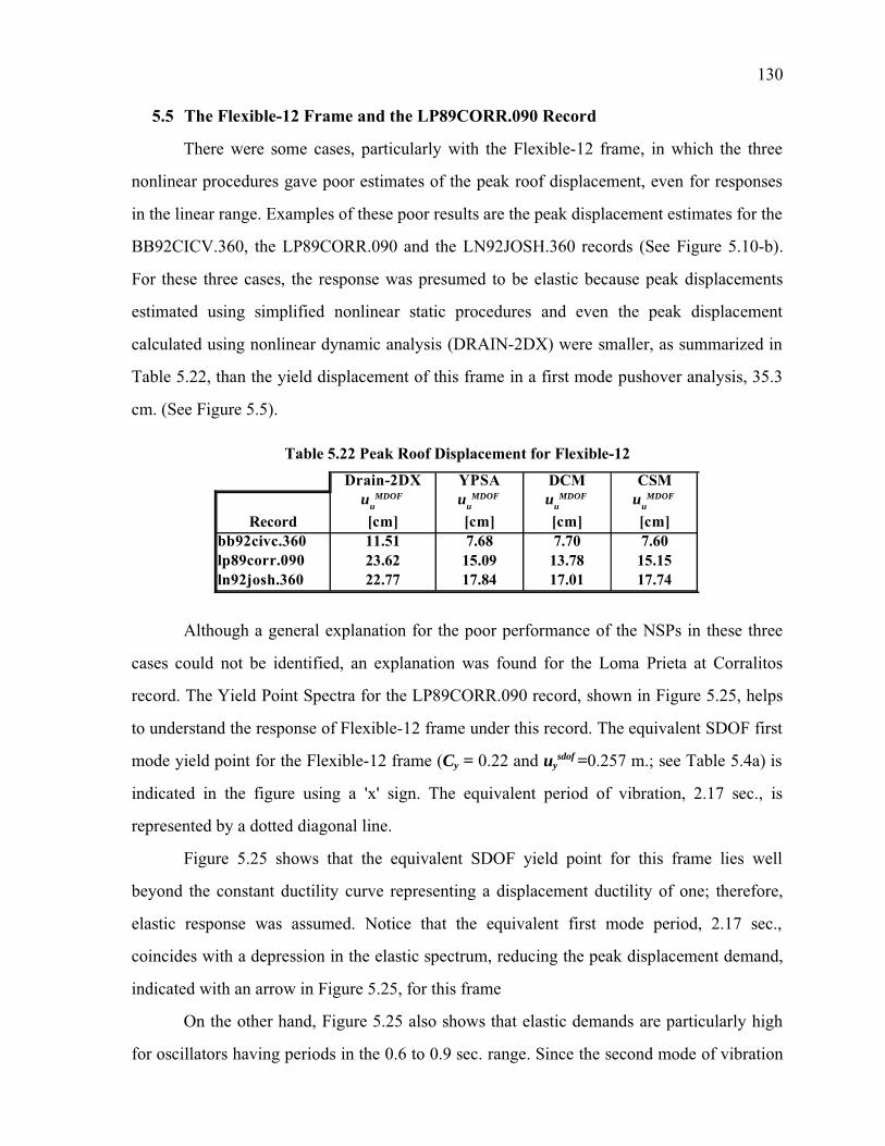
130
5.5 The Flexible-12 Frame and the LP89CORR.090 Record
There were some cases, particularly with the Flexible-12 frame, in which the three
nonlinear procedures gave poor estimates of the peak roof displacement, even for responses
in the linear range. Examples of these poor results are the peak displacement estimates for the
BB92CICV.360, the LP89CORR.090 and the LN92JOSH.360 records (See Figure 5.10-b).
For these three cases, the response was presumed to be elastic because peak displacements
estimated using simplified nonlinear static procedures and even the peak displacement
calculated using nonlinear dynamic analysis (DRAIN-2DX) were smaller, as summarized in
Table 5.22, than the yield displacement of this frame in a first mode pushover analysis, 35.3
cm. (See Figure 5.5).
Although a general explanation for the poor performance of the NSPs in these three
cases could not be identified, an explanation was found for the Loma Prieta at Corralitos
record. The Yield Point Spectra for the LP89CORR.090 record, shown in Figure 5.25, helps
to understand the response of Flexible-12 frame under this record. The equivalent SDOF first
mode yield point for the Flexible-12 frame (Cy = 0.22 and uysdof =0.257 m.; see Table 5.4a) is
indicated in the figure using a 'x' sign. The equivalent period of vibration, 2.17 sec., is
represented by a dotted diagonal line.
Figure 5.25 shows that the equivalent SDOF yield point for this frame lies well
beyond the constant ductility curve representing a displacement ductility of one; therefore,
elastic response was assumed. Notice that the equivalent first mode period, 2.17 sec.,
coincides with a depression in the elastic spectrum, reducing the peak displacement demand,
indicated with an arrow in Figure 5.25, for this frame
On the other hand, Figure 5.25 also shows that elastic demands are particularly high
for oscillators having periods in the 0.6 to 0.9 sec. range. Since the second mode of vibration
Table 5.22 Peak Roof Displacement for Flexible-12
DCM CSM
Record11.51 7.68 7.70 7.6023.62 15.09 13.78 15.1522.77 17.84 17.01 17.74
Drain-2DX YPSAuu
MDOF
[cm]uu
MDOF
[cm]uu
MDOF
[cm]uu
MDOF
[cm]bb92civc.360lp89corr.090ln92josh.360

131
of the Flexible-12 frame has a period of 0.80 sec. (Table 5.4b), it was considered that the
response of Flexible-12 frame to this record may have been significantly influenced by the
second mode of vibration.
Figure 5.26 shows the Yield Point Spectra for the LP89CORR.090 record generated
using damping equal to 2.8%. In this figure, the equivalent SDOF second mode yield point
for the Flexible-12 frame (Cy = 1.2 and uysdof = 0.19 m.; see Table 5.4b) is indicated with a 'x'
sign. This figure shows that the second mode period of the Flexible-12 frame was very
excited. Even more, the figure suggests that some nonlinear behavior occurs in the frame
because the yield point for the second mode lies between the curves of displacement
ductilities 1 and 2.
The YPS estimate for the peak roof displacement using the first mode of vibration for
this record is 15.1 cm. (see Table 5.7) while a similar estimate for the second mode is 12.04
cm. (see Table 5.17). The peak roof displacement estimate for second mode represents a 80%
of that due to the first mode. The mean for this ratio considering the 15 ground motion was
28% for this frame, confirming the high influence of the second mode in the response of this
frame to the Loma Prieta at Corralitos record.
Figure 5.25 5% Damped Yield Point Spectra for Loma Prieta at Corralitos
The 'x' Sign Indicates the First Mode Yield Point of the Flexible-12 Frame
1Ε−03
1Ε−02
1Ε−01
1Ε+00
1Ε−04 1Ε−03 1Ε−02 1Ε−01 1Ε+00
Bilinear for LP89CORR.090, 5% Damping, 10% Post Yield Stiffness
Yie
ld S
tren
gth
Coe
ffici
ent (
C )y
Yield Displacement, (m)
xT= 0.05
T= 0.1
T= 1.0 T= 10.0
µ=1µ=2µ=4µ=8
1Ε−03
1Ε−02
1Ε−01
1Ε+00
1Ε−04 1Ε−03 1Ε−02 1Ε−01 1Ε+00
Bilinear for LP89CORR.090, 5% Damping, 10% Post Yield Stiffness
Yie
ld S
tren
gth
Coe
ffici
ent (
C )y
Yield Displacement, (m)
xT= 0.05
T= 0.1
T= 1.0 T= 10.01Ε−03
1Ε−02
1Ε−01
1Ε+00
1Ε−04 1Ε−03 1Ε−02 1Ε−01 1Ε+00
Bilinear for LP89CORR.090, 5% Damping, 10% Post Yield Stiffness
Yie
ld S
tren
gth
Coe
ffici
ent (
C )y
Yield Displacement, (m)
xT= 0.05
T= 0.1
T= 1.0 T= 10.01Ε−03
1Ε−02
1Ε−01
1Ε+00
1Ε−04 1Ε−03 1Ε−02 1Ε−01 1Ε+00
Bilinear for LP89CORR.090, 5% Damping, 10% Post Yield Stiffness
Yie
ld S
tren
gth
Coe
ffici
ent (
C )y
Yield Displacement, (m)
xT= 0.05
T= 0.1
T= 1.0 T= 10.01Ε−03
1Ε−02
1Ε−01
1Ε+00
1Ε−04 1Ε−03 1Ε−02 1Ε−01 1Ε+00
Bilinear for LP89CORR.090, 5% Damping, 10% Post Yield Stiffness
Yie
ld S
tren
gth
Coe
ffici
ent (
C )y
Yield Displacement, (m)
xT= 0.05
T= 0.1
T= 1.0 T= 10.01Ε−03
1Ε−02
1Ε−01
1Ε+00
1Ε−04 1Ε−03 1Ε−02 1Ε−01 1Ε+00
Bilinear for LP89CORR.090, 5% Damping, 10% Post Yield Stiffness
Yie
ld S
tren
gth
Coe
ffici
ent (
C )y
Yield Displacement, (m)
xT= 0.05
T= 0.1
T= 1.0 T= 10.01Ε−03
1Ε−02
1Ε−01
1Ε+00
1Ε−04 1Ε−03 1Ε−02 1Ε−01 1Ε+00
Bilinear for LP89CORR.090, 5% Damping, 10% Post Yield Stiffness
Yie
ld S
tren
gth
Coe
ffici
ent (
C )y
Yield Displacement, (m)
xT= 0.05
T= 0.1
T= 1.0 T= 10.01Ε−03
1Ε−02
1Ε−01
1Ε+00
1Ε−04 1Ε−03 1Ε−02 1Ε−01 1Ε+00
Bilinear for LP89CORR.090, 5% Damping, 10% Post Yield Stiffness
Yie
ld S
tren
gth
Coe
ffici
ent (
C )y
Yield Displacement, (m)
xT= 0.05
T= 0.1
T= 1.0 T= 10.01Ε−03
1Ε−02
1Ε−01
1Ε+00
1Ε−04 1Ε−03 1Ε−02 1Ε−01 1Ε+00
Bilinear for LP89CORR.090, 5% Damping, 10% Post Yield Stiffness
Yie
ld S
tren
gth
Coe
ffici
ent (
C )y
Yield Displacement, (m)
xT= 0.05
T= 0.1
T= 1.0 T= 10.01Ε−03
1Ε−02
1Ε−01
1Ε+00
1Ε−04 1Ε−03 1Ε−02 1Ε−01 1Ε+00
Bilinear for LP89CORR.090, 5% Damping, 10% Post Yield Stiffness
Yie
ld S
tren
gth
Coe
ffici
ent (
C )y
Yield Displacement, (m)
xT= 0.05
T= 0.1
T= 1.0 T= 10.01Ε−03
1Ε−02
1Ε−01
1Ε+00
1Ε−04 1Ε−03 1Ε−02 1Ε−01 1Ε+00
Bilinear for LP89CORR.090, 5% Damping, 10% Post Yield Stiffness
Yie
ld S
tren
gth
Coe
ffici
ent (
C )y
Yield Displacement, (m)
xT= 0.05
T= 0.1
T= 1.0 T= 10.01Ε−03
1Ε−02
1Ε−01
1Ε+00
1Ε−04 1Ε−03 1Ε−02 1Ε−01 1Ε+00
Bilinear for LP89CORR.090, 5% Damping, 10% Post Yield Stiffness
Yie
ld S
tren
gth
Coe
ffici
ent (
C )y
Yield Displacement, (m)
xT= 0.05
T= 0.1
T= 1.0 T= 10.01Ε−03
1Ε−02
1Ε−01
1Ε+00
1Ε−04 1Ε−03 1Ε−02 1Ε−01 1Ε+00
Bilinear for LP89CORR.090, 5% Damping, 10% Post Yield Stiffness
Yie
ld S
tren
gth
Coe
ffici
ent (
C )y
Yield Displacement, (m)
xT= 0.05
T= 0.1
T= 1.0 T= 10.01Ε−03
1Ε−02
1Ε−01
1Ε+00
1Ε−04 1Ε−03 1Ε−02 1Ε−01 1Ε+00
Bilinear for LP89CORR.090, 5% Damping, 10% Post Yield Stiffness
Yie
ld S
tren
gth
Coe
ffici
ent (
C )y
Yield Displacement, (m)
xT= 0.05
T= 0.1
T= 1.0 T= 10.01Ε−03
1Ε−02
1Ε−01
1Ε+00
1Ε−04 1Ε−03 1Ε−02 1Ε−01 1Ε+00
Bilinear for LP89CORR.090, 5% Damping, 10% Post Yield Stiffness
Yie
ld S
tren
gth
Coe
ffici
ent (
C )y
Yield Displacement, (m)
xT= 0.05
T= 0.1
T= 1.0 T= 10.01Ε−03
1Ε−02
1Ε−01
1Ε+00
1Ε−04 1Ε−03 1Ε−02 1Ε−01 1Ε+00
Bilinear for LP89CORR.090, 5% Damping, 10% Post Yield Stiffness
Yie
ld S
tren
gth
Coe
ffici
ent (
C )y
Yield Displacement, (m)
xT= 0.05
T= 0.1
T= 1.0 T= 10.01Ε−03
1Ε−02
1Ε−01
1Ε+00
1Ε−04 1Ε−03 1Ε−02 1Ε−01 1Ε+00
Bilinear for LP89CORR.090, 5% Damping, 10% Post Yield Stiffness
Yie
ld S
tren
gth
Coe
ffici
ent (
C )y
Yield Displacement, (m)
xT= 0.05
T= 0.1
T= 1.0 T= 10.01Ε−03
1Ε−02
1Ε−01
1Ε+00
1Ε−04 1Ε−03 1Ε−02 1Ε−01 1Ε+00
Bilinear for LP89CORR.090, 5% Damping, 10% Post Yield Stiffness
Yie
ld S
tren
gth
Coe
ffici
ent (
C )y
Yield Displacement, (m)
xT= 0.05
T= 0.1
T= 1.0 T= 10.01Ε−03
1Ε−02
1Ε−01
1Ε+00
1Ε−04 1Ε−03 1Ε−02 1Ε−01 1Ε+00
Bilinear for LP89CORR.090, 5% Damping, 10% Post Yield Stiffness
Yie
ld S
tren
gth
Coe
ffici
ent (
C )y
Yield Displacement, (m)
xT= 0.05
T= 0.1
T= 1.0 T= 10.01Ε−03
1Ε−02
1Ε−01
1Ε+00
1Ε−04 1Ε−03 1Ε−02 1Ε−01 1Ε+00
Bilinear for LP89CORR.090, 5% Damping, 10% Post Yield Stiffness
Yie
ld S
tren
gth
Coe
ffici
ent (
C )y
Yield Displacement, (m)
xT= 0.05
T= 0.1
T= 1.0 T= 10.01Ε−03
1Ε−02
1Ε−01
1Ε+00
1Ε−04 1Ε−03 1Ε−02 1Ε−01 1Ε+00
Bilinear for LP89CORR.090, 5% Damping, 10% Post Yield Stiffness
Yie
ld S
tren
gth
Coe
ffici
ent (
C )y
Yield Displacement, (m)
xT= 0.05
T= 0.1
T= 1.0 T= 10.01Ε−03
1Ε−02
1Ε−01
1Ε+00
1Ε−04 1Ε−03 1Ε−02 1Ε−01 1Ε+00
Bilinear for LP89CORR.090, 5% Damping, 10% Post Yield Stiffness
Yie
ld S
tren
gth
Coe
ffici
ent (
C )y
Yield Displacement, (m)
xT= 0.05
T= 0.1
T= 1.0 T= 10.0

132
Analysis using DRAIN-2DX confirmed that nonlinear behavior occurs in this frame
during its response to the LP89CORR.090 record.
Figure 5.27 shows plastic hinges formed in Flexible-12 frame after being subjected to
the Loma Prieta at Corralitos record. A total of 36 plastic hinges were produced by this
record, 32 beam hinges and 4 column hinges. Plastic hinges are shown as dark circles. This
figure confirms that the Flexible-12 frame experienced nonlinear deformations responding to
the LP89CORR.090 record.
Figure 5.26 2.8% Damped Yield Point Spectra for Loma Prieta at Corralitos
The 'x' Sign Indicates the Second Mode Yield Point of the Flexible-12 Frame
1Ε−03
1Ε−02
1Ε−01
1Ε+00
1Ε−04 1Ε−03 1Ε−02 1Ε−01 1Ε+00
Bilinear for LP89CORR.090, 2.8% Damping, 10% Post Yield Stiffness
Yie
ld S
tren
gth
Coe
ffici
ent (
C )y
Yield Displacement, (m)
x
T= 0.05
T= 0.1
T= 1.0 T= 10.0µ=1µ=2
1Ε−03
1Ε−02
1Ε−01
1Ε+00
1Ε−04 1Ε−03 1Ε−02 1Ε−01 1Ε+00
Bilinear for LP89CORR.090, 2.8% Damping, 10% Post Yield Stiffness
Yie
ld S
tren
gth
Coe
ffici
ent (
C )y
Yield Displacement, (m)
x
T= 0.05
T= 0.1
T= 1.0 T= 10.01Ε−03
1Ε−02
1Ε−01
1Ε+00
1Ε−04 1Ε−03 1Ε−02 1Ε−01 1Ε+00
Bilinear for LP89CORR.090, 2.8% Damping, 10% Post Yield Stiffness
Yie
ld S
tren
gth
Coe
ffici
ent (
C )y
Yield Displacement, (m)
x
T= 0.05
T= 0.1
T= 1.0 T= 10.01Ε−03
1Ε−02
1Ε−01
1Ε+00
1Ε−04 1Ε−03 1Ε−02 1Ε−01 1Ε+00
Bilinear for LP89CORR.090, 2.8% Damping, 10% Post Yield Stiffness
Yie
ld S
tren
gth
Coe
ffici
ent (
C )y
Yield Displacement, (m)
x
T= 0.05
T= 0.1
T= 1.0 T= 10.01Ε−03
1Ε−02
1Ε−01
1Ε+00
1Ε−04 1Ε−03 1Ε−02 1Ε−01 1Ε+00
Bilinear for LP89CORR.090, 2.8% Damping, 10% Post Yield Stiffness
Yie
ld S
tren
gth
Coe
ffici
ent (
C )y
Yield Displacement, (m)
x
T= 0.05
T= 0.1
T= 1.0 T= 10.01Ε−03
1Ε−02
1Ε−01
1Ε+00
1Ε−04 1Ε−03 1Ε−02 1Ε−01 1Ε+00
Bilinear for LP89CORR.090, 2.8% Damping, 10% Post Yield Stiffness
Yie
ld S
tren
gth
Coe
ffici
ent (
C )y
Yield Displacement, (m)
x
T= 0.05
T= 0.1
T= 1.0 T= 10.01Ε−03
1Ε−02
1Ε−01
1Ε+00
1Ε−04 1Ε−03 1Ε−02 1Ε−01 1Ε+00
Bilinear for LP89CORR.090, 2.8% Damping, 10% Post Yield Stiffness
Yie
ld S
tren
gth
Coe
ffici
ent (
C )y
Yield Displacement, (m)
x
T= 0.05
T= 0.1
T= 1.0 T= 10.01Ε−03
1Ε−02
1Ε−01
1Ε+00
1Ε−04 1Ε−03 1Ε−02 1Ε−01 1Ε+00
Bilinear for LP89CORR.090, 2.8% Damping, 10% Post Yield Stiffness
Yie
ld S
tren
gth
Coe
ffici
ent (
C )y
Yield Displacement, (m)
x
T= 0.05
T= 0.1
T= 1.0 T= 10.01Ε−03
1Ε−02
1Ε−01
1Ε+00
1Ε−04 1Ε−03 1Ε−02 1Ε−01 1Ε+00
Bilinear for LP89CORR.090, 2.8% Damping, 10% Post Yield Stiffness
Yie
ld S
tren
gth
Coe
ffici
ent (
C )y
Yield Displacement, (m)
x
T= 0.05
T= 0.1
T= 1.0 T= 10.01Ε−03
1Ε−02
1Ε−01
1Ε+00
1Ε−04 1Ε−03 1Ε−02 1Ε−01 1Ε+00
Bilinear for LP89CORR.090, 2.8% Damping, 10% Post Yield Stiffness
Yie
ld S
tren
gth
Coe
ffici
ent (
C )y
Yield Displacement, (m)
x
T= 0.05
T= 0.1
T= 1.0 T= 10.01Ε−03
1Ε−02
1Ε−01
1Ε+00
1Ε−04 1Ε−03 1Ε−02 1Ε−01 1Ε+00
Bilinear for LP89CORR.090, 2.8% Damping, 10% Post Yield Stiffness
Yie
ld S
tren
gth
Coe
ffici
ent (
C )y
Yield Displacement, (m)
x
T= 0.05
T= 0.1
T= 1.0 T= 10.01Ε−03
1Ε−02
1Ε−01
1Ε+00
1Ε−04 1Ε−03 1Ε−02 1Ε−01 1Ε+00
Bilinear for LP89CORR.090, 2.8% Damping, 10% Post Yield Stiffness
Yie
ld S
tren
gth
Coe
ffici
ent (
C )y
Yield Displacement, (m)
x
T= 0.05
T= 0.1
T= 1.0 T= 10.01Ε−03
1Ε−02
1Ε−01
1Ε+00
1Ε−04 1Ε−03 1Ε−02 1Ε−01 1Ε+00
Bilinear for LP89CORR.090, 2.8% Damping, 10% Post Yield Stiffness
Yie
ld S
tren
gth
Coe
ffici
ent (
C )y
Yield Displacement, (m)
x
T= 0.05
T= 0.1
T= 1.0 T= 10.01Ε−03
1Ε−02
1Ε−01
1Ε+00
1Ε−04 1Ε−03 1Ε−02 1Ε−01 1Ε+00
Bilinear for LP89CORR.090, 2.8% Damping, 10% Post Yield Stiffness
Yie
ld S
tren
gth
Coe
ffici
ent (
C )y
Yield Displacement, (m)
x
T= 0.05
T= 0.1
T= 1.0 T= 10.01Ε−03
1Ε−02
1Ε−01
1Ε+00
1Ε−04 1Ε−03 1Ε−02 1Ε−01 1Ε+00
Bilinear for LP89CORR.090, 2.8% Damping, 10% Post Yield Stiffness
Yie
ld S
tren
gth
Coe
ffici
ent (
C )y
Yield Displacement, (m)
x
T= 0.05
T= 0.1
T= 1.0 T= 10.01Ε−03
1Ε−02
1Ε−01
1Ε+00
1Ε−04 1Ε−03 1Ε−02 1Ε−01 1Ε+00
Bilinear for LP89CORR.090, 2.8% Damping, 10% Post Yield Stiffness
Yie
ld S
tren
gth
Coe
ffici
ent (
C )y
Yield Displacement, (m)
x
T= 0.05
T= 0.1
T= 1.0 T= 10.01Ε−03
1Ε−02
1Ε−01
1Ε+00
1Ε−04 1Ε−03 1Ε−02 1Ε−01 1Ε+00
Bilinear for LP89CORR.090, 2.8% Damping, 10% Post Yield Stiffness
Yie
ld S
tren
gth
Coe
ffici
ent (
C )y
Yield Displacement, (m)
x
T= 0.05
T= 0.1
T= 1.0 T= 10.01Ε−03
1Ε−02
1Ε−01
1Ε+00
1Ε−04 1Ε−03 1Ε−02 1Ε−01 1Ε+00
Bilinear for LP89CORR.090, 2.8% Damping, 10% Post Yield Stiffness
Yie
ld S
tren
gth
Coe
ffici
ent (
C )y
Yield Displacement, (m)
x
T= 0.05
T= 0.1
T= 1.0 T= 10.01Ε−03
1Ε−02
1Ε−01
1Ε+00
1Ε−04 1Ε−03 1Ε−02 1Ε−01 1Ε+00
Bilinear for LP89CORR.090, 2.8% Damping, 10% Post Yield Stiffness
Yie
ld S
tren
gth
Coe
ffici
ent (
C )y
Yield Displacement, (m)
x
T= 0.05
T= 0.1
T= 1.0 T= 10.01Ε−03
1Ε−02
1Ε−01
1Ε+00
1Ε−04 1Ε−03 1Ε−02 1Ε−01 1Ε+00
Bilinear for LP89CORR.090, 2.8% Damping, 10% Post Yield Stiffness
Yie
ld S
tren
gth
Coe
ffici
ent (
C )y
Yield Displacement, (m)
x
T= 0.05
T= 0.1
T= 1.0 T= 10.01Ε−03
1Ε−02
1Ε−01
1Ε+00
1Ε−04 1Ε−03 1Ε−02 1Ε−01 1Ε+00
Bilinear for LP89CORR.090, 2.8% Damping, 10% Post Yield Stiffness
Yie
ld S
tren
gth
Coe
ffici
ent (
C )y
Yield Displacement, (m)
x
T= 0.05
T= 0.1
T= 1.0 T= 10.01Ε−03
1Ε−02
1Ε−01
1Ε+00
1Ε−04 1Ε−03 1Ε−02 1Ε−01 1Ε+00
Bilinear for LP89CORR.090, 2.8% Damping, 10% Post Yield Stiffness
Yie
ld S
tren
gth
Coe
ffici
ent (
C )y
Yield Displacement, (m)
x
T= 0.05
T= 0.1
T= 1.0 T= 10.0

133
Figure 5.27 Plastic Hinges Formed During Response to the Corralitos Record
3 @ 8.00 m.
4.00 m
4.00 m
4.00 m
4.00 m
4.00 m
4.00 m
4.00 m
4.00 m
4.00 m
4.00 m
4.00 m
5.00 m

134
5.6 Summary
A method to estimate peak displacement of multistory buildings was introduced, and
was identified as the YPSA method to differentiate it from the YPS design methodology
presented in Chapter 4. The YPSA method was classified as a nonlinear static procedure
(NSP).
Peak displacement estimates were obtained with three NSPs (the Displacement
Coefficient Method, the Capacity Spectrum Method and the YPSA method) and compared
using plots and tables. Mean and standard deviation statistics for the three NSPs were shown
and discussed.
Peak displacements corresponding to the second mode of vibration were obtained
using the YPSA method. These second mode related peak displacements and corresponding
values obtained for the first mode were combined to estimate interstory drift indices (IDI).
Results of the three IDI estimates are compared using plots, tables and simple statistics.
A special case in which the second mode causes significant yielding in one of the
frames analyzed was detected. For this particular case, the YPSA method was able to predict
the second mode related nonlinear behavior of the frame.
135
CHAPTER 6
SUMMARY AND CONCLUSIONS
6.1 Summary and Conclusions
This chapter summarizes the results obtained during the course of this study in
relation to three main objectives.
The first objective was to explore the utility of a new representation of constant
ductility response spectra named Yield Point Spectra (YPS). These spectra were used directly
for the design and analysis of SDOF structures. For design, graphical procedures were used
to determine combinations of strength and stiffness to limit drift and displacement ductility
demands to prescribed values. For analysis, accurate estimates of the the peak displacement
and displacement ductility demands of the SDOF structures were obtained using the
logarithmic form of YPS. An application of YPS to the performance-based design of a SDOF
structure was illustrated with an example. Yield Point Spectra for 15 ground motion records
and two load-deformation models were presented.
The second objective was to outline a design methodology for the seismic design of
regular multistory buildings using Yield Point Spectra. The methodology was formulated to
be as similar to current code approaches as possible. A minimum base shear strength for
design was determined based on user specified limits on peak roof displacement and
interstory drift. In contrast to current code approaches, which rely on an estimated period of
vibration, the proposed methodology uses an estimated yield displacement of the frame as the
initial parameter for seismic design. The methodology was illustrated by designing four
moment-resistant steel frames. The effectiveness of the methodology to limit peak roof
displacement and interstory drift was validated using nonlinear static and dynamic analyses.
The third objective was to develop a method in which YPS are used to estimate peak
displacement response and interstory drift of multistory frames. The method was identified as
the YPSA method, and classified as a Nonlinear Static Procedure (NSP). The YPSA method
was compared with others NSPs and with results from nonlinear dynamic analyses. The
YPSA method was also used to estimate interstory drift indices (IDI) using deformed shapes
of the frames based on the first mode and combinations of the first and second mode shapes.
136
The second and third objectives relate to the analysis and design of multistory
buildings. To achieve these objectives it was necessary to transform the multistory building
response to an equivalent SDOF system using established techniques. For the transformation,
the equivalent SDOF methodology requires the assumption of a deformed shape. For design
of the four case study frames, the deformed shape assumed had a triangular distribution of
lateral deflections. For the analysis of the frames, the assumed deformed shape was the first
elastic mode shape.
Finally, a peculiar case was identified in which the YPSA method detected the
nonlinear response in the second mode of vibration of one of the case study frames.
Based on the observations and analyses of results obtained from the set of four frames
and the fifteen ground motions considered in this study, the following conclusions and trends
were identified:
(1) Yield Point Spectra are useful for the analysis and design of SDOF systems. Yield Point
Spectra allow one to estimate the peak displacement and the displacement ductility
demands of SDOF structures. These spectra are also useful for establishing combinations
of strength and stiffness required to limit drift and displacement ductility demands to
arbitrary values.
(2) Yield Point Spectra provide a graphical approach to consider multiple performance levels
in performance-base seismic design. Individual YPS, representing a given intensity of
ground shaking and recurrence interval, may be used to define an admissible design region
conforming to specific performance levels. Two or more of these admissible design
regions may be superimposed to define a final design region according to the performance
objective.
(3) The equivalent SDOF methodology is useful for modeling the response of multistory
framed structures. The methodology permits analysis and design of multistory systems
using the Yield Point Spectra developed for SDOF oscillators.

137
(4) The proposed YPS design methodology was shown to be effective for limiting the peak
displacement response and interstory drift of the four example frames to the intended
values
(5) The use of yield displacement as an alternative to period as fundamental parameter for
seismic design seems feasible. For the four frames designed using this assumption, the
ratio of yield displacement to building height was within the suggested range (0.6%-
0.9%). Values of the yield displacement varied from 0.68% to 0.79% of the building
height for the four frames, while the fundamental period of vibration varied from 0.71 to
1.16 sec. for the 4-story frames and from 1.25 to 2.17 sec. for the 12-story frames.
(6) In general, buildings require a minimum lateral strength to control inelastic response
demands. The procedure used to provide the four example frames with the required
minimum strength was very effective. The procedure consists in obtaining preliminary
sizes for the structural members based on the design forces prescribed by the proposed
design methodology. After that, the design is refined using the approximate value of the
equivalent period (Equation 2.2) as a target to be matched by the actual first mode period
of the frame. If this observation, which is a consequence of the stability of the yield
displacement, is confirmed by future studies, then to provide a moment-resistant steel
frame with the required strength it would be sufficient to give it a fundamental period
equal or less than the equivalent period obtained from Yield Point Spectra. Furthermore,
the nonlinear static analysis (pushover) would be dispensable as a tool to verify the
strength of moment resistant steel frames. This observation also would be very useful for
all Nonlinear Static Procedures (NSPs).
(7) Approximate deformed shapes, in particular the triangular shape assumed to apply the
equivalent SDOF formulation to design the case study frames, appear to be adequate for
framed buildings. Although the other two parabolic deformed shapes were not used, they
may be appropriate for different building systems.
138
(8) Peak displacement estimates given by the YPSA method, the Displacement Coefficient
Method (DCM) and the Capacity Spectrum Method (CSM) were compared for the four
case-study frames. In a mean sense, results from the YPSA method and from the CSM are
similar although the YPSA method gave slightly more accurate mean estimates for the
four frames and 15 ground motions. The dispersion of the peak displacement estimates
using the YPSA method was smaller than the dispersion obtained using the CSM for the
four frames and 15 ground motions. The DCM overestimated mean results of the peak
displacements and had greater results in dispersion than the other two methods.
(9) Even though the CSM and the YPSA methods provide similar accuracy for estimating
peak displacement response, the simplicity of the YPSA method makes it more attractive.
In the YPSA method, peak displacement estimates are obtained by simply "reading"
system displacement ductility and maximum elastic displacement from the Yield Point
Spectra. In the CSM, peak displacement estimates are obtained using a more elaborate
iterative process.
(10) In general, interstory drift index estimates were less accurate then peak roof
displacement estimates.
(11) Peak roof displacements can be estimated using linear static analysis and the design
lateral forces obtained by distributing the base shear strength along the height of the
building. Ultimate roof displacement is obtained by multiplying displacements computed
under the design lateral forces by the system ductility demand read from YPS. However, a
similar procedure underestimates values for interstory drift indices.
(12) Profiles of interstory drift obtained using one deformed shape (fundamental mode shape)
amplified by the peak roof displacement, in a mean sense, provided good interstory drift
estimates for the 4-story frames; although, the dispersion of these estimates was a little
high. For the 12-story frames, the use of a single deformed shape was inadequate for good
interstory drift estimates. The inclusion of a second mode shape, combined with the
139
fundamental mode shape using the SRSS rule, to obtain interstory drift indices improves
the estimates and reduces their dispersion.
(13) The accuracy of peak roof displacements and interstory drift indices estimated using the
YPSA method show no particular tendency with respect to the three ground motion
categories: short duration, long duration and forward directivity.
6.2 Suggestions for Future Research
This research provides a basic framework for a methodology for the seismic design of
regular framed buildings. However, some issues remain unresolved and should be addressed
before the proposed methods may be generally recommended. Some of these are:
1) Yield Displacement Stability. It was shown that the ratio of the yield displacement to the
building height for moment resistant frames is very stable. This ratio and its stability
should be addressed for other structural systems such as reinforced concrete moment
frames and shear walls.
2) Smoothed Yield Point Spectra. Current code provisions prescribe smoothed design
spectra for design of building structures. The effectiveness of smoothed YPS constructed
from elastic spectra reduced using period-dependent strength reduction factors should be
verified.
3) Irregular Buildings. The proposed methodologies were effective controlling the peak roof
displacement and interstory drift of regular frame structures. The accuracy of the
methodologies addressing the same parameters in irregular buildings should be addressed.
Irregularities in mass distribution and soft stories should be studied.

140
APPENDIX A
SELECTED GROUND MOTIONS
Figures A.1 to A.15 presents detailed plots of the ground motion selected for this
study. These ground motion are listed in Table 2.2.
Each figure contain plots presenting time series data corresponding to the
acceleration, velocity and displacement for the record. Additionally, equivalent velocity
spectra and pseudo-acceleration spectra are also shown. These spectra were used to establish
the characteristic periods of the ground motions.
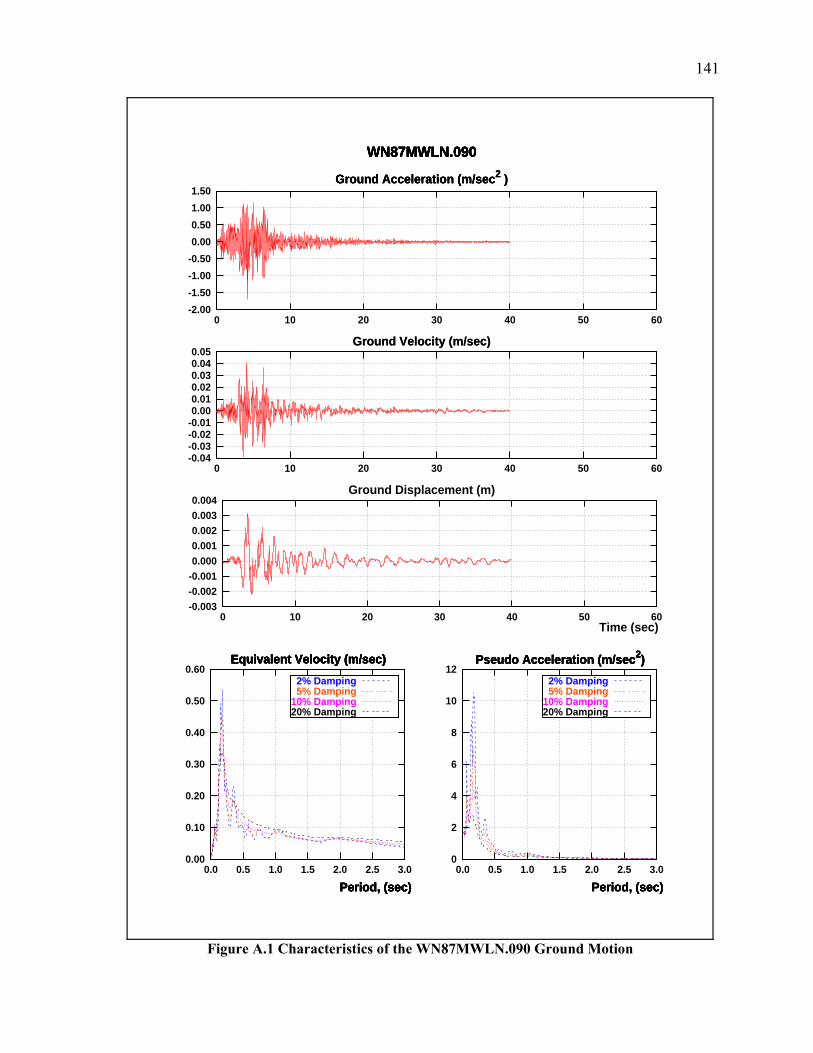
141
Figure A.1 Characteristics of the WN87MWLN.090 Ground Motion
0.00
0.10
0.20
0.30
0.40
0.50
0.60
0.0 0.5 1.0 1.5 2.0 2.5 3.0
WN87MWLN.090
Equivalent Velocity (m/sec)
Period, (sec)
2% Damping 5% Damping10% Damping20% Damping
0
2
4
6
8
10
12
0.0 0.5 1.0 1.5 2.0 2.5 3.0
WN87MWLN.090
Equivalent Velocity (m/sec)
Period, (sec)
Pseudo Acceleration (m/sec2)
Period, (sec)
2% Damping 5% Damping10% Damping20% Damping
-2.00
-1.50
-1.00
-0.50
0.00
0.50
1.00
1.50
0 10 20 30 40 50 60
WN87MWLN.090
Equivalent Velocity (m/sec)
Period, (sec)
Pseudo Acceleration (m/sec2)
Period, (sec)
Ground Acceleration (m/sec2 )
-0.04-0.03-0.02-0.010.000.010.020.030.040.05
0 10 20 30 40 50 60
WN87MWLN.090
Equivalent Velocity (m/sec)
Period, (sec)
Pseudo Acceleration (m/sec2)
Period, (sec)
Ground Acceleration (m/sec2 )
Ground Velocity (m/sec)
-0.003-0.002-0.0010.0000.0010.0020.0030.004
0 10 20 30 40 50 60
WN87MWLN.090
Equivalent Velocity (m/sec)
Period, (sec)
Pseudo Acceleration (m/sec2)
Period, (sec)
Ground Acceleration (m/sec2 )
Ground Velocity (m/sec)
Ground Displacement (m)
Time (sec)
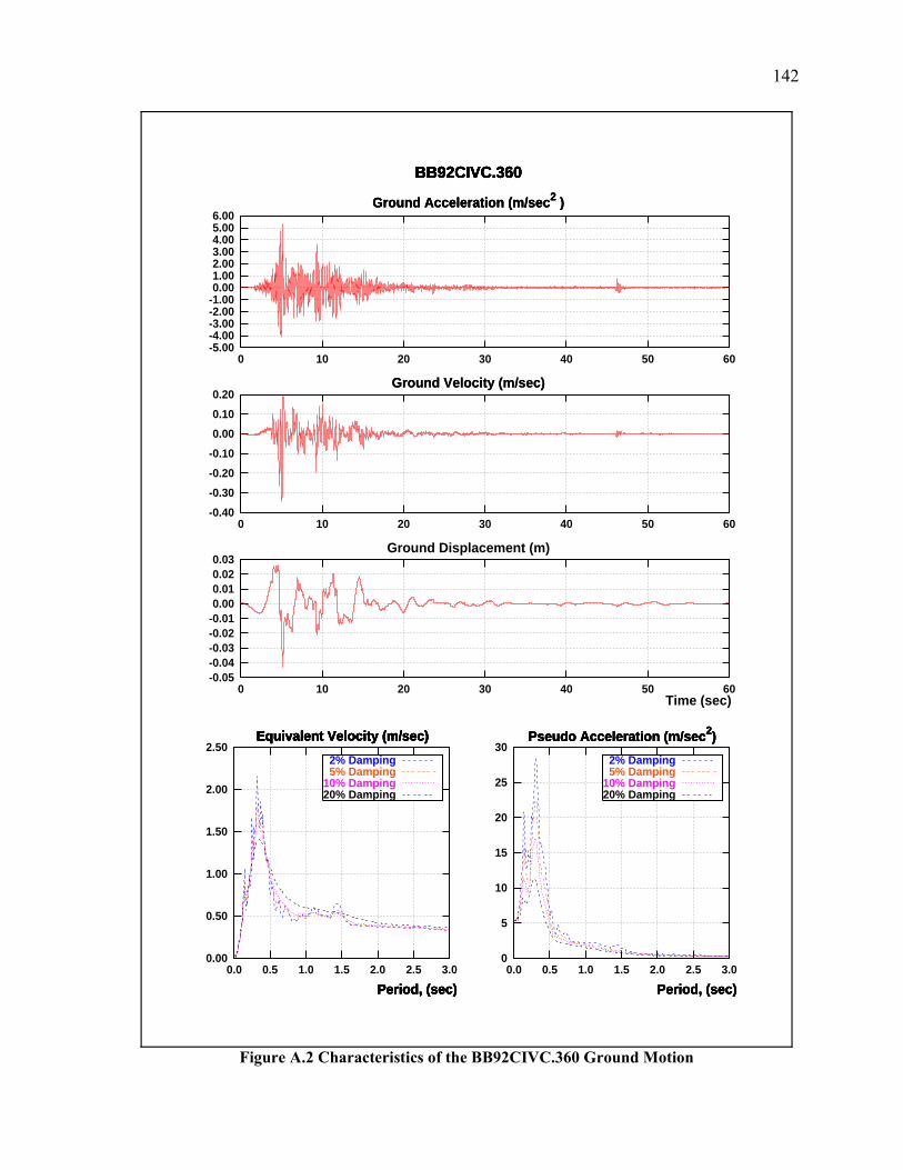
142
Figure A.2 Characteristics of the BB92CIVC.360 Ground Motion
0.00
0.50
1.00
1.50
2.00
2.50
0.0 0.5 1.0 1.5 2.0 2.5 3.0
BB92CIVC.360
Equivalent Velocity (m/sec)
Period, (sec)
2% Damping 5% Damping10% Damping20% Damping
0
5
10
15
20
25
30
0.0 0.5 1.0 1.5 2.0 2.5 3.0
BB92CIVC.360
Equivalent Velocity (m/sec)
Period, (sec)
Pseudo Acceleration (m/sec2)
Period, (sec)
2% Damping 5% Damping10% Damping20% Damping
-5.00-4.00-3.00-2.00-1.000.001.002.003.004.005.006.00
0 10 20 30 40 50 60
BB92CIVC.360
Equivalent Velocity (m/sec)
Period, (sec)
Pseudo Acceleration (m/sec2)
Period, (sec)
Ground Acceleration (m/sec2 )
-0.40
-0.30
-0.20
-0.10
0.00
0.10
0.20
0 10 20 30 40 50 60
BB92CIVC.360
Equivalent Velocity (m/sec)
Period, (sec)
Pseudo Acceleration (m/sec2)
Period, (sec)
Ground Acceleration (m/sec2 )
Ground Velocity (m/sec)
-0.05-0.04-0.03-0.02-0.010.000.010.020.03
0 10 20 30 40 50 60
BB92CIVC.360
Equivalent Velocity (m/sec)
Period, (sec)
Pseudo Acceleration (m/sec2)
Period, (sec)
Ground Acceleration (m/sec2 )
Ground Velocity (m/sec)
Ground Displacement (m)
Time (sec)
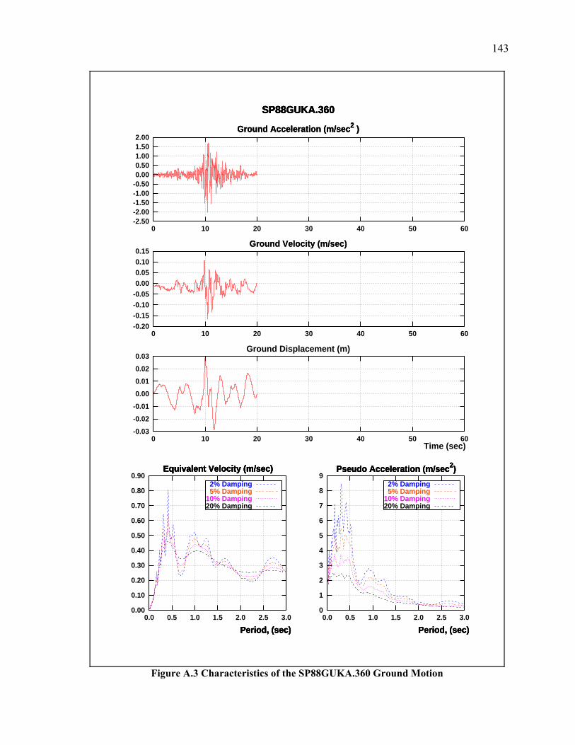
143
Figure A.3 Characteristics of the SP88GUKA.360 Ground Motion
0.00
0.10
0.20
0.30
0.40
0.50
0.60
0.70
0.80
0.90
0.0 0.5 1.0 1.5 2.0 2.5 3.0
SP88GUKA.360
Equivalent Velocity (m/sec)
Period, (sec)
2% Damping 5% Damping10% Damping20% Damping
0
1
2
3
4
5
6
7
8
9
0.0 0.5 1.0 1.5 2.0 2.5 3.0
SP88GUKA.360
Equivalent Velocity (m/sec)
Period, (sec)
Pseudo Acceleration (m/sec2)
Period, (sec)
2% Damping 5% Damping10% Damping20% Damping
-2.50-2.00-1.50-1.00-0.500.000.501.001.502.00
0 10 20 30 40 50 60
SP88GUKA.360
Equivalent Velocity (m/sec)
Period, (sec)
Pseudo Acceleration (m/sec2)
Period, (sec)
Ground Acceleration (m/sec2 )
-0.20-0.15-0.10-0.050.000.050.100.15
0 10 20 30 40 50 60
SP88GUKA.360
Equivalent Velocity (m/sec)
Period, (sec)
Pseudo Acceleration (m/sec2)
Period, (sec)
Ground Acceleration (m/sec2 )
Ground Velocity (m/sec)
-0.03
-0.02
-0.01
0.00
0.01
0.02
0.03
0 10 20 30 40 50 60
SP88GUKA.360
Equivalent Velocity (m/sec)
Period, (sec)
Pseudo Acceleration (m/sec2)
Period, (sec)
Ground Acceleration (m/sec2 )
Ground Velocity (m/sec)
Ground Displacement (m)
Time (sec)

144
Figure A.4 Characteristics of the LP89CORR.090 Ground Motion
0.00
0.50
1.00
1.50
2.00
2.50
3.00
3.50
4.00
0.0 0.5 1.0 1.5 2.0 2.5 3.0
LP89CORR.090
Equivalent Velocity (m/sec)
Period, (sec)
2% Damping 5% Damping10% Damping20% Damping
0
5
10
15
20
25
0.0 0.5 1.0 1.5 2.0 2.5 3.0
LP89CORR.090
Equivalent Velocity (m/sec)
Period, (sec)
Pseudo Acceleration (m/sec2)
Period, (sec)
2% Damping 5% Damping10% Damping20% Damping
-4.00-3.00-2.00-1.000.001.002.003.004.005.00
0 10 20 30 40 50 60
LP89CORR.090
Equivalent Velocity (m/sec)
Period, (sec)
Pseudo Acceleration (m/sec2)
Period, (sec)
Ground Acceleration (m/sec2 )
-0.50-0.40-0.30-0.20-0.100.000.100.200.300.40
0 10 20 30 40 50 60
LP89CORR.090
Equivalent Velocity (m/sec)
Period, (sec)
Pseudo Acceleration (m/sec2)
Period, (sec)
Ground Acceleration (m/sec2 )
Ground Velocity (m/sec)
-0.15
-0.10
-0.05
0.00
0.05
0.10
0.15
0 10 20 30 40 50 60
LP89CORR.090
Equivalent Velocity (m/sec)
Period, (sec)
Pseudo Acceleration (m/sec2)
Period, (sec)
Ground Acceleration (m/sec2 )
Ground Velocity (m/sec)
Ground Displacement (m)
Time (sec)

145
Figure A.5 Characteristics of the NR94CENT.360 Ground Motion
0.00
0.20
0.40
0.60
0.80
1.00
1.20
1.40
1.60
0.0 0.5 1.0 1.5 2.0 2.5 3.0
NR94CENT.360
Equivalent Velocity (m/sec)
Period, (sec)
2% Damping 5% Damping10% Damping20% Damping
0
1
2
3
4
5
6
7
8
9
10
0.0 0.5 1.0 1.5 2.0 2.5 3.0
NR94CENT.360
Equivalent Velocity (m/sec)
Period, (sec)
Pseudo Acceleration (m/sec2)
Period, (sec)
2% Damping 5% Damping10% Damping20% Damping
-2.00-1.50-1.00-0.500.000.501.001.502.002.50
0 10 20 30 40 50 60
NR94CENT.360
Equivalent Velocity (m/sec)
Period, (sec)
Pseudo Acceleration (m/sec2)
Period, (sec)
Ground Acceleration (m/sec2 )
-0.30-0.25-0.20-0.15-0.10-0.050.000.050.100.150.200.25
0 10 20 30 40 50 60
NR94CENT.360
Equivalent Velocity (m/sec)
Period, (sec)
Pseudo Acceleration (m/sec2)
Period, (sec)
Ground Acceleration (m/sec2 )
Ground Velocity (m/sec)
-0.04-0.03-0.02-0.010.000.010.020.030.040.050.060.07
0 10 20 30 40 50 60
NR94CENT.360
Equivalent Velocity (m/sec)
Period, (sec)
Pseudo Acceleration (m/sec2)
Period, (sec)
Ground Acceleration (m/sec2 )
Ground Velocity (m/sec)
Ground Displacement (m)
Time (sec)

146
Figure A.6 Characteristics of the CH85LLEO.010 Ground Motion
0.00
0.50
1.00
1.50
2.00
2.50
3.00
3.50
4.00
4.50
0.0 0.5 1.0 1.5 2.0 2.5 3.0
CH85LLEO.010
Equivalent Velocity (m/sec)
Period, (sec)
2% Damping 5% Damping10% Damping20% Damping
0
5
10
15
20
25
30
35
40
0.0 0.5 1.0 1.5 2.0 2.5 3.0
CH85LLEO.010
Equivalent Velocity (m/sec)
Period, (sec)
Pseudo Acceleration (m/sec2)
Period, (sec)
2% Damping 5% Damping10% Damping20% Damping
-8.00-6.00-4.00-2.000.002.004.006.008.00
0 10 20 30 40 50 60
CH85LLEO.010
Equivalent Velocity (m/sec)
Period, (sec)
Pseudo Acceleration (m/sec2)
Period, (sec)
Ground Acceleration (m/sec2 )
-0.50-0.40-0.30-0.20-0.100.000.100.200.300.40
0 10 20 30 40 50 60
CH85LLEO.010
Equivalent Velocity (m/sec)
Period, (sec)
Pseudo Acceleration (m/sec2)
Period, (sec)
Ground Acceleration (m/sec2 )
Ground Velocity (m/sec)
-0.15
-0.10
-0.05
0.00
0.05
0.10
0.15
0 10 20 30 40 50 60
CH85LLEO.010
Equivalent Velocity (m/sec)
Period, (sec)
Pseudo Acceleration (m/sec2)
Period, (sec)
Ground Acceleration (m/sec2 )
Ground Velocity (m/sec)
Ground Displacement (m)
Time (sec)

147
Figure A.7 Characteristics of the CH85VALP.070 Ground Motion
0.00
0.20
0.40
0.60
0.80
1.00
1.20
0.0 0.5 1.0 1.5 2.0 2.5 3.0
CH85VALP.070
Equivalent Velocity (m/sec)
Period, (sec)
2% Damping 5% Damping10% Damping20% Damping
0
1
2
3
4
5
6
7
8
9
10
0.0 0.5 1.0 1.5 2.0 2.5 3.0
CH85VALP.070
Equivalent Velocity (m/sec)
Period, (sec)
Pseudo Acceleration (m/sec2)
Period, (sec)
2% Damping 5% Damping10% Damping20% Damping
-2.00-1.50-1.00-0.500.000.501.001.502.00
0 10 20 30 40 50 60
CH85VALP.070
Equivalent Velocity (m/sec)
Period, (sec)
Pseudo Acceleration (m/sec2)
Period, (sec)
Ground Acceleration (m/sec2 )
-0.15
-0.10
-0.05
0.00
0.05
0.10
0.15
0 10 20 30 40 50 60
CH85VALP.070
Equivalent Velocity (m/sec)
Period, (sec)
Pseudo Acceleration (m/sec2)
Period, (sec)
Ground Acceleration (m/sec2 )
Ground Velocity (m/sec)
-0.03-0.02-0.010.000.010.020.030.04
0 10 20 30 40 50 60
CH85VALP.070
Equivalent Velocity (m/sec)
Period, (sec)
Pseudo Acceleration (m/sec2)
Period, (sec)
Ground Acceleration (m/sec2 )
Ground Velocity (m/sec)
Ground Displacement (m)
Time (sec)
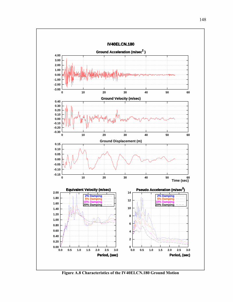
148
Figure A.8 Characteristics of the IV40ELCN.180 Ground Motion
0.00
0.20
0.40
0.60
0.80
1.00
1.20
1.40
1.60
1.80
2.00
0.0 0.5 1.0 1.5 2.0 2.5 3.0
IV40ELCN.180
Equivalent Velocity (m/sec)
Period, (sec)
2% Damping 5% Damping10% Damping20% Damping
0
2
4
6
8
10
12
14
0.0 0.5 1.0 1.5 2.0 2.5 3.0
IV40ELCN.180
Equivalent Velocity (m/sec)
Period, (sec)
Pseudo Acceleration (m/sec2)
Period, (sec)
2% Damping 5% Damping10% Damping20% Damping
-3.00
-2.00
-1.00
0.00
1.00
2.00
3.00
4.00
0 10 20 30 40 50 60
IV40ELCN.180
Equivalent Velocity (m/sec)
Period, (sec)
Pseudo Acceleration (m/sec2)
Period, (sec)
Ground Acceleration (m/sec2 )
-0.30-0.20-0.100.000.100.200.300.40
0 10 20 30 40 50 60
IV40ELCN.180
Equivalent Velocity (m/sec)
Period, (sec)
Pseudo Acceleration (m/sec2)
Period, (sec)
Ground Acceleration (m/sec2 )
Ground Velocity (m/sec)
-0.15
-0.10
-0.05
0.00
0.05
0.10
0.15
0 10 20 30 40 50 60
IV40ELCN.180
Equivalent Velocity (m/sec)
Period, (sec)
Pseudo Acceleration (m/sec2)
Period, (sec)
Ground Acceleration (m/sec2 )
Ground Velocity (m/sec)
Ground Displacement (m)
Time (sec)

149
Figure A.9 Characteristics of the LN92JOSH.360 Ground Motion
0.00
0.50
1.00
1.50
2.00
2.50
0.0 0.5 1.0 1.5 2.0 2.5 3.0
LN92JOSH.360
Equivalent Velocity (m/sec)
Period, (sec)
2% Damping 5% Damping10% Damping20% Damping
0
2
4
6
8
10
12
0.0 0.5 1.0 1.5 2.0 2.5 3.0
LN92JOSH.360
Equivalent Velocity (m/sec)
Period, (sec)
Pseudo Acceleration (m/sec2)
Period, (sec)
2% Damping 5% Damping10% Damping20% Damping
-2.00-1.50-1.00-0.500.000.501.001.502.002.503.00
0 10 20 30 40 50 60
LN92JOSH.360
Equivalent Velocity (m/sec)
Period, (sec)
Pseudo Acceleration (m/sec2)
Period, (sec)
Ground Acceleration (m/sec2 )
-0.30
-0.20
-0.10
0.00
0.10
0.20
0.30
0 10 20 30 40 50 60
LN92JOSH.360
Equivalent Velocity (m/sec)
Period, (sec)
Pseudo Acceleration (m/sec2)
Period, (sec)
Ground Acceleration (m/sec2 )
Ground Velocity (m/sec)
-0.08-0.06-0.04-0.020.000.020.040.060.08
0 10 20 30 40 50 60
LN92JOSH.360
Equivalent Velocity (m/sec)
Period, (sec)
Pseudo Acceleration (m/sec2)
Period, (sec)
Ground Acceleration (m/sec2 )
Ground Velocity (m/sec)
Ground Displacement (m)
Time (sec)
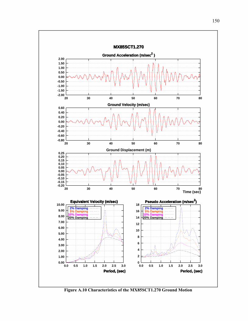
150
Figure A.10 Characteristics of the MX85SCT1.270 Ground Motion
0.00
1.00
2.00
3.00
4.00
5.00
6.00
7.00
8.00
9.00
10.00
0.0 0.5 1.0 1.5 2.0 2.5 3.0
MX85SCT1.270
Equivalent Velocity (m/sec)
Period, (sec)
2% Damping 5% Damping10% Damping20% Damping
0
2
4
6
8
10
12
14
16
18
0.0 0.5 1.0 1.5 2.0 2.5 3.0
MX85SCT1.270
Equivalent Velocity (m/sec)
Period, (sec)
Pseudo Acceleration (m/sec2)
Period, (sec)
2% Damping 5% Damping10% Damping20% Damping
-2.00-1.50-1.00-0.500.000.501.001.502.00
20 30 40 50 60 70 80
MX85SCT1.270
Equivalent Velocity (m/sec)
Period, (sec)
Pseudo Acceleration (m/sec2)
Period, (sec)
Ground Acceleration (m/sec2 )
-0.80-0.60-0.40-0.200.000.200.400.60
20 30 40 50 60 70 80
MX85SCT1.270
Equivalent Velocity (m/sec)
Period, (sec)
Pseudo Acceleration (m/sec2)
Period, (sec)
Ground Acceleration (m/sec2 )
Ground Velocity (m/sec)
-0.20-0.15-0.10-0.050.000.050.100.150.200.25
20 30 40 50 60 70 80
MX85SCT1.270
Equivalent Velocity (m/sec)
Period, (sec)
Pseudo Acceleration (m/sec2)
Period, (sec)
Ground Acceleration (m/sec2 )
Ground Velocity (m/sec)
Ground Displacement (m)
Time (sec)

151
Figure A.11 Characteristics of the LN92LUCN.250 Ground Motion
0.00
0.20
0.40
0.60
0.80
1.00
1.20
1.40
1.60
1.80
0.0 0.5 1.0 1.5 2.0 2.5 3.0
LN92LUCN.250
Equivalent Velocity (m/sec)
Period, (sec)
2% Damping 5% Damping10% Damping20% Damping
0
5
10
15
20
25
30
35
0.0 0.5 1.0 1.5 2.0 2.5 3.0
LN92LUCN.250
Equivalent Velocity (m/sec)
Period, (sec)
Pseudo Acceleration (m/sec2)
Period, (sec)
2% Damping 5% Damping10% Damping20% Damping
-8.00-6.00-4.00-2.000.002.004.006.008.00
0 10 20 30 40 50 60
LN92LUCN.250
Equivalent Velocity (m/sec)
Period, (sec)
Pseudo Acceleration (m/sec2)
Period, (sec)
Ground Acceleration (m/sec2 )
-1.40-1.20-1.00-0.80-0.60-0.40-0.200.000.200.400.600.80
0 10 20 30 40 50 60
LN92LUCN.250
Equivalent Velocity (m/sec)
Period, (sec)
Pseudo Acceleration (m/sec2)
Period, (sec)
Ground Acceleration (m/sec2 )
Ground Velocity (m/sec)
-1.60-1.40-1.20-1.00-0.80-0.60-0.40-0.200.000.200.40
0 10 20 30 40 50 60
LN92LUCN.250
Equivalent Velocity (m/sec)
Period, (sec)
Pseudo Acceleration (m/sec2)
Period, (sec)
Ground Acceleration (m/sec2 )
Ground Velocity (m/sec)
Ground Displacement (m)
Time (sec)

152
Figure A.12 Characteristics of the LP89SARA.360 Ground Motion
0.00
0.20
0.40
0.60
0.80
1.00
1.20
1.40
1.60
1.80
2.00
0.0 0.5 1.0 1.5 2.0 2.5 3.0
LP89SARA.360
Equivalent Velocity (m/sec)
Period, (sec)
2% Damping 5% Damping10% Damping20% Damping
0
2
4
6
8
10
12
14
16
18
20
0.0 0.5 1.0 1.5 2.0 2.5 3.0
LP89SARA.360
Equivalent Velocity (m/sec)
Period, (sec)
Pseudo Acceleration (m/sec2)
Period, (sec)
2% Damping 5% Damping10% Damping20% Damping
-5.00-4.00-3.00-2.00-1.000.001.002.003.00
0 10 20 30 40 50 60
LP89SARA.360
Equivalent Velocity (m/sec)
Period, (sec)
Pseudo Acceleration (m/sec2)
Period, (sec)
Ground Acceleration (m/sec2 )
-0.50-0.40-0.30-0.20-0.100.000.100.200.30
0 10 20 30 40 50 60
LP89SARA.360
Equivalent Velocity (m/sec)
Period, (sec)
Pseudo Acceleration (m/sec2)
Period, (sec)
Ground Acceleration (m/sec2 )
Ground Velocity (m/sec)
-0.10
-0.05
0.00
0.05
0.10
0.15
0.20
0 10 20 30 40 50 60
LP89SARA.360
Equivalent Velocity (m/sec)
Period, (sec)
Pseudo Acceleration (m/sec2)
Period, (sec)
Ground Acceleration (m/sec2 )
Ground Velocity (m/sec)
Ground Displacement (m)
Time (sec)
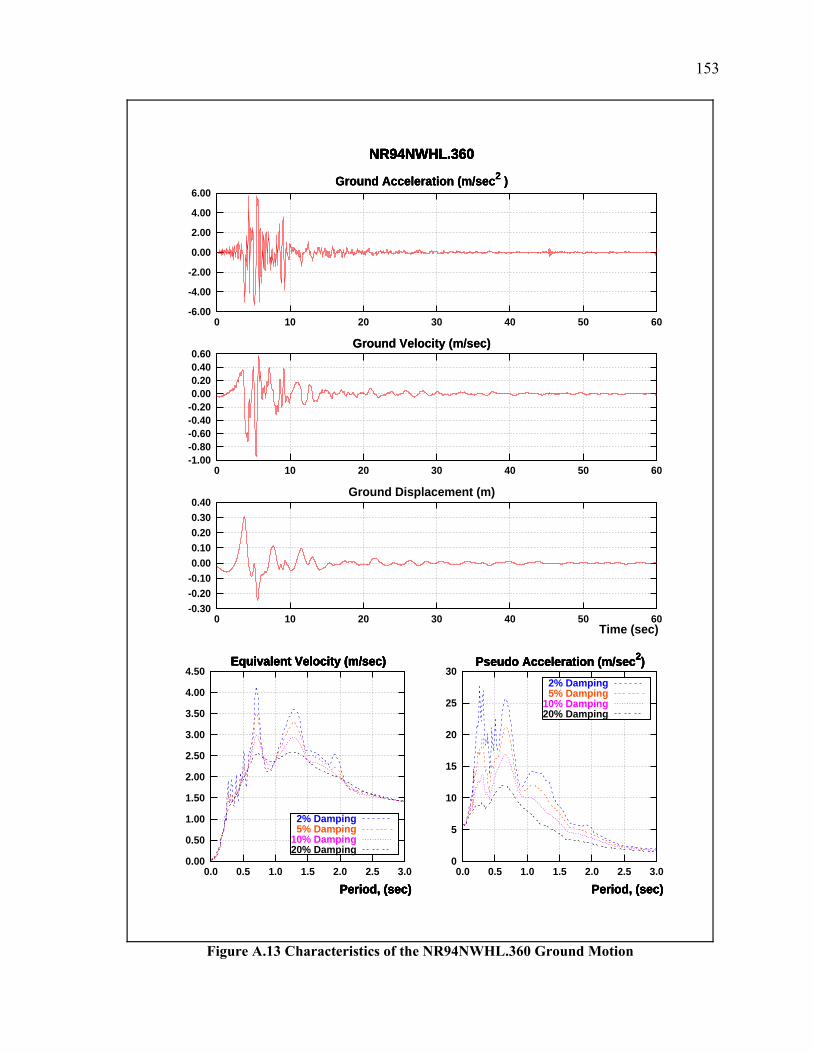
153
Figure A.13 Characteristics of the NR94NWHL.360 Ground Motion
0.00
0.50
1.00
1.50
2.00
2.50
3.00
3.50
4.00
4.50
0.0 0.5 1.0 1.5 2.0 2.5 3.0
NR94NWHL.360
Equivalent Velocity (m/sec)
Period, (sec)
2% Damping 5% Damping10% Damping20% Damping
0
5
10
15
20
25
30
0.0 0.5 1.0 1.5 2.0 2.5 3.0
NR94NWHL.360
Equivalent Velocity (m/sec)
Period, (sec)
Pseudo Acceleration (m/sec2)
Period, (sec)
2% Damping 5% Damping10% Damping20% Damping
-6.00
-4.00
-2.00
0.00
2.00
4.00
6.00
0 10 20 30 40 50 60
NR94NWHL.360
Equivalent Velocity (m/sec)
Period, (sec)
Pseudo Acceleration (m/sec2)
Period, (sec)
Ground Acceleration (m/sec2 )
-1.00-0.80-0.60-0.40-0.200.000.200.400.60
0 10 20 30 40 50 60
NR94NWHL.360
Equivalent Velocity (m/sec)
Period, (sec)
Pseudo Acceleration (m/sec2)
Period, (sec)
Ground Acceleration (m/sec2 )
Ground Velocity (m/sec)
-0.30-0.20-0.100.000.100.200.300.40
0 10 20 30 40 50 60
NR94NWHL.360
Equivalent Velocity (m/sec)
Period, (sec)
Pseudo Acceleration (m/sec2)
Period, (sec)
Ground Acceleration (m/sec2 )
Ground Velocity (m/sec)
Ground Displacement (m)
Time (sec)
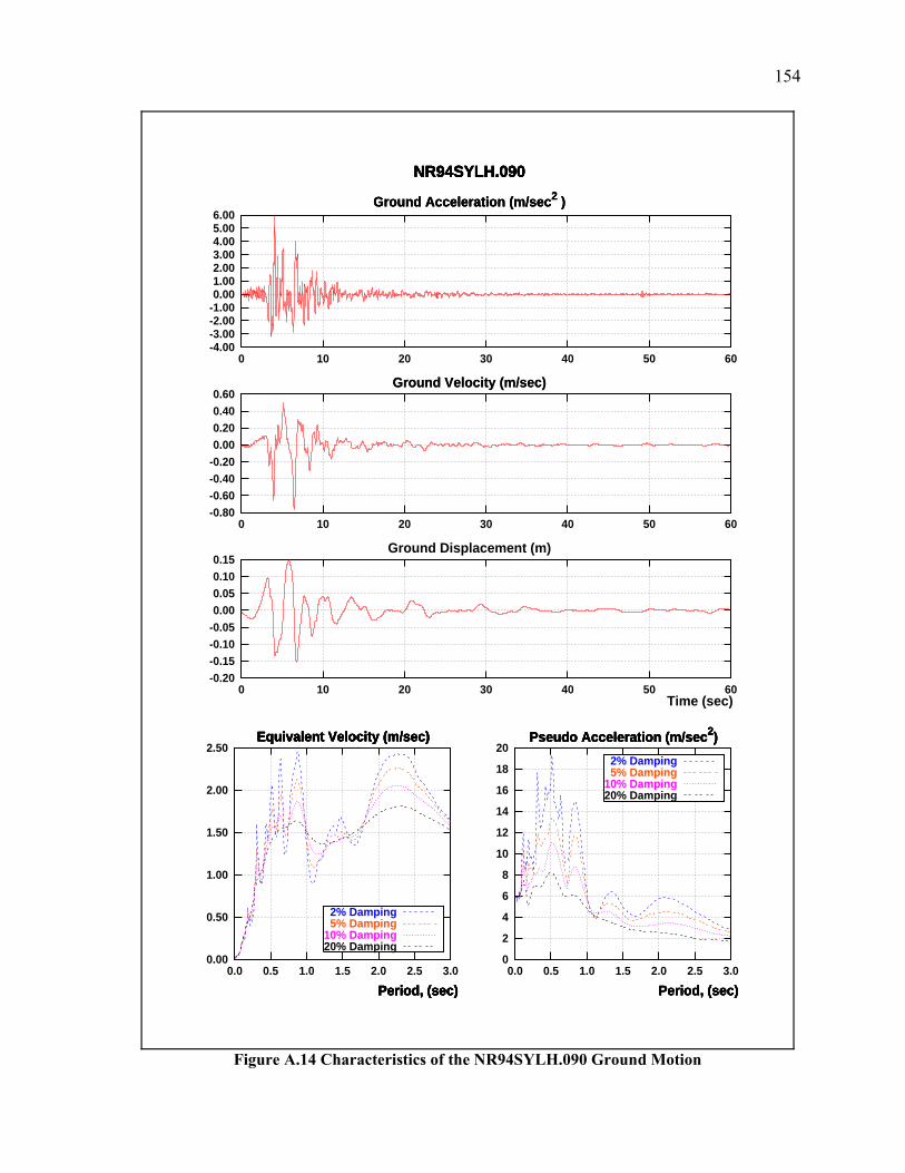
154
Figure A.14 Characteristics of the NR94SYLH.090 Ground Motion
0.00
0.50
1.00
1.50
2.00
2.50
0.0 0.5 1.0 1.5 2.0 2.5 3.0
NR94SYLH.090
Equivalent Velocity (m/sec)
Period, (sec)
2% Damping 5% Damping10% Damping20% Damping
0
2
4
6
8
10
12
14
16
18
20
0.0 0.5 1.0 1.5 2.0 2.5 3.0
NR94SYLH.090
Equivalent Velocity (m/sec)
Period, (sec)
Pseudo Acceleration (m/sec2)
Period, (sec)
2% Damping 5% Damping10% Damping20% Damping
-4.00-3.00-2.00-1.000.001.002.003.004.005.006.00
0 10 20 30 40 50 60
NR94SYLH.090
Equivalent Velocity (m/sec)
Period, (sec)
Pseudo Acceleration (m/sec2)
Period, (sec)
Ground Acceleration (m/sec2 )
-0.80-0.60-0.40-0.200.000.200.400.60
0 10 20 30 40 50 60
NR94SYLH.090
Equivalent Velocity (m/sec)
Period, (sec)
Pseudo Acceleration (m/sec2)
Period, (sec)
Ground Acceleration (m/sec2 )
Ground Velocity (m/sec)
-0.20-0.15-0.10-0.050.000.050.100.15
0 10 20 30 40 50 60
NR94SYLH.090
Equivalent Velocity (m/sec)
Period, (sec)
Pseudo Acceleration (m/sec2)
Period, (sec)
Ground Acceleration (m/sec2 )
Ground Velocity (m/sec)
Ground Displacement (m)
Time (sec)

155
Figure A.15 Characteristics of the KO95TTRI.360 Ground Motion
0.00
1.00
2.00
3.00
4.00
5.00
6.00
7.00
8.00
0.0 0.5 1.0 1.5 2.0 2.5 3.0
KO95TTRI.360
Equivalent Velocity (m/sec)
Period, (sec)
2% Damping 5% Damping10% Damping20% Damping
0
5
10
15
20
25
30
0.0 0.5 1.0 1.5 2.0 2.5 3.0
KO95TTRI.360
Equivalent Velocity (m/sec)
Period, (sec)
Pseudo Acceleration (m/sec2)
Period, (sec)
2% Damping 5% Damping10% Damping20% Damping
-6.00
-4.00
-2.00
0.00
2.00
4.00
6.00
8.00
0 10 20 30 40 50 60
KO95TTRI.360
Equivalent Velocity (m/sec)
Period, (sec)
Pseudo Acceleration (m/sec2)
Period, (sec)
Ground Acceleration (m/sec2 )
-1.50
-1.00
-0.50
0.00
0.50
1.00
1.50
0 10 20 30 40 50 60
KO95TTRI.360
Equivalent Velocity (m/sec)
Period, (sec)
Pseudo Acceleration (m/sec2)
Period, (sec)
Ground Acceleration (m/sec2 )
Ground Velocity (m/sec)
-0.40-0.30-0.20-0.100.000.100.200.30
0 10 20 30 40 50 60
KO95TTRI.360
Equivalent Velocity (m/sec)
Period, (sec)
Pseudo Acceleration (m/sec2)
Period, (sec)
Ground Acceleration (m/sec2 )
Ground Velocity (m/sec)
Ground Displacement (m)
Time (sec)

156
APPENDIX B
C++ PROGRAM FOR DISPLACEMENT COEFFICIENT METHOD ESTIMATES
This appendix presents the listing of a computer program implementing the
Displacement Coefficient Method. The program is written using the programing language
C++ and is called DCM. No units are implicit in the program, therefore the input data must
be provided in consistent units.
The syntax to use the program is as follows:
DCM record_file_name To effective_period damping W VyMDOF C0 C2 C3
where:
record_file_name is the name of a file containing the acceleration ground motion,To is the characteristic period of the ground motion,effective_period is the period assumed for the equivalent SDOF system,W is the total weight of the multistory system,Vy
MDOF is the strength of the multistory system, andC0, C2, C3 are as defined in the Displacement Coefficient Method.
The value of C1, the modification factor to relate expected maximum inelastic
displacement to displacement calculated for linear elastic response, is calculated by the
program.
For all the results of the Displacement Coefficient Method shown along this work, the
valued of C2 and C3 were assumed as one (1).
All the numerical parameters used to run the DCM program are floating points
numbers.
The structure of the record containing the acceleration ground motion is as follows:
1st line; void line. May be used to identify the ground motion.
2nd line; one floating point number. Used to scale the ground motion accelerations.
3rd line; integer number. Number of data points in the acceleration record.
The rest of the file consists of two floating point numbers per line. The first number is
the time and the second number is the acceleration.
Following is the list of the DCM program.
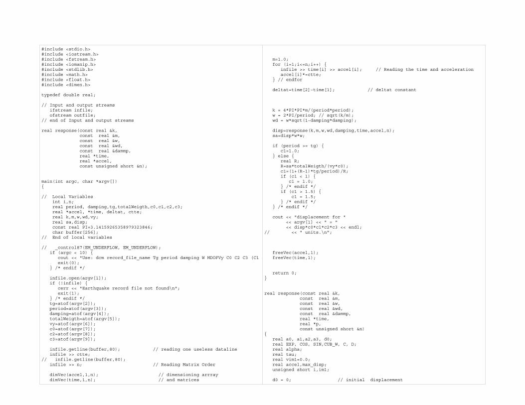
#include <stdio.h>#include <iostream.h>#include <fstream.h>#include <iomanip.h>#include <stdlib.h>#include <math.h>#include <float.h>#include <dimen.h>
typedef double real;
// Input and output streamsifstream infile;ofstream outfile;
// end of Input and output streams
real response(const real &k,const real &m,const real &w,const real &wd,const real &dammp,real *time,real *accel,const unsigned short &n);
main(int argc, char *argv[]){
// Local Variablesint i,n;real period, damping,tg,totalWeigth,c0,c1,c2,c3;real *accel, *time, deltat, ctte;real k,m,w,wd,vy;real sa,disp;const real PI=3.14159265358979323846;char buffer[256];
// End of local variables
// _control87(EM_UNDERFLOW, EM_UNDERFLOW);if (argc < 10) {
cout << "Use: dcm record_file_name Tg period damping W MDOFVy C0 C2 C3 (C1 iexit(0);
} /* endif */
infile.open(argv[1]);if (!infile) {
cerr << "Earthquake record file not found\n";exit(1);
} /* endif */tg=atof(argv[2]);period=atof(argv[3]);damping=atof(argv[4]);totalWeigth=atof(argv[5]);vy=atof(argv[6]);c0=atof(argv[7]);c2=atof(argv[8]);c3=atof(argv[9]);
infile.getline(buffer,80); // reading one useless datalineinfile >> ctte;
// infile.getline(buffer,80);infile >> n; // Reading Matrix Order
dimVec(accel,1,n); // dimensioning arrraydimVec(time,1,n); // and matrices
m=1.0; for (i=1;i<=n;i++) {
infile >> time[i] >> accel[i]; // Reading the time and accelerationaccel[i]*=ctte;
} // endfor
deltat=time[2]−time[1]; // deltat constant
k = 4*PI*PI*m/(period*period);w = 2*PI/period; // sqrt(k/m);wd = w*sqrt(1−damping*damping);
disp=response(k,m,w,wd,damping,time,accel,n);sa=disp*w*w;
if (period >= tg) {c1=1.0;
} else {real R;R=sa*totalWeigth/(vy*c0);c1=(1+(R−1)*tg/period)/R;if (c1 < 1) {
c1 = 1.0;} /* endif */if (c1 > 1.5) {
c1 = 1.5;} /* endif */
} /* endif */
cout << "displacement for " << argv[1] << " = " << disp*c0*c1*c2*c3 << endl;
// << " units.\n";
freeVec(accel,1);freeVec(time,1);
return 0;}
real response(const real &k,const real &m,const real &w,const real &wd,const real &dammp,real *time,real *p,const unsigned short &n)
{real a0, a1,a2,a3, d0;real EXP, COS, SIN,CUB_W, C, D;real alpha;real tau;real vim1=0.0;real accel,max_disp;unsigned short i,im1;
d0 = 0; // initial displacement
max_disp = 0.0; tau = time[2] − time[1];EXP = exp(−dammp*w*tau);COS = cos(wd*tau);SIN = sin(wd*tau);CUB_W = w*w*w;
for (i=2,im1=1;i<=n+1;i++,im1++) {alpha = (p[i]−p[im1])/tau;a0 = p[im1]/k −2*dammp*alpha/(m*CUB_W);a1 = alpha/k;a2 = d0 − a0;a3 = (vim1 + dammp*w*a2 − a1)/wd;C = (wd*a3−dammp*w*a2);D = (a2*wd+dammp*w*a3);
d0 = a0 + a1*tau + a2*EXP*COS + a3*EXP*SIN;vim1 = a1 + C*EXP*COS − D*EXP*SIN;
if (fabs(d0) > max_disp) {max_disp = fabs(d0);
} /* endif */} /* endfor */return (max_disp);
}
++++++++++++++++++++++++++++ dimen.h ++++++++++++++++++++++++++
#ifndef DIMEN_H#define DIMEN_H#include<iostream.h>#include<stdlib.h>
template <class T, class entero>void dimVec(T *(&v),
const int offset,const entero size)
{v = new T [size];if (!v) {cout << "(V)No hay suficiente memoria para analizar este problema" << endl ;exit (1);
}v −= offset;
}
template <class T, class entero>void dimMat(T **(&m),
const int nrl,const entero nrow,const int ncl,const entero ncol)
{unsigned long i, nrh;
nrh=nrow+nrl−1;
m = (T **) new T* [nrow];if (!m) {cout << "(M1)No hay suficiente memoria para analizar este problema" << endl
exit (1);}m −= nrl;m[nrl]= new T [nrow*ncol];if (!m[nrl]) {cout << "(M2)No hay suficiente memoria para analizar este problema" << endl exit (1);
}m[nrl]−= ncl;for (i=nrl+1;i<=nrh;i++)
m[i] = m[i−1]+ncol;/* endfor */
}
template <class T>void freeVec(T *(&v),
const int offsets){
delete (v+offsets);}
template <class T>void freeMat(T **(&m),
const int nrl,const int ncl)
{m[nrl] += ncl;delete m[nrl];m += nrl;delete[] m;
}#endif // End of dinen.h
++++++++++++++++++++++++++++ dimen.h ++++++++++++++++++++++++++

159
APPENDIX C
C++ PROGRAM FOR CAPACITY SPECTRUM METHOD ESTIMATES
This appendix presents the listing of a computer program implementing the Capacity
Spectrum. The program is written using the programing language C++ and is referenced as
CSM. No units are implicit in the program, therefore the input data must be provided in
consistent units.
The syntax to use the program is as follows:
CSM record_file_name VySDOF uy
SDOF post-yield_stiffness(%) PF1 To
where:
record_file_name is the name of a file containing the acceleration groundmotion,
VySDOF is the strength of the equivalent SDOF,
uySDOF is the yield displacement of the equivalent SDOF,
post-yield_stiffness(%): is the post-yield stiffness expressed as a percentage ofinitial stiffness,
PF1 is the participation factor, andTo is the characteristic period of the ground motion.
All the numerical parameters used to run the CSM program are floating point
numbers.
The structure of the record containing the acceleration ground motion is as follows:
1st line; void line. May be used to identify the ground motion.
2nd line; one floating point number. Used to scale the ground motion accelerations.
3rd line; integer number. Number of data points in the acceleration record.
The rest of the file consists of two floating point numbers per line. The first number is
the time and the second number is the acceleration.
Following is the list of the CSM program.

#include <stdio.h>#include <iostream.h>#include <fstream.h>#include <iomanip.h>#include <stdlib.h>#include <math.h>#include <float.h>#include <dimen.h>
typedef double real;
// Input and output streamsifstream infile;ofstream outfile;
// end of Input and output streams
real response(const real &k,const real &m,const real &w,const real &wd,const real &dammp,real *time,real *accel,const unsigned short &n);
main(int argc, char *argv[]){
// Local Variablesconst int nmax = 100;const real PI=3.14159265358979323846;char buffer[256];int i, n, count=0 ;real dy,fy,pys,pf1, tg;real ca, cv;real k, m, period, w, wd;real dpi,fpi,deltat,ctte,damping,b0,beff,k_factor;real sra, srv,Ts;real olddpi, temp;real *time, *accel;
// End of local variables
// _control87(EM_UNDERFLOW, EM_UNDERFLOW);if (argc < 6) {
cout << "Use: csmv2 record_file_name SDOFVy SDOFdy post−yield_stiffnesexit(0);
} /* endif */
infile.open(argv[1]);if (!infile) {
cerr << "Earthquake record file not found\n";exit(1);
} /* endif */fy=atof(argv[2]);dy=atof(argv[3]);k = fy/dy;pys=atof(argv[4])*.01*k;pf1=atof(argv[5]);tg=atof(argv[6]);
infile.getline(buffer,80); // reading one useless datalineinfile >> ctte;
// infile.getline(buffer,80);infile >> n; // Reading Matrix Order
dimVec(accel,1,n); // dimensioning arrraydimVec(time,1,n); // and matrices
for (i=1;i<=n;i++) {infile >> time[i] >> accel[i]; // Reading the time and accelerationaccel[i]*=ctte;if (fabs(accel[i]) > ca) {
ca=fabs(accel[i]);} /* endif */
} // endfor cv= 2.5*ca*tg;
deltat=time[2]−time[1]; // deltat constantm=1.0;damping=beff=.05; // to start withperiod=2*PI*sqrt(m/k);w = 2*PI/period; // sqrt(k/m);wd = w*sqrt(1−damping*damping);dpi=response(k,m,w,wd,damping,time,accel,n);
if (dpi > dy) {// fpi=fy+pys*(dpi−dy);
do {count ++;fpi=fy+pys*(dpi−dy);
b0=2*(fy*dpi−dy*fpi)/(PI*fpi*dpi);
if (b0 <= .1625) { //k_factor=1.0; //
} else if (b0 >= .45) { // This is consistent withk_factor=7/9; // Fig. 8.15 ATC−40
} else { // type A structuresk_factor=1.0 − 8/10.35*(b0 −.1625); //
} /* endif */ //
beff=b0*k_factor+0.05; // if (beff > 0.40) { //
beff = 0.4; // This is consistent wit} else if (beff < 0.05){ // Fig. 8.16 ATC−40
beff = 0.05; // type A structures } /* endif */ //
//
sra=(3.21−0.68*log(beff*100))/2.12; // Eq. 8.9srv=(2.31−0.41*log(beff*100))/1.65; // Eq. 8.10
if (sra < 0.33) {sra = 0.33;
} /* endif */if (srv < 0.50) {
srv = 0.50;} /* endif */
Ts=srv*cv/(2.5*sra*ca);
k=fpi/dpi;period=2*PI*sqrt(m/k);w = sqrt(k/m); // sqrt(k/m);wd = w*sqrt(1−damping*damping);olddpi=dpi;dpi=response(k,m,w,wd,damping,time,accel,n); if (period > Ts) {
dpi=dpi*srv;} else {


![Seismic performance evaluation of Egyptian code-designed ... · parametric and comparative studies [1–7]. These studies ... the shaking table testing of multistory reinforced concrete](https://static.fdocuments.in/doc/165x107/5fcb8346d98df67a9a6c84fa/seismic-performance-evaluation-of-egyptian-code-designed-parametric-and-comparative.jpg)


