Segmentation of Subcortical structures in T1 weighted MRI ... · cles are signs of AD progression...

Segmentation of Subcorticalstructures in T1 weighted MRI as a

component of a Brain AtrophyComputation Pipeline

Master ThesisCecilie Benedicte Anker

Biomediq A/S&

Technical University of Denmark, DTU

Supervised by:Prof. Mads Nielsen, KU, Prof. Rasmus Larsen, DTU,

Prof. Knut Conradsen, DTU, & Postdoc Mark Lyksborg, DTU.2014

Technical University of DenmarkDTU ComputeBuilding 303B, DK-2800 Kongens Lyngby, DenmarkPhone +45 45253031, Fax +45 [email protected]

Abstract

Among the top performing automated hippocampal segmentation methods fromstructural Magnetic Resonance Imaging (MRI), are multi-atlas segmentationmethods, which rely on manual annotations.

In this thesis two fundamentally different multi-atlas segmentation methodsare implemented, N-L Patch and BrainFuseLab. In N-L Patch, each voxel issegmented using information from atlases which have been coarsely aligned usingaffine registrations. BrainFuseLab aligns atlases using non-rigid registrations,and is thus comparatively slower. To make a fair comparison, both methods willuse the same atlases from a new Harmonized Hippocampal Protocol (HHP).

Method parameters are optimized in a leave-one-out cross-validation using twodifferent atlas sets. Based on volume overlap with the manual annotations, N-LPatch is chosen to segment a standardized ADNI dataset containing 1.5T MRIsfrom 504 diagnosed subjects (169 cognitively normal (CN), 234 mild cognitiveimpairment (MCI), 101 alzheimer’s disease (AD)) at baseline, month 12 andmonth 24. Hippocampal atrophy calculated as percentage volume change frombaseline to follow-up is estimated. Based on a statistical analysis, the diagnosticgroup separation capabilities of N-L Patch are compared to two state-of-the-artmethods, cross-sectional FreeSurfer and longitudinal FreeSurfer.

Including the HHP annotations in N-L Patch yielded significantly better groupseparation than cross-sectional FreeSurfer in separating AD from CN and ADfrom MCI. This illustrates the longitudinal robustness of segmentations whenannotations from the new hippocampal standard are included in automatedsegmentation methods. Also longitudinal FreeSurfer exploiting baseline andfollow-up simultaneously showed no diagnostic improvement over N-L Patch.

Resume

Multi-atlas segmenteringsmetoder med manuelle annoteringer er blandt de bed-ste automatiske hippocampus segmenteringsmetoder til strukturel MagnetiskResonans (MR) billeder.

I denne afhandling er to fundamentalt forskellige multi-atlas segmenteringsme-toder implementeret, N-L Patch og BrainFuseLab. I N-L Patch er hver voxelsegmenteret ved at bruge information fra atlaser, der er groft rettet ind ved affineregistreringer. BrainFuseLab retter atlaserne ind ved brug af ikke-rigide reg-istreringer og er derfor relativt langsommere beregningsmæssigt. Begge metoderbenytter de samme atlaser fra en ny Harmoniseret Hippocampus Protokol (HHP).

Metodeparametre er optimerede i en leave-one-out krydsvalidering. Baseretpa volumenoverlap med de manuelle annoteringer er N-L Patch valgt til atsegmentere et standardiseret ADNI datasæt der indeholder 1.5T MR billederfra 504 diagnostiserede forsøgspersoner (169 kognitiv normal (CN), 234 mildkognitiv forringelse (MCI), 101 alzheimers sygdom (AD)) ved udgangspunktet,maned 12 og maned 24. Hippocampusatrofi, beregnet som den procentviseforskel fra udgangspunktet til opfølgning, er estimeret. Ud fra en statistiskanalyse, er N-L Patchs diagnostiske separationsevne sammenlignet med to state-of-the-art metoder, cross-sectional FreeSurfer og longitidinal FreeSurfer.

Ved at inkludere HHP annoteringer i N-L Patch fas signifikant bedre adskillelseaf AD fra CN og AD fra MCI end for cross-sectional FreeSurfer. Dette illustr-erer segmenteringsrobusthed over tid nar annoteringer fra den nye hippocampusstandard inkluderes i automatiske segmenteringsmetoder. Ogsa longitudinalFreeSurfer, der bruger information fra udgangspunkt og opfølgning samtidig,viste ingen forbedret diagnostisk separationsevne i forhold til N-L Patch.

iv Resume

Preface

This thesis was prepared at the Department of Applied Mathematics and Com-puter Science (DTU Compute) at the Technical University of Denmark (DTU)in partial fulfillment of the requirements for acquiring the Master of ScienceDegree in Engineering, M.Sc.Eng.The undersigned is a Master student in Medicine & Technology at the Tech-nical University of Denmark and the Faculty of Health Sciences, University ofCopenhagen (KU).The work was carried out at the company Biomediq A/S, Fruebjergvej 3, 2100Copenhagen, Denmark. The thesis was supervised by Professor Rasmus Larsen(DTU), Professor Knut Conradsen (DTU), Postdoc Mark Lyksborg (DTU) andProfessor Mads Nielsen (Biomediq A/S & KU). The work was carried out fromSeptember 2013 to February 2014, corresponding to 30 ECTS credits.

Copenhagen, February 2014

Cecilie Benedicte Anker

Acknowledgements

I would like to thank my DTU supervisors Professor Rasmus Larsen, ProfessorKnut Conradsen and Postdoc Mark Lyksborg for their inputs during the weeklyFriday meetings. A special thanks to Mark Lyksborg for helping me combiningregistrations in SPM.

I thank Professor Mads Nielsen from Biomediq A/S for advise and suggestionsduring supervision meetings and weekly meetings in the Alzheimer’s group atBiomediq A/S. I have very much appreciated working on equal terms with theother employees.

A special thanks to PhD student Akshay Pai and Postdoc Lauge Sørensen fromBiomediq A/S for helping with practicalities of any kind including finding rele-vant literature and to introduce me to the cluster file system.

For helping me to choose appropriate methods to implement, I would like tothank Associate Professor Koen Van Leemput and PhD student Oula Puonti,DTU. Furthermore, I thank Oula Puonti for advise regarding installation ofBrainFuseLab.

Contents

Abstract i

Resume iii

Preface v

Acknowledgements vii

1 Introduction 1

1.1 Clinical background . . . . . . . . . . . . . . . . . . . . . . . . . 3

1.2 Current method . . . . . . . . . . . . . . . . . . . . . . . . . . . . 5

1.3 Project goals . . . . . . . . . . . . . . . . . . . . . . . . . . . . . 8

1.4 Thesis overview . . . . . . . . . . . . . . . . . . . . . . . . . . . . 9

2 State-of-the-art 11

2.1 Method choice . . . . . . . . . . . . . . . . . . . . . . . . . . . . 16

3 Data and Atlases 17

3.1 Data . . . . . . . . . . . . . . . . . . . . . . . . . . . . . . . . . . 17

3.2 Atlases . . . . . . . . . . . . . . . . . . . . . . . . . . . . . . . . . 19

4 Preprocessing 23

4.1 MRI preprocessing . . . . . . . . . . . . . . . . . . . . . . . . . . 23

4.2 Registration and label transformation . . . . . . . . . . . . . . . 27

5 Segmentation methods 37

5.1 Non-Local Patch-based segmentation . . . . . . . . . . . . . . . . 37

5.2 BrainFuseLab . . . . . . . . . . . . . . . . . . . . . . . . . . . . . 42

x CONTENTS

6 Parameter and method selection 476.1 Atlas15 - Leave-one-out cross-validation . . . . . . . . . . . . . . 486.2 Atlas40 - Leave-one-out cross-validation . . . . . . . . . . . . . . 576.3 Evaluation . . . . . . . . . . . . . . . . . . . . . . . . . . . . . . . 65

7 Final results 677.1 Method . . . . . . . . . . . . . . . . . . . . . . . . . . . . . . . . 687.2 Segmentation results . . . . . . . . . . . . . . . . . . . . . . . . . 707.3 Statistical analysis . . . . . . . . . . . . . . . . . . . . . . . . . . 737.4 Discussion . . . . . . . . . . . . . . . . . . . . . . . . . . . . . . . 81

8 Conclusion 858.1 Future Work . . . . . . . . . . . . . . . . . . . . . . . . . . . . . 87

A Atlas Demographics 89

B Statistical Analysis 91B.1 Volume results . . . . . . . . . . . . . . . . . . . . . . . . . . . . 91B.2 Atrophy histograms . . . . . . . . . . . . . . . . . . . . . . . . . 94B.3 Bartlett’s Test . . . . . . . . . . . . . . . . . . . . . . . . . . . . 96B.4 ROC curves . . . . . . . . . . . . . . . . . . . . . . . . . . . . . . 96

C Data CD 99

Chapter 1

Introduction

In the United States, 45% of all people above 85 years suffer from the mostcommon form of dementia, Alzheimer’s disease (AD). The prevalence increaseswith the average lifetime year by year.Payments for AD patients care for 2012 were estimated to be $200 billion in theUnited States, but the amount is expected to increase to $1,1 trillion in 2050(in 2012 dollars) if medication is not improved [20].

AD is pathologically characterized by the presence of intracellular neurofibrillarytangles made of tau protein, extracellular amyloid plaques and decreasing brainvolume (atrophy) due to death of brain cells (neurons). The steadily decreasingnumber of neurons affect a persons behavior, memory and ability to think clearly.At some point, the brain changes impair the ability to carry out basic functionssuch as swallowing and ultimately AD is fatal. At the moment no cure for ADis on the market [20].Figure 1.1 illustrates that deaths caused by AD have continued to rise, whileother major causes of death have decreased in the past years. This clarifies theneed for developing new medication, which can cure AD or significantly decreasethe disease progression rate.

One of the subcortical brain structures showing early pathological atrophy inAD is hippocampus, which is associated with consolidation of information fromshort-term memory to long-term memory and spatial navigation.

2 Introduction

Figure 1.1: Percentage changes in selected Causes of Death (Allages) between 2000 and 2008 [20].

Hippocampal volumetry derived from structural Magnetic Resonance Imaging(MRI) has been endorsed by the new AD diagnostic guidelines as a radiologicalmarker of disease progression [27] and proposed as a part of a new criteria toallow diagnosis of AD to be made earlier than it would be possible on pureclinical grounds [3]. Therefore, it is needed to segment the structure from T1-weighted MRI to analyze shape, volume and texture changes. A delimitation ofhippocampus (blue) from MRI in a coronal, sagittal and transversal view canbe seen in Figure 1.2. As the figure illustrates, a person has two hippocampi,one in each brain hemisphere.

Figure 1.2: Segmentation of hippocampus (blue) from T1-weightedMRI, coronal, sagittal and transversal view.

Manual segmentations of subcortical structures are very time consuming andare subject to errors [4]. To be practicable for studies with many subjects andin clinical applications, automated segmentation is needed [15]. This thesis willconcern automated hippocampal segmentation from T1-weighted MRI.

1.1 Clinical background 3

1.1 Clinical background

In recent years, AD research has emphasized that decline in pathological pro-cesses and clinical functions occur gradually with dementia representing the endstage of many years of accumulation of these pathological changes. The patho-logical changes begin to occur decades before the earliest clinical symptoms [24].The hypothesis is, that the pathological changes begin with abnormal process-ing of amyloid precursor protein (APP). APP leads to excess production orreduced clearance of β-amyloid (Aβ) in the cortex. Some of the Aβ-residues,especially Aβ42, are highly hydrophobic and forms oligomers and fibrils, whichaccumulate as extracellular plaques. Furthermore, the Aβ oligomers lead to acascade characterized by abnormal tau aggregation called neurofibrillary tangles(NFTs) inside the neurons, synaptic dysfunction, cell death, localized atrophyand eventually whole brain atrophy. Whole brain atrophy and enlarged ventri-cles are signs of AD progression and can be seen from MRI. In Figure 1.3 anAD and a normal aging subject’s MRI can be seen. Both subjects are 84 years.

Alzheimer’s Subject

Normal Aging

Figure 1.3: Coronal, sagittal and transversal view of a AD (row1) and a normal aging (row 2) brain from T1-weighted MRI. Bothsubjects are 84 years. Blue arrows indicate whole brain atrophyand red arrows indicate enlarged ventricles.

4 Introduction

In less than 1% of all who develop AD, the disease is caused by genetic mutations.In these cases disease symptoms tend to develop early, sometimes as early as age30. In the more common form of AD called late-onset AD, symptoms normallyoccur at age 65 or older [20].

The clinical disease stages of AD can be divided into 3 stages. The first is apre-symptomatic phase in which people are Cognitively Normal, CN. However,some have pathological changes in the brain. The second stage Mild CognitiveImpairment, MCI, is characterized by the onset of the earliest cognitive symp-toms that do not meet the criteria of dementia. The third and final phase is ADdementia, defined as impairments in multiple domains that are severe enoughto cause loss of function [24].

AD biomarkers, both chemical and imaging, do not peak simultaneously butrather in an ordered manner. Figure 1.4 illustrates the proposed dynamic viewof AD in the forms of biomarkers, memory and clinical functions as a functionof disease stage.

Figure 1.4: Dynamic view of AD biomarkers, memory and clinicalfunction as a function of clinical disease stage [24].

Volumetric measures of brain atrophy show a strong correlation between theseverity of atrophy and the severity of cognitive impairment in patients alongthe continuum from CN to AD. Hippocampus is in this context an interestingstructure, because it is affected early and severely [26].

1.2 Current method 5

1.2 Current method

In recent years, many have developed automatic segmentation methods of struc-tural T1-weighted MRI. A selection of these methods are explained in Chapter2. One current and well-recognized method is FreeSurfer, [19], [4]. FreeSurferis used at the company Biomediq A/S to segment subcortical brain structuresincluding hippocampus. Segmentations are used in Biomediq’s own pipelinefor further analysis. This includes atrophy calculations between time pointsand analysis of shape and texture to distinguish AD from other clinical groups,and ultimately test if AD medication is effective. Texture and shape analysisare done from hippocampal segmentations, whereas atrophy calculations aredone using hippocampal segmentations as well as other subcortical structures.FreeSurfer will be used as a reference method is this thesis, accordingly it is notthe intension to give a detailed description of the steps. A part of the FreeSurferpipeline will be used to preprocess the images, these steps are explained in Chap-ter 4.

Segmentation of subcortical structures are done using both cross-sectional andlongitudinal FreeSurfer (v.5.1.0) [4]. In both methods, a neuroanatomical labelis assigned to each image voxel. Longitudinal FreeSurfer uses information frommore than one time point simultaneously to do segmentation of a single timepoint, whereas cross-sectional FreeSurfer does segmentation based on a singletime point. The FreeSurfer pipeline contains 31 steps in total. The followingmain steps are performed in FreeSurfer:

1. Affine transformation to a standard space (atlas).

2. Bias field correction.

3. Intensity normalization.

4. Skull stripping (whole brain segmentation).

5. Linear and non-linear registration to a brain atlas.

6. Final labeling of brain structures.

At Biomediq A/S, the entire FreeSurfer program package is run for every dataset.However, it is primarily the subcortical segmentations and the intensity im-ages after bias field correction that are used to make further analysis. Figure1.5 shows some images and segmentations of a single subject obtained usingFreeSurfer. The corresponding hippocampal segmentations in 3D are illustratedin Figure 1.6.

6 Introduction

(a) Original. (b) Bias field corrected.

(c) Skull-stripped. (d) Subcortical segmentations.

(e) Hippocampus. (f) Hippocampus border super-imposed on bias field correctedimage.

Figure 1.5: Different images obtained using FreeSurfer from T1-weighted MRI. e) Left hippocampus: light blue. Right hippocam-pus: red.

1.2 Current method 7

Figure 1.6: 3D hippocampus segmentation using FreeSurfer.Right: Red arrow. Left: Blue arrow. The same subject as il-lustrated in Figure 1.5.

1.2.1 Undesirable features

Overall FreeSurfer is reliable. However, to ensure satisfying segmentations itis necessary to visually inspect all subjects for segmentation errors. Below arelisted some of the experienced problems and undesirable features regarding hip-pocampal segmentation.

1. Hippocampal segmentation is too rough in some slices, Figure 1.7. In somecases, this is due to bad image contrast. Generally, FreeSurfer has difficul-ties in segmenting brains of elderly subjects and especially AD brains dueto pathological changes observed in these subjects, e.g. enlarged ventriclesand whole brain atrophy, Figure 1.3.

2. Developed to segment all brain structures, which potentially hampers agood segmentation of a specific structure (hippocampus).

3. Computation duration takes 11+ hours.

4. Limited access to change parameter settings and no possibility to changesource code.

5. Original image resolution is conformed to 1x1x1 mm3.

6. Voxels are interpolated during registrations and intensities are changedduring e.g. bias correction and intensity normalization, which affects es-pecially texture analysis.

8 Introduction

Figure 1.7: 3D illustration of a segmentation from FreeSurfer. Thesegmentation of hippocampus is too rough (blue arrow).

1.3 Project goals

Biomediq’s goal is to have their own segmentation pipeline, accordingly, theyaim at eliminating the use of FreeSurfer. A segmentation pipeline includespreprocessing as well as segmentation. In this project, focus will be on segmen-tation. Based on the company needs, the project goals are:

1. Robust automated segmentation of T1-weighted MRI subcortical brainstructures.

2. Main focus in segmentation of hippocampus, but the method should po-tentially be extended to other structures if needed. It is better to improvethe segmentation of hippocampus significantly, than making a mediocresegmentation of all structures.

3. Use two state-of-the-art methods and compare to FreeSurfer.

4. Computation duration preferably faster than 11+ hours.

5. More control with segmentation process. Capability to change parametersand code.

Hippocampal segmentation has been the focus of this thesis, accordingly othersubcortical structures have not been segmented.

1.4 Thesis overview 9

1.4 Thesis overview

The following gives a brief overview of the chapters and appendices in the thesis.

• Chapter 2 - State-of-the-art summarizes the current state-of-the-artsegmentation methods and their performance. This leads to a selection oftwo methods.

• Chapter 3 - Data and Atlases introduces the data and the atlas usedfor segmentation.

• Chapter 4 - Preprocessing describes the MRI preprocessing (biascor-rection and skull-stripping) and the transfer of atlas labels and MRI todifferent segmentation spaces using affine and rigid registrations.

• Chapter 5 - Segmentation covers theory of the two methods used tosegment hippocampus.

• Chapter 6 - Parameter and method selection estimates the optimalmethod parameters based on leave-one-out cross-validation with two atlassets. Based on this analysis an evaluation is made and one method isselected to segment the entire dataset.

• Chapter 7 - Final results evaluates the segmentation results based onvolume and atrophy by making a comparison to FreeSurfer segmentations.A statistical analysis is performed. Finally, the results are discussed.

• Chapter 8 - Conclusion gives the conclusion together with a proposalfor future work.

• Appendix A contains tables with demographics of the atlases used.

• Appendix B contains tables and figures of the statistical analysis inChapter 7.

• Appendix C contains a CD with the volume segmentations at severaltime points and the atrophy scores between time points. Furthermore,the Non-Local Patch-based segmentation source code is included. TheCD also contains the R-code and the m-code made for statistical analysis.

10 Introduction

Chapter 2

State-of-the-art

Established methods for segmenting brain volumes from MRI can be classifiedinto two groups: Basic tissue classification and anatomical segmentation, Figure2.3, row one.Automated basic tissue classification is done based on intensity information andcan be used to distinguish brain from non-brain, and within the brain, WhiteMatter (WM), Grey Matter (GM) and CerebroSpinal Fluid (CSF) [14].

Automated segmentation of subcortical brain structures is comparatively chal-lenging. Signal intensities alone are not sufficient to distinguish between struc-tures, because they show considerable overlap, [4], [31]. Even distinct anatomicalstructures can have the same MRI signal properties. Figure 2.1 illustrates theintensity histograms of different brain structures from T1-weighted MRI. Theoverlap of hippocampus (Hp) and and the structure lying next to it, amygdala(Am), is almost total, and many of the other structures are considerable overlap-ping. Furthermore, a structure can be composed of more than one tissue type,which prevents the use of simple intensity based approaches. Hippocampus isespecially difficult to segment due to its small size, high variability, low contrastand discontinuous boundaries on MRI [8]. The hippocampal surface volume ac-counts for approximately 10 % of the volume of the entire structure. Therefore,even small impressions in segmentation can affect the result significantly.

12 State-of-the-art

Figure 2.1: Intensity histograms from T1-weighted MRI for WhiteMatter (WM), cortical Gray Matter (GM), Lateral Ventricle (IV),Thalamus (Th), Caudate (Ca), Putamen (Pu), Pallidum (Pa), Hip-pocampus (Hp) and Amygdala (Am) [4].

Figure 2.2 shows the MRI of both amygdala and hippocampus in a slice, togetherwith segmentations which distinguishes between the two structures. The imagesillustrate the difficulty in distinguishing between the structures - not all edgestructures are visible on MRI, e.g a part of hippocampus’ border with amygdalais usually invisible.

Figure 2.2: MRI slice, coronal view. Left: MRI of amygdala andhippocampus. Right: corresponding segmentation. Red: Amyg-dala. Green: Hippocampus.

13

Automatic 3D subcortical methods can incorporate the use of statistical modelsof intensity and shape, machine learning techniques, level sets, region growingor anatomical atlases. Most techniques can be divided into 3 categories. 1)Deformable models. 2) Appearance-based models or 3) Atlas-based/template-warping techniques, Figure 2.3, row two.

Basic 'ssue classifica'on

Anatomical segmenta'on

Deformable models

Appearance-‐based models

Atlas-‐based models

Probabilis'c-‐atlas Single-‐atlas Mul'-‐atlas

Figure 2.3: Overview of different classification methods used toautomatically segment brains.

Deformable models are curves or surfaces in an image domain, which can movewithin the influence of different forces (from the model itself or from the image).In [13] a deformable contour technique is used to customize a balloon model toa subject’s hippocampus.

Appearance-based models establish correspondences across a training set andlearns the statistics of shape and intensity variations using PCA models [5].

In atlas-based segmentation, prior knowledge is available in an atlas. An atlasis a manual annotation of anatomical structures of interest by expert operators,accordingly additional information is augmented besides the voxel intensitiesalone. An atlas MRI corresponds of two images: MRI and the correspondingmanual annotations/labels. Different forms of atlases can be used for segmen-tation, 1) a probabilistic atlas 2) a single-atlas or 3) multi-atlases, Figure 2.3,row three.

Probabilistic atlases contain pre-computed statistics of a set of labeled images,atlases, which are registered using non-rigid registration. In probabilistic atlasesthe cross-subject averaging may remove potentially useful information. The

14 State-of-the-art

probabilistic atlases can be used to incorporate structure specific models usingMarkov Random Fields in a Baysian framework [4].

In single- and multi-atlas techniques, the atlas MRI (training image) is registeredto a test image (image to be segmented) usually by optimizing an intensity-based similarity measure. The transformation is then used to deform the atlaslabels to the test image. However, the segmentation result using one atlas issensitive to the manual segmentation, the image registration procedure andconsiderable differences between the test image and the atlas image anatomy[1]. One manual labeling is seldom enough to make a rich representation ofan entire population. Figure 2.4 shows some examples from the ADNI dataset(explained in Chapter 3) illustrating a wide range of morphological variationsin hippocampus. Preferable, these variations should all be represented in theatlas used.

Figure 2.4: Examples from the ADNI dataset (explained in Chap-ter 3) which illustrates the wide range of morphological variationin hippocampi. A) A large hippocampal cyst and lack of temporalhorn. B) Malrotation (tall and narrow). C) Normal hippocam-pus. D) MCI hippocampus (considerable atrophy) and E) ADhippocampus (atrophy) [25].

To account for the anatomical variations between subjects, the segmentationcan be improved by using a multi-atlas segmentation approach, where multipleatlases are registered to the test image and the deformed labels are combinedby label fusion strategies. The steps in a typical multi-atlas approach can beseen in Figure 2.5. Multi-atlas segmentation is reported to be among the bestwhen dividing the whole brain into multiple segments [14] or when targetingindividual structures, e.g hippocampus [31], [6]. Multi-atlas segmentation hasshown to outperform other state-of-the-art methods [5].

15

Figure 2.5: Steps in a typical multi-atlas segmentation methodwith label fusion [18].

16 State-of-the-art

In most multi-atlas methods the registration is non-rigid, which means the com-putational cost of registering many atlas images to a test image is high. Further-more, segmentation based on dissimilar images can lead to incorrect segmenta-tion based on the choice of label fusion strategy. Therefore, Aljabar et al. [1]proposed a method using only the most similar atlases. The similarity measurewas either based on image similarity measures prior to detailed non-linear reg-istration or based on meta-data such as subject age. In [33] a low dimensionalrepresentation of the data is used to find morphologically similar datasets. Animage is only registered to similar atlases, and label propagation is performed,creating new segmentations which can serve as atlases in further registrationsand label propagations.

Different label fusion strategies exist. The simplest fusion technique is MajorityVoting. Each voxel in the test image are given the label that is representedmost times in the warped atlases. In weighted averaging the training subjectsmore similar to the test subjects carry more weight in the final label fusion.The similarity measure includes using the entire image to determine one globalweight for each training subject, employing local image intensities to determinethe weight of each voxel or combining the segmentations based on a probabilisticmodel e.g. STAPLE [28].

Recently, Non-Local Patch-based segmentation techniques have been proposed.These models do not need the computational heavy non-rigid registrations. Alabel is obtained for every voxel by using similar image patches from coarselyaligned atlases using affine registrations [8].

2.1 Method choice

Since multi-atlas techniques have outperformed other state-of-the art methods,multi-atlases techniques will be used in this thesis. Registration is often compu-tational heavy in these methods. If a method should be used in the clinic, thesegmentations should preferably be available immediately after the images wereacquired. Therefore, it will be analyzed how a less computational heavy methodonly using affine registrations to align images performs, compared to a methodusing non-rigid registrations. The method using affine registration will be an im-plementation of the Non-Local Patch-based segmentation from [8]. Of non-rigidmethods, BrainFuseLab [28] has shown promising results and is furthermoredeveloped to use FreeSurfer preprocessed images as input. The BrainFuseLabcode is available online [17], whereas a Non-Local Patch-based method must beimplemented. To make a fair comparison, both methods should use the sameatlases. The methods will be explained in Chapter 5.

Chapter 3

Data and Atlases

3.1 Data

Data used in the preparation of this thesis were obtained from the Alzheimer’sdisease Neuroimaging Initiative ADNI database (adni.loni.usc.edu). The ADNIwas launched in 2003 by the National Institute on Aging (NIA), the NationalInstitute of Biomedical Imaging and Bioengineering (NIBIB), the Food andDrug Administration (FDA), private pharmaceutical companies and non-profitorganizations, as a $60 million, 5-year public-private partnership. The primarygoal of ADNI has been to test whether serial MRI, positron emission tomogra-phy, biological markers, and clinical and neuropsychological assessment can becombined to measure the progression of MCI and early AD. Determination ofsensitive and specific markers of very early AD progression is intended to aidresearchers and clinicians to develop new treatments and monitor their effec-tiveness, as well as lessen the time and cost of clinical trials.

Three different large ADNI studies have been conducted - ADNI-1, ADNI-2 andADNI-go. Three diagnostic groups are available in the ADNI data - People withAlzheimer’s Disease (AD), Mild Cognitive Impairment (MCI) and CognitivelyNormal (CN). The pathological differences between these groups are explainedin Section 1.1. The ADNI data include clinical, imaging, genetic and biochemicalbiomarkers. In this thesis, only T1-weighted 1.5T MRI will be analyzed. Since

18 Data and Atlases

the ADNI study is a multisite study, the T1-weighted MRIs are acquired at dif-ferent MRI systems (General Electric (GE) Healthcare, Philips Medical Systems,Siemens Medical Solutions) with a repeated Magnetization Prepared Rapid Gra-dient Echo (MP-RAGE REPEAT) sequence. The image dimensions vary fromscanner to scanner with resolution in the range [0.94, 1.35]×[0.94, 1.35]×1.2mm3.

A standardized part of the ADNI-1 dataset is used, 2-year annual complete,(baseline, month 12 and month 24 scans). A standardized dataset is made toensure a meaningful methodological comparison, thereby mitigating the risk thatdifferences in algorithm performance are an artifact of the use of different input[34]. The dataset consist of 504 subjects, 169 CN, 234 MCI and 101 AD andwill thus be denoted ADNI504. All subjects were included in the standardizeddataset if the MRI of at least one of the two replicate T1-weighted scans passedthe QC control. Each subject should have all their scans performed at thesame scanner, due to variations in images not only from system to system, butalso from scanner to scanner. The mean age, gender and Mini-Mental StateExamination (MMSE) score of the subjects in the three diagnostic groups atbaseline are listed in Table 3.1. MMSE is a cognitive test, including questionsin arithmetic, memory and orientation, used to screen for cognitive impairmentand to follow cognitive changes in a person over time. It is possible to achieve amaximum MMSE score of 30 points. Table 3.1 includes basic statistics betweengroups. It should be noted that the MCI group contains a significantly largerpercentage of men than the CN group and the AD group, respectively.

GroupCN(n=169) MCI(n=234) AD(n=101)

Age, yr ±σ 76.0 ± 5.1 74.9 ± 7.0 75.3 ± 7.4Men (%) 50.9 66.7 50.5MMSE ±σ 29.2 ± 1.0 27.1 ± 1.7 23.2 ± 1.9

Statistics (p-value)CN vs. MCI CN vs. AD MCI vs. AD

Age, yr ±σ 0.066 0.318 0.631Men (%) 0.002 1 0.008MMSE ±σ <0.001 <0.001 <0.001

Table 3.1: ADNI504: Baseline demographics (age, gender) andclinical parameters (MMSE) as well as statistics between groups.χ2-test was applied to obtain the p-value for gender while twosample two sided t-tests were used for the remaining parameters.

3.2 Atlases 19

3.2 Atlases

To get good segmentation results it is important to select an atlas dataset whichrepresents the variability that corresponds to the population to be segmented.Not many atlases are available for download, and the few available are most oftenbased on healthy young subjects, who have brains dissimilar to the populationof greatest risk developing AD, elderly people.It is hard to distinguish hippocampus from its surrounding structures, evenexperts do not agree on an unequivocal definition. Therefore, it is extremelydifficult to establish ground truth by manual segmentations which is reflectedin various definitions of atlases used for automated segmentation. An atlas setconsists of two sets of images: 1) Manual labels and 2) the corresponding MRI.

3.2.1 Harmonized Hippocampal Protocol

A new initiative, A Harmonized Protocol for Hippocampal Volumetry: an EADC-ADNI Effort [12], has been establish in recent years to make a streamlined man-ual segmentation protocol. The goal is to agree on the anatomical landmarksand measurement procedure. By elaborating this protocol, it will be possible todirectly compare the effect of different drugs in slowing down neurodegenerativeprocesses and further define the golden standard for automated segmentations[22].

A web-based qualification system is made, which allows tracers worldwide tolearn manual hippocampal segmentation based on the harmonized protocol.In connection with the protocol, manual segmentations of at the moment 100ADNI images (35 more to come) have been released. The released labels cover awide range of physiological variability and are therefore suited for training andvalidation of automated algorithms.

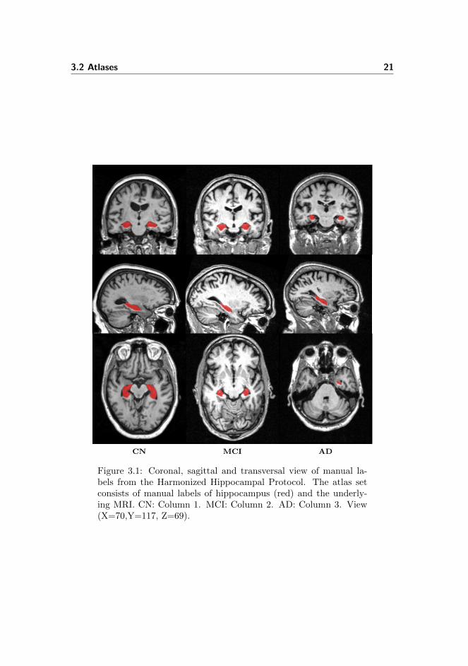
A subset of these manual annotations will serve as the atlas set in this thesis.These manual segmentations are chosen as atlas set in this work, because theyinclude both AD, MCI and CN of elderly subjects and they are as close as onecan get to a hippocampal segmentation golden standard. Since the labels havejust been made publicly available in August 2013, this work will be one of theinitial studies that evaluates how the labels perform as atlas set in state-of-the-art automated segmentation methods. The manual segmentations will be usedas atlas set in the two methods explained in Chapter 5. A coronal, sagittaland transversal view of a CN, MCI and AD subject is shown in Figure 3.1. Themanual hippocampus labels (red) are superimposed on the underlying MRI. Thecorresponding 3D illustrations of the manual labels can be seen in Figure 3.2.

20 Data and Atlases

Two different atlas sets are used in this thesis. Both sets are subsets of thereleased manual labels from the Harmonized Hippocampal Protocol (HHP). At-las15 includes 15 manual segmentations - these scans are not part of ADNI504.Atlas40 includes 40 manual segmentations, some of them are part of ADNI504.Information of each subject in these atlas sets can be found in Appendix A. Themean age, gender, MMSE score and hippocampal volume of the cognitive state(CN, MCI and AD) for the two atlas sets can be seen in Tables 3.2 and 3.3.


Age, yr ±σ 76.3 ± 7.9 72.7 ± 1.1 75.7 ± 8.0Men (%) 33.4 100 77.8MMSE ±σ 28.7 ± 1.0 27.0 ± 1.4 24.3 ± 2.8Volume (mm3)± σ 8127± 1240 7953 ± 1392 6952 ± 772

Table 3.2: Atlas15: Age, gender, MMSE score and hippocampalsize for CN, MCI and AD.


Age, yr ±σ 76.9 ± 6.2 70.9 ± 6.8 74.2± 8.6Men (%) 41.7 54.6 47.1MMSE ±σ 28.8 ± 1.2 27.6 ± 1.2 24.0 ± 2.7Volume (mm3)± σ 8176 ± 996 7708 ± 769 6887 ± 1080

Table 3.3: Atlas40: Age, gender, MMSE score and hippocampalsize for CN, MCI and AD.

3.2 Atlases 21

CN MCI AD

Figure 3.1: Coronal, sagittal and transversal view of manual la-bels from the Harmonized Hippocampal Protocol. The atlas setconsists of manual labels of hippocampus (red) and the underly-ing MRI. CN: Column 1. MCI: Column 2. AD: Column 3. View(X=70,Y=117, Z=69).

22 Data and Atlases

(a) CN (b) MCI (c) AD

Figure 3.2: 3D illustrations of the manual labels from Figure 3.1.

3.2.2 FreeSurfer atlas

Cross-sectional and longitudinal FreeSurfer will be used as reference methods inthis thesis. Both FreeSurfer methods uses the same probabilistic atlas, Chapter2. Therefore, it has not been possible to include Harmonized HippocampalProtocol atlases in this segmentation method, thus the hippocampal definitionin the FreeSurfer atlas is different than the atlas set used in BrainFuseLaband Non-Local Patch-based segmentation. 39 subjects are used to build theFreeSurfer atlas. They are a combination of healthy subjects as well as patientsof various ages with probable or questionable AD [4]. The atlas includes 37subcortical brain structures, and segmentations of all 37 structures are thusavailable. In this thesis, only hippocampal segmentations will be consideredand serve as a reference.

Chapter 4

Preprocessing

Due to large intensity differences in MRI, the test data and the training data(atlases) must be preprocessed before segmentation is carried out with the var-ious methods used in this thesis. Initially, the atlases and the preprocessedMRIs are not in the same space, thus they must be transformed to a commonspace prior to segmentation. Preprocessing will be explained in this chapter andinvolves:

1. MRI preprocessing (bias field correction and skull-stripping).

2. Transformation of atlas labels and preprocessed MRI to a common seg-mentation space.

4.1 MRI preprocessing

MRI preprocessing is done with FreeSurfer (v.5.1.0). Cross-sectional and longi-tudinal FreeSurfer segmentations are thus obtained from the same preprocessedimages as the segmentations obtained with the two methods explained in Chap-ter 5. This reduces the factors which can explain differences in segmentationresults.

24 Preprocessing

The first step is to conform the original MRI resolution, which is in the range[0.94, 1.35] × [0.94, 1.35] ×1.2 mm3, to isotropic voxels, 1 × 1 × 1 mm3. Theimage dimensions are changed to 256×256×256 voxels. During preprocessing,intensity normalization is done multiple times, where the MRI is scaled ac-cording to peak values within White Matter (WM), Grey Matter (GM) andCerebroSpinal Fluid (CSF).

4.1.1 Bias Field Correction

A MRI varies in both intensity and contrast across the 3D image. This spatialintensity inhomogeniety is called the bias field effect. The bias field effect isproportional to the scanners field strength and is caused by the Radio Frequencyfield inhomogeneities. Due to the bias fields effect, intra-class homogeneity cannot be assumed and accordingly identical tissue types will vary in intensitiesas a function of their spatial location. This is an undesirable condition for anysegmentation method, where intensity information is used to classify voxels intodifferent tissue types. The bias field effect is unique for each subject, whichmakes it challenging to correct it. FreeSurfer uses the non-parametric non-uniform intensity normalization, N3 [30], to correct for the bias field effect. Themethod is based on the following assumed model of MRI formation:

v(x) = u(x)f(x) + n(x) (4.1)

Where x is the location, v is the measured signal, u is the true signal, f isan unknown smoothly varying bias field, and n is white gaussian noise. Tocorrect for the bias field, f must be estimated. In Equation 4.1 the bias fieldis interfered by both an additive and multiplicative component, therefore, anoise-free additive model is used instead, with the notation u(x) = log(u(x)):

v(x) = u(x) + f(x) (4.2)

U ,V and F are the probability densities of u, v and f , respectively. u and f areapproximated uncorrelated random variables, and the distribution of their sumis found by convolution:

V (v) = F (v) ∗ U(v) =

∫F (v − u)U(u)du (4.3)

The task is to restore the frequency content of U , to get from the observed

4.1 MRI preprocessing 25

distribution V to the true distribution U . However, it is unknown which fre-quency components of U that need to be restored. The approach is to findthe smooth slowly varying field, f , that maximizes the frequency content of U .This is done by sharpening the distribution of V, estimate the correspondingf , which produces a distribution of U close to the one suggested. F is assumedto be Gaussian, having zero mean and a given variance, which means it is onlynecessary to search the space of distributions U corresponding to the propertiesof F. A MRI prior to and after bias field correction can be seen in Figure 1.5(a) and (b), respectively.

4.1.2 Skull-stripping

Whole-brain segmentation (skull-stripping) is an important discipline in analy-sis of neuroimaging data. During skull-stripping brain tissue is removed fromnon-brain tissue such as skull, eyeballs and skin. In FreeSurfer a watershed al-gorithm combined with a deformable model is used to peel the skull [29]. Twoassumptions are made:

1. Connectivity of WM is assumed, bordered by GM and CSF.

2. The brain surface, which distinguish non-brain from brain, is a smoothmanifold with relatively low curvature.

Before the watershed algorithm is applied, some parameters must be computed,these include an upper intensity bound for CSF, the centroid of the brain, anaverage brain radius, lower and upper bound for white matter intensity anda global brain minimum within a cubic region centered at the centroid of thebrain.

The watershed algorithm:Because white matter connectivity is assumed, WM surrounded by lower inten-sity GM and even lower intensity CSF in T1-weighted MRI, can be interpretedas a hill in a 3-dimensional landscape. By inverting the grey-scale values, theWM hill becomes a valley. The concept of pre-floating height is introduced.Prior to finding a connectivity path, each basin in the landscape is flooded upto a certain height above its bottom, the pre-floating height hpf . The defaultvalue of hpf is 25, corresponding to 25 % of the maximum intensity. If thepre-floating height is at a higher altitude than the the basin border, the basincannot hold water, and it will be merged with the deepest neighboring basin. Ifit holds water, it will be regarded as a separate region. Voxels are connected in apath, even if a lower intensity than the darkest of the two points are present up

26 Preprocessing

to a maximum difference, the pre-floating height. After the watershed transfor-mation has been applied, the segmented volumes still contain non-brain tissuesuch as CSF, some parts of the skull and often the entire brain-stem. The re-sult of the watershed algorithm can be seen in Figure 4.1. The output of thewatershed algorithm will serve as an initialization for a deformable model.

Figure 4.1: Before and after watershed transformation. The blackcross points out the centroid of the brain. White arrows indicatenon-brain regions, which have not been removed by the watershedtransformation [29].

Deformable surface algorithm:The segmented volume from the watershed algorithm is used to initialize adeformable balloon-like template using active contours. The initial brain surfacemodel is an icosahedron with 10242 vertices. This template is centered at thecentroid of the brain, with a radius that includes the whole previously segmentedbrain. The template is then gradually transformed through a series of iterativesteps. In each iteration the coordinate of each vertex is updated according tothree forces, a smoothness force Fs, a MRI-based force FMRI that drive thetemplate towards the true brain boundary and an atlas force FA that ensuresthe deformed template has the shape of a brain within a certain tolerance. Anexample of a deformation process can be seen in Figure 4.2. The deformedtemplate is then used to skull-strip the three dimensional MRI by removing thevoxels outside the estimated surface, 4.3.

4.2 Registration and label transformation 27

Figure 4.2: Template deformation process. Left: initial template(icosahedron). Right: Final template [9].

Figure 4.3: Final skull-stripping: Final deformed template (left)[29]. Middle and Right: Skull-stripped brain (red) superimposedon the original MRI

4.2 Registration and label transformation

The harmonized hippocampal standard manual segmentations are done by ex-pert operators in a standard space called MNI space. Prior to the manualsegmentation, the MRIs have been aligned to a template containing an averageof 152 brains in MNI space. This template can be seen in Figure 4.4

28 Preprocessing

Figure 4.4: Coronal, sagittal and transversal view of the MNI tem-plate found by averaging of 152 brains. Originally, the HHP atlasesare in this space. Image dimensions: 197×233×189.

To use the manual segmentations as atlases in the automated segmentationmethods, it is necessary to get them and the FreeSurfer preprocessed MRIs to acommon space. Since the preprocessed MRI is already in FreeSurfer space, thelabels will be taken to this space. This involves transforming labels from imagedimensions 197×233×189 to 256×256×256. The atlases will in this thesis bealigned using two different registrations. The first is a rigid-body transformation,whereas the other is an affine transformation.

Two steps are involved in registering a pair of images, registration and transfor-mation. In the registration, a set of parameters describing the transformationare estimated. In the transformation, one of the images is transformed accord-ing to the estimated parameters. Both the registration and transformation aredone using SPM [21],[2].

4.2.1 Rigid-Body Registration

Rigid-body or rigid transformations are a subclass of affine transformations. Foreach point in an image (x1, x2, x3) an affine mapping into the co-ordinates ofanother space (y1, y2, y3), can be represented as:

y1

y2

y3

1

=

m11 m12 m13 m14

m21 m22 m23 m24

m31 m32 m33 m34

0 0 0 1

x1

x2

x3

1

(4.4)


Rigid-body registrations consist of only translation and rotation and involvesestimating 6 parameters (3 for translation, 3 for rotation).

Translation: The translation of a point x by q units, is given by:y1

y2

y3

1

=

1 0 0 q1

0 1 0 q2

0 0 1 q3

0 0 0 1

x1

x2

x3

1

(4.5)

Rotation: The object can be rotated around three orthogonal planes (axes)in three dimensional images. Rotation matrices of q4, q5 and q6 radians aroundthe x-axis, y-axis and z-axis respectively are given by:

1 0 0 00 cos(q4) sin(q4) 00 −sin(q4) cos(q4) 00 0 0 1

,cos(q5) 0 sin(q5) 0

0 1 0 0−sin(q5) 0 cos(q5) 0

0 0 0 1

andcos(q6) sin(q6) 0 0−sin(q6) cos(q6) 0 0

0 0 1 00 0 0 1

(4.6)

Multiplication of these matrices combines rotations. The order of the multipli-cation influences the result.

4.2.2 Affine Registration

In affine transformation 12 parameters have to be estimated (3 translation, 3rotation, 3 scaling and 3 shearing). The translation and rotation is calculatedin the same way as described for rigid-body registration.

Scaling: Scaling is needed to change the size of the image. Scaling can berepresented as:

y1

y2

y3

1

=

q7 0 0 00 q8 0 00 0 q9 00 0 0 1

x1

x2

x3

1

(4.7)

Shear: Shear mapping by parameters q10, q11 and q12 are given by:

30 Preprocessing

y1

y2

y3

1

=

1 q10 q11 00 1 q12 00 0 1 00 0 0 1

x1

x2

x3

1

(4.8)

4.2.3 Optimization

Optimization is done to find the optimal parameters q. One image (sourceimage) is spatially transformed so it matches another image (reference image)by minimizing or maximizing some function or parameter. The usual approach isto do iteratively searching from an initial parameter estimate. At each iterationa judgement is made, before moving on to the next iteration. In both theaffine and rigid-body registrations, Gauss-Newton optimization is done basedon minimizing the sum of squared differences (SSD) dissimilarity measure.

The Gauss-Newton idea consists of linearizing the function (by Taylor expansionto first order). The parameters are updated by solving a set of linear equationsobtained from setting the first order derivatives equal to zero.bi(q) is the SSD describing the difference between the source and the referenceimage at voxel i, when the model parameters have values q. The method esti-mates the values of t in order to minimize

∑i bi(q− t)2. This is done from the

following sets of equations:

∂b1(q)∂q1

∂b1(q)∂q2

. .∂b2(q)∂q1

∂b2(q)∂q2

. .

. . . .

. . . .

t1t2..

'b1(q)b2(q)..

(4.9)

The parameters q are updated using an iterative scheme. For iteration n theparameters q are updated as:

q(n+1) = q(n) − (ATA)−1ATb (4.10)

where

A =

∂b1(q)∂q1

∂b1(q)∂q2

. .∂b2(q)∂q1

∂b2(q)∂q2

. .

. . . .

. . . .

,b =

b1(q)b2(q)..

(4.11)


This is repeated until SSD can no longer be decreased or a maximum of 64iterations is reached. However, the algorithm can be caught in a local minimumand therefore, there is no overall guarantee that the best global minimum iscalculated.

4.2.4 Transformation

Interpolation for each voxel in a transformed image is used to determine thecorresponding intensity in the original image. In this thesis, labels and imagesare interpolated using B-splines. B-splines are given by:

βn(x) =

n∑j=0

(−1)j(n+ 1)

(n+ 1− j)!j!max

(n+ 1

2+ x− j, 0

)n(4.12)

The degree, n, can be varied. n=0 corresponds to nearest neighbor interpola-tion, n=1 corresponds to trilinear interpolation and n=2 corresponds to cubicinterpolation. In nearest neighbor interpolation the original voxel intensities arepreserved. The value at each sample point is found by taking the value of theclosest voxel. Trilinear and cubic interpolation is slower than nearest neighborand uses the known intensities around the sample point to estimate the intensityat the sample point. The B-splines for n = 0, 1, 2 in 1-dimension is illustratedin Figure 4.5.

32 Preprocessing

(a) n=0. (b) n=1.

(c) n=2.

Figure 4.5: B-splines with different degrees of n found using Equa-tion 4.12. n=0: Nearest neighbor. n=1: Trilinear. n=2: Cubic.

The binary manual segmentations are transformed using nearest neighbor inter-polation, whereas the MRI is transformed using cubic interpolation. Trilinearinterpolation of the manual labels could have been an option, but this had in-volved determining an appropriate threshold to separate the transformed labelsinto object and background.

4.2.5 Illustrations

The atlases consist of manual segmentations and their corresponding MRI inMNI space. The same subjects are downloaded and preprocessed in FreeSurferand are then in subject FreeSurfer (FS) space. Thus, the MRI of the samesubjects are in two spaces.Transfer of manual segmentations to a common segmentation space involves acombination of an intra-subject and an inter-subject registration whereas theFreeSurfer preprocessed MRI is transformed using only the inter-subject regis-tration. The intra-subject registrations are always rigid-body transformations,whereas the inter-subject registration can be either a rigid-body transformationor an affine transformation. The registrations and transformations of MRIs andthe manual labels for subject 003 S 0931 are illustrated in Figures 4.6, 4.7 and4.8. The intra-subject registration, Figure 4.6, is done to find the transforma-


tion from MNI space to the the same subject in FS space registering originalMRI conformed to isotropic voxels. The inter-subject registration, Figure 4.7,is done to find the transformation from a subject in FS space to another subject(Atlas) in FS space registering preprocessed FreeSurfer Norm MRIs (bias cor-rected, skull-stripped and intensity normalized). Transformations T1 and T2,Figures 4.6 and 4.7, are combined in Figure 4.8 by:

T3 = T2(M/T1) (4.13)

If the labels are transferred from MNI space to Atlas FS space, Figure 4.8 , thenM is a transformation matrix that maps voxel coordinates from the isotropicMNI image to a space whose axes have parallel image axes, origin is at thecenter of the image and distances are measured in millimeters. M is given by:

M =

1 0 0 −DIM1/20 1 0 −DIM2/20 0 1 −DIM3/20 0 0 1

(4.14)

where DIM1, DIM2 and DIM3 are the image dimensions.

Figure 4.6: Intra-subject Registration using rigid-body reg-istration (illustrated by T1 arrow) between two different spaces.Result: Red channel - Transformed MRI using T1 transformationand cubic interpolation. Green channel - Target image.

34 Preprocessing

Figure 4.7: Inter-subject Registration using affine registra-tion (illustrated by T2 arrow) between two different spaces. Theregistration can also be a rigid-body registration. Result: Redchannel - Transformed Norm MRI using T2 transformation andcubic interpolation. Green channel - Target image (Norm MRI:bias corrected, intensity normalized and skull-stripped).

Figure 4.8: Label transfer combining T1 and T2 registrationsfrom Figures 4.6 and Figures 4.7. Hippocampus (red) is superim-posed on MRI in MNI space and on Norm MRI (bias corrected,intensity normalized and skull-stripped) in Atlas FS space.


Different combinations of the above illustrated transformations are used in thevarious segmentation methods in this thesis. However, in all cases, only onenearest neighbor interpolation is used to transfer the manual labels prior tosegmentation to avoid loosing to much information. The transfer of labels foreach segmentation method will be described in Chapter 5.

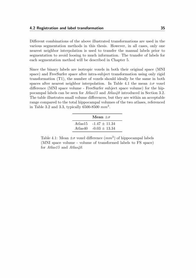
Since the binary labels are isotropic voxels in both their original space (MNIspace) and FreeSurfer space after intra-subject transformation using only rigidtransformation (T1), the number of voxels should ideally be the same in bothspaces after nearest neighbor interpolation. In Table 4.1 the mean ±σ voxeldifference (MNI space volume - FreeSurfer subject space volume) for the hip-pocampal labels can be seen for Atlas15 and Atlas40 introduced in Section 3.2.The table illustrates small volume differences, but they are within an acceptablerange compared to the total hippocampal volumes of the two atlases, referencedin Table 3.2 and 3.3, typically 6500-8500 mm3.

Mean ±σAtlas15 -1.47 ± 11.34Atlas40 -0.03 ± 13.34

Table 4.1: Mean ±σ voxel difference (mm3) of hippocampal labels(MNI space volume - volume of transformed labels to FS space)for Atlas15 and Atlas40.

36 Preprocessing

Chapter 5

Segmentation methods

Based on the content of Chapter 2, a multi-atlas Non-Local Patch-based seg-mentation method and a multi-atlas segmentation method using non-rigid reg-istrations are tested. The Non-Local Patch-based segmentation (N-L Patch)is implemented from scratch and can be found on the CD in Appendix C,whereas the multi-atlas segmentation using non-rigid registration (BrainFuse-Lab) is available for download. The atlases from the Harmonized HippocampalProtocol described in Chapter 3 will be used in both methods. Both methodsuse preprocessed images from FreeSurfer (bias field corrected, intensity normal-ized and skull-stripped) as explained in Chapter 4. This chapter describes thefundamental aspects of the segmentation methods.

5.1 Non-Local Patch-based segmentation

Segmentation is based on a Non-Local Patch-based framework using manualsegmentations as priors [8] [7]. These models do not need the computationalheavy non-rigid registrations, which are used in a majority of other multi-atlasapproaches and are therefore considerably faster.

A label is obtained for every voxel by using similar image patches from coarselyaligned atlases. When the patch under study resembles a patch in an atlas,

38 Segmentation methods

their central voxels are considered to belong to the same structure. The patchthat resembles the test patch is used in the estimation of the final label. Severalpatches from each atlas can be used during the label fusion of a single voxel,which increases the number of sample patches involved in the final label es-timation compared to other multi-atlas approaches where each atlas typicallyweights a voxel ones. The term non-local indicates that the spatial distancebetween the center of the patches is not taken into account. The weight of eachsample is solely depending on the intensity similarities between patches. Thesteps in the Non-Local Patch-based segmentation are explained below and canbe seen in Figure 5.2. The optimal parameters will be found in Chapter 6.

Linear registration to one atlas:Two sets of images need to be transformed to the same space, manual hippocam-pal labels and test MRI. The manual labels are transformed by combining T1and T2, as illustrated in Figure 4.8, Chapter 4. Initially, the MRIs are prepro-cessed in FreeSurfer space and therefore only T2 transformation is needed toget the MRI to the atlas segmentation space, Figure 4.7. Both a rigid as wellas an affine transformations are tried for T2, Chapter 6.

Initialization mask:Due to computational issues, the segmentation will only be applied to voxelsinside an initialization mask. The initialization masks are a union of the coarselyaligned atlases for left and right hippocampus, respectively.

Figure 5.1 illustrates three subjects registered with an affine registration to thesame space with the initialization mask overlaid (blue).

Figure 5.1: Three subjects registered to the same space with theinitialization mask overlaid (blue).

Subject selection:Due to computational cost, only a certain number of atlases, N , that resemblesthe subject under study the most, are used in the final non-local means labelfusion. The similarity based measure used is the sum of squared differences

5.1 Non-Local Patch-based segmentation 39

(SSD) across the initialization mask. SSD is used, because it is sensitive toe.g. contrast, which is an important factor in the label fusion. The subjectselection is done for left and right hippocampus separately, which means thatthe same atlas subjects not necessarily contribute to both the right and the lefthippocampus segmentation of a test subject.

Search volume:A search for similar patches should be done in the entire image under study.However, this is computationally expensive. Therefore, only a limited searchvolume, Vi, is used defined as a cube centered at the voxel under study, xi.Thus within the N closest selected atlases, the search for similar patches is ina cubic region around the voxel under study. The search volume must reflectthe inter-subject variability, which can increase when pathological changes arepresent, e.g. in AD, and according to the structure under study.

Preselection:In order to reduce the computational time, a preselection of patches are donediscarding the most dissimilar patches. The preselection criteria is based onsimple statistics such as mean and variance and can be seen below:

ss =2µiµs,jµ2i + µ2

s,j

× 2σiσs,jσ2i + σ2

s,j

(5.1)

where µ represents the means and σ represents the standard deviation of patchescentered on voxel xi (voxel under study) and voxel xs,j at location j in subjects. If the value of ss is higher than a given threshold, the intensity distancebetween patches in the non-local means label fusion is calculated by Equation5.3. The threshold is set to 0.95.

Non-local means label fusion:The non-local means estimator is used to perform a weighted average of thelabels based on the intensity distance between patches. The decision functionv(xi) is given by:

v(xi) =

∑Ns=1

∑j∈Vi

w(xi, xs,j)ys,j∑Ns=1

∑j∈Vi

w(xi, xs,j)(5.2)

where ys,j is the manual annotation given to voxel xs,j at location j in subjects. w(xi, xs,j) is the weight assigned to ys,j by patch comparison. The weight iscomputed as:

w(xi, xs,j) =

exp

−‖P (xi)−P (xs,j)‖22h2 if ss > th

0 else(5.3)

where P (xi) represents the cubic patch centered at xi and ‖ . ‖22 is the normal-ized L2 norm (normalized by the number of elements) computed between eachintensity element of patches P (xi) and P (xs,j).


If the labels are considered to be binary, 0 corresponding to background and 1to object, then:

L(xi) =

1 v(xi) > 0.50 v(xi) < 0.5

(5.4)

h in Equation 5.3 is the decay parameter. When h is low only a few samplesare taken into account, whereas a large value of h indicates that all sampleshave the same weight, and the estimation becomes a simple average. If patchesvery similar to the patch under study are estimated, h should be decreased toreduce the influence of other patches. When no similar patches are available,h should be increased to ensure that more patches are used in the label fusion.The estimation of h(xi) is done using:

h2(xi) = λ2 × arg minxs,j

‖ P (xi)− P (xs,j) ‖22 +ε (5.5)

where ε is a small constant to ensure stability in case the patch under study ispresent in the training data. λ=0.5 as proposed in [7].

Figure 5.2 illustrates the patch-based segmentation.

5.1 Non-Local Patch-based segmentation 41

Figure 5.2: Overview of the Non-Local Patch-based segmentation.Segmentation of voxel xi. The patch (green) is compared with allpatches within the search volume of the N closest subjects. Highestweights are obtained by the most similar patches (blue) [8].


5.2 BrainFuseLab

As described in Chapter 2, many multi-atlas segmentation methods exist. Inthis thesis, BrainFuseLab (BFL) is chosen [28]. A test image is registered witheach training subject using a diffeomorphic registration from ITK [16]. Usingthis transformation, the manual annotations are propagated to novel image co-ordinates approximately corresponding to the test subject’s coordinates. Labelfusion is reduced to a local weighted averaging, where training subjects that arelocally more similar to the test subject in terms of intensity get more weight.The method is developed to use bias field corrected, intensity normalized, skull-stripped images with isotropic voxels preprocessed in FreeSurfer as input. Theoriginal code uses an atlas set with several subcortical structures. Therefore,the code has been changed slightly since only hippocampal labels are availablein the HHP atlases.

Transfer of manual annotations:The MRI is preprocessed in FreeSurfer as described in Chapter 4. To get themanual labels to FreeSurfer space, a rigid-body registration, T1, is computed,as in illustrated in Figure 4.6. This transformation is used to move the manualsegmentations to FreeSurfer space using nearest neighbor interpolation.

Subject selection:Initially, all atlases are registered to the test subject using an affine registra-tion. Sums of squared differences (SSD) across an initialization mask (the skull-stripped brain mask) are calculated and the N closest subjects are selected. Theaffine parameters are saved and used later.

Non-rigid registration:The non-rigid registration is an ITK-based implementation of a Demon’s-basedregistration algorithm which can be found in [32]. In brief, this registrationscheme a stationary velocity field (SVF) setting where paths of diffeomorphismare generated using one parameter subgroups through the Lie group exponential.The Lie group exponential is realized through a series of self compositions ofa warp function. The warp Φ is parameterized with a smooth stationary fieldv : R3 7→ R3 via an Ordinary Differential Equation (ODE):

∂Φ(x, t)

∂t= v(Φ(x, t)) (5.6)

where the warp is defined as Φ(x) = exp(v)(x) with v being the velocity field.

Since the unidirectional registration is asymmetric due to the integral over dif-ferent volume forms, symmetry is ensured by transforming target volume form

5.2 BrainFuseLab 43

during the optimization using the Jacobian of the transformation. The follow-ing cost function is used to solve the variational problem to obtain an optimumvelocity field:

vn = arg minv

∑y∈Ω

[(I(y)− In(exp(v)(y))

]2+[(I(exp(−v)(y))− In(y)

]2det(∇exp(−v)(y))

+4λσ2∑

j,k=1,2,3

( ∂2

∂x2j

vk(x) |x=y

)2

(5.7)

where λ > 0 is the regularization parameter. xj and vk denotes the jth andkth dimension of the spatial position x, n is the nth training image, v is thevelocity, σ2 is the stationary noise variance, In denotes the N training imagesand In is the N training images where the spatial mapping from the test subjectcoordinates to the coordinates of the nth training images, Φn : Ω 7→ R3, isunknown. Regularization is achieved by convolving the velocity field updateswith a Gaussian: K(x) ∝ exp(−α

∑n=1,2,3 x

2i ), where α = γ/8λσ2 at every

optimization step. α determines the smoothness of the final warp and γ > 0controls the size of the Gauss-Newton step. Different values of γ are tried outin Chapter 6. Gauss-Newton scheme, section 4.2.3, is used to solve the ODE.

In Figure 5.3 a test subject and the corresponding closest training subject priorto and after warping the training image to the test image coordinates using thenon-rigid registration can be seen.


Test Training Test+Training

Test Warpedtraining

Test+Warped

Figure 5.3: Subject 003 S 0931 and the training image before(row1) and after warping (row2). Red channel: Test subject.Green channel: Training image.

Local Weighted Voting Label Fusion:The label fusion method is derived within a probabilistic framework. The goalis to estimate the label map L associated with the test image I, which can beachieved via a maximum-a-posterior (MAP) estimation.

L = arg maxL

p(L, I; Ln, In) (5.8)

Where In denotes the N training images with corresponding label maps Ln, n= 1,. . . ,N.

In the following M : Ω 7→ 1, . . . , N denotes the latent random field that foreach voxel in the test image I specifies the index of the training image In itwas generated from. The image I and the label map L can be generated from

5.2 BrainFuseLab 45

a mixture model, given a prior on M .

p(L, I; Ln, In) =∑M

p(M)p(L, I |M ; Ln, In) (5.9)

It is assumed that each voxel is generated from a single training subject in-dexed with M(x), i.e., p(L(x) | M ; Ln) = pM(x)(L(x);LM(x)) and p(I(x) |M ; In) = pM(x)(I(x); IM(x)). Inserting this into 5.9 gives:

p(L, I; Ln, In) =∑M

p(M)∏x∈Ω

pM(x)(L(x);LM(x))pM(x)(I(x); IM(x)) (5.10)

The final cost function is achieved by substituting 5.10 into 5.8:

L = arg maxL

∑M

p(M)∏x∈Ω

pM(x)(L(x);LM(x))pM(x)(I(x); IM(x)) (5.11)

Equation 5.11 has 3 individual terms, image likelihood (pM(x)(I(x); IM(x))),label prior (pM(x)(L(x);LM(x))) and membership prior p(M). Variations inthese terms gives different label fusion strategies.

For local weighted voting, M(x) is independent and identically distributed ac-cording to an uniform distribution over all labels for all x ∈ Ω, which means themembership prior becomes:

p(M) =1

N |Ω|(5.12)

This reduces Equation 5.11, with L denoting the number of labels includingbackground, to:

L(x) = arg maxl∈1,...,L

N∑n=1

pn(L(x) = l;Ln)pn(I(x); In) (5.13)

The image likelihood serves as weights and is modeled as a Gaussian distributionwith stationary variance σ2:

pn(I(x); In) =1√

2πσ2exp[− 1

2σ2

(I(x)− In(Φn(x))

)2](5.14)


The label prior term serves as votes and is given by:

pn(L(x) = l;Ln) =1

L∑l=1

(ρDl

n(Φn(x)))exp(ρDl

n(Φn(x)))

(5.15)

where In is N training images where the spatial mapping from the test subjectcoordinates to the coordinates of the nth training images, Φn : Ω 7→ R3, isunknown. Dl

n denotes the distance transform of label l in training subject n. ρis a slope constant.

Chapter 6

Parameter and methodselection

To find the best method to segment ADNI504, the appropriate parameters usedin Non-Local Patch-based segmentation (N-L Patch) and BrainFuseLab mustbe found. To find these parameters, leave-one-out cross-validation is done. Inleave-one-out cross-validation (LOOCV) one single observation from a datasetis used as test data, and the remaining observations are used as training data.This is repeated until each observation in the dataset is used once as test data.Due to computational cost, LOOCV will initially be done on 15 atlases, Atlas15.When the appropriate parameters have been found, LOOCV will be done usingAtlas40. ADNI504, Atlas15 and Atlas40 are explained in Chapter 3. Throughthis chapter cross-sectional FreeSurfer will be used as reference. LongitudinalFreeSurfer segmentations are not available for the atlases - only one time pointscan is available for some of the atlases. Based on LOOCV, one method willbe selected to segment ADNI504 and atrophy will be estimated and comparedto cross-sectional and longitudinal FreeSurfer in Chapter 7. To compare thedifferent methods and parameters, a volume overlap measure known as Dicescore is used to evaluate the quality of the segmentations. Given an automaticsegmentation L and the corresponding manual segmentation L, the Dice scoreof label l is given by [28]:

48 Parameter and method selection

Dice(l; L, L) = 2|x ∈ Ω|L(x) = l&L(x) = l|

|x ∈ Ω|L(x) = l|+ |x ∈ Ω|L(x) = l|(6.1)

where Ω ⊂ R3 is a finite grid where the test subject is defined. The Dicescores varies between 0 and 1, where 0 indicates 0 % overlap with the manualsegmentation and 1 indicates 100 % overlap with the manual segmentation -thus a perfect segmentation.

6.1 Atlas15 - Leave-one-out cross-validation

LOOCV with 15 atlases will be done on both N-L Patch and BrainFuseLab tofind the appropriate parameters. These parameters will be applied in a LOOCVof Atlas40 in Section 6.2. The parameter annotation is the same as used inChapter 5.

6.1.1 Non-Local Patch-based segmentation

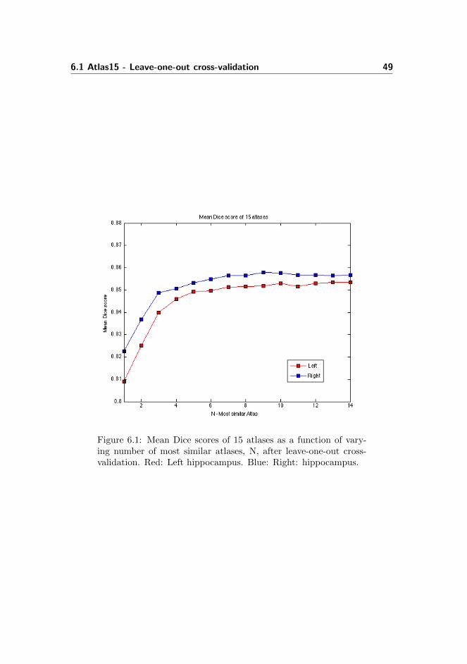
N closest subjects:Initially, a rigid-body registration is used to do both the intra- and inter-subjectregistration to one of the atlases in the atlas dataset, Figures 4.6 and 4.7. Thelabels and MRIs are transformed using the calculated transformation. Thenumber of N closest atlases found under pre-selection can be varied from 1to 14. The patch size and the search volume are set to 7×7×7 and 9×9×9,respectively, as suggested in [8]. Figure 6.1 illustrates mean Dice score aftersegmentation of 15 atlases as a function of a varying number of most similaratlases, N, from 1 to 14 after LOOCV. Dice scores are shown for both left andright hippocampus.

6.1 Atlas15 - Leave-one-out cross-validation 49

Figure 6.1: Mean Dice scores of 15 atlases as a function of vary-ing number of most similar atlases, N, after leave-one-out cross-validation. Red: Left hippocampus. Blue: Right: hippocampus.


Figure 6.1 illustrates that after using approximately N=9 closest atlases in thesegmentation, a steady state is reached. Therefore, N=9, will be used in N-LPatch.

Search volume and patch size:The search volume (sv) can be viewed as the inter-subject variability of thestructure. Since the hippocampus has a large variability, especially in patholog-ical brains, one would expect that the search volume should be large comparedto other structures with less variability. 3 different search volumes with sidelength 9, 11 or 13 are tested. For each search volume, 3 different patch sizes(ps) with side length, 3, 5 or 7 are tested. The Dice scores for left and righthippocampus with varying parameters can be seen in Table 6.1. N=9 closestsubjects are used in the segmentation. The approximate segmentation compu-tation duration in minutes per subject is shown in the table as well (Time).

Search Volume 9Patch size 3 5 7

Dice score left ±σ 0.829 ± 0.027 0.856 ± 0.026 0.853 ± 0.028Dice score right ±σ 0.836 ± 0.032 0.863 ± 0.027 0.858 ± 0.030Time (min) 32 40 80





Table 6.1: Search volume and patch size impact on Dice score. Apatch size of e.g. 3 corresponds to a 3×3×3 volume. Dice scores forleft and right hippocampus as well as the duration of segmentingboth left and right hippocampus for one subject can be seen.

Based on both precision in terms of Dice score and time, a patch volume of sidelength 5 and a search volume of side length 9 will be used.

Affine vs. rigid registration:The inter-subject registration can be done using a rigid-body registration or


an affine registration, Figure 4.7. To test the impact on the precision, bothregistrations are tried out in LOOCV, Figure 6.2. Mean Dice scores are denotedby the horizontal line in the figure and can be seen in Table 6.2 as well.

(a) Right (b) Left

Figure 6.2: Dice scores as a function of atlas number. Segmentationof the 15 atlases using inter-subject rigid registration (red) or affineregistration (blue). LOOCV using N=9, sv=9, ps=5. Mean Dicescores are denoted by the horizontal line.

Mean Dice score ±σRight Left

Affine 0.875±0.019 0.867±0.017Rigid 0.863±0.026 0.856±0.025

Table 6.2: Mean Dice scores of LOOCV using 15 atlases wherelabels are aligned using affine or rigid registration.

Since an affine registration results in both a larger mean Dice score and a smallerstandard deviation, Table 6.2, than using a rigid registration, affine registrationwill be used to do the inter-subject registration to transform labels and MRIs.

Align labels to test subject or standard atlas:Two different ways in aligning the atlases and test subject to a segmentationspace have been tested. Dice scores as a function of atlas number can be seen inFigure 6.3. In Figure 6.3 (a), both the test subject and the atlases are alignedto the first atlas in the atlas set, atlas1 (Affine to atlas1), blue. In Figure 6.3(b), all the atlases are aligned to the test subject (Affine to subject), red. The


corresponding mean Dice scores are denoted by the horizontal line and is statedin Table 6.3.

(a) Right (b) Left

Figure 6.3: Dice scores as a function of atlas number. Red: Testsubjects and atlases are all aligned to atlas1 using affine registra-tion (affine to atlas1). Blue: Atlases are aligned to the test subjectusing affine registration (affine to subject).

Mean Dice score ±σRight Left Time (min)

Affine to atlas1 0.875±0.019 0.867±0.017 40Affine to subject 0.876±0.018 0.868±0.017 60

Table 6.3: Mean Dice scores of LOOCV using 15 atlases where la-bels are aligned using affine transformation to either atlas1 (Affineto atlas1) or the test subject (Affine to subject). Furthermore, thecomputation time of segmenting both left and right hippocampusin a subject is stated (Time).

As Figure 6.3 and Table 6.3 illustrates, doing the inter-subject registration ofall atlases to atlas1 once or doing the registration of all atlases to the testsubject, gives the same results. Aligning all atlases to atlas1 only has to be doneonce. Segmentation of a new test subject then only requirers one registration,which takes the test subject’s coordinates to atlas1’s coordinates. This approachis considerably faster than aligning all atlases to the test subject each time.Therefore, aligning to atlas1 will be used onwards.


Threshold of non-local means estimator:According to [8], the threshold of the non-local means estimator v(xi), Equation5.4, decides if a voxel belongs to the object (L=1) or the background (L=0).This threshold is suggested to be 0.5 in [8]. To verify if this is the optimal valuefor this implementation, the threshold of v(xi) is varied from 0 to 1, which leadsto a number of slightly different segmentations. The total Dice score (both leftand right hippocampus) with the manual segmentations are calculated. Theplot of Dice scores as a function of the threshold of v(xi) can be seen in Figure6.4.

Figure 6.4: Dice scores as a function of varying threshold v(xi) ofAtlas15. Each curve illustrates the behavior of one atlas.

The maximum Dice score and the corresponding threshold v(xi)max of eachatlas is found. The 15 v(xi)max have a mean value of 0.42. This results in amean Dice score of 0.875. A threshold of 0.5 as suggested in [8] results in a meanDice score of 0.871. Since it is only the 3. decimal that is affected by changingthe threshold from 0.42 to 0.5, a threshold of 0.5 will be used as suggested in[8].

Removal of small connected components:Many segmentations have speckle patterns (black) as illustrated in row 2 inFigure 6.5. Therefore, a modification of the original method is made. Connectedcomponents are found using a 6-connectivity neighborhood and are removed iftheir total volume is less than 100 voxels. The Dice scores, before and after


removal can be seen in Table 6.4. The table indicates, that the removal doesnot affect Dice scores. However, a visually more satisfying result is achievedafter removal, row 3 Figure 6.5, and therefore a removal of small connectedcomponents will be performed on top of N-L Patch.

Mean Dice score±σRight Left

Before removal 0.875±0.019 0.867±0.017After removal 0.875±0.019 0.868±0.017

Table 6.4: Mean Dice scores of LOOCV using 15 atlases before andafter removing connected components with volumes less than 100voxels.

6.1.2 BrainFuseLab

BrainFuseLab has many parameters that can be varied in wide ranges, Section5.2. According to [28] it is especially the following parameters which affectthe result: γ that controls the step size in the gauss-newton optimization, andthe standard deviation σ in the Gaussian Image Likelihood term used for labelfusion, Equation 5.14. To make a fair comparison with N-L Patch, N=9 closestatlases will be used. The settings in the downloaded demo (γ = 20, σ = 5)and the default values (γ = 150, σ = 10), have been tested. LOOCV using thedefault and demo parameters can be seen in Figure 6.6. Notice, that the y-axishas been changed due to very low Dice-scores compared to Figure 6.3. Themean Dice scores ±σ can be seen in Table 6.5.


Manual segmentations

Before removal of Connected Components

After removal of Connected Components

Figure 6.5: 3D illustrations of removal of connected components(black, row 2) from two subjects left and right column respec-tively. Top: Manual segmentations. Middle: Segmentations (red)with connected components < 100 voxels (black). Bottom: Afterremoval of connected components.


(a) Right (b) Left

Figure 6.6: Dice scores as a function of atlas number. BrainFuse-Lab LOOCV with demo parameters (red) and default parameters(blue).


Mean Dice score ±σRight Left

Demo parameters 0.798±0.025 0.775±0.043Default parameters 0.763±0.066 0.765±0.058

Table 6.5: Mean Dice scores of LOOCV with BrainFuseLab. Demoparameters and default parameters are tested.

Based on these findings, the demo parameters will be used further on.

6.2 Atlas40 - Leave-one-out cross-validation

25 extra atlases are introduced and LOOCV is done. The optimal parametersfound using Atlas15 are used to do N-L Patch segmentation as well as segmen-tation with BrainFuseLab (BFL). As suggested as future work in e.g. [8], thenon-rigid registration from BrainFuseLab are combined with N-L Patch. Thetransformed labels for N closest atlases using BrainFuseLab are collapsed intoa mask that serves as initialization mask for N-L Patch. The segmentation ofboth left and right hippocampus is done using the N closest atlases found inBrainFuseLab.The Dice scores with the manual HHP labels, false positive error (FP) and falsenegative error (FN) with N-L patch, BFL, combination of non-rigid registrationfrom BFL and N-L patch (Non rigid + N-L Patch) and cross-sectional FreeSurfer(FS Cross) can be seen Table 6.6. Furthermore, a box plot of the Dice scores ofthe different methods can be seen in Figure 6.7. When calculating Dice scores,there has not been distinguished between right and left hippocampus as donein most of section 6.1.Notice that the number of atlases and number of closest atlases are fundamen-tally different for cross-sectional FreeSurfer, Table 6.6. Cross-sectional FreeSurferuses a probabilistic atlas build from 39 atlases as explained in Section 3.2.2,which means averaged information from all these atlases are used in the seg-mentation. The FreeSurfer Dice scores are obtained by calculating the overlapof segmentations with the HHP labels, even though FreeSurfer uses anotheratlas to do segmentation with a different definition of hippocampus. By do-ing this, the FreeSurfer segmentation consensus with the new label standard isillustrated.


Method Atlas NMean Dicescore ±σ Mean FP ±σ Mean FN ±σ

N-L Patch 40 9 0.868 ± 0.019 0.125 ± 0.025 0.138 ± 0.028BFL 40 9 0.827 ± 0.027 0.139 ± 0.040 0.203 ± 0.034Non rigid +N-L Patch

40 9 0.857 ± 0.016 0.106 ± 0.021 0.177 ± 0.023

FS Cross 39 - 0.781 ± 0.031 0.158 ± 0.030 0.270 ± 0.052

Table 6.6: Atlas40 LOOCV. Atlas: Number of atlases availableduring preselection based on SSD. N closest: Number of closestatlases based on SSD used in segmentation. FP: False Positiveerror. FN: False negative error.

Figure 6.7: Box plot of the Dice scores with different methods.Boxes represents the lower quartile, the median (red line) andthe upper quartile. Whiskers indicate the extreme values within 1times the interquartile range. Outliers (red +) are the data valuesbeyond the end of the whiskers.


As seen in Table 6.6, the best mean Dice score is achieved using N-L patch.However, the mean Dice score is approximately the same as the one achievedusing 15 atlases (mean Dice score = 0.871). On the other side, the mean Dicescore has increased for BFL. This indicates, that N-L patch due to the factthat it can use more than one similar patch from each atlas, do not need asmany available atlases in order to perform well as methods that only uses in-formation once for each atlas to segment a voxel. It should further be noticed,that combining the non-rigid registration from BrainFuseLab and N-L patch in-creases the Dice score compared to BFL from a mean of 0.827 ± 0.027 to 0.857± 0.016. This illustrates N-L Patch’s label fusion capabilities compared to thelocal weighted voting label fusion used in BrainFuseLab.

The approximate computation times can be seen in Figure 6.7. The codes areall a single core CPU implementation on a 2.5 GHz Xeon.

Method Computational time (hours)N-L Patch ∼ 0.7BFL ∼ 5Non rigid + N-L Patch ∼ 5.5FS Cross ∼ 11

Table 6.7: Computational times for each subject with differentmethods. It should be noticed that FS Cross segments 37 subcor-tical structures incl. the hippocampi, whereas the other methodsonly segments two: left and right hippocampus.

Statistics:Paired t-tests between methods based on Dice scores from LOOCV using 40atlases have been made independent of CN, MCI and AD, Table 6.8. The p-values are < 0.001 for N-L patch vs. all other methods, which according to thenull hypothesis means that equal means can be rejected.

Methods t-value p-valueN-L Patch vs. FS Cross 27.6346 <0.001N-L Patch vs. BFL 13.5424 <0.001N-L Patch vs. Non rigid + N-L Patch 7.6142 <0.001BFL vs. FS Cross 12.9467 <0.001BFL vs. Non rigid + N-L Patch -9.892 <0.001FS Cross vs. Non rigid + N-L Patch -21.1403 <0.001

Table 6.8: Results of paired t-tests between Dice scores of differentmethods.


Illustrations:Based on the FreeSurfer segmentations, the worst, median and best atlas subjectis selected. The segmentations of these three subjects segmented using differentmethods are illustrated in a coronal, sagittal and transversal view, Figures 6.8,6.9 and 6.10. Notice, that in order to illustrate the N-L Patch segmentationsin the same segmentation space as the other methods, they must be takenback to the subjects FreeSurfer space, by applying the inverse transformation,T2−1, from Figure 4.7. This involves a nearest neighbor interpolation. Due tothis interpolation, the mean Dice score changes from 0.868 ± 0.019 to 0.855 ±0.021. However, as illustrated in Table 4.1 this only changes volume size a little.Hippocampal volume size will be used to calculated atrophy. Furthermore, the3D segmentations of the worst, median and best subject can be seen in Figure6.11.

From Figures 6.8, 6.9, 6.10 and 6.11 it can be seen that both N-L Patch andthe non-rigid registration combined with N-L Patch, visually look most likethe manual segmentations (green). This is also reflected in the Dice scoresachieved with these methods. The FreeSurfer segmentations are rough, whereasthe BranFuseLab segmentations have some speckles after segmentation both atthe hippocampal borders as well as within the background labels.


Figure 6.8: Worst subject 002 S 0938 (AD)

Manual segmentation

FreeSurfer. Dice = 0.696

BrainFuseLab. Dice = 0.766

Non-rigid registration + N-L Patch. Dice = 0.822

N-L Patch. Dice = 0.821


Figure 6.9: Median subject 013 S 1276 (CN)

Manual segmentation






Figure 6.10: Best subject 011 S 0002 (CN)

Manual segmentation






Manual segmentations

Dice=0.696 Dice=0.788 Dice=0.827

FreeSurfer

Dice=0.766 Dice=0.847 Dice=0.867

BrainFuseLab

Dice=0.822 Dice=0.874 Dice=0.874

Non-rigid registration + N-L Patch

Dice=0.821 Dice=0.871 Dice=0.875

N-L Patch

Figure 6.11: 3D illustrations of left: Worst subject. Middle: Me-dian subject. Right: Best subject. Selected based on FreeSurferLOOCV results.

6.3 Evaluation 65

6.3 Evaluation

N-L Patch results in Dice scores significantly higher than all other methodsusing paired t-tests between methods independent of diagnostic groups, Table6.8. Furthermore, N-L Patch is the fastest method. Therefore, N-L Patch willbe implemented in Chapter 7.

Even though Dice scores are not improved by using 40 atlases compared to 15,40 atlases will be used since this increases the library used for atlas preselec-tion. Furthermore, the computation time is not increased more than a coupleof minutes using 40 atlases compared to 15 atlases, since the time is dependingmost on the number of N closest atlases used in segmentation.

In [8] the best mean Dice score is reported to be 0.884. However, this scoreis from LOOCV of 80 healthy young subjects (mean age: 25.09 ± 4.9 years)and N=30 closest subjects. In this work a mean Dice score of 0.868 is achievedfrom LOOCV of 40 subjects with pathological processes (mean age: 74.10±7.67years) and N=9 closest subjects. The two numbers cannot directly be comparedsince it is more difficult to segment brains of elderly people with pathologicalprocesses then healthy young subjects due to large variability in the subjects.

Combining the non-rigid registration from BrainFuseLab with N-L Patch resultsin a mean Dice score of 0.857 ± 0.016 compared to BrainFuseLab with a meanof 0.827 ± 0.027. This indicates that the label fusion technique in N-L Patchis better than the technique used in BrainFuseLab. Whether this is due to amore comprehensive parameter optimization in N-L Patch or the fact that N-LPatch also uses information from shifted voxels is hard to tell. Figure 6.12 illus-trates the histogram of one subject inside the manual hippocampal mask (left)and the corresponding histogram of the most similar atlas image (right) aftertransformation of the atlas using the non-rigid registration in BrainFuseLab.Large differences can not be observed between the histograms. This indicatesthat the mediocre results obtained with BrainFuseLab cannot be explained bythe non-rigid registration.


(a) Test (b) Warped

Figure 6.12: Histogram inside hippocampusmask. Left: Test sub-ject. Right: Most similar warped atlas after non-rigid registration.

Chapter 7

Final results

In Chapter 6, Non-Local Patch-based segmentation (N-L Patch) was found tobe the most optimal method based on both precision (Dice scores) and com-putation time. Therefore, N-L Patch will be used to segment ADNI504 at 3time points, month 0 (baseline), month 12 (m12) and month 24 (m24). Atrophywill be estimated between baseline-month 12 (bam12) and baseline-month 24(bam24). Since manual segmentations are only available for very few MRIs inADNI504, no segmentation ground truth is available for the entire dataset, andDice scores cannot be calculated. The evaluation of the method will be based onits diagnostic group separation capabilities compared to current methods usedat Biomediq A/S, cross-sectional FreeSurfer and longitudinal FreeSurfer.

In this chapter, adjustments in preprocessing, inter-subject registration andskull-stripping, is done for some subjects to achieve the final segmentationsof ADNI504. Using the final segmentations, atrophy will be estimated and astatistical analysis will be made to evaluate the diagnostic group separation ca-pabilities of N-L Patch compared to cross-sectional FreeSurfer and longitudinalFreeSurfer. Finally, the results are discussed.

In this thesis, longitudinal FreeSurfer segmentations are calculated exploitingtwo time points simultaneously (baseline and m12 or baseline and m24) to seg-ment one time point. This means, that the baseline volume used to calculatebam12 is not the exact same as the baseline volume used to calculate bam24.

68 Final results

7.1 Method

N-L Patch segmentation of ADNI504 is done with search volume = 9, patchsize = 5, number of atlases = 40, N closest atlases = 9 using an affine inter-subject registration to one atlas as suggested in Chapter 6. 21 atlases in Atlas40are also part of ADNI504. When these 21 subjects are segmented their atlasis not used in the segmentation. Since a segmentation of one subject takesabout 40 minutes, the total computation time used to segment all subjects wasapproximately 1000 hours.After the initial segmentation, the hippocampal volume is estimated. If the totalsubject hippocampal volume is below 3500 voxels, a rigid-body inter-subjectregistration is done instead of the affine and the segmentation is done again. Asegmentation volume of 3500 voxels is considered to correspond to an extremelyinsufficient segmentation, since the total hippocampal volume typically is 6500-8500 mm3, as referenced in Table 3.2 and 3.3.Since rigid registrations does not involve shearing and scaling, the registrationsare not as sensitive to e.g. insufficient skull-strippings or enlarged ventricles asaffine registrations. However, applying a rigid registration does not give goodresults in all cases. If segmentation is still very poor (total hippocampal volumebelow 3500 voxels and visual inspection) the preprocessed MRIs are inspected.In all cases, the poor results were due to an insufficient skull-stripping. Theskull-stripping is changed by adjusting the watershed parameter, Section 4.1.2,until the MRI is correctly separated into brain tissue and non-brain tissue. Theinitial segmentation using affine registration is done again. Table 7.1 indicatesthe number of times the registration is changed or skull-stripping is redone toachieve the final results for ADNI504 at baseline, m12 and m24, respectively.After fixing the skull-stripping good results were achieved in all cases.

Rigid Skull-strip

Baseline 6 0m12 12 3m24 12 4

Table 7.1: Number of times registration fails and either a rigidregistration is done or the skull-stripping is fixed. Rigid: If thetotal hippocampus volume was below 3500 voxels after the initialsegmentation, then the inter-subject registration was changed toa rigid registration and the segmentation was done again. Skull-strip: If the result still was not satisfying after a rigid registration,the skull-stripping was changed and the segmentation was doneagain.

7.1 Method 69

Figure 7.1 illustrates the MRI of subject 109 S 1114 m12 before and after fix-ing an insufficientt skull-stripping and Figure 7.2 illustrates the correspondingsegmentations.

Initial skull-stripping

Final skull-stripping

Figure 7.1: Coronal, sagittal and transversal view of subject109 S 1114 m12 before (row1) and after (row2) an insufficient skull-stripping has been fixed.

70 Final results

Figure 7.2: Hippocampal segmentation of subject 109 S 1114 m12before (left) and after (right) an insufficient skull-stripping hasbeen fixed, Figure 7.1.

To achieve the final segmentations, affine inter-subject registration was usedfor most subjects, whereas rigid inter-subject registration was used for a mi-nority of subjects when the affine registration failed. Since affine registrationinvolves scaling, the results achieved using an inter-subject affine registrationcannot volumewise be compared to the results achieved using an inter-subjectrigid registration. Thus, all segmentations are transformed back to the subject’sFreeSurfer space, by applying the inverse transformation, T2−1, from Figure 4.7,before the the total segmentation volume is estimated.

7.2 Segmentation results

The sum of voxels (1 voxel = 1mm3) for all 504 subjects at baseline, m12and m24 for N-L patch, cross-sectional FreeSurfer and longitudinal FreeSurfercan be found on the CD in Appendix C. The corresponding volume box plotswith the three methods at baseline can be seen in Figure 7.3 for AD, MCIand CN. The longitudinal volumes are calculated exploring baseline and m12simultaneously. The mean ± σ can be seen in Table 7.2. A corresponding ta-ble containing m12 and m24 mean ±σ for diagnostic groups with N-L Patch,cross-sectional FreeSurfer and Longitudinal FreeSurfer can be seen in AppendixB. Furthermore, scatter plots of baseline hippocampal volume with N-L Patchagainst cross-sectional FreeSurfer, Figure 7.4, and N-L Patch against longitu-dinal FreeSurfer, Figure 7.5, can be seen. The scatter plots for N-L patch vs.cross-sectional FreeSurfer and longitudinal FreeSurfer for m12 and m24 can be

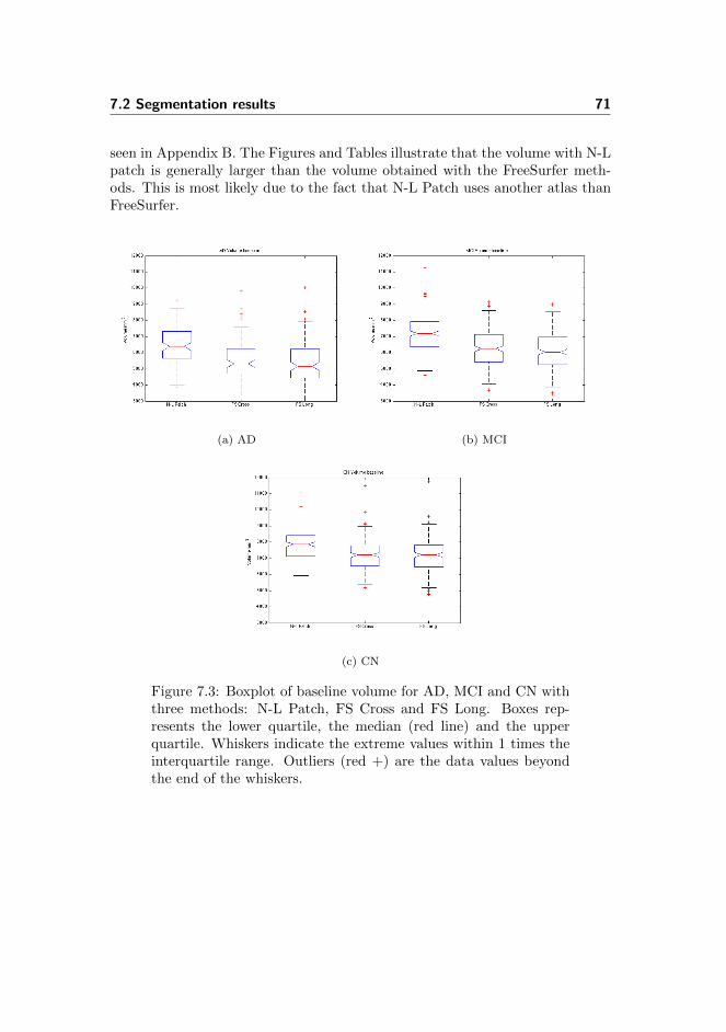
7.2 Segmentation results 71

seen in Appendix B. The Figures and Tables illustrate that the volume with N-Lpatch is generally larger than the volume obtained with the FreeSurfer meth-ods. This is most likely due to the fact that N-L Patch uses another atlas thanFreeSurfer.

(a) AD (b) MCI

(c) CN

Figure 7.3: Boxplot of baseline volume for AD, MCI and CN withthree methods: N-L Patch, FS Cross and FS Long. Boxes rep-resents the lower quartile, the median (red line) and the upperquartile. Whiskers indicate the extreme values within 1 times theinterquartile range. Outliers (red +) are the data values beyondthe end of the whiskers.

72 Final results

Volume (mm3)± σCN(n=169) MCI(n=234) AD(n=101)

N-L Patch 7860 ± 880 7166 ± 1083 6520 ± 1190FS Cross 7210 ± 968 6313 ± 1263 5569 ± 1216FS Long 7168 ± 1026 6117 ± 1083 5356 ± 1277

Table 7.2: ADNI504 baseline: Hippocampal volume for diagnosticgroups with different methods.

Figure 7.4: ADNI504 baseline: Hippocampal volume. N-L Patchvs. FS Cross.

7.3 Statistical analysis 73

Figure 7.5: ADNI504 baseline: Hippocampal volume. N-L Patchvs. FS Long.

7.3 Statistical analysis

Based on the volume results, atrophy rate is estimated as percentage volumechange from baseline to m12 (bam12) and baseline to m24 (bam24).

atrophy(%) =(Follow-up volume

Baseline volume− 1)∗ 100 (7.1)

The corresponding atrophy histograms with 50 bins for N-L Patch, cross-sectionalFreeSurfer and longitudinal FreeSurfer can be seen in Appendix B. The segmen-tations of a MCI subject, 130 S 0783, with N-L Patch at baseline, m12 and m24can be seen in Figure 7.6. Bam12 atrophy = -2.15 % and bam24 atrophy =-7.53 %. The subject is diagnosed with MCI at all 3 time points.

74 Final results

(a) Baseline (b) m12 (c) m24

Figure 7.6: Segmentation of subject 130 S 0784 (MCI) with N-LPatch at baseline (volume = 7234 mm3), m12 (volume = 7044mm3) and m24 (volume = 6689 mm3). Bam12 atrophy = -2.15 %and bam24 atrophy = -7.53 %.

Figure 7.6 illustrates the difficulty in visually seeing differences in volume be-tween time points, even for this MCI subject with pathological changes in thebrain.

Based on the atrophy scores, a statistical analysis will be made to evaluatethe diagnostic group separation capabilities of N-L Patch compared to cross-sectional and longitudinal FreeSurfer. The statistical analysis of each methodbetween diagnostic groups are done by performing two sample t-tests, AUCs andCohen’s Ds. Furthermore, an analysis between methods are done by comparingCohen’s Ds and AUCs. Bootstrapping is used to compare Cohen’s Ds betweenmethods, whereas DeLong test is used to compare AUCs between methods.

Initially, Bartlett’s test of variance inhomogeneity is made and can be foundin Appendix B. The low p-values reveal variance inhomogeneity between theclinical diagnostic groups in N-L Patch and longitudinal FreeSurfer for bothbam12 and bam24 and cross-sectional FreeSurfer bam24. Variance homogeneitycannot be rejected for cross-sectional FreeSurfer bam12. This will be considered,when performing two sample t-tests between groups. The statistics calculatedbased on atrophy bam12 and bam24 can be seen in Tables 7.3 and 7.4. A briefanalysis of the results will be given in the following sections.


AD MCI CN

mean ±σ mean ±σ mean ±σN-L Patch -4.23 ±3.06 -2.39 ±3.28 -0.86 ±2.46FS Cross -4.29 ±5.32 -3.69 ±5.48 -1.39 ±5.41FS Long -4.83 ±3.74 -3.25 ±3.53 -1.63 ±2.54

AD vs. CN AD vs. MCI MCI vs. CN

t-test (p-value) t-test (p-value) t-test (p-value)

N-L Patch -9.36 (<0.001) -4.93 (<0.001) -5.33 (<0.001)FS Cross -4.67 (<0.001) -0.92 (0.357) -4.16 (<0.001)FS Long -8.35 (<0.001) -3.69 (<0.001) -5.08 (<0.001)


AUC (p-value) AUC (p-value) AUC (p-value)

N-L Patch 0.80∗∗ (<0.001) 0.66∗∗∗ (<0.001) 0.65 (<0.001)FS Cross 0.69 (<0.001) 0.53 (0.404) 0.67 (<0.001)FS Long 0.76 (<0.001) 0.62 (<0.001) 0.64 (<0.001)


Cohens’D Cohens’D Cohens’D

N-L Patch 1.21∗∗∗ 0.58∗∗ 0.53FS Cross 0.54 0.11 0.42FS Long 1.00 0.44 0.53

Table 7.3: Statistics based on atrophy (%) of ADNI504 betweenbaseline and month 12. The first value for each t-test is the t-value.N-L Patch: DeLong test is done to compare AUCs between meth-ods and bootstrapping is done to compare Cohens’ Ds betweenmethods. ** indicates significance of N-L Patch over FS Crosswith p-value: 0.001≤p-value<0.01; and *** indicates significanceof N-L Patch over FS Cross with p-value<0.001.

76 Final results

AD MCI CN



t-test (p-value) t-test (p-value) t-test (p-value)

N-L Patch -10.60(<0.001) -5.16 (<0.001) -7.28 (<0.001)FS Cross -7.96 (<0.001) -2.81 (0.005) -6.94 (<0.001)FS Long -12.71 (<0.001) -4.87 (<0.001) -8.98 (<0.001)


AUC (p-value) AUC (p-value) AUC (p-value)

N-L Patch 0.86 (<0.001) 0.69∗ (<0.001) 0.71 (<0.001)FS Cross 0.82 (<0.001) 0.62 (<0.001) 0.73 (<0.001)FS Long 0.89 (<0.001) 0.67 (<0.001) 0.73 (<0.001)


Cohens’D Cohens’D Cohens’D

N-L Patch 1.43∗ 0.62∗ 0.70FS Cross 1.04 0.34 0.69FS Long 1.69 0.57 0.87

Table 7.4: Statistics based on atrophy (%) of ADNI504 betweenbaseline and month 24. The first value for each t-test is the t-value. DeLong test is done to compare AUCs between methods andbootstrapping is done to compare Cohens’ Ds between methods.* indicates significance of N-L Patch over FS cross with p-value,0.01≤p-value<0.05.

Two sample t-tests:For each method, two sample t-tests between two diagnostic groups at a timeis performed to test the hypothesis:

H0 : µ1 − µ2 = 0

H1 : µ1 − µ2 6= 0(7.2)

Based on the results of Bartlett’s test, Appendix B, only variance homogeneitybetween groups will be assumed for cross-sectional FreeSurfer bam12. The t-values and p-values can be seen in Tables 7.3 and 7.4. Cross-sectional FreeSurferAD vs. MCI bam12 is the only test, that is not significant. Thus there is asignificant difference in atrophy rates for all other test scenarios.


AUC:Area Under a ROC Curve (AUC) is defined as the area under a Receiver Oper-ating Characteristics (ROC) graph. ROC graphs are commonly used in medicaldecision making to visualize a classifiers performance. The curve is achieved bychanging the threshold of the measure which is evaluated, and for each thresh-old, calculate the false positive rate (x-axis) and the true positive rate (y-axis).(0,1) corresponds to a perfect classification. y=x represent randomly guessinga class. AUC will always be between 0 and 1, but since 0.5 corresponds torandom guessing, no realistic classifier should be below 0.5 [11]. A ROC curvewith corresponding AUC value can be seen in Figure 7.7. The remaining ROCcurves can be seen in Appendix B. All AUC scores with corresponding p-valuesare stated in Tables 7.3 and 7.4. All combinations of diagnostic groups with thedifferent methods are significant except cross-sectional FreeSurfer bam12 ADvs. MCI. Here, only an AUC of 0.52 is achieved, which almost corresponds torandom guessing. To compare AUCs between methods (derived from the samesubjects between diagnostic groups), DeLong test is used [10]. The test takesinto account the correlated nature of the data. N-L Patch AUCs are comparedto cross-sectional FreeSurfer and Longitudinal FreeSurfer. Significance betweenmethods, indicated by *, ** and *** in Tables 7.3 and 7.4, are found for N-Lpatch and cross-sectional FreeSurfer bam12 for diagnostic groups AD vs. CNand AD vs. MCI and bam24 AD vs. MCI. No significant difference is foundbetween N-L Patch and longitudinal FreeSurfer.

Figure 7.7: ROC curve. AD vs. CN for N-L Patch bam12. Truepositive rate vs. false positive rate as a function of the thresholdof the measure that is evaluated.

78 Final results

Cohens’ D:Cohens’ D is a measure of effect size which indicates the strength of a phe-nomenon. It is defined as the difference between two means, µ1 and µ2, dividedby a measure based on the standard deviations, σ1 and σ2, for the data.

Cohens′D =µ1 − µ2√σ21+σ2

2

2

, (7.3)

Cohens’ D are correlated with another statistical measure typically used in drugtesting, sample size. A low Cohens’ D indicates the necessity of a larger samplesize. Bootstrapping is used to compare Cohens’ Ds between methods. To com-pute the p-value for bootstrapping, a two-tailed t-test for the null hypothesisof equal measures N1-N2=0 is carried out, where N1 and N2 are independentrandom measures. A probability distribution is computed for the differencebetween the Cohens’ D for the two measures and computes the p-value asp(N1 > N2) = 1 − cdfN1−N2(0) and p(N2 > N1) = 1 − p(N1 > N2), wherecdf is the cumulative distribution function.

N-L Patch Cohen’s Ds are compared to cross-sectional FreeSurfer and Longi-tudinal FreeSurfer. Significance between methods, indicated by ** and *** inTable 7.3 and by * in Table 7.4, are found for N-L patch and cross-sectionalFreeSurfer bam12 and bam24 for diagnostic groups AD vs. CN and AD vs.MCI. No significant difference is found between N-L Patch and longitudinalFreeSurfer.

7.3.1 Linear regression

In the following model, it is assumed that the hippocampal percentual loss peryear is constant. This means that the volume loss is an exponentially decayingfunction. To find the rate, a straight line is fitted by least squares estimates[23] to three points calculated as log(Follow-up volume/Baseline volume). Atbaseline, the follow-up volume is equal to the baseline volume, accordingly, thefirst point is always 0. The best fitted exponential line to the three target pointsis found, where best is defined by the least squares estimates. The fitted linesfor the three methods can be seen in Figures 7.8, 7.9 and 7.10.


Figure 7.8: N-L Patch: Blue dots: Volume, (log(follow-up/baseline)), as a function of scan interval. Grey lines: Best fittedlines to three time points using least squares estimates. Black line:Mean.

Figure 7.9: FS Cross: Blue dots: Volume, (log(follow-up/baseline)), as a function of scan interval. Grey lines: Best fittedlines to three time points using least squares estimates. Black line:Mean.

80 Final results

Figure 7.10: FS long: Blue dots: Volume, (log(follow-up/baseline)), as a function of scan interval. Grey lines: Best fittedlines to three time points using least squares estimates. Black line:Mean.

The rate per year for each subject is found by:rate (%) = (exp(slope coefficient) - 1)*100. The mean rate for each diagnosticgroup with N-L Patch, cross-sectional FreeSurfer and longitudinal FreeSurfercan be seen in Table 7.5.

AD MCI CN


Table 7.5: Statistics based on rate/year for ADNI504. The rateis found by fitting a straight line to 3 time points calculated aslog(follow-up volume / baseline volume) using least squares esti-mates.

From Figures 7.8, 7.9 and 7.10 it can be seen that the deviation looks largerfor cross-sectional FreeSurfer than N-L Patch and longitudinal FreeSurfer. Ac-cording to the model, the lines found by least squares estimates should intersect

7.4 Discussion 81

(0,0). To test for bias, a two sided one sample t-test is used to test if the linesintersections with the y-axis for each method is equal to zero. The result of thetest can be seen in Table 7.6.

One sample t-test

N-L Patch FS Cross FS Long

t-vale (p-value) -0.79 (0.432) 0.46 (0.649) 2.19 (0.029)

Table 7.6: Two sided one sample t-test for each method based onthe intersection with the y-axis of best fitted straight lines to threetime points using least squares estimates. Volume is defined aslog(Volume Follow-up/Volume Baseline).

From Table 7.6 it can be seen, that the null hypothesis, µ = 0, can be rejectedfor FS long. This can be due to bias, uncertainties in measurements or a wrongmodel assumption - the hippocampal volume is not an exponentially decayingfunction.

7.4 Discussion

As stated in Section 7.2, the initial segmentations are insufficient in some cases(total volume below 3500 voxels). It is not unusual that inter-subject registra-tions fail, since large intensity differences between subjects can lead to a scenariowhere the optimization can be caught at a local minimum as explained in Chap-ter 4. However, when the skull-stripping is changed, the segmentations are goodin all cases. This could indicate the need to inspect all the skull-stripped im-ages prior to segmentation or simply use another type of preprocessed images,e.g. bias field corrected images. The argumentation for using skull-strippedimages in the first place is that the registration is not dominated by the highintensity skull, thereby resulting in a better hippocampal alignment. A precisehippocampal alignment is important to achieve good segmentation results sinceN-L Patch only search for similar patches within a 9×9×9 voxels search volume.Therefore, changing the input images to bias field corrected images might notimprove registration and thereby segmentation.

Segmentation with N-L Patch is in the same space after an affine inter-subjectregistration, since all atlases and subjects are registered to one atlas. However,when the inter-subject registration is changed to a rigid registration to the same

82 Final results

atlas, no scaling and shearing is done, which means the segmentations results areavailable in another space. Thus, the segmentations cannot directly be comparedin these cases, and must be taken to a standard space. Furthermore, doing acomparison with the other methods involves taking the segmentations to subjectFreeSurfer space and doing an interpolation. This affects Dice scores with themanual labels, which changes from 0.868 ± 0.019 to 0.855 ± 0.021 for Atlas40,Chapter 6. This could be avoided if a computational heavier alternative wasused where atlases were registered to the test subject, as done in BrainFuseLaband Section 6.1.1, and might accordingly be considered in future work.

From Tables 7.3 and 7.4 it can be seen that the standard deviations for N-LPatch is increased for bam24 compared to bam12. This can be due to moreextreme outliers which can be seen from the histograms in Appendix B. Theseoutliers are not corrected, since the total hippocampal volume is not below 3500voxels. Figure 7.11 illustrates a segmentation where the left hippocampus of anAD subject, indicated by blue arrow, is not segmented properly, which leads toa atrophy score from baseline to m24 of -31 %. The left hippocampus volumedecreases from 3867 to 1906 mm3, whereas the right decreases from 4562 to3909 mm3. Since the left and right hippocampus should have approximatelythe same volume, the fraction between the volumes could have been used as anindicator to decide if the MRI should be inspected for e.g. an imprecise skull-stripping. Figure 7.12 illustrates the transformed MRI, green, superimposed onthe test atlas, greyscale. In this case, it does not look like a faulty registration.More likely, it is not possible to use affine registration to match the brain of thissubject, because the pathological brain changes are very large, e.g. enlargedventricles.

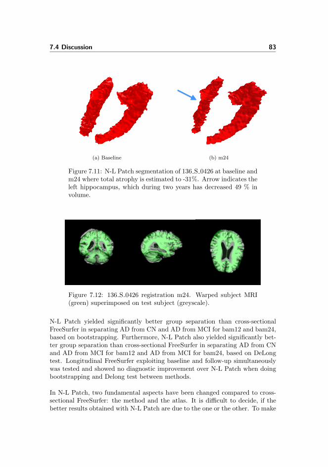
7.4 Discussion 83

(a) Baseline (b) m24

Figure 7.11: N-L Patch segmentation of 136 S 0426 at baseline andm24 where total atrophy is estimated to -31%. Arrow indicates theleft hippocampus, which during two years has decreased 49 % involume.

Figure 7.12: 136 S 0426 registration m24. Warped subject MRI(green) superimposed on test subject (greyscale).

N-L Patch yielded significantly better group separation than cross-sectionalFreeSurfer in separating AD from CN and AD from MCI for bam12 and bam24,based on bootstrapping. Furthermore, N-L Patch also yielded significantly bet-ter group separation than cross-sectional FreeSurfer in separating AD from CNand AD from MCI for bam12 and AD from MCI for bam24, based on DeLongtest. Longitudinal FreeSurfer exploiting baseline and follow-up simultaneouslywas tested and showed no diagnostic improvement over N-L Patch when doingbootstrapping and Delong test between methods.

In N-L Patch, two fundamental aspects have been changed compared to cross-sectional FreeSurfer: the method and the atlas. It is difficult to decide, if thebetter results obtained with N-L Patch are due to the one or the other. To make

84 Final results

a fair comparison, the methods should preferably use the same atlas. However,since there is no access to the atlases used to build the probabilistic FreeSurferatlas, this has not been possible.The new Harmonized Hippocampal Protocol (HHP) label definition is madeby many experts after evaluating a variety of segmentation protocols and thenagreeing on an equivocal definition. This suggests that the manual HHP seg-mentations are more standardized and thereby better than the manual segmen-tations used in FreeSurfer. Furthermore, HHP labels are considered the newhippocampal golden standard. The cross-subject averaging done to make theFreeSurfer atlas might have removed useful information. On the other hand,the FreeSurfer atlas has been used for a long time, and the atlases used to makethis probabilistic atlas are used in other automated multi-atlas methods as welle.g. [28], which illustrates their robustness in automated segmentation.

FreeSurfer and N-L Patch methods are fundamentally different. FreeSurfer usesMarkov Random Fields in a Baysian framework to do segmentation. Infor-mation from intensity, prior probabilities at a voxel and labels of neighboringvoxels, is included in the model.In its original form, the N-L patch method results in segmentations with specklepatterns, as illustrated in Section 6.1. These areas are wrongly classified aspart of hippocampus because the method does not take labels of neighboringclassified voxels into account. However, the speckles can easily be removed au-tomatically as done in this thesis. The segmentations obtained using FreeSurferare often rough and has branches of misclassified voxels, Figure 1.7. Since thesebranches are not represented in the FreeSurfer atlas, they arise because of themethod. The branches are interconnected with the hippocampus border andcan only be removed by morphological operations, which effects the entire sur-face volume. Since the surface volume accounts for approximately 10 % of thetotal volume, this is not an optimal solution when estimating atrophy.

N-L Patch only uses affine registrations or the subclass, rigid registrations, andis therefore considerably faster than methods using non-linear registration. Nogeneral rule exist, but methods that uses a lot computational power are oftenmore precise than methods that use less. The question is if N-L Patch onlyperforms well because a good atlas from the HHP is available? In [8], N-LPatch is used for ventricle segmentation with another atlas and gives good re-sults. Segmentation of 80 elderly subjects with mild to moderate AD gives amean Dice score = 0.959. This indicates the possibility to extend the methodto other structures. However, the computational cost increases with structuresize. To make N-L Patch even faster in order to get segmentation results im-mediately after the scan, the images could be cropped and the method could beimplemented on a GPU.

Chapter 8

Conclusion

The ambition behind this thesis was to improve automated segmentation of hip-pocampus from T1-weighted Magnetic Resonance Imaging (MRI) compared tothe current method (FreeSurfer) used at the company Biomediq A/S. BiomediqA/S strives at eliminating the use of FreeSurfer in their alzheimer’s diagnosticpipeline.

In an initial literature study, multi-atlas segmentation methods were found tobe among the top performing automated hippocampal segmentation methods.These methods rely on manual annotations called atlases. Two fundamentallydifferent multi-atlas methods were chosen, to analyze if the best performancewas achieved with 1) the relatively faster N-L Patch using affine registrationsto align MRIs and atlases or with 2) a computationally heavier method, Brain-FuseLab, using non-rigid registrations to align atlases and MRIs. In N-L Patcha label is obtained for every voxel by using similar image patches from coarselyaligned atlases, whereas BrainFuseLab gives atlases with local similarity to thetest subject high weight when a voxel is labeled. For both methods, manualannotations from a new Harmonized Hippocampal Protocol (HHP) were usedas atlases. These manual annotations include both subjects with alzheimer’sdisease (AD), mild cognitive impairment (MCI) and cognitively normal (CN),and are furthermore considered the hippocampal golden standard.

Before segmentation the MRI data were preprocessed in several steps for both

86 Conclusion

methods. This involved removal of spatial intensity inhomogeneities, skull-stripping and transformation of atlases and MRIs to one segmentation space.

Method parameters were optimized in a leave-one-out cross-validation using twodifferent HHP atlas sets. A paired t-test between Dice scores of N-L Patch andBrainFuseLab, showed significance (p<0.001), accordingly N-L Patch yieldedsignificantly higher Dice scores than BrainFuseLab. This illustrates, that heavycomputational methods not necessarily give better results than fast methods.Based on Dice scores, computation time and visual inspection, N-L Patch waschosen to be the optimal method. Furthermore, N-L Patch resulted in bettersegmentation consensuses with the new hippocampal label standard than thestate-of-the-art method, cross-sectional FreeSurfer.

N-L Patch was used to segment a standardized ADNI dataset containing 1.5TMRIs from 504 subjects (169 CN, 234 MCI, 101 AD) at baseline, month 12and month 24. In cases, where the registration was considered to fail, either theskull-stripping was redone or the registration was changed to a rigid registrationas it was considered that the scaling caused the fail. After these adjustments, noinsufficient segmentations were achieved with hippocampal volume below 3500mm3.

Hippocampal atrophy rate calculated as percentage volume change from base-line to follow-up was estimated. Based on a statistical analysis, the diagnosticgroup separation capabilities of N-L Patch were compared to two state-of-the-artmethods, 1) cross-sectional FreeSurfer and 2) longitudinal FreeSurfer. Includingthe HHP labels in N-L Patch yielded significantly better group separation thancross-sectional FreeSurfer in separating AD from CN and AD from MCI. Alsolongitudinal FreeSurfer exploiting baseline and follow-up simultaneously showedno diagnostic improvement over N-L Patch. This illustrates the longitudinal ro-bustness of segmentations when annotations from the new hippocampal labelstandard are included in automated segmentation methods.

Two fundamentally different aspects were changed in N-L Patch compared to theFreeSurfer methods: the method and the atlas. The definition of the HHP labelshave been agreed upon by many experts, which indicates that the atlases used inN-L Patch are better than the probabilistic atlas used in FreeSurfer, where theaveraging of atlases might have removed usefull information. Based on the visualsegmentations, both N-L Patch and FreeSurfer have areas of misclassified voxels.However, in N-L Patch these can easily be removed since they are not part ofthe hippocampal border which is not the case in FreeSurfer. This indicates, thatthe method used in N-L Patch results in better automated segmentations thanFreeSurfer.

Based on the results of this thesis, Biomediq A/S now has achieved a fast

8.1 Future Work 87

hippocampal segmentation method independent of the segmentation part ofFreeSurfer. Additionally, Biomediq A/S now has a method with full access tothe source code. However, the use of FreeSurfer is not eliminated as the MRIsstill need to be preprocessed. Developing a preprocessing pipeline might be con-sidered in future work, if the use of FreeSurfer should be eliminated completely.If atlases are available for other subcortical structures, the N-L Patch methodcan easily be extended to segment such structures as well. A GPU implementa-tion will decrease computation time further, with high clinical relevance, sincesegmentations should preferably be available in the clinic immediately afterscanning.

Overall, hippocampal N-L Patch segmentation with HHP labels showed con-vincing results, though, there is still room for improvements and new featuresin the segmentation.

8.1 Future Work

Below is a list with possible elements for improving hippocampal N-L Patchsegmentations and steps in getting a better subcortical segmentation pipeline.

1. Include a similarity measure based on texture analysis of the test andtraining subjects in the non-local means label fusion, Equation 5.2.

2. If many similar patches are found from the same training subject, it in-dicates that this subject globally looks like the test subject. This couldbe incorporated in the label fusion, so patches from that specific trainingsubject weights more in the final fusion of labels, Equation 5.2.

3. Optimize N-L patch code by cropping images around the structure ofinterest and make a GPU implementation.

4. Extent the method to other structures. This involves finding good atlassets.

88 Conclusion

Appendix A

Atlas Demographics

This appendix includes the demographics of the manual segmentations from theHarmonized Hippocampal Protocol used as atlas sets in this thesis. One atlasset contains 15 atlases, Table A.1, the other contains 40 atlases, Table A.2.MMSE score is explained in Chapter 3.

PatientID SeriesID Diagnosis Age Gender MMSE Hand002_S_0816 29.612 AD 71,4630 1 26 1 Gender MMSE hand003_S_0931 20.050 CN 86,2247 2 28 1 1 26 1003_S_1059 22.301 AD 84,5616 2 25 1 2 28 1003_S_1257 27.340 AD 85,1342 1 20 1 2 25 1009_S_0842 18.870 CN 73,7151 1 28 1 1 20 1009_S_0862 19.358 CN 73,4685 2 30 1 1 28 1009_S_1030 21.823 MCI 67,5507 1 28 1 2 30 1009_S_1334 50.567 AD 64,8767 1 22 1 1 28 1011_S_0002 9.107 CN 74,3863 1 28 2 1 22 1013_S_0592 18.419 AD 78,1370 1 23 1 1 28 2013_S_1276 27.641 CN 71,9644 2 30 1 1 23 1016_S_1092 23.826 MCI 74,4685 1 26 1 2 30 1016_S_1263 27.304 AD 64,8822 2 26 1 1 26 1100_S_1062 66.023 AD 84,4712 1 28 1 2 26 1100_S_1286 64.890 CN 77,7205 2 28 2 1 28 1

2 28 2

15 pers7 AD6 CN2MCI

Figure A.1: Atlas15 demographics. Gender: Male = 1, female =2. Hand: Right = 1, left = 2.

90 Appendix A

PatientID SeriesID Diagnosis Age Gender MMSE Hand002_S_0295 13.408 CN 84,8904 1 28 1002_S_0413 13.893 CN 76,3836 2 29 1002_S_0782 17.835 MCI 81,7205 1 29 1002_S_0816 29.612 AD 71,4630 1 26 1002_S_0938 19.852 AD 82,3068 2 23 1003_S_0907 19.728 CN 88,7260 2 30 1003_S_0908 32.516 MCI 62,9616 2 29 1003_S_0931 20.050 CN 86,2247 2 28 1003_S_1057 23.345 MCI 61,3753 2 26 1003_S_1059 22.301 AD 84,5616 2 25 1003_S_1122 23.542 MCI 76,8055 2 28 1003_S_1257 27.340 AD 85,1342 1 20 1005_S_1341 27.673 AD 71,7151 2 24 1007_S_0101 10.679 MCI 73,6356 1 27 1007_S_0128 10.936 MCI 64,1288 2 29 1009_S_0842 18.870 CN 73,7151 1 28 1009_S_0862 19.358 CN 73,4685 2 30 1009_S_1030 21.823 MCI 67,5507 1 28 1009_S_1334 50.567 AD 64,8767 1 22 1010_S_0067 10.344 CN 74,5562 1 27 1011_S_0002 9.107 CN 74,3863 1 28 2011_S_0010 8.800 AD 73,9699 2 24 1011_S_0016 9.253 CN 65,4630 1 28 1011_S_0183 12.000 AD 72,5452 2 21 1011_S_0856 19.031 AD 60,3781 1 27 2013_S_0592 18.419 AD 74,0000 1 28 1013_S_1276 27.641 CN 71,9644 2 30 1016_S_1092 23.826 MCI 74,4685 1 26 1016_S_1263 27.304 AD 64,8822 2 26 1098_S_0149 11.021 AD 87,8137 1 20 1098_S_0172 11.812 CN 70,6384 2 29 1100_S_0995 66.038 AD 81,0548 2 26 1100_S_1062 66.023 AD 84,4712 1 28 1100_S_1286 64.890 CN 77,7205 2 28 2123_S_0050 10.053 MCI 77,7233 1 26 2123_S_0091 15.898 AD 62,9616 1 25 1123_S_0094 15.867 AD 71,3014 2 20 1123_S_1300 27.689 MCI 73,5452 2 28 2127_S_0259 12.137 CN 70,6301 1 30 1127_S_0754 18.515 AD 67,7123 2 23 1

Figure A.2: Atlas40 demographics. Gender: Male = 1, female =2. Hand: Right = 1, left = 2.

Appendix B

Statistical Analysis

The results in this appendix are obtained from a statistical analysis of the finalsegmentations from ADNI504 with Non-Local Patch-based segmentation (N-LPatch), cross-sectional FreeSurfer (FS cross) and longitudinal FreeSurfer (FSlong) explained in Chapter 7.

B.1 Volume results

Tables B.1 and B.2 states the mean ±σ for N-L Patch, cross-sectional FreeSurferand longitudinal FreeSurfer for the diagnostic groups at m12 and m24, respec-tively. The corresponding baseline table is Table 7.2. Since one patient is notdiagnosed at m24, the results are obtained using the baseline diagnostics.

92 Appendix B

Mean volume (mm3)± σCN(n=169) MCI(n=234) AD(n=101)

N-L Patch 7792 ± 889 6996 ± 1096 6247 ± 1182FS Cross 7107 ± 1018 6075 ± 1110 5330 ± 1197FS Long 7055 ± 1052 5921 ± 1173 5105 ± 1276

Table B.1: ADNI504 m12: Mean hippocampal volume for diagnos-tic groups with different methods.

Mean volume (mm3)± σCN(n=169) MCI(n=234) AD(n=101)

N-L Patch 7716± 908 6850 ± 1149 6034 ± 1223FS Cross 6985 ± 1014 5869 ± 1161 5049 ± 1195FS Long 6918 ± 1059 5702± 1220 4817 ± 1253

Table B.2: ADNI504 m24: Mean hippocampal volume for diagnos-tic groups with different methods.

Scatter plots of N-L Patch volume against cross-sectional FreeSurfer or longitu-dinal FreeSurfer at m12 and m24 can be seen in Figures B.1 and B.2, respec-tively. The corresponding figures for baseline can be seen in Figures 7.4 and7.5. Since one patient is not diagnosed at m24, the results are obtained usingthe baseline diagnostics.

B.1 Volume results 93

Figure B.1: ADNI504 m12: Scatter plots. Top: Hippocampalvolume with N-L Patch vs. FS Cross. Bottom: Hippocampalvolume with N-L Patch vs. FS Long.

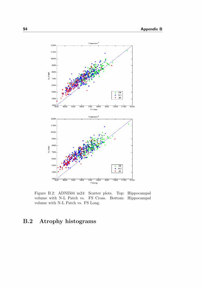
94 Appendix B

Figure B.2: ADNI504 m24: Scatter plots. Top: Hippocampalvolume with N-L Patch vs. FS Cross. Bottom: Hippocampalvolume with N-L Patch vs. FS Long.

B.2 Atrophy histograms

B.2 Atrophy histograms 95

(a)

N-L

Patc

hb

am

12.

(b)

FS

Cro

ssb

am

12.

(c)

FS

Lon

gb

am

12.

(d)

N-L

Patc

hb

am

24.

(e)

FS

Cro

ssb

am

24.

(f)

FS

Lon

gb

am

24.

Fig

ure

B.3

:F

requ

ency

vs.

per

centa

ge

diff

eren

cein

hip

poca

mp

al

volu

me

(atr

op

hy)

bet

wee

nb

ase

lin

ean

dfo

llow

up

(bam

12or

bam

24)

wit

hd

iffer

ent

met

hod

s.

96 Appendix B

B.3 Bartlett’s Test

To test for variance homogeneity between groups, Bartlett’s test, is performedon atrophy rates for the three diagnostic groups, AD, MCI and CN for eachmethod. The results of Bartlett’s test are shown in Tables B.3 and B.4. The lowp-values reveal variance inhomogeneity between the clinical diagnostic groups inN-L Patch method and longitudinal FreeSurfer for both bam12 and bam24 andcross-sectional FreeSurfer bam24. Variance homogeneity can not be rejected forcross-sectional FreeSurfer bam12.

Segmentation Method p-valueN-L Patch <0.001FS Cross 0.9469FS Long <0.001

Table B.3: Bartlett’s tests of inhomogeneity of variances bam12.

Segmentation Method p-valueN-L Patch <0.001FS Cross 0.007FS Long <0.001

Table B.4: Bartlett’s tests of inhomogeneity of variances bam24.

B.4 ROC curves

ROC curves for bam12 and bam24 with corresponding AUC values can be seenin Figures B.4 and B.5.

B.4 ROC curves 97

(a)

N-L

Patc

hA

Dvs.

CN

.(b

)N

-LP

atc

hA

Dvs.

MC

I.(c

)N

-LP

atc

hM

CI

vs.

CN

.

(d)

FS

Cro

ssA

Dvs.

CN

.(e

)F

SC

ross

AD

vs.

MC

I.(f

)F

SC

ross

MC

Ivs.

CN

.

(g)

FS

Lon

gA

Dvs.

CN

.(h

)F

SL

on

gA

Dvs.

MC

I.(i

)F

SL

on

gM

CI

vs.

CN

.

Fig

ure

B.4

:R

OC

curv

esb

am

12.

98 Appendix B

(a)

N-L

Patc

hA

Dvs.

CN

.(b

)N

-LP

atc

hA

Dvs.

MC

I.(c

)N

-LP

atc

hM

CI

vs.

CN

.

(d)

FS

Cro

ssA

Dvs.

CN

.(e

)F

SC

ross

AD

vs.

MC

I.(f

)F

SC

ross

MC

Ivs.

CN

.

(g)

FS

Lon

gA

Dvs.

CN

.(h

)F

SL

on

gA

Dvs.

MC

I.(i

)F

SL

on

gM

CI

vs.

CN

.

Fig

ure

B.5

:R

OC

curv

esb

am

24.

Appendix C

Data CD

The enclosed CD contains the following:

• Volume results of ADNI504 at 3 time points with N-L Patch, FS cross andFS long.

• Atrophy scores of ADNI504 (bam12, bam24) with N-L Patch, FS crossand FS long.

• N-L Patch source code.

• R-code and m-code used for statistics.

Bibliography

[1] P. Aljabar, R.A. Heckemann, A. Hammers, J.V. Hajnal, and D. Reuckert.Multi-atlas based segmentation of brain images: Atlas selection and itseffect on accuracy. Neuroimage, 46:726–738, 2009.

[2] John Ashburner and Karl. J. Friston. Rigid body registration. in: statisticalparametric mapping: The analysis of functional brain images. AcademicPress, pages 49–62, 2007.

[3] Dubois B, Feldman HH, Jacova C, DeKosky ST, , Delacourte A Barberger-Gatteau P, Cummings J, Galalsko D, Gauthier S, Jicha G, Meguro K,O’Brian J, Pasquier F, Robert P, Rossor M, Salloway S, Stern Y, Visser Pj,and Scheltens P. Research criteria for the diagnosis of alzheimer’s disease:revising the nincds-adrda criteria. Lancet Neuron, 43(6):734–746, 2007.

[4] Fischl B, Salat DH, Busa E, Albert M, Dieterich M, Haselgrove C, van derKouwe A, Killiany R, Kennedy D, Klaveness S, Montillo A, Makris N,Rosen B, and Dale AM. Whole brain segmentation: automated labelingof neuroanatomical structures in the human brain. Neuron, 33(3):341–355,2002.

[5] Kolawole Oluwole Babalola, Brian Patenaude, Paul Aljabar, Julia Schn-abel, David Kennedy, William Crum, Stephen Smith, Tim Cootes, MarkJenkinson, and Daniel Rueckert. An evaluation of four automatic meth-ods of segmenting the subcortical structures in the brain. Neuroimage,47:1435–1447, 2009.

[6] Marie Chupin, Emilie Gerardin, Remi Cuignet, Claire Boutet, LouisLemieux, Stephane Leheicy, Habib Benali, Line Garnero, Olivier Colliot,

102 BIBLIOGRAPHY

and the Alzheimers Disease Neuroimaging Initiative. Fully automatic hip-pocampus segmentation and classification in alzheimer’s disease and mildcognitive impairment applied on data from adni. Hippocampus, 19(6):579–787, 2009.

[7] Pierrick Coupe, Simon F. Eskildsen, Jose V. Manjon, Vladimir Fonov,D. Louis Collins, and the Alzheimer’s Disease Neuroimaging Initiative. Si-multaneous segmentation and grading of anatomical structures for patient’sclassification: Application to alzheimer’s disease. NeuroImage, 59(4):3736–47, 2012.

[8] Pierrick Coupe, Jose V. Manjon, Vladimir Fonov, Jens Pruessner, Montser-rat Robles, and D. Louis Collins. Patch-based segmentation using expertpriors: Application to hippocampus and ventricle segmentation. NeuroIm-age, 54:940–954, 2011.

[9] Anders M. Dale, Bruce Fischl, and Martin I Sereno. Cortical surface-basedanalysis. i. segmentation and surface reconstruction. Neuroimage, 9:179–194, 1999.

[10] Elizabeth R. Delong, David M. Delong, and Daniel L. Clarke-Pearson.Comparing the areas under two or more correlated receiver operating char-acteristic curves: A nonparametric approach. Biometrics, 44(3):837–845,1988.

[11] Tom Fawcett. http://home.comcast.net/ tom.fawcett/public html/papers/roc101.pdf.2004.

[12] Frisoni GB and Jack CR. Harmonization of magnetic resonance-based man-ual hippocampal segmentation: A mandatory step for wide clinical use.Alzheimer’s and Dementia, 7:171–174, 2011.

[13] A. Ghanei, H. Soltanian-Zadah, and J.P. Windham. Segmentation of thehippocampus from mri using deformable contours. Comput. Med. Imaging.Graph, 22(3):203–216, 1998.

[14] Rolf A. Heckemann, Joseph V. Hajnal, Poul Aljabar, Daniel Rueckert,and Alexander Hammers. Automatic anatomical brain mri segmentationcombining label propagation and decision fusion. NeuroImage, 33:115–126,2006.

[15] Rolf A. Heckemann, Shiva Keihaninejad, Paul Aljabar, Daniel Rueckert,Joseph V. Hajnal, and Alexander Hammers. Improving intersubject imageregistration using tissue-class information benefits robustness and accuracyof multi-atlas based anatomical segmentation. NeuroImage, 51:221–227,2010.

BIBLIOGRAPHY 103

[16] http://itk.org.

[17] http://people.csail.mit.edu/msabuncu/.

[18] http://picsl.upenn.edu/Project/MALF.

[19] http://surfer.nmr.mgh.harvard.edu/.

[20] http://www.alz.org/downloads/facts figures 2012.pdf.

[21] http://www.fil.ion.ucl.ac.uk/spm/software/.

[22] http://www.hippocampal protocol.net.

[23] Richard Johnson, John Freund, and Irwin Miller. Miller and freund’s prob-ability and statistics for engineers. eight edition. Pearson, page 304, 2013.

[24] Jack CR Jr, Knopman DS, Jagust WJ, Shaw LM, AIsen PS, WeinerMW, Petersen RC, and Trojanowski JQ. Hypothetical model of dy-namic biomarkers of the alzheimer’s pathological cascade. Lancet Neurol,9(1):119–28, 2010.

[25] Kelvin K. Leung, Josephine Barnes, Gerard R. Ridgway, Jonathan W.Bartlett, Matthew J. Clarkson, Kate Macdonald, Norbert Schuff, Nick C.Fox, and Sebastian Ourselin. Automated cross-sectional and longitudi-nal hippocampal volume measurement in mild cognitive impairment andalzheimer’s disease. Neuroimage, 51(4):1345–1359, 2010.

[26] West MJ, Coleman PD, Flood DG, and Troncoso JC. Differences in thepattern of hippocampal neuronal loss in normal ageing and alzheimer’sdisease. Lancet, 344(8925):769–772, 1994.

[27] Sean M. Nestor, Eric Gibson, Fu-Qiang Gao, Alex Kiss, and Sandra E.Black. A direct morphometric comparison of five labeling protocols formulti-atlas driven automatic segmentation of hippocampus in alzheimer’sdisease. NeuroImage, 66:50–70, 2013.

[28] Mert R. Sabuncu, B. T. Thomas, Koen Van Leemput, Bruce Fischl, andPolina Golland. A generative model for image segmentation based on labelfusion. IEEE Transactions on Medical Imaging, 29(10):1714–1729, 2010.

[29] F. Segonne, A.M. Dale, E. Busa an M. Glessner, D. Salat, H.K. Hahn,and B. Fischl. A hybrid approach to the skull stripping problem in mri.Neuroimage, 22:1060–1075, 2004.

[30] John G. Sled, Alex P. Zijdenbos, and Allen C. Evans. A nonparametricmethod for automatic correction of intensity nonuniformity in mri data.IEEE Transactions on Medical Imaging, 17:87–97, February 1998.

104 BIBLIOGRAPHY

[31] Fedde van der Lijn, Tom den Heijer, Monique M.B. Breteler, and Wiro J.Niessen. Hippocampus segmentation in mr images using atlas registration,voxel classification, and graph cuts. NeuroImage, 43:708–720, 2008.

[32] Tom Vercauteren, Xavier Pennec, Aymeric Perchant, and Nicholos Ay-ache. Symmetric log-domain diffeomorphic registration: A demons-basedapproach. Springer. Lecture Notes Computer Science, 5241:754–761, 2008.

[33] Robin Wolz, Paul Aljabar, Joseph V. Hajnal, Alexander Hammers, DanielRueckert, and the Alzheimer’s Disease Neuroimaging Initiative. Leap:Learning embeddings for atlas propagation. Neuroimage, 49(2):1316–1325,2010.

[34] B.T. Wyman, D. J. Harvey, K. Crawford, M. A. Bernstein, O. Carmichael,P. E. Cole, P. K. Crane, C. DeCarli, N. C. Fox, J. L. Gunter, D. Hill, R. J.Killiany, C. Pachai, A. J. Schwarz, N. Schuff, M. L. Senjem, J. Suhy, P. M.Thompson, M.l Weiner, Jr C. R. Jack, and for the Alzheimer’s Disease Neu-roimaging Initiative. Standardization of analysis sets for reporting resultsfrom adni mri data. Alzheimer’s and Dementia, 9:332–337, 2013.

Segmentation of Subcortical structures in T1 weighted MRI ... · cles are signs of AD progression...

Documents

Transcript of Segmentation of Subcortical structures in T1 weighted MRI ... · cles are signs of AD progression...