sensors

Article

Segmentation of Gait Sequences in Sensor-BasedMovement Analysis: A Comparison of Methods inParkinson’s Disease

Nooshin Haji Ghassemi 1,*, Julius Hannink 1 ID , Christine F. Martindale 1 ID , Heiko Gaßner 2,Meinard Müller 3, Jochen Klucken 2 and Björn M. Eskofier 1 ID

1 Machine Learning and Data Analytics Lab, Department of Computer Science,Friedrich-Alexander-University Erlangen-Nürnberg (FAU), Martensstraße 3, Erlangen 91058, Germany;julius.hannink@fau.de (J.H.); christine.f.martindale@fau.de (C.F.M.); bjoern.eskofier@fau.de (B.M.E.)

2 Department of Molecular Neurology, University Hospital Erlangen,Friedrich-Alexander University Erlangen-Nürnberg (FAU), Schwabachanlage 6, Erlangen 91054,Germany; heiko.gassner@uk-erlangen.de (H.G.); jochen.klucken@uk-erlangen.de (J.K.)

3 International Audio Laboratories Erlangen, Erlangen 91058, Germany;meinard.mueller@audiolabs-erlangen.de

* Correspondence: nooshin.haji@fau.de; Tel.: +49-9131-85-27830

Received: 30 November 2017; Accepted: 3 January 2018; Published: 6 January 2018

Abstract: Robust gait segmentation is the basis for mobile gait analysis. A range of methods havebeen applied and evaluated for gait segmentation of healthy and pathological gait bouts. However,a unified evaluation of gait segmentation methods in Parkinson’s disease (PD) is missing. In thispaper, we compare four prevalent gait segmentation methods in order to reveal their strengthsand drawbacks in gait processing. We considered peak detection from event-based methods, twovariations of dynamic time warping from template matching methods, and hierarchical hiddenMarkov models (hHMMs) from machine learning methods. To evaluate the methods, we includedtwo supervised and instrumented gait tests that are widely used in the examination of Parkinsoniangait. In the first experiment, a sequence of strides from instructed straight walks was measuredfrom 10 PD patients. In the second experiment, a more heterogeneous assessment paradigm wasused from an additional 34 PD patients, including straight walks and turning strides as well asnon-stride movements. The goal of the latter experiment was to evaluate the methods in challengingsituations including turning strides and non-stride movements. Results showed no significantdifference between the methods for the first scenario, in which all methods achieved an almost100% accuracy in terms of F-score. Hence, we concluded that in the case of a predefined andhomogeneous sequence of strides, all methods can be applied equally. However, in the secondexperiment the difference between methods became evident, with the hHMM obtaining a 96%F-score and significantly outperforming the other methods. The hHMM also proved promising indistinguishing between strides and non-stride movements, which is critical for clinical gait analysis.Our results indicate that both the instrumented test procedure and the required stride segmentationalgorithm have to be selected adequately in order to support and complement classical clinicalexamination by sensor-based movement assessment.

Keywords: Parkinson’s disease; gait analysis; inertial sensors; step segmentation; stride segmentation;accelerometer; gyroscope

1. Introduction

Parkinson’s disease (PD) is a neurodegenerative disorder with a prevalence of up to 2% in theelderly. The most important impairments caused by PD are bradykinesia, rigidity, tremor, and postural

Sensors 2018, 18, 145; doi:10.3390/s18010145 www.mdpi.com/journal/sensors

Sensors 2018, 18, 145 2 of 15

instability [1,2]. PD diagnosis and monitoring is mainly based on standardized scoring methods suchas the Unified Parkinson’s Disease Rating Scale (UPDRS) [3] and common techniques such as gaitanalysis, Timed Up-and-Go (TUG) [4], and the postural stability [5] test. However, low inter-raterreliability [6] for clinical assessment has been reported, necessitating complementary approaches inthe clinical setting. Besides, there has been a growing interest in the monitoring of patients outside ofthe clinical environment e.g., in the case of long-term monitoring. The need to fulfill these goals hasled to the development of a wide range of technical systems [7–9].

Gait is a motor task that is progressively impaired in PD over time. Gait analysis has beenperformed for diagnosis, risk of fall estimation [10], quantification of quality of life [11] and manyother types of assessments. There has been an upsurge in the development and validation of systemsto automate gait analysis in order to assess it in a quantitative way [12,13]. The general schema ofthese systems includes a pipeline of gait measurement, gait processing, and gait characteristic analysis.

Gait measurement can be done with many different systems and sensors with different capabilities.Some of the most important systems being used in research are motion capture systems, which arewidely accepted and provide ground truth in order to validate other systems [14,15]. Despite theirhigh accuracy, motion capture systems are costly and can only be used within a laboratory setting.On the other hand, there exist wearable inertial sensors that have been increasingly used in gaitmeasurement due to their light weight and capacity to be used outside of laboratories [16]. Inertialmeasurement units (IMUs) can consist of several sensors to measure acceleration and angular velocity.IMUs are small enough to be easily attached to different parts of the body and can be used inside andoutside clinics.

Subsequent to gait measurement, the data recorded by inertial sensors are processed to obtainclinically meaningful gait characteristics. Despite diverse gait analysis applications, there has beena dominant approach to processing gait. Gait consists of periodic cycles known as strides. The firsthurdle in the gait processing pipeline is to segment a gait sequence to individual strides, whichis referred to as gait segmentation. In the next step, we can extract spatio-temporal parameterssuch as stride velocity and stride length from these individual strides [15,17–19] in order to analyzegait characteristics.

If gait were a completely periodic task, stride segmentation would be easy. However, in realitystrides are not totally periodic and there are different sources of variation in their form, length, andamplitude. Gait disturbances vary from patient to patient (inter-patient gait variability) resulting indifferent stride patterns. Moreover, walking speed commonly varies with age, considerably affectingstride duration [20,21]. Strides may even vary during a short walk during a clinical test (intra-patientgait variability). For example, gait initiation and termination usually deviate from the rest of the gaitsequence. These sources of variation result in a heterogeneous sequence of strides, which is one of themain challenges in stride segmentation and calls for intelligent processing methods.

Different algorithmic methods have been applied for gait segmentation, which can be summarizedinto three groups. The first group of methods belongs to event-based methods. Many segmentationmethods have been proposed based on detection of stride events [22,23], such as toe-off and heel strike.Some of the event-based methods have used clearly defined signal characteristics like peaks [12,24–26],minimums, or zero crossings [27] in the gyroscope or accelerometer signal to identify events. In severalworks, wavelet analysis has been proposed to determine stride events. It is suggested that events arebetter identified in the wavelet domain instead of in the time domain [28–30].

An alternative to event-based methods are template matching algorithms [31,32]. This groupof algorithms is used for computing the similarity between two time series. Multi-dimensionalsubsequence dynamic time warping (msDTW) has been used by Barth et al. [33] for gait segmentation.The method allows the identification of multiple strides in a sequence though they might differ inlength, amplitude, and form.

Machine learning (ML) methods have been used successfully in many applications includingthe gait segmentation. Hidden Markov models (HMMs) are a widely used ML method for modeling

Sensors 2018, 18, 145 3 of 15

sequences of data. Unlike the other groups of methods, HMM methods work based on representingprobability distributions over sequences of strides. Several studies used hidden Markov models tosegment pathological and healthy gaits [34–37]. Martindale et al. applied hierarchical HMMs (hHMMs)for gait segmentation of hereditary spastic paraplegia (HSP) patients [38].

Many methods presented have been implemented successfully for robust stride segmentation.However, not all of these studies focused on PD patients with their specific pathological gait.Furthermore, the systems used varied in terms of applied sensors and sensor placement. Moreover,their study populations differed in terms of size and characteristics. Besides this, studies reporteddifferent metrics to evaluate the segmentation methods. Due to the aforementioned reasons, a faircomparison of the gait segmentation methods is currently impossible.

Hence, the goal of this work is to contribute a comprehensive comparison of four prevalent gaitsegmentation methods for PD. These are peak detection, two variants of DTW methods (EuclideanDTW (eDTW) and probabilistic DTW (pDTW)), and hHHM [12,33,34]. We examined two experimentswith different levels of complexity that represented a wide range of gait studies in PD [15,39,40].Through these two experiments, we analyze the advantages and disadvantages of each method forsensor-based movement analysis in PD. In particular, our comparison of methods reveals whichmethod works the best for each assessment paradigm and can be applied in similar cases. We furtherdiscuss avenues for future work.

2. Methods

In this section, we present a general overview of the methods applied. In this paper, we aim onlyto highlight the main differences between these groups of methods; references have been provided formore detailed presentations of each method.

2.1. Peak Detection

Identifying peaks in a given data sequence is important in many applications, as they oftenindicate significant events in the signal. Formulation of a peak detection method depends on thespecific signal characteristics. However, usually two basic requirements must be fulfilled to identify adata point as a peak. First of all, the signal magnitude should be higher than a certain threshold, whichcan be set based on the signal characteristics. Moreover, the minimum time between two consecutivepeaks must be greater than a certain threshold to avoid finding two or more peaks in one stride. Otherrequirements can be applied as well, e.g., the first and second derivatives of the signal may meet certaincriteria. Performing these straightforward steps, we can segment the stride using the identified peaks.

2.2. Multi-subsequence Dynamic Time Warping

In general, DTW is used to find the similarity between two time-series sequences. msDTW is anextension of DTW with the goal of finding multiple subsequences in a larger sequence, each beingsimilar to a given shorter sequence [31,33]. To segment a sequence into strides, we constructed atemplate and tried to find multiple subsequences in the sequence, each being similar to the template.The algorithm of msDTW is as follows:

The template is modeled as a sequence X = (x1, x2, · · · , xM) of length M with elements xm form ∈ {1, · · · , M}. Similarly, the gait sequence for our observation is modeled as Y = (y1, y2, · · · , yT)

having a length T with elements yt for t ∈ {1, · · · , T}. The length T of Y is much larger than the lengthM of X.

1. Distance matrix D: The elements of D represent the pairwise distance between the elementsof the template X and the gait sequence Y. The size of the matrix D is M× T. In the case ofincluding several axes, separate distance matrices are computed and they are all summed up toconstruct a single distance matrix [33].

Sensors 2018, 18, 145 4 of 15

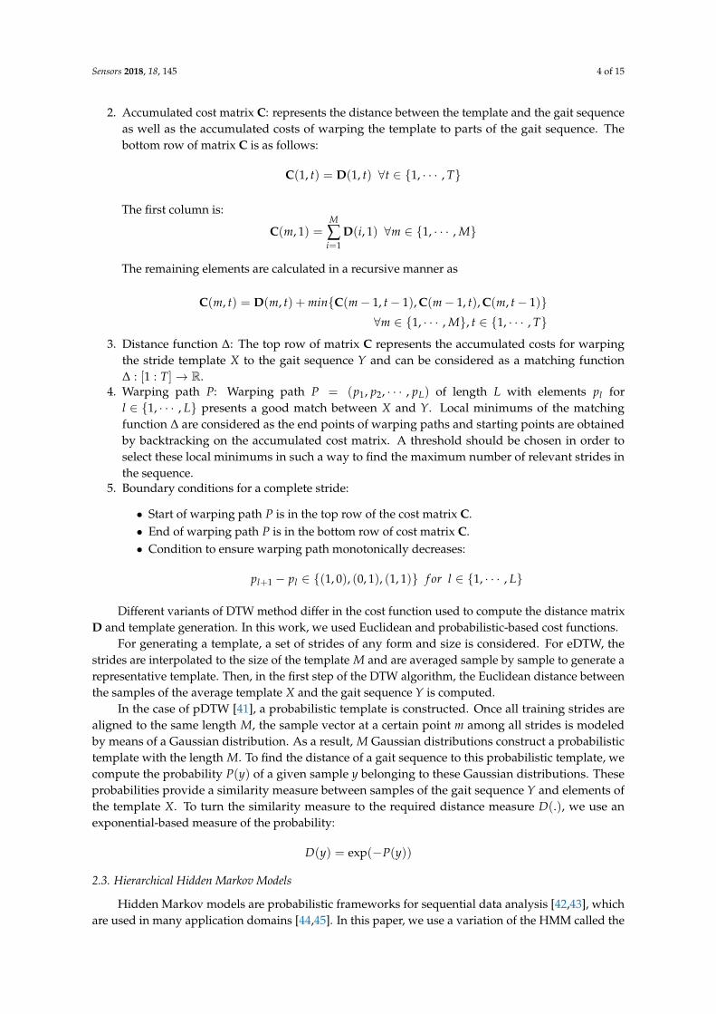
2. Accumulated cost matrix C: represents the distance between the template and the gait sequenceas well as the accumulated costs of warping the template to parts of the gait sequence. Thebottom row of matrix C is as follows:

C(1, t) = D(1, t) ∀t ∈ {1, · · · , T}

The first column is:

C(m, 1) =M

∑i=1

D(i, 1) ∀m ∈ {1, · · · , M}

The remaining elements are calculated in a recursive manner as

C(m, t) = D(m, t) + min{C(m− 1, t− 1), C(m− 1, t), C(m, t− 1)}∀m ∈ {1, · · · , M}, t ∈ {1, · · · , T}

3. Distance function ∆: The top row of matrix C represents the accumulated costs for warpingthe stride template X to the gait sequence Y and can be considered as a matching function∆ : [1 : T]→ R.

4. Warping path P: Warping path P = (p1, p2, · · · , pL) of length L with elements pl forl ∈ {1, · · · , L} presents a good match between X and Y. Local minimums of the matchingfunction ∆ are considered as the end points of warping paths and starting points are obtainedby backtracking on the accumulated cost matrix. A threshold should be chosen in order toselect these local minimums in such a way to find the maximum number of relevant strides inthe sequence.

5. Boundary conditions for a complete stride:

• Start of warping path P is in the top row of the cost matrix C.• End of warping path P is in the bottom row of cost matrix C.• Condition to ensure warping path monotonically decreases:

pl+1 − pl ∈ {(1, 0), (0, 1), (1, 1)} f or l ∈ {1, · · · , L}

Different variants of DTW method differ in the cost function used to compute the distance matrixD and template generation. In this work, we used Euclidean and probabilistic-based cost functions.

For generating a template, a set of strides of any form and size is considered. For eDTW, thestrides are interpolated to the size of the template M and are averaged sample by sample to generate arepresentative template. Then, in the first step of the DTW algorithm, the Euclidean distance betweenthe samples of the average template X and the gait sequence Y is computed.

In the case of pDTW [41], a probabilistic template is constructed. Once all training strides arealigned to the same length M, the sample vector at a certain point m among all strides is modeledby means of a Gaussian distribution. As a result, M Gaussian distributions construct a probabilistictemplate with the length M. To find the distance of a gait sequence to this probabilistic template, wecompute the probability P(y) of a given sample y belonging to these Gaussian distributions. Theseprobabilities provide a similarity measure between samples of the gait sequence Y and elements ofthe template X. To turn the similarity measure to the required distance measure D(.), we use anexponential-based measure of the probability:

D(y) = exp(−P(y))

2.3. Hierarchical Hidden Markov Models

Hidden Markov models are probabilistic frameworks for sequential data analysis [42,43], whichare used in many application domains [44,45]. In this paper, we use a variation of the HMM called the

Sensors 2018, 18, 145 5 of 15

hierarchical HMM (hHMM) [46], which is different from conventional HMMs mainly in the structureof the model. In the hHMM, it is possible to define a hierarchy of model states, which makes it moresuitable for gait segmentation.

With the standard HMM, a sequence of observations is represented using probabilisticdistributions. In this application, observations are gait data. Let us denote the observation at time tby the variable yt. We assume the observation at time t is generated by some process whose statesst are hidden. The states of this hidden process satisfy the Markov property, which means given thevalue of hidden state st−1 the current state st is independent of all the states prior to t− 1. To define aprobability distribution over observations, we need the initial probability over hidden states P(s1), thestate transition matrix defining P(st|st−1), and the observation model defining P(yt|st). In this work,observations are modeled by Gaussian mixture models (GMMs).

From a topological point of view, hHMMs [46] generalize the HMMs by making each of thehidden states a probabilistic model on its own. That is, each state is an HMM in the case of a two-levelhierarchy (see Figure 1). The HMMs in the second level have states in turn that are referred to assub-states. Transitions can be taken place between states in one level or between states and sub-statesin different levels. The lowest level sub-states define the observation model P(yt|st).

2

1 3

2

1

3

4

1

Figure 1. Topology of a two-level hierarchical hidden Markov model (hHMM). Large circles representstates in the first level of the model. Each state in turn is an HMM with sub-states (dark circles). Here,we applied left-to-right HMMs in the second level.

Learning in hHMM entails estimation of the parameters of the hHMM, including transition andinitial probabilities and GMM parameters based on given data. After learning a model, we can performinference, which in our application means finding the most probable sequence of states S∗ given anobservation sequence with the size T:

S∗ = argmaxS1:T

P(S1:T |Y1:T) (1)

3. Evaluation Study

We apply four methods, namely peak detection, eDTW, pDTW, and hHMM to the problem of gaitsegmentation from foot-worn IMUs. Peak detection, msDTW, and hHMM are widely used for gaitsegmentation. pDTW has been used in other applications such as gesture recognition [41]. To the bestof our knowledge, pDTW has not been applied to gait segmentation before. It is worth mentioning thatwhile the implementation procedures presented here can be replicated for similar cases, the examinedrange of parameters that will be presented in this section highly depends on the data set at hand.

3.1. Data Collection and Setup

Ten patients diagnosed with idiopathic PD (63 ± 9.3 years old, 5 males) with a UPDRS motorscore of 12.7 ± 6.0 and Hoehn and Yahr (H&Y) score of 1.7 ± 0.9 were included in the first experiment.For this experiment, patients walked 10 m four times at a self-selected speed. Between each 10-m walk,

Sensors 2018, 18, 145 6 of 15

there was a 180◦ turn, which was excluded from the data using videos. Hence, the final data includedonly a sequence of straight walk strides. For this experiment, the total number of strides for all patientswas 496.

For the second experiment, the population consisted of 34 patients with idiopathic PD (63 ± 11years old, 24 males). Subjects were in early to moderate stages of the disease with a UPDRS motorscore of 18.8 ± 8.9 and H&Y score of 2.2 ± 0.6. The total number of strides for this experiment was 458.Each patient performed a TUG test at a self-selected speed. The TUG test is a commonly used clinicaltest to evaluate balance and mobility. The patient stands up from a chair, walks for 3 m, performs a180◦ turn, walks back for 3 m and finally sits again [4]. The test includes straight walking and turning.In PD, turning is more impaired than straight walk [47], and hence, data from this experiment havea higher intra-patient gait variability and result in a more heterogeneous set of strides than the firstexperiment. Transitions between sit-to-stand and stand-to-sit make stride segmentation challenging,because it is essential for the methods to distinguish transition movements from stride movements. Allpatients were capable of finishing the TUG test without episodes of freezing or dyskinesia. For bothexperiments, patients gave written informed consent approved by the local committee of the medicalfaculty at University of Erlangen, Germany (Re.-No. 4208), which follows the declaration of Helsinki1975, as revised in 2000.

For both experiments, data was recorded by a Shimmer 2R (Shimmer Sensing, Dublin, Ireland)IMU, recording acceleration and angular velocity at 102.4 Hz. Each unit consisted of a tri-axialaccelerometer (range ± 6 g) and a tri-axial gyroscope (range ± 500 ◦/s). The sensor units weremounted laterally to the ankle of the patient’s right and left shoes. The measurements from both feetwere included in the experiments. Figure 2 shows the sensor placement on the shoe and the axesdefinition as well as sample data for one stride normalized to the range of the sensors (norm).

0 0.2 0.4 0.6 0.8 1

Accele

ratio

n [

no

rm]

-1

-0.5

0

0.5

1

AX AY AZ

Time[s]0 0.2 0.4 0.6 0.8 1An

gu

lar

Ve

locity [

no

rm]

-1

-0.5

0

0.5

1

GX GY GZ

Figure 2. (Left) Shimmer sensor placement and axes definition (AX, AY and AZ form three dimensionsof accelerometer and GX, GY and GZ form three dimensions of gyroscope); (Right) Accelerometer andgyroscope data for one exemplary stride.

3.2. Manual Data Labeling

The strides were labeled using simultaneous analysis of video and sensor data. The video andsensors were synchronized using a synchronization movement based on lifting one foot three times.The start and end point of each stride was labeled manually using acquired information of gyroscopeand the stride definition from [33]. Angular velocity in the sagittal plane (GZ) was used. The negativepeaks in GZ represent the change in foot rotation during one stride and were used to define start andend of the strides. Stride start was set to the negative peak before swing phase and stride end to thenegative peak at the end of the stance phase (see Figure 3). Videos were used to accurately identifythe negative peaks. In order to map each video frame to a sample in the GZ signal, a toolbox wasused, which was implemented for this purpose. The end of one stride coincides with the start of thefollowing stride for consecutive strides.

Sensors 2018, 18, 145 7 of 15

For the TUG segmentation, in addition to strides, rests and transitions were labeled. The restphase refers to the part where patient stands still and transition is any movement other than stridemovements as defined by [38]. Figure 3 shows an example of the way the gait sequence was labeled.The labeling was performed by a person familiar with gait data.

Figure 3. Labeling of an example of gyroscope signal including two strides, the following transition(non-stride) movement, and rest.

3.3. Implementation of Peak Detection

For peak detection the gyroscope signal Z-axis (GZ) (See Figure 2) was used [15,33]. Peaks in theGZ signal corresponded to the middle of swing phase in the strides. For this method, only one pointin the stride and no stride borders were recognized. There were two conditions in order to detect apeak. Firstly, angular velocity must be greater than 150 ◦/s [15,33]. Moreover, the time to previous andfollowing peaks must be greater than 600 ms, which was considered as the lower bound for length ofa stride. This time constraint was applied equally for all methods. In the case of detecting multiplepeaks in this region, only the highest amplitude was selected. For implementation, the peak detectionfunction in MATLAB 2015a was used.

3.4. Implementation of Euclidean DTW

The input to the DTW was raw data [33,38]. For template generation, we chose a template of thesize 200 samples (M = 200). Template must have a proper length to capture subtle variations in strides.Manually segmented strides were linearly interpolated to the size of 200 samples and the average of asample vector at a certain point m among all strides was computed. The template signals were thennormalized to the range of sensors (±6 g for accelerometer and ±500 ◦/s for gyroscope axes).

Figure 4 shows the signals of the template for eDTW. The signals AZ, GX, and GY are nearlyconstant and do not convey information. Hence, three signals of AZ, GX, and GY (See Figure 2) wereomitted from computations. The combination of signals and threshold used for template matchingis shown in Table 1. As mentioned in Section 2.2, thresholds in the DTW algorithm were usedto determine the end boundary of the strides, which was in turn based on the distance betweenthe template and part of the gait sequence. Using multiple axes instead of one axis increased thedistance, and therefore, the threshold was increased accordingly (see Table 1). In addition, the timeof an overlap of a given warping path must be less than 200 ms for the stride to be segmented [33].In a post-processing step, time constraints were applied to the output of the algorithm. A stride mustbe larger than 600 and smaller than 2500 ms [33]. These time constraints were equally applied forpDTW and hHHM algorithms. Template generation and eDTW algorithms were implemented inMATLAB 2015a.

Sensors 2018, 18, 145 8 of 15

Length [samples]0 40 80 120 160 200

Acce

lera

tio

n [

no

rm]

-1

-0.5

0

0.5

1

AX AY AZ

Length [samples]0 40 80 120 160 200

An

gu

lar

Ve

locity [

no

rm]

-1

-0.5

0

0.5

1

GX GY GZ

Figure 4. Template based on average of (Left) a three-dimensional accelerometer signal, (Right) athree-dimensional gyroscope signal. Signals AX, GX, and GY have a very low variation.

Table 1. Euclidean dynamic time warping (eDTW) parameters.

Signal Combination GZ AXGZ AYGZ AXAYGZ

Threshold (steps of 5) 10–25 20–30 20–30 25–40

3.5. Implementation of Probabilistic DTW

The input to pDTW is raw data and the same constraints as used in eDTW were applied here aswell. The template generation and computing distance between the gait sequence and template areexplained in Section 2.2.

The output of a probability density function is between 0 and 1 for univariate and multivariatedata. Hence, the output of the distance function is the same for single-axis (univariate) or multi-axes(multivariate) data. Accordingly, the threshold stayed the same for any combination of axes. Due tothe difference between Euclidean and probabilistic cost functions, range of thresholds for eDTW andpDTW algorithms are different. Table 2 shows the combination of the axes and thresholds. Again,template generation and pDTW algorithms were implemented in MATLAB 2015a.

Table 2. Probabilistic DTW (pDTW) parameters.

Signal Combination GZ AXGZ AYGZ AXAYGZ

Threshold (steps of 1) 8–15 8–15 8–15 8–15

3.6. Implementation of hHMM

A two-level hHMM was considered for gait segmentation for both experiments. In the firstexperiment, there was only one state to capture strides, while in the second experiment, there werethree states of stride, rest, and transition. The second level of hHMM included left-to-right HMMs,which could include multiple sub-states in turn. The exact number of sub-states was determined byoptimization. It is expected that the number of required sub-states grows as the pattern becomes morecomplex. In the first level, learning was done in a supervised manner using labels of stride borders,while in the second level, an unsupervised approach was applied. The advantage of semi-supervisedlearning is that we do not need to provide labels for the second level, but learning is done based on theunderlying data.

The input to the hHMM was a set of features extracted from the raw data using the sliding windowapproach. In this approach, the data was segmented into overlapping time frames. The windowingwas done using the Hann window instead of rectangular window in order to reduce the effect ofwindowing on the edges. From each window a set of features was extracted, including the raw dataitself, mean, variance, energy and three coefficient of the second order polynomial fit [38]. The finalfeature set was constructed by concatenating the features from all IMU axes. The feature set was thennormalized. The size of the sliding window was chosen in a way that the features best represent the

Sensors 2018, 18, 145 9 of 15

underlying data. Several window sizes were tried as in [36,38]. To get the most relevant features andreduce the dimensionality of data (and therefore number of parameters), we used principal componentanalysis (PCA).

For optimizing the number of principal components that was fed to the hHMM, as well asparameters that controlled the structure of the hHMM (such as number of sub-states and numberof components per GMM), a grid search was used. Table 3 shows the values for these parameters,which were chosen partially based on literature [36,38] and partially empirically. hHMM modelparameters included transition matrices and initial state probabilities as well as GMM parameters,including means, diagonal covariance matrices, and weights of GMM components. The first-leveltransition matrix and GMM parameters were initialized based on the data distribution. Transitionmatrices for second-level HMMs were initialized uniformly. For learning model parameters, theBaum–Welch (BW) [48] algorithm was applied, which is a special case of the expectation maximization(EM) algorithm [49]. The BW algorithm was performed at most for 20 iterations. For inference and gaitsegmentation the Viterbi algorithm [50] was used.

For feature extraction and dimensionality reduction, MATLAB 2015a was used because it providedall the necessary functions. For learning and inference of the hHMM the Java Speech Toolkit (JSTK)was used [51], since this toolbox allows for semi-supervised learning and inference.

Table 3. hHMM parameters.

Parameters Values

Sliding window length (s) (steps of 0.20) 0.10–0.70

Number of sub-states for stride | transition | rest (steps of 2) 4–12 | 2–4 | 1

Number of Gaussian mixture model (GMM) components (steps of 2) 8–12

Number of principal components (steps of 2) 1–15

3.7. Performance Assessment

The goal in segmentation was two-fold: (1) to minimize the number of missed strides; and (2) tominimize signal parts which are wrongly detected as strides. True positives (TPs) are strides segmentedby the method and are also labeled as strides in the ground truth. False negatives (FNs) are the stridesthat are not recognized by the segmentation algorithms. If there is no ground truth stride and a methodsegments a stride, for example, at rest or in transition time, then a false positive (FP) occurs. Basedon the mentioned parameters, three metrics are computed. Precision considers false positives and isequal to one only if all the recognized strides are labeled in the ground truth. Recall considers the falsenegatives and is equal to one if no stride is missed. The F-score, which takes into account missingstrides and wrongly detected strides equally, is the main metric for comparison of methods and gridsearch optimization has been performed based on that.

Precision =ΣTP

ΣTP + ΣFP(2)

Recall =ΣTP

ΣTP + ΣFN(3)

F-score = 2× Precision× RecallPrecision + Recall

(4)

For all methods the segmented strides were compared with the ground truth stride borders andwere marked as correctly segmented if the start and end borders were within ±100 ms of the groundtruth borders, which is approximately 10% of stride time [33,37,52].

Sensors 2018, 18, 145 10 of 15

4. Experimental Results

The first experiment was performed in a leave-one-out cross validation scheme. Data from bothfeet of one patient were left out on each iteration and the rest of the data was used as a training set.Parameter tuning as well as template generation were performed based on the training set. Three ofthe methods of choice (hHMM, eDTW and peak detection) could detect all strides with a F-score of100%. Probabilistic DTW yielded a slightly worse result, with the F-score of 99.8 ± 0.4%.

In the case of the second experiment, due to the larger data set, a 4-fold outer cross-validationwas applied for the evaluation of methods. For validation and parameter estimation, an inner 4-foldcross validation was used. The cross-validation was performed such that no patient used for trainingand validation appeared in the test set. To remove any possible bias, the data was randomized forchoosing the test and validation sets. The randomization was equally applied for all methods. Table 4lists average statistics across test folds for the best set of parameters in each method. Methods wereevaluated based on their F-scores.

Table 4. Results of the second experiment in terms of precision, recall, and F-score.

Method Precision (%) Recall (%) F-score (%)

hHMM 98.5 ± 0.4 93.5 ± 1.9 95.9 ± 0.9

eDTW 94 ± 1.2 93.5 ± 0.8 93.8 ± 0.5

Peak detection 87.4 ± 1.2 95.9 ± 1.8 91.5 ± 0.4

pDTW 91.8 ± 2.1 90.1 ± 2.2 90.9 ± 1.4

To identify significant differences between methods, statistical tests were performed. TheWilcoxon test was used as a non-parametric statistical test for pair-wise comparison of the resultbecause of the small number of samples and possibility of having non-normal distributions. Figure 5shows the result of the pair-wise tests. In the case of precision, all tests showed a significant difference(p < 0.05) except for the comparison of eDTW to pDTW (p = 0.20). The result showed higher variancefor the recall metric. The methods showed no significant difference (p > 0.05) in the case of recallexcluding the test between peak detection and pDTW (p < 0.05). For the F-scores, the variance for allmethods decreased, which accounted for the significant difference in most of the tests (p < 0.05) exceptfor the test between peak detection and pDTW (p = 0.88).

* * **

*

Precision

hHM

M

eDTW

Peak Det

ectio

n

pDTW

0

20

40

60

80

100*

Recall

hHM

M

eDTW

Peak Det

ectio

n

pDTW

0

20

40

60

80

100* *

**

*F-score

hHM

M

eDTW

Peak Det

ectio

n

pDTW

0

20

40

60

80

100

Figure 5. Mean ± STD of precision, recall and F-score for four methods. Asterisks represent a 5%significant difference between methods corresponding to 95% confidence interval.

5. Discussion and Conclusion

One main approach to the quantitative assessment of gait in PD is to analyze spatio-temporalparameters extracted from individual gait strides [53,54], which highlights the importance of robuststride segmentation. We compared four prominent segmentation methods with the focus on

Sensors 2018, 18, 145 11 of 15

pathological gait of PD patients. In order to cover wide range of gait studies in PD [15,39,40], weassessed gait segmentation methods under two scenarios with different levels of complexity. In thefirst scenario, a data set including only straight walk was considered. The second scenario focused on amore challenging data set including stride and non-stride movements, as well as turnings. Intra-patientgait variability increased as turning strides were combined with strides from straight walking.

The result from the first scenario showed the methods perform similarly well, with 100% accuracy.This result suggested that when there is only a sequence of strides with low variability derived froma very rigid supervised test assessment paradigm, all methods perform similarly. In such cases, onemay consider using a simpler and faster method, especially for large data sets. The peak detectionmethod does not need parameter learning and is the fastest method. On the other hand, there areHMM methods for which the parameter learning phase can be computationally costly. However, oncethe model is learned, it can be used for further gait segmentation either in an offline or online mode.

In contrast, in the second scenario, the performance of all methods diminished considerably.The methods also demonstrated different performances (see Table 4). The hHMM significantlyoutperformed the other methods with an accuracy of 96% and a low standard deviation, whichis a promising result for gait analysis applications. eDTW yielded a 94% F-score while peak detectionand pDTW obtained only a 91% and 90% F-score, respectively.

Gait analysis systems using wearable inertial sensors have made long-term monitoring of PDpatients possible. Different studies were conducted to monitor and analyze gait fluctuations inPD during the course of a day [55,56]. The most important aspect of a gait segmentation methodfor long-term monitoring lies in its ability to deal with gait variability in a non-supervised andnon-standardized test setting with a high accuracy. Our experiments demonstrate how the methodscan deal with variability, though on a smaller scale than in long-term monitoring.

The power of ML methods is increasingly appreciated in PD studies [18,40]. They also provepromising in the case of sensor-based gait segmentation [35,38]. Our results revealed that for dealingwith inter- and intra-patient gait variability, hHMM methods surpassed the other methods. The hHMMachieved a high precision of nearly 99%, meaning that there was a low rate of false positives. Theprobabilistic representation of the data was effective in distinguishing between stride and non-stridemovements and there were only a few cases in which non-stride movements were segmented asstrides. The other group of ML methods that can be used for stride segmentation are deep learning(DL) methods [18,57], which in the emergence of high computational power and large data sets becomeincreasingly popular. DL methods have advantages over HMM methods, since they perform featureextraction automatically. However, learning their large parameter space requires availability of a largedata set. Size of our data set ruled out the possibility of applying these methods.

eDTW significantly surpassed pDTW by 4% in terms of the F-score. The templates in eDTWwere generated simply by computing the average of strides, while in pDTW a series of probabilitydistributions modeled the template. It was speculated that a probabilistic template would result in amore flexible template than an average-based template. However, in practice, eDTW proved moreeffective in gait segmentation. It is worth noting that pDTW is a probabilistic template matchingmethod and does not utilize the fully probabilistic representation of data the same way as HMMmethods do.

Peak detection yielded the best recall of 95% among all methods in the second experiment. Froma methodological point of view, peak detection is a very simple method in which, unlike hHHM andDTW methods, there is no need for parameter learning. In particular, peak detection is a good methodof choice in case of small size data sets, where enough data is not available for parameter tuning.However, the low precision rate in the case of the second experiment suggests that the applicability ofthis method is limited in case of more complicated data sets, since it produces many false positives.

Although the F-score was the main metric for performance evaluation, in clinical applicationsof gait analysis, a low false positive rate is more critical than a low false negative rate. This isbecause clinical gait analysis, which follows gait segmentation, is based on statistics of spatio-temporal

Sensors 2018, 18, 145 12 of 15

parameters extracted from strides. Parameters extracted from false positive strides may destroy theunderlying statistics. Hence, in PD studies the precision is more critical than the recall. Precisionversus recall tendencies vary among methods. DTW methods showed a balance between precisionand recall, while hHMM yielded a high precision and peak detection a high recall. Precision in hHMMis significantly higher than all other methods.

The main limitation of the methods stemmed from their low recall rate. Statistical analysis showedno significant difference between recall rates, except for the comparison between pDTW and peakdetection. The methods segmented all strides correctly in a homogeneous sequence as shown bythe first experiment. However, in a heterogeneous setting, (as shown by our second experiment), allmethods tended to miss strides that deviate from normal strides in form and length. In such cases,hHMM might fail to generalize to these strides and the template in DTW methods might not be able tomatch such strides. One solution for that is to have a large enough number of such atypical stridesin the data set. Although we used one of the largest data sets for the gait segmentation problem inthe literature [34,38], an even larger population may mitigate the problem of variable strides. It is ageneral rule in any application that a large population can lead to a better representation of data inHMM and in the same manner more generic templates for DTW methods.

The inter-patient gait variability may be more effectively addressed using individualized models,in such a way that models better reflect the specific gait charactristics of each individual patient. Inparticular, as the PD progresses, the motor impairment deteriorates, which results in a larger deviationof pathological gait from normal gait. An atypical gait pattern that largely deviates from the average ofthe population results in a poor performance of the methods. In such extreme cases individualizationcan be helpful. hHMM provides the theoretical foundation to adapt models to individual patients [58].For DTW methods, it is also possible to construct templates based on an individual patient. Anindividualized template may map the patient’s strides better than a generic template.

Lastly, gait analysis can provide valuable clinical information also for other neurological disordersthat affect gait such as HSP [38] or multiple sclerosis. Gait disturbances vary among these diseases,and hence, segmentation methods should be adapted to specific gait patterns of each disease.

In summary, automated mobile gait analysis offers an elaborate assessment of pathologicalgait, leading to a deeper insight into PD. To assess sensor-based gait segmentation, which is animportant building block in the process of gait analysis, we compared four segmentation methodswidely used in the literature. The experiments showed the accuracy of segmentation methods to agreat extent depends on the stride variability in data sets that is mainly derived from the variationsof the instrumented test paradigm, the pathological gait of PD patients, the specific gait patternsof each patient, and the difference between straight and turning movements. In the case of ahomogeneous data, even a simple method such as peak detection proved effective, while, in thecase of more heterogeneous assessment paradigms reflecting the standardized test paradigms alongwith non-supervised and non-standardized assessments e.g. in long-term monitoring, probabilistichHMM significantly outperformed the other methods. The results of the current study can be appliedto any PD studies inside the clinic and provide useful insights for long-term monitoring outsidethe clinic.

Acknowledgments: The authors would like to thank J. Barth, S. Reinfelder, and K. Weinmann for assistance withdata collection, as well as study participants. N. Haji Ghassemi acknowledges financial support from the BavarianResearch Foundation (BFS). This work was in part supported by the FAU Emerging Fields Initiative (EFIMoves).Björn M. Eskofier gratefully acknowledges the support of the German Research Foundation (DFG) within theframework of the Heisenberg professorship program (grant number ES 434/8-1).

Author Contributions: N.H., M.M., J.K. and B.M.E. conceived and designed the experiments; N.H., J.H. andC.F.M. performed the experiments; N.H., J.H., H.G., M.M., J.K. and B.M.E. analysed the data; N.H. wrote thepaper. All authors critically reviewed the manuscript and approved the final version.

Conflicts of Interest: The authors declare no conflict of interest. The founding sponsors had no role in the designof the study; in the collection, analyses, or interpretation of data; in the writing of the manuscript, and in thedecision to publish the results.

Sensors 2018, 18, 145 13 of 15

1. Parkinson, J. An Essay on the Shaking Palsy; Neely & Jones: London, UK, 1817.2. Hoehn, M.M.; Yahr, M.D. Parkinsonism: Onset, progression and mortality. Neurology 1967, 17, 427–442.3. Goetz, C.G.; Tilley, B.C.; Shaftman, S.R.; Stebbins, G.T.; Fahn, S.; Martinez-Martin, P.; Poewe, W.;

Sampaio, C.; Stern, M.B.; Dodel, R.; et al. Movement Disorder Society-sponsored revision of the UnifiedParkinson’s Disease Rating Scale (MDS-UPDRS): Scale presentation and clinimetric testing results.Movement Disord. 2008, 23, 2129–2170.

4. Podsiadlo, D.; Richardson, S. The timed "Up & Go": A test of basic functional mobility for frail elderlypersons. J. Am. Geriatr. Soc. 1991, 39, 142–148.

5. Marchese, R.; Bove, M.; Abbruzzese, G. Effect of cognitive and motor tasks on postural stability inParkinson’s disease: A posturographic study. Movement Disord. 2003, 18, 652–658.

6. Richards, M.; Marder, K.; Cote, L.; Mayeux, R. Interrater reliability of the unified Parkinson’s disease ratingscale motor examination. Movement Disord. Jan 1994, 9, 89–91.

7. Maetzler, W.; Klucken, J.; Horne, M. A clinical view on the development of technology-based tools inmanaging Parkinson’s disease. Movement Disord. 2016, 31, 1263–1271.

8. Klucken, J.; Friedl, K.; Eskofier, B.M.; Hausdorf, J.M. Guest Editorial: Enabling Technologies for Parkinson’sDisease Management. IEEE J. Biomed. Health Inform. 2015, 19, 1775–1776.

9. Espay, A.J.; Bonato, P.; Nahab, F.B.; Maetzler, W.; Dean, J.M.; Klucken, J.; Eskofier, B.M.; Merola, A.;Horak, F.; Lang, A.E.; et al. Technology in Parkinson’s disease: Challenges and opportunities.Movement Disord. 2016, 31, 1272–1282.

10. Gray, P.; Hildebrand, K. Fall risk factors in Parkinson’s disease. J. Neurosci. Nurs. 2000, 32, 222–228.11. Schrag, A.; Jahanshahi, M.; Quinn, N. How does Parkinson’s disease affect quality of life? A comparison

with quality of life in the general population. Movement Disord. 2000, 15, 1112–1118.12. Salarian, A.; Russmann, H.; Vingerhoets, F.J.; Dehollain, C.; Blanc, Y.; Burkhard, P.R.; Aminian, K.

Gait assessment in Parkinson’s disease: Toward an ambulatory system for long-term monitoring.IEEE Trans. Biomed. Eng. 2004, 51, 1434–1443.

13. Chen, B.R.; Patel, S.; Buckley, T.; Rednic, R.; McClure, D.J.; Shih, L.; Tarsy, D.; Welsh, M.; Bonato, P.A web-based system for home monitoring of patients with Parkinson’s disease using wearable sensors.IEEE Trans. Biomed. Eng. 2011, 58, 831–836.

14. Kluge, F.; Gaßner, H.; Hannink, J.; Pasluosta, C.; Klucken, J.; Eskofier, B.M. Towards Mobile Gait Analysis:Concurrent Validity and Test-Retest Reliability of an Inertial Measurement System for the Assessment ofSpatio-Temporal Gait Parameters. Sensors 2017, 17, 1522.

15. Mariani, B.; Jiménez, M.C.; Vingerhoets, F.J.; Aminian, K. On-shoe wearable sensors for gait and turningassessment of patients with Parkinson’s disease. IEEE Trans. Biomed. Eng. 2013, 60, 155–158.

16. Pasluosta, C.F.; Gassner, H.; Winkler, J.; Klucken, J.; Eskofier, B.M. An emerging era in the management ofParkinson’s disease: Wearable technologies and the internet of things. IEEE J. Biomed. Health Inf. 2015,19, 1873–1881.

17. Rampp, A.; Barth, J.; Schülein, S.; Gaßmann, K.G.; Klucken, J.; Eskofier, B.M. Inertial Sensor-BasedStride Parameter Calculation From Gait Sequences in Geriatric Patients. IEEE Trans. Biomed. Eng. 2015,62, 1089–1097.

18. Hannink, J.; Kautz, T.; Pasluosta, C.; Barth, J.; Schulein, S.; Gassmann, K.G.; Klucken, J.; Eskofier, B. MobileStride Length Estimation with Deep Convolutional Neural Networks. IEEE J. Biomed. Health Inf. 2017.

19. Trojaniello, D.; Cereatti, A.; Pelosin, E.; Avanzino, L.; Mirelman, A.; Hausdorff, J.M.; Della Croce, U.Estimation of step-by-step spatio-temporal parameters of normal and impaired gait using shank-mountedmagneto-inertial sensors: Application to elderly, hemiparetic, parkinsonian and choreic gait. J. Neuroeng. Rehabil.2014, 11, 152.

20. Kang, H.G.; Dingwell, J.B. Separating the effects of age and walking speed on gait variability. Gait Posture2008, 27, 572–577.

21. Kluge, F.; Krinner, S.; Lochmann, M.; Eskofier, B.M. Speed dependent effects of laterally wedged insoles ongait biomechanics in healthy subjects. Gait Posture 2017, 55, 145–149.

22. Agostini, V.; Balestra, G.; Knaflitz, M. Segmentation and classification of gait cycles. IEEE Trans. Neur. Syst.Rehabil. Eng. 2014, 22, 946–952.

Sensors 2018, 18, 145 14 of 15

23. Agostini, V.; Gastaldi, L.; Rosso, V.; Knaflitz, M.; Tadano, S. A Wearable Magneto-Inertial System for GaitAnalysis (H-Gait): Validation on Normal Weight and Overweight/Obese Young Healthy Adults. Sensors2017, 17, 2406.

24. Selles, R.W.; Formanoy, M.A.G.; Bussmann, J.B.J.; Janssens, P.J.; Stam, H.J. Automated Estimation of Initialand Terminal Contact Timing Using Accelerometers; Development and Validation in Transtibial Amputeesand Controls. IEEE Trans. Neur. Syst. Rehabil. Eng. 2005, 13, 81–88.

25. Derawi, M.O.; Bours, P.; Holien, K. Improved Cycle Detection for Accelerometer Based Gait Authentication.In Proceedings of the Sixth International Conference on Intelligent Information Hiding and MultimediaSignal Processing, Darmstadt, Germany, 15–17 October 2010.

26. Libby, R. A simple method for reliable footstep detection on embedded sensor platforms. 2008.Available Online: https://www.researchgate.net/publication/265189201_A_simple_method_for_reliable_footstep_detection_on_embedded_sensor_platforms. (accessed on 6 January 2018).

27. Hundza, S.R.; Hook, W.R.; Harris, C.R.; Mahajan, S.V.; Leslie, P.A.; Spani, C.A.; Spalteholz, L.G.; Birch, B.J.;Commandeur, D.T.; Livingston, N.J. Accurate and reliable gait cycle detection in Parkinson’s disease.IEEE Trans. Neur. Syst. Rehabil. Eng. 2014, 22, 127–137.

28. Aminian, K.; Najafi, B.; Büla, C.; Leyvraz, P.F.; Robert, P. Spatio-temporal parameters of gait measured byan ambulatory system using miniature gyroscopes. J. Biomech. 2002, 35, 689–699.

29. Khandelwal, S.; Wickstrom, N. Identification of Gait Events using Expert Knowledge and ContinuousWavelet Transform Analysis. In Proceedings of the International Conference on Bio-inspired Systems andSignal Processing, Angers, France, 3–6 March 2014; pp. 197–204.

30. Gouwanda, D.; Senanayake, S.A. Application of hybrid multi-resolution wavelet decomposition methodin detecting human walking gait events. In Proceedings of the International Conference of Soft Computingand Pattern Recognition, Malacca, Malaysia, 4–7 December 2009; pp. 580–585.

31. Müller, M. Dynamic time warping. In Information Retrieval for Music and Motion; Springer: New York, NY,USA, 2007; pp. 69–84.

32. ten Holt, G.A.; Reinders, M.J.; Hendriks, E.A. Multi-Dimensional Dynamic Time Warping for GestureRecognition. In Proceedings of the Thirteenth annual conference of the Advanced School for Computingand Imaging, Heijen, The Netherlands, 13–15 June 2007.

33. Barth, J.; Oberndorfer, C.; Pasluosta, C.; Schülein, S.; Gassner, H.; Reinfelder, S.; Kugler, P.; Schuldhaus, D.;Winkler, J.; Klucken, J.; et al. Stride segmentation during free walk movements using multi-dimensionalsubsequence dynamic time warping on inertial sensor data. Sensors 2015, 15, 6419–6440.

34. Mannini, A.; Sabatini, A.M. A hidden Markov model-based technique for gait segmentation usinga foot-mounted gyroscope. In Proceedings of the 33th Annual International Conference of the IEEEEngineering in Medicine and Biology Society (EMBC), Boston, MA, USA, 30 Auguest–3 September 2011;pp. 4369–4373.

35. Mannini, A.; Trojaniello, D.; Della Croce, U.; Sabatini, A.M. Hidden Markov model-based strategy for gaitsegmentation using inertial sensors: Application to elderly, hemiparetic patients and Huntington’s diseasepatients. In Proceedings of the 37th Annual International Conference of the IEEE Engineering in Medicineand Biology Society (EMBC), Milano, Italy, 25–29 August 2015; pp. 5179–5182.

36. Panahandeh, G.; Mohammadiha, N.; Leijon, A.; Handel, P. Continuous Hidden Markov Model forPedestrian Activity Classification and Gait Analysis. IEEE Trans. Instrum. Meas. 2013, 62, 1073–1083.

37. Pfau, T.; Ferrari, M.; Parsons, K.; Wilson, A. A hidden Markov model-based stride segmentation techniqueapplied to equine inertial sensor trunk movement data. J. Biomech. 2008, 41, 216–220.

38. Martindale, C.F.; Strauss, M.; Gaßner, H.; List, J.; Müller, M.; Klucken, J.; Kohl, Z.; Eskofier, B.M.Segmentation of Gait Sequences using Inertial Sensor Data in Hereditary Spastic Paraplegia. In Proceedingsof the International Conference of the IEEE Engineering in Medicine and Biology Society (EMBC),Jeju Island, Korea, 11–15 July 2017.

39. El-Gohary, M.; Pearson, S.; McNames, J.; Mancini, M.; Horak, F.; Mellone, S.; Chiari, L. Continuousmonitoring of turning in patients with movement disability. Sensors 2014, 14, 356–369.

40. Klucken, J.; Barth, J.; Kugler, P.; Schlachetzki, J.; Henze, T.; Marxreiter, F.; Kohl, Z.; Steidl, R.; Hornegger, J.;Eskofier, B.; Winkler, J. Unbiased and Mobile Gait Analysis Detects Motor Impairment in Parkinson’sDisease. PLoS ONE 2013, 8, doi: 10.1371/journal.pone.0056956.

Sensors 2018, 18, 145 15 of 15

41. Bautista, M.; Hernandez-Vela, A.; Ponce, V.; Perez-Sala, X.; Bar, X.; Pujol, O.; Angulo, C.; Escalera, S.Probability-based Dynamic Time Warping for Gesture Recognition on RGB-D data. Adv. Depth ImageAnal. Appl. 2013, 7854, 126–135.

42. Rabiner, L.; Juang, B. An introduction to hidden Markov models. IEEE ASSP Mag. 1986, 3, 4–16.43. Ghahramani, Z. An introduction to hidden Markov models and Bayesian networks. Int. J. Pattern Recogn.

2001, 15, 9–42.44. Gales, M.; Young, S. The application of hidden Markov models in speech recognition. In Foundations

and Trends in Signal Processing; Now Publishers Inc.: Hanover, MA, USA, 2008; Volume 1, pp. 195–304,doi:10.1561/2000000004.

45. Lukashin, A.V.; Borodovsky, M. GeneMark.hmm: New solutions for gene finding. Nucleic Acids Res. 1998,26, 1107–1115.

46. Fine, S.; Singer, Y.; Tishby, N. The hierarchical hidden Markov model: Analysis and applications.Mach. Learn. 1998, 32, 41–62.

47. Crenna, P.; Carpinella, I.; Rabuffetti, M.; Calabrese, E.; Mazzoleni, P.; Nemni, R.; Ferrarin, M. Theassociation between impaired turning and normal straight walking in Parkinson’s disease. Gait posture2007, 26, 172–178.

48. Bilmes, J.A. A Gentle Tutorial of the EM Algorithm and Its Application to Parameter Estimation for GaussianMixture and Hidden Markov Models; University of Berkeley: Berkeley, CA, USA, 1997.

49. Dempster, A.P.; Laird, N.M.; Rubin, D.B. Maximum likelihood from incomplete data via the EM algorithm.J. R. Stat. Soc. Series B Methodol 1977, 1–38.

50. Viterbi, A. Error bounds for convolutional codes and an asymptotically optimum decoding algorithm.IEEE Trans. Inf. Theory 1967, 13, 260–269.

51. Steidl, S.; Riedhammer, K.; Bocklet, T.; Florian, H.; Nöth, E. Java Visual Speech Components for RapidApplication Development of GUI based Speech Processing Applications. In Proceedings of the 12th AnnualConference of the International Speech Communication Association 2011 (INTERSPEECH 2011), Florence,Italy, 28–31 August 2011.

52. Mannini, A.; Sabatini, A.M. Gait phase detection and discrimination between walking–jogging activitiesusing hidden Markov models applied to foot motion data from a gyroscope. Gait posture 2012, 36, 657–661.

53. Schlachetzki, J.C.; Barth, J.; Marxreiter, F.; Gossler, J.; Kohl, Z.; Reinfelder, S.; Gassner, H.; Aminian, K.;Eskofier, B.M.; Winkler, J.; et al. Wearable sensors objectively measure gait parameters in Parkinson’sdisease. PLoS ONE 2017, 12, e0183989.

54. Gaßner, H.; Marxreiter, F.; Kohl, Z.; Schlachetzki, J.; Eskofier, B.; Winkler, J.; Klucken, J. Impaired gaitparameters are more sensitive for dual task performance than cognitive impairment in Parkinson’s disease.Basal Ganglia 2017, 8, 3.

55. Zampieri, C.; Salarian, A.; Carlson-Kuhta, P.; Nutt, J.G.; Horak, F.B. Assessing mobility at home in peoplewith early Parkinson’s disease using an instrumented Timed Up and Go test. Parkinsonism Relat. Disord.2011, 17, 277–280.

56. Saito, N.; Yamamoto, T.; Sugiura, Y.; Shimizu, S.; Shimizu, M. Lifecorder: A new device for the long-termmonitoring of motor activities for Parkinson’s disease. Intern. Med. 2004, 43, 685–692.

57. LeCun, Y.; Bengio, Y.; Hinton, G. Deep learning. Nature 2015, 521, 436–444.58. Leggetter, C.J.; Woodland, P.C. Maximum likelihood linear regression for speaker adaptation of continuous

density hidden Markov models. Comput. Speech Lang. 1995, 9, 171–185.

c© 2018 by the authors. Licensee MDPI, Basel, Switzerland. This article is an open accessarticle distributed under the terms and conditions of the Creative Commons Attribution(CC BY) license (http://creativecommons.org/licenses/by/4.0/).