Sediment Assessment Methods - Cawthron Institute · 4.2 Review of sediment assessment methods ......
108
Sediment Assessment Methods • Section 1. Introduction 1 Joanne Clapcott Roger Young Jon Harding Christoph Matthaei John Quinn Russell Death Sediment Assessment Methods Protocols and guidelines for assessing the effects of deposited fine sediment on in-stream values
Transcript of Sediment Assessment Methods - Cawthron Institute · 4.2 Review of sediment assessment methods ......

Sediment Assessment Methods • Section 1. Introduction 1
Joanne ClapcottRoger YoungJon HardingChristoph MatthaeiJohn QuinnRussell Death
Sediment Assessment Methods
Protocols and guidelines for assessing the effects of deposited fine sediment on in-stream values


Joanne ClapcottRoger YoungJon HardingChristoph MatthaeiJohn QuinnRussell Death
Sediment Assessment
MethodsProtocols and guidelines for assessing the effects of deposited fine sediment
on in-stream values

Sediment Assessment Methods
Protocols and guidelines for assessing the effects of deposited fine sediment on in-stream values
Published by
Cawthron InstitutePrivate Bag 2Nelson 7042New Zealandwww.cawthron.org.nz
Citation
Clapcott, J.E., Young, R.G., Harding, J.S., Matthaei, C.D., Quinn, J.M. and Death, R.G. (2011) Sediment Assessment Methods: Protocols and guidelines for assessing the effects of deposited fine sediment on in-stream values. Cawthron Institute, Nelson, New Zealand.
Copyright
© Cawthron Institute 2011. All rights reserved.
The information provided in this publication is for non-commercial reference purposes only. Whilst Cawthron Institute and the authors have used all reasonable endeavours to ensure the information contained in this publication is accurate, no expressed or implied warranty is given by Cawthron Institute (or the authors) as to the accuracy or completeness of the information. Neither Cawthron Institute nor the authors shall be liable for any claim, loss, or damage suffered or incurred in relation to, or as a result of, the use of the information contained within this publication.
ISBN: 978-0-473-20105-0 (Print) ISBN: 978-0-473-20106-7 (Online)
Cover images
Front cover - Wai-iti River (Kati Doehring); Okeover Stream (Jon Harding); Summer Warr trials the Shuffle method in the Porirua River (Juliet Milne); Kati Doehring trials the in-stream visual assessment method in the Wai-iti River (Joanne Clapcott); Ashley River (Mary Beech).Back cover – St Albans stream showing the effects of liquefaction following the Christchurch earthquake, February 2011 (Jon Harding); Shuffle method in Heriot Burn (Justin Kitto); Ashley River (Mary Beech); St Albans stream (Jon Harding); Wairau River (Karen Shearer).
Graphic design
Downing Design, Nelson, New Zealand.
Acknowledgements
We are indebted to a large group of freshwater scientists and technicians who contributed to the development of protocols and guidelines presented in this document. First and foremost, 12 regional councils field tested protocols and provided valuable feedback and data, hence we are very grateful to the following and their field teams – Katrina Hansen (Northland Regional Council), Martin Neale (Auckland Regional Council), Kevin Collier and Mark Hamer (Environment Waikato), Kimberley Hope and Chris Fowles (Taranaki Regional Council), Sandy Haidekker (Hawkes Bay Regional Council), Kate McArthur and Carol Nicholson (Horizons Regional Council), Summer Warr and Alton Perrie (Greater Wellingtin Regional Council), Fleur Tiernan (Marlborough District Council), Trevor James (Tasman District Council), Mary Beech (Environment Canterbury), Justin Kitto and Rachel Ozanne (Otago Regional Council) and Kirsten Meijer (Environment Southland). Several of these people also provided photos contained within. We also thank participants at workshops held at the Ministry for the Environment in Wellington 2009 and at the New Zealand Freshwater Sciences Society Conference in Whangarei in 2009 and in Christchurch in 2010. Adrian Meredith, Kate McArthur, Graham-Sevicke Jones, Mary Beech, Juliet Milne, and Kirsten Meijer were members of the regional council steering committee that developed the brief for the project. We thank Les Basher and Olivier Ausseil for their advice throughout. We thank Eric Goodwin for contributing to the development of the boosted regression tree model and Kati Doehring for her assistance with spatial analysis. We thank David Reid, Kati Doehring , Duncan Gray and postgraduate students of the School of Biological Sciences (University of Canterbury) for their fieldwork contribution. We thank postgraduate students at the University of Otago, NIWA laboratory staff and Environment Canterbury for processing samples. We thank Annika Wagenhoff, Javad Ramezani and Logan Brown for providing additional data for guideline development and we thank Summer Warr, Kate McArthur, Mary Beech and Oliver Ausseil for providing editorial feedback on earlier versions of this document. The Sediment Assessment Methods were funded by the Envirolink Tools programme through the Ministry for Science and Innovation. We thank the Ministry for the Environment for helping publish this document and we thank Cherie Johansson for proofreading and arranging publication.

Sediment Assessment Methods • Section 1. Introduction 5
1. Introduction .............................................................................. 7
1.1 Background .........................................................................................................................................81.2 Scope ......................................................................................................................................................91.3 Defining deposited fine sediment ........................................................................................91.4 Sediment and in-stream values ...........................................................................................10
2. Sediment protocols ................................................................ 11
2.1 Guiding principles ........................................................................................................................122.1.1 Site selection ........................................................................................................................122.1.2 Sample collection .............................................................................................................12
2.2 Method selection and field validation ............................................................................132.3 Recommended protocols .......................................................................................................14
SAM 1 - Bankside visual estimate of sediment ..........................................................15SAM 2 – In-stream visual assessment of sediment .................................................17SAM 3 – Wolman pebble count ..........................................................................................21SAM 4 – Resuspendable sediment (Quorer method) ...........................................23SAM 5 – Resuspendable sediment (Shuffle index) .................................................25SAM 6 – Sediment depth ........................................................................................................27
3. Sediment guidelines .............................................................. 29
3.1 Guiding principles ........................................................................................................................303.1.1 Values-based assessment .............................................................................................303.1.2 Hard- versus soft-bottomed streams ....................................................................303.1.3 Accounting for temporal and spatial variability .............................................31
3.2 Determining sediment guideline values .......................................................................313.3 Recommended guidelines .....................................................................................................33
4. Supporting information ......................................................... 37
4.1 Review of sediment effects on biota and in-stream values ...............................384.1.1 Benthic invertebrates ......................................................................................................384.1.2 Fish..............................................................................................................................................444.1.3 Recreational and aesthetic values ..........................................................................46
4.2 Review of sediment assessment methods ...................................................................474.2.1 Percent cover of sediment ..........................................................................................484.2.2 Particle size distribution ................................................................................................504.2.3 Relative bed stability .......................................................................................................514.2.4 Embeddedness ...................................................................................................................524.2.5 Suspendible fines ..............................................................................................................524.2.6 Sediment depth .................................................................................................................544.2.7 Volume of fines in pools ................................................................................................55
Contents

Sediment Assessment Methods • Section 1. Introduction6
4.3 Protocol testing and validation ............................................................................................554.3.1 Do results vary for different habitats? ...................................................................564.3.2 Do results vary among different users? ...............................................................574.3.3 Do results vary in different land uses? ..................................................................594.3.4 How do results vary over time? ................................................................................604.3.5 How many replicates are required? .......................................................................624.3.6 How do results from different protocols compare? ....................................634.3.7 Are there cheaper, quicker methods? ..................................................................644.3.8 How well are sediment metrics related to in-stream biota? ..................664.3.9 Other useful things discovered along the way ..............................................67
4.4 Review of existing guidelines ...............................................................................................704.4.1 New Zealand ........................................................................................................................704.4.2 International .........................................................................................................................70
4.5 Guideline development ...........................................................................................................704.5.1 Sources of data ...................................................................................................................724.5.2 Correlation among sediment and biota .............................................................734.5.3 Predictive relationships between sediment and biota ..............................754.5.4 Boosted regression tree model to inform reference state .......................774.5.5 Data mining to inform reference state ................................................................824.5.6 Amenity values ...................................................................................................................844.5.7 Fish values ..............................................................................................................................88
5. References ............................................................................... 89
6. Appendices ............................................................................. 95
6.1 Survey of regional council objectives for sediment monitoring .............966.2 Survey of opinion on acceptable levels of sediment for amenity values ................................................................................................................................986.3 Details of the boosted regression tree model used to predict variation in fine sediment cover ............................................................................................................1006.4 Volumetric Quorer method .........................................................................................104
Contents

Sediment Assessment Methods • Section 1. Introduction 7
Section 1Introduction

Sediment Assessment Methods • Section 1. Introduction8
1 Introduction
1.1 BackgroundSedimentation is a global issue where land-use change has resulted in excess sediment being delivered to and deposited on the beds of streams, rivers, estuaries and bays. Excess sediment directly affects the health of a waterway, decreasing its mauri or life-supporting capacity.
Deposited fine sediment occurs naturally in the beds of rivers and streams. It usually enters a stream either because of terrestrial weathering processes, or bank erosion and in-stream fluvial processes. Sediment particles are transported and deposited in streams and receiving waters, such as lakes, estuaries and coastal bays, as the result of flowing water. Because sediment is naturally transported longitudinally through a river network, its state at any given point will be influenced by climate, geology, topography and current velocity.
Human activities can impact on this natural sediment cycle by accelerating the delivery of sediment to streams and increasing the quantity of smaller particle sizes. The effect of excess in-stream sedimentation is recognised as a major impact of changing land use on river health. In particular, sediment alters the physical habitat by clogging interstitial spaces used as refugia by benthic invertebrates and fish, by altering food resources and by removing sites used for egg laying. As such, sediment can affect the diversity and composition of biotic communities. Excess sediment can also affect the aesthetic appeal of rivers and streams for human recreation.
Although there is a general recognition of the significance of sedimentation in New Zealand, there are currently no widely accepted protocols for the measurement of deposited sediments, or guidelines to interpret the results in relation to ecological or recreational values. A number of regional councils have recognised the need to collect sediment information and have started to include some measure of deposited sediment in their monitoring programmes (Appendix 6.1). However, in the absence of established national guidance, different methodologies are currently being used. This lack of consistency could compromise the validity of any inter-region comparisons, or national state of the environment reporting. Furthermore, the absence of robust and tested methods may also compromise use of the data in any regulatory context (policy development, resource consents, prosecutions).
The protocols and guidelines presented in this document were developed at the request of New Zealand Regional Councils to address a lack of national consistency. The aim of this document is to provide scientifically robust in-stream protocols and guidelines for the measurement of deposited sediment. The document also includes scientific justification and background information on the testing of these protocols.
This section contains an overview of the project which has been designed to develop protocols and guidelines to assess the effects of sediment on in-stream values.
Deposited fine sediment is defined as inorganic particles deposited on the streambed that are less than 2 mm in size. ‘Sediment’ henceforth refers to deposited fine sediment, unless stated otherwise.

Sediment Assessment Methods • Section 1. Introduction 9
1.2 ScopeThe key to establishing standardised protocols is identifying methodology that can be applied across a broad range of conditions and yet be sensitive enough to distinguish change. Similarly, guidelines need to be applicable to various river types present in New Zealand.
This document provides information on the development of protocols and guidelines for assessing fine deposited sediment in wadeable rivers and streams in New Zealand. Recommended protocols and related guidelines focus on providing a measure of sediment quantity that relates to specific in-stream values.
In developing a series of protocols the following aspects are addressed:
• Protocols cover both qualitative and quantitative measurements of deposited sediment.
• Protocols are precise and directive enough to be undertaken by any reasonably experienced freshwater scientist/technician. Level of skill, site selection, field equipment, and field and laboratory procedures are described.
• Protocols are scientifically robust, repeatable, and relatively easy to use.
• The key advantages and limitations of each protocol are outlined to help identify the protocol best suited for the aim of the assessment.
Protocols do NOT address:
• Suspended sediment (e.g., turbidity, clarity).
• Sediment quality (e.g., associated contaminants, dissolved oxygen concentration, decomposition potential).
• Non-wadeable waterways.
• Standing water bodies (have not been tested, but some protocols may be suitable for these systems).
In developing a series of guidelines the following aspects are addressed:
• Numerical guideline values are proposed for a range of waterway uses and values (e.g., biodiversity, fish habitat, and aesthetics). These have been based on current best estimates or knowledge, which are provided, along with key limitations and needs for further research and validation.
• Numerical guideline values are a single value defining the threshold between an acceptable or unacceptable state.
• The applicability of numerical guidelines across a range of river types is described.
1.3 Defining deposited fine sedimentSediment is the collective term for particles that are transported by natural processes (wind, water, glaciers) and eventually deposited. In flowing water, sediment can be defined by its composition, locality and particle size. As such, sediment is organic or inorganic in nature and can be suspended in the water column (causing turbidity) or deposited on the streambed. Using the Wentworth (1922) classification system, sediment is characterised by particle size as mud and silt (<0.0625 mm) and sand (0.0625-2 mm).

Sediment Assessment Methods • Section 1. Introduction10
During normal flow conditions, suspended sediment is dominated by particles less than 0.0625 mm and can include colloids, clay, mud and silt. These smallest particles also form part of the deposited sediment, and can be collectively referred to as ‘suspendible sediments’. Larger particles deposited on the streambed are collectively referred to as ‘bed load’. The movement of sediment is dependent on channel morphology and flow. For example, higher water velocities are able to transport larger particles.
In this document, deposited fine sediment refers to inorganic particles deposited on the streambed that are less than 2 mm in size. ‘Sediment’ henceforth refers to deposited fine sediment, unless stated otherwise.
1.4 Sediment and in-stream valuesHuman activities, including urban development, agriculture and forestry, can accelerate the delivery of sediment to streams or disrupt their natural downstream progression. When this occurs, resource managers and stakeholders need to know to what degree this affects in-stream values and biota.
In 2009, a survey of regional councils in New Zealand (Appendix 6.1) identified what in-stream values were perceived as being affected by sediment. These in-stream values were ranked in declining importance from invertebrate community composition and abundance, native fish spawning/habitat, biodiversity, sports fish habitat (i.e., trout and other salmonids), to aesthetics and swimming. Other values identified include mahinga kai (food-gathering places), interstitial space and groundwater connectivity, phosphorus levels, river function and habitat integrity, and E. coli.
The primary values identified by regional councils (invertebrates, fish and amenity) strongly correlate to qualities well recognised as being significantly affected by excess in-stream sediment (Owens et al. 2005). As such there is considerable literature on anecdotal and quantitative relationships between deposited sediment and in-stream values (Section 4.1). This information was used to assist in the selection of protocols and development of guidelines in this document.

Sediment Assessment Methods • Section 2. Sediment protocols 11
Section 2Sediment Protocols

Sediment Assessment Methods • Section 2. Sediment protocols12
2 Sediment Protocols
2.1 Guiding principles
2.1.1 Site selectionThe protocols provided in this document are measures of sediment quantity for a single site; developed to provide a representative measure of sediment at a reach scale, but focus specifically in runs (defined below). There will be error associated with extrapolating information collected from a single habitat to a larger spatial scale and practitioners are directed to other resources to determine the appropriateness of such extrapolation (see Downes et al. 2002; Harding et al. 2009).
Although the sediment protocols presented in this document were developed for specific stream habitats and in-stream values, this does not exclude their application to other in-stream habitats and this is noted when applicable.
Rationale to inform site selection:
• Include single run habitat – runs are intermediary between riffles and pools and therefore provide an average measure for a stream reach (see Section 4.3.1)
• Assess the full run – by walking the length of the habitat for bankside visual assessments (light refraction off surface water can impede assessments from a stationary point); by systematically sampling in an upstream direction for in-stream visual and other protocols
• Restrict to the wetted stream width – assessment of the wetted channel provides less error (see Section 4.2.2); most methods are also restricted to the wetted channel
• Avoid runs with aquatic plants – macrophytes entrap sediment and can have high seasonal variability; macrophytes and periphyton also make visual assessments difficult (see Section 4.3.9)
• Replicate across several runs – where time and resources allow a more accurate and robust measure of reach-scale sediment can be obtained by sampling three run habitats.
2.1.2 Sample collectionThe mobility of sediments means that at any point in a river their quantity will vary naturally over time. Fine sediment movement is influenced by channel slope, channel roughness and flow (discharge and velocity). The relationship between these stream properties has been used to calculate bed load movement and sediment load budgets (Gordon et al. 2004). Given that channel slope and roughness are relatively stable, the stream property that will most affect short to medium term (months to years) variability in sediment is flow. Therefore sampling to measure changes in sediment should take into
This section outlines the guiding principles to applying sediment protocols, such as where, when and how.
Overviews, field procedures and useful images for training purposes are provided for six recommended protocols.
A summary of findings from a literature review, protocol testing and data evaluation is provided to inform method selection – for a full description of methods, references and data summaries the reader is referred to Section 4.
Sediment Assessment Methods • Section 2. Sediment protocols 13
2.2 Method selection and field validation1
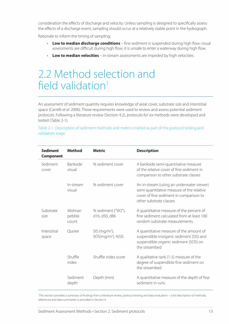
An assessment of sediment quantity requires knowledge of areal cover, substrate size and interstitial space (Cantilli et al. 2006). These requirements were used to review and assess potential sediment protocols. Following a literature review (Section 4.2), protocols for six methods were developed and tested (Table 2-1).
Table 2-1. Description of sediment methods and metrics trialled as part of the protocol testing and validation stage.
Sediment Component
Method Metric Description
Sediment cover
Bankside visual
% sediment cover A bankside semi-quantitative measure of the relative cover of fine sediment in comparison to other substrate classes
In-stream visual
% sediment cover An in-stream (using an underwater viewer) semi-quantitative measure of the relative cover of fine sediment in comparison to other substrate classes
Substrate size
Wolman pebble count
% sediment (“W2”), d16, d50, d86
A quantitative measure of the percent of fine sediment calculated from at least 100 random substrate measurements
Interstitial space
Quorer SIS (mg/m2), SOS(mg/m2), %SIS
A quantitative measure of the amount of suspendible inorganic sediment (SIS) and suspendible organic sediment (SOS) on the streambed
Shuffle index
Shuffle index score A qualitative rank (1-5) measure of the degree of suspendible fine sediment on the streambed
Sediment depth
Depth (mm) A quantitative measure of the depth of fine sediment in runs
consideration the effects of discharge and velocity. Unless sampling is designed to specifically assess the effects of a discharge event, sampling should occur at a relatively stable point in the hydrograph.
Rationale to inform the timing of sampling:
• Low to median discharge conditions – fine sediment is suspended during high flow; visual assessments are difficult during high flow; it is unsafe to enter a waterway during high flow.
• Low to median velocities – in-stream assessments are impeded by high velocities.
1This section provides a summary of findings from a literature review, protocol testing and data evaluation – a full description of methods, references and data summaries is provided in Section 4.

Sediment Assessment Methods • Section 2. Sediment protocols14
Protocol testing and validation involved a national-scale effort by 12 regional councils, Cawthron Institute (Cawthron), National Institute for Water and Atmospheric Research (NIWA), University of Canterbury and University of Otago over a period of six months and covering 264 river sites.
Results of the protocol testing and validation showed a high degree of consistency in the output provided by the different methods (Section 4.3.6). Sediment depth was the only metric not correlated with other measures of sediment. Results indicated that the bankside visual estimate of % sediment had the strongest and most consistent relationship with biological indicators of in-stream values (Section 4.3.8). The bankside visual estimate of % sediment was also strongly correlated with the more labour intensive in-stream visual estimate of % sediment (Section 4.3.6). The bankside method is likely to be a suitable measure for broad-scale state of the environment assessments. The bankside method provides a single numerical value, whereas the in-stream visual method includes multiple visual observations and therefore would be more suitable when a measure of error/variability is needed (Table 2-2).
Substrate size composition using a Wolman pebble count provides an assessment of % fine particles as well as other useful substrate composition data, for example, d50 (i.e., the median particle size) (Table 2-2). The Quorer method provides a quantitative measure of sediment in the surface and subsurface layers and as such could also be used to indicate the ‘embeddedness’ of particles and interstitial space. The Quorer method has several alternative measures that can be applied to assess suspendible sediment (i.e., SIS, SOS, suspendible benthic sediment volume (SBSV), Section 4.3.7). Whilst the Shuffle method was only weakly correlated with Quorer results, it does provide a rapid assessment of suspendible sediment in relation to amenity values (Section 4.3.6; see also Section 4.5.8).
Whilst the bankside visual estimate of % sediment was most consistently related to invertebrate metrics, all protocols trialled showed a significant correlation (p < 0.01) with the macroinvertebrate metrics of stream biotic health, the Macroinvertebrate Community Index (MCI) and/or the number of taxa belonging to the sensitive insect families Ephemeroptera, Plecoptera and Trichoptera (EPT) (Section 4.3.8).
Table 2-2. Recommended sediment protocols based on protocol testing and validation.
2.3 Recommended protocols
Type of assessment
Sediment component
Sediment cover Substrate composition
Interstitial space
State of the Environment
Bankside visual estimate
of % sediment
Wolman pebble count Quorer SIS
or Quorer SBSV
or Shuffle
Assessment of effects
In-stream visual
estimate of % sediment
Wolman pebble count Quorer SIS
Sediment depth (mm)
Sediment Assessment Methods • Section 2. Sediment protocols 15
Habitat Riffle Run Pool (Comments)
Habitat length (m)
% sediment
Ratio sand:finer(silt, clay, mud)
Photo (Yes/No)
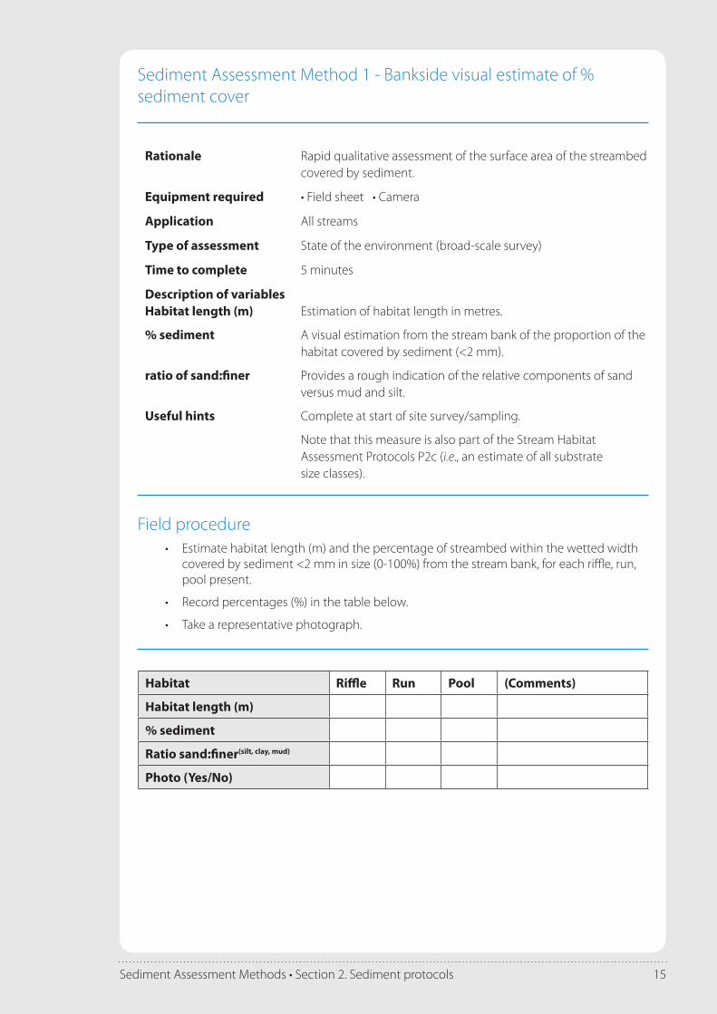
Rationale Rapid qualitative assessment of the surface area of the streambed covered by sediment.
Equipment required • Field sheet • Camera
Application All streams
Type of assessment State of the environment (broad-scale survey)
Time to complete 5 minutes
Description of variables Habitat length (m)
% sediment
ratio of sand:finer
Estimation of habitat length in metres.
A visual estimation from the stream bank of the proportion of the habitat covered by sediment (<2 mm).
Provides a rough indication of the relative components of sand versus mud and silt.
Useful hints Complete at start of site survey/sampling.
Note that this measure is also part of the Stream Habitat Assessment Protocols P2c (i.e., an estimate of all substrate size classes).
Sediment Assessment Method 1 - Bankside visual estimate of % sediment cover
Field procedure• Estimate habitat length (m) and the percentage of streambed within the wetted width
covered by sediment <2 mm in size (0-100%) from the stream bank, for each riffle, run, pool present.
• Record percentages (%) in the table below.
• Take a representative photograph.

Sediment Assessment Methods • Section 2. Sediment protocols16 Sediment Assessment Methods • Section 2. Sediment protocols16
Useful imagesRun, riffle and pool habitat locations (Image courtesy of Cathy Kilroy – from Biggs et al. 2002).
Notes:• The average value for each habitat present weighted by length is used to calculate %
sediment at the reach scale
• If all habitats are not present record % sediment for a run habitat only.
• The assessment of all substrate size classes can be obtained at the same time, but it is not necessary for the determination of % sediment cover. The table below can be used to assess all substrate size classes.
Habitat Riffle Run Pool (Comments)
Habitat length (m)
% mud/silt (<0.06 mm)
% sand (0.06-2 mm)
% fine gravel (2-16 mm)
% coarse gravel (16-64 mm)
% cobbles (64-256 mm)
% boulders (>256 mm)
% bedrock (layer of solid rock)

Sediment Assessment Methods • Section 2. Sediment protocols 17
Sediment Assessment Method 2 – In-stream visual estimate of % sediment cover
Rationale Semi-quantitative assessment of the surface area of the streambed covered by sediment. At least 20 readings are made within a single habitat
Equipment required • Underwater viewer - e.g., bathyscope (www.absolutemarine.co.nz) or bucket with a Perspex bottom marked with four quadrats • Field sheet
Application Hard-bottomed streams
Type of assessment Assessment of effects
Time to complete 30 minutes
Description of variables% sediment A visual estimate of the proportion of the habitat covered by
deposited sediment (<2 mm)
Useful hints Work upstream to avoid disturbing the streambed being assessed.Mark a four-square grid on the viewer to help with estimates – determine the nearest 5% cover for each quadrat.Calculate the average of all quadrats as a continuous variable following data entry.More than five transects may be necessary for narrow streams, to ensure 20 locations are sampled.
Field procedure• Locate five random transects along the run.
• View the streambed at four randomly determined locations across each transect, starting at the downstream transect.
• Estimate the fine sediment cover in each quadrat of the underwater viewer in increments (1, 5, 10, 15, 20 …100%).
• Record results in the table below.
• Repeat for four more transects so that 20 locations are sampled in total.
Note: Estimation of cover in each quadrat is important during training but may not be necessary for experienced viewers – instead one measurement per location could be recorded.
Sediment Assessment Methods • Section 2. Sediment protocols18 Sediment Assessment Methods • Section 2. Sediment protocols18
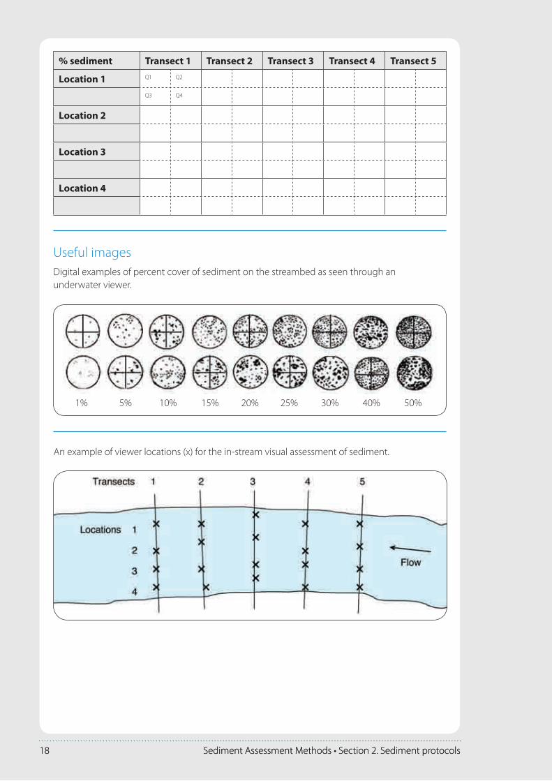
% sediment Transect 1 Transect 2 Transect 3 Transect 4 Transect 5
Location 1 Q1 Q2
Q3 Q4
Location 2
Location 3
Location 4
Useful imagesDigital examples of percent cover of sediment on the streambed as seen through an underwater viewer.
1% 5% 10% 15% 20% 25% 30% 40% 50%
An example of viewer locations (x) for the in-stream visual assessment of sediment.

Sediment Assessment Methods • Section 2. Sediment protocols 19
1% 1%
Real examples of percent cover of sediment on the streambed as seen through an underwater viewer.
5% 5%
10% 10%
15% 15%

Sediment Assessment Methods • Section 2. Sediment protocols20 Sediment Assessment Methods • Section 2. Sediment protocols20
25% 30%
40% 50%
90% 100%
20% 20%

Sediment Assessment Methods • Section 2. Sediment protocols 21
Sediment Assessment Method 3 – Wolman pebble count
Rationale Semi-quantitative assessment of the particle size distribution, including fine sediment, on the streambed. At least 100 particle measurements are made within a single habitat.
Equipment required • Gravelometer (www.envco.co.nz) or a ruler marked with a modified Wentworth scale (e.g., 2, 8, 16, 32, 64, 128, 256, >256 mm, bedrock) • Field sheet
Application Hard-bottomed streams
Type of assessment State of the environment (broad-scale survey)Assessment of effects
Time to complete 20 minutes
Description of variablesParticle size class The length of the particle B-axis in millimetres.
Useful hints Avoid bias in foot placement or in particle selection, i.e., be rigorous about selecting the particle in the middle of the front of the boot at regular paces across the stream.Assess any particles picked up – this should include silt/clay particles on top of larger particles.This measure is similar to that of the Stream Habitat Assessment Protocols P3c.
Field procedure• Sample beginning at the downstream end of a run and proceed across and upstream.
• Select particles at the front of your foot.
• Select at least 100 particles within the wetted width of a run.
• Use a gravelometer or a ruled rod, to measure the B-axis size class. The B-axis would prevent a particle from passing through a gravelometer/sieve.
• Record particle size classes (on a modified Wentworth scale) as tally marks in the table below. Note: Measurement of particle size is important during training but may not be necessary for experienced field staff – instead the descriptive table may be a useful guide.

Sediment Assessment Methods • Section 2. Sediment protocols22 Sediment Assessment Methods • Section 2. Sediment protocols22
Particle size class Count Description
Clay/silt(<0.06 mm)
Not gritty between fingers and hard to pick up but visible as particles
Sand (>0.06-2 mm)
Gritty between fingersSmaller than a match head
Small gravel (>2-8 mm)
Match head to little finger nail size
Small-Med Gravel(>8-16 mm)
Little finger nail to thumb nail size
Med-Large Gravel(>16-32 mm)
Thumb nail to golf ball size (or circle when thumb and index finger meet)
Large Gravel (>32-64 mm)
Golf ball to tennis ball size (or fist)
Small Cobble (>64-128 mm)
Tennis ball to softball size (or circle when thumb and index fingers of two hands meet)
Large Cobble(>128-256 mm)
Softball to basketball size
Boulders(>256 mm)
Basketball or greater
Bedrock Continuous layer of solid rock
Useful imagesB-axis of a pebble
“B” intermediate axis (mm)
“A” longest axis (mm)

Sediment Assessment Methods • Section 2. Sediment protocols 23
Sediment Assessment Method 4 – Resuspendible sediment (Quorer method)
Rationale Quantitative measure of total suspendible solids deposited on the streambed. Six samples are collected from a single habitat. Samples are processed in the laboratory for Total Inorganic/Organic Sediment by area (SIS and SOS, respectively) or Suspendible Benthic Solids by Volume (SBSV).
Equipment required • Cylindrical tube (e.g., 45 cm length of 35 cm diameter plumbing tube for gravel bed streams, or 60 cm length of 50 cm diameter metal tube for cobble bed streams) • 7 x >120 ml screw topped sample bottles • Stirrer • Ruler (e.g., broom handle marked with 1 cm graduations) • Field sheet
Application Hard-bottomed streams
Type of assessment State of the environment (broad-scale survey)Assessment of effects
Time to complete 30 minutes
Description of variablesSampleAverage water depth (m)Average stirred depth (m)
Sample numberThe average of five water depths inside the cylinder in metres.
The average of five water depths inside the cylinder in metres to the depth that the sediments were stirred. Measured after water sample collection.
Useful hints A split garden hose placed around the top of the tube aids with the insertion into coarse substrates. Welded handles at hand-height assist with use of large diameter corers used in cobble bed rivers.This method is not suitable for streambeds dominated by large boulders.Large cobbles can be removed from the corer prior to stirring.Do not over-fill sample bottles because they expand when frozen (samples should be frozen until analysis).
Field procedure• Collect a background water sample (i.e., control sample).
• Insert an open-ended cylinder into the streambed in a run and measure water depth at five random locations within the cylinder. Record average water depth. Stir the upper 5-10 cm of sediment for 15 seconds.
• Collect a sample of slurry (dirty water) and label.
• Estimate average stirred depth (sediment + water).
• Repeat Quorer method at five more locations.
• Freeze the six slurry samples and one background sample per site until laboratory analysis.

Sediment Assessment Methods • Section 2. Sediment protocols24 Sediment Assessment Methods • Section 2. Sediment protocols24
Sample Average water depth (m) Average stirred depth (m)
Control na na
1
2
3
4
5
6
Notes• Suspendible inorganic sediment (SIS) and suspendible organic sediment (SOS) are
determined using the standard protocol for Total Suspended Solids (TSS method 2540D in APHA 1998) and Volatile Suspended Solids (VSS method 2540E in APHA 1998).
o SIS (g/m2) = (TSS(sample – control) – VSS(sample – control)) x average depth (m) in cylinder
o SOS (g/m2) = VSS(sample – control) x average depth (m) in cylinder
• Stirred depth (m) is used to calculate SIS or SOS in g/m3.
• Suspendible benthic sediment volume (SBSV) is determined using a settling assay (See Appendix 6.4 for details).
• The average value is calculated for each site.

Sediment Assessment Methods • Section 2. Sediment protocols 25
Sediment Assessment Method 5 - Resuspendible sediment (Shuffle index)
Field procedure• Place a white tile on the streambed in a run, and measure/estimate water depth and
velocity at this point.
• Stand 3 m upstream of the tile and disturb the streambed by moving feet vigorously for five seconds.
• Allocate a score from 1-5 depending on the visibility and duration of the resulting plume in relation to the white tile downstream.
• Take a photo record of the plume where possible.
• Repeat this process twice upstream.
Rationale Rapid qualitative assessment of the amount of total suspendible solids deposited on the streambed. A score from 1-5 is assigned, where 1 = little/no sediment and 5 = excessive sediment.
Equipment required • Camera • 10 cm x 10 cm white tile • Field sheet
Application All streams
Type of assessment State of the environment (broad-scale survey)Assessment of effects (as support variable)
Time to complete 5 minutes
Description of variablesWater depth (m)Water velocity (fast/medium/slow)ScorePhoto
Depth of water in metres at tile locationWater velocity at tile location
A value of 1-5Indication of whether a photo record was obtained (preferably ‘Yes’)
Useful hints This method is best applied in an area where flow is between 0.2 0.6 m/sec and depth is between 20 and 50 cm.Depth and velocity may be estimated and are mainly recorded to ensure the method was applied in appropriate and comparable conditions. Photos could be taken by a second team member on the stream bank. Best completed at the end of sampling.The average score is calculated for each site.
Sample Water Depth (m)
Water velocity (fast/medium/slow)
Score Photo (yes/no)
1
2
3

Sediment Assessment Methods • Section 2. Sediment protocols26 Sediment Assessment Methods • Section 2. Sediment protocols26
Useful imagesResuspendible sediment index examples.
Score 1: No or small plume
Score 2: Plume briefly reduces visibility at tile
Score 3: Plume partially obscures tile but quickly clears
Score 4: Plume partially to fully obscures tile but slowly clears
Score 5: Plume fully obscures tile and persists even after shuffling ceases

Sediment Assessment Methods • Section 2. Sediment protocols 27
Sediment Assessment Method 6 –Sediment depth
Rationale Quantitative assessment of the depth of sediment in a run habitat. At least 20 readings are made within a single habitat
Equipment required • Ruler or ruled rod • Field sheet
Application Hard-bottomed streams
Type of assessment Assessment of effects
Time to complete 30 minutes
Description of variablesSediment depth (mm) A measure of the depth of sediment (mm).
Useful hints Determine the sampling grid first to ensure an even cover of edge and midstream locations.Move upstream to avoid disturbing the streambed being assessed.Calculate the average depth for each site.This method is usually only suitable when fine sediment is visible from the stream bank.
Field procedure• Start downstream and randomly locate five transects along the run.
• Measure the sediment depth (mm) at four randomly determined locations across each transect and record depth in the table below.
Depth (mm) Transect 1 Transect 2 Transect 3 Transect 4 Transect 5
Section 1
Section 2
Section 3
Section 4

Sediment Assessment Methods • Section 2. Sediment protocols28

Section 3Sediment guidelines

30 Sediment Assessment Methods • Section 3. Sediment guidelines
3 Sediment Guidelines
This section outlines the guiding principles to applying sediment guidelines, such as their foundation on values based assessments and their application in hard-bottomed streams during low flow.
Numerical guideline values are recommended for the protection of biodiversity, fish spawning habitat and in-stream amenity values.
A summary of findings from a literature review, a survey and data analysis to inform guideline development is provided. Reference to scientific literature has been omitted for ease of reading – for more detail readers are referred to Sections 4.1, 4.4 and 4.5.
3.1 Guiding principles
3.1.1 Values-based assessmentThere is a common acceptance that excessive fine sediment deposited on stream and river beds can adversely affect a number of environmental and community values, including, but not restricted to, ecosystem health, amenity and recreational values. However, there is currently little guidance about what constitutes acceptable and unacceptable levels of sediment in relation to the different in-stream values.
The key question driving the development of these guidelines is:
What level of sedimentation corresponds to a significant adverse effect on the different in-stream values?
The aim of these guidelines is to use the best current scientific information and knowledge available nationally and internationally to answer this question in relation to three key in-stream values identified by the regional councils (Section 1.4; see also Appendix 6.1):
• macroinvertebrate communities health, as an indicator of overall aquatic ecosystem health
• trout spawning
• aesthetic, amenity and contact recreation values.
These guidelines are formulated as numerical thresholds, representing levels of in-stream sedimentation beyond which specific in-stream values become impaired.
Rationale informing guideline development:
• Guidelines relate to values – proposed guidelines provide a level of protection of the identified primary in-stream values (invertebrates, fish, and aesthetics).
3.1.2 Hard- versus soft-bottomed streamsWhether a stream is naturally dominated by fine sediment is dependent on a number of factors including stream size, slope, rainfall, catchment vegetation and geology. Streams naturally dominated by sediment are usually very small streams with low slopes and low rainfall on sandy soils. Such ‘soft-bottomed’ streams currently account for approximately 20% of the length of rivers in New Zealand, according to Freshwater Ecosystems of New Zealand (FENZ) classification (Leathwick et al. 2011). Whereas, predictions from GIS models suggest less than 2% of all NZ streams would have greater than 50% fine sediment cover in the absence of human land-use activities (Section 4.5.4). Together these analyses indicate that the majority of streams in New Zealand are, or should be ‘hard-bottomed’,

31Sediment Assessment Methods • Section 3. Sediment guidelines
dominated by relatively coarse (gravel or larger) substrate.
During the protocol development stage sediment depth was trialled as a potential metric to assess naturally soft-bottomed streams. However, sediment depth was poorly related to invertebrate biotic metrics, possibly because many of the indicators used to assess stream condition in New Zealand are developed primarily for application in hard-bottomed streams, for example %EPT. Sediment depth data was also not as abundant as other protocol data.
Thus these guidelines focus on hard-bottomed streams and assume that an increase in sediment is detrimental to fauna and flora naturally occurring in hard-bottomed streams. However, some protocols reviewed in Section 4.2 may be applicable for assessing sediment accumulation in soft-bottom streams (e.g., volume of sediment in pools). Guideline values are not provided for these untested methods.
Rationale informing guideline development:
• Hard-bottomed streams – majority of waterways in New Zealand are or should be dominated by coarse substrate.
3.1.3 Accounting for temporal and spatial variabilityNew Zealand is a geologically young and tectonically active country subject to strong erosive elements (wind, rain) and land forming processes (tectonic uplift, volcanism and earthquakes). New Zealand streams can be subject to high sediment loads on a continual or episodic nature and some river systems have among the highest sediment bed loads recorded globally (Hicks et al. 2000). Furthermore, human land-use activities can accelerate in-stream sediment delivery and alter downstream transportation. For example, a storm event can lead to land slumping that delivers sediment to a stream; the degree of slumping can be amplified due to vegetation clearance for agriculture, while water abstraction can reduce the power of a stream to redistribute sediment.
The above example illustrates the need to consider temporal and spatial variability in sediment distribution and accumulation when applying sediment guidelines. Therefore, it is important to determine ‘excess’ sediment in relation to what would occur naturally, i.e., in respect to a reference condition. It is also important to be wary of undertaking sediment assessments at times of active sediment movement, for example, immediately after periods of high flow.
Rationale informing guideline development:
• Comparison to reference – New Zealand streams vary a lot over space and time. While an upper limit may be applicable to protect certain values in all waterways, the degree of departure from a reference state will provide a more sensitive assessment of sediment impact.
3.2 Determining sediment guideline values2
An evidence-based approach was used to develop guidelines for sediment quantity, based on reported relationships and available data. This is sometimes referred to as ‘weight-of-evidence’ or ‘consensus-based’ approach and is widely used to define guideline values and inform decision-making processes in regards to sediment quality (e.g., MacDonald et al. 2000; Burton et al. 2002).
The methods used to determine sediment guidelines included:
2This section provides a summary of findings from a literature review, survey and data analysis to inform guideline development. Reference to scientific literature has been omitted for ease of reading. For more detail readers should refer to sections 4.4 and 4.5.

32 Sediment Assessment Methods • Section 3. Sediment guidelines
• a review of existing guidelines (Section 4.4)
• a review of quantitative relationships between sediment and in-stream values (Sections 4.1 and 4.5.7)
• correlative analyses among sediment metrics (Section 4.5.2)
• linear regression analyses among sediment metrics and biotic variables (Section 4.3.8)
• data mining to inform reference state (Section 4.5.5)
• boosted regression tree model to inform reference state (Section 4.5.4)
• survey of amenity values (Section 4.5.6).
A review of existing sediment guidelines for waterways identified a wide range in sediment criteria and standards because of a wide range in definitions of deposited fine sediment (i.e., anywhere from <0.85 mm to <6.4 mm in size) and methods used to measure sediment (e.g., Wolman pebble counts, embeddedness). Also, sediment guidelines have been developed to protect a range of values. Generally, sediment guidelines include an absolute upper limit and a target deviation from reference. In North America, upper limits range from less than 3% to less than 30% sediment with less than 5% to less than 27% recommended deviation from reference.
Environment Canterbury Regional Council is the only New Zealand authority to currently include sediment guidelines in regional planning, recommending between 10% and 40% absolute sediment cover, depending on the management purposes defined in each water quality management unit .
A review of quantitative relationships between sediment and in-stream values in New Zealand showed that sediment directly affects invertebrate community composition, EPT taxa richness and abundance, specific taxa density and invertebrate drift. Anywhere between 10% and 10-fold increases in sediment resulted in noticeable invertebrate responses, with changes amplified over time. Few quantitative relationships have been observed between native fish and deposited sediment. International literature suggests ideal sport fish habitat (i.e., salmonids) has less than 10% sediment, but greater than 20% sediment will result in fish egg mortality.
Correlative analyses among sediment metrics showed that all visual estimates of sediment cover were strongly correlated, i.e., in-stream visual, and bankside visual at a reach or run scale. This suggests that guidelines developed for sediment cover can be assessed using any visual assessment method. Quorer metrics were related to visual estimates of sediment cover at a run scale, but not at a reach scale. All other sediment metrics were related to each other except % sediment calculated from Wolman pebble counts and sediment depth. Results demonstrated the interdependence of sediment components, i.e., cover, substrate size and suspendible sediment.
Linear regression analyses among sediment metrics and biotic variables showed few predictive relationships and a wide range in biotic values at low values of sediment. A linear relationship between bankside visual % sediment and MCI suggested a negative value of sediment at 120 MCI (i.e., MCI value indicative of good health). A negative linear relationship between bankside visual % sediment and %EPT richness suggested a value of 7% sediment at 50% EPT (i.e., EPT value potentially indicative of good health). A negative linear relationship between SIS (log-transformed) and MCI suggested a value of 22 g/m2 at 120 MCI. A negative linear relationship between sediment depth (log-transformed) and the total number of invertebrate taxa and EPT richness was also observed.
Data mining to inform reference state involved viewing the distribution of sediment data to determine the 75th percentile for sites with greater than 80% native vegetation in their catchments, and the 75th percentile for sites with greater than 120 MCI and greater than 50% EPT. These approaches resulted in a similar value for each of the sediment metrics (Table 3-1).

33Sediment Assessment Methods • Section 3. Sediment guidelines
Table 3-1. Sediment reference values derived from two approaches to examine the distribution of sediment data collated to develop sediment guidelines.
Summary of 75th percentile values>80% native vegetation >120 MCI >50% EPT
% sediment (bankside visual reach scale) 15 20 20
% sediment (bankside visual run scale) 20 20 20
% sediment (in-stream visual) 17 13 17
% sediment (Wolman pebble count) 17 8 20
SIS (g/m2) 405 429 953
SOS (g/m2) 28 43 69
%SIS 91 94 94
Shuffle index score 2 2 3
Sediment depth (mm) 9 4 63
SIS = Suspendible inorganic sediment, SOS – suspendible organic sediment, %SIS = percentage of suspendible sediment that is inorganic
A boosted regression tree model to inform reference state was used to make national predictions of sediment cover in the absence of land-use impacts. Percent sediment data from the New Zealand Freshwater Fish Database (NZFFD) was used along with land-use and environmental descriptors for each stream reach from FENZ. The model predicted a current national average of 29% sediment cover, but when the influence of land-use was factored out, the model predicted a national average of only 8% sediment cover. A range in predicted ‘reference’ sediment conditions was evident for different stream types as classified by FENZ 20-level stream types, for example, 29.4% sediment for Group B (i.e., small warm coastal streams) down to 2.4% sediment for Group S (i.e., cold steep mountainous streams).
Finally, a survey of amenity values was conducted to inform the level of sediment acceptable for swimming and recreation. Results suggested that amenity value changes from acceptable to unacceptable between 12% and 27.5% sediment cover and swimming value decreases from acceptable to unacceptable between a Shuffle index score of 2 and a Shuffle index score of 3.
Information from all of the above approaches was used to inform recommended guidelines. For biodiversity values, weight was given to the results of data mining to inform absolute limits because the results of the regression analyses were weak. The national sediment model provides guidance for assessing deviation from predicted reference. For salmonid values, weight was given to relationships reported in the literature. For amenity values, weight was given to results of the user survey.
3.3 Recommended GuidelinesThe following are recommended guidelines for assessing the effects of deposited fine sediment on the in-stream values of hard-bottomed streams.

34 Sediment Assessment Methods • Section 3. Sediment guidelines
Sediment measure
Sediment value
Core method Supporting data
Application
Sediment cover
(%)
< 20% OR within
10% cover of
reference
Bankside visual
estimate
Photo State of the
environment
reporting
< 20% OR within
10% cover of
reference
In-stream visual
estimate
Photo Assessment of
effects
Substrate size
(%)
< 20% OR within
10% cover of
reference
Wolman pebble
count
State of the
environment
reporting OR
Assessment of
effects
Suspendible
sediment
< 450 g/m2 Quorer (SIS) State of the
environment
reporting OR
Assessment of
effects
In-stream value = Biodiversity*
[* includes native fish on the assumption that benthic invertebrates are their primary food source]
In-stream value = Salmonid spawning habitat
Sediment measure
Sediment value
Core method Supporting data
Application
Sediment cover
(%)
< 20% OR within
10% cover of
reference
Bankside visual
estimate
Photo State of the
environment
reporting
< 20% OR within
10% cover of
reference
In-stream visual
estimate
Photo Assessment of
effects
Substrate size
(%)
< 20% Wolman pebble
count
State of the
environment
reporting OR
Assessment of
effects

35Sediment Assessment Methods • Section 3. Sediment guidelines
In-stream value = Amenity
Sediment measure
Sediment value
Core method Supporting data
Application
Sediment cover
(%)
< 25% Bankside visual
estimate
Photo State of the
environment
reporting
< 25% In-stream visual
estimate
Photo Assessment of
effects
Suspendible
sediment
< 3 Shuffle index Photo State of the
environment
reporting
The following guidelines are recommended; that sediment should not exceed either:
1) 20% cover or 450 g/m2 (SIS) to protect stream biodiversity and fish (native and trout) habitat.
2) 25% cover or Shuffle index score of 3 to protect stream amenity.
We recommend that these numerical guidelines provide upper limits on the amount of fine sediment that will affect in-stream values, i.e., any amount of sediment greater than 20% cover will detrimentally affect biodiversity and fish habitat. Note that there are likely to be lower limits at which in-stream value levels will be negatively affected by sediment. The available data makes it difficult to locate those limits, so for this reason it is recommended that a comparison of sediment values with a reference condition is applied.

36 Sediment Assessment Methods • Section 3. Sediment guidelines

Section 4Supporting
Information

38 Sediment Assessment Methods • Section 4. Supporting information
4 Supporting Information
This section contains detailed information used to support the development of protocols and guidelines to assess the effects of sediment on in-stream values.
Included are literature reviews on sediment effects on biota and sediment assessment methods, and a review of existing sediment guidelines.
Comprehensive details on protocol testing and validation, guideline development including the prediction of reference values, and other useful things we learnt along the way are also included.
4.1 Review of sediment effects on biota and in-stream values
4.1.1 Benthic invertebratesThe most commonly inferred causal pathway for invertebrate response to sediment is a change in habitat. By definition, benthic invertebrates live on or in the streambed and hence any change to this habitat will directly affect the invertebrate community. However, there is a wide range of responses of benthic invertebrates to increased sediment including changes in invertebrate feeding and growth, behaviour, community composition, diversity and abundance (Ryan 1991; Waters 1995; Wood & Armitage 1997; Crowe & Hay 2004).
Invertebrate feeding can be directly affected by clogging of feeding apparatus (i.e., impeded filter-feeding) and by loss of suitable habitat for attachment or feeding (Ryan 1991). Indirect effects on invertebrate feeding may also occur, via changes in food source and nutritional content as well as the adherence of toxicants to sediment (Ryder 1989; Collier 2002).
Sediment deposition can alter invertebrate behaviour. Interstitial spaces between substrata are used by invertebrates to avoid predators and the scouring effects of high flow (Sedell et al. 1990). Increased sediment deposition can lead to the short-term increase in invertebrate drift (Larsen & Omerod 2009; Molinos & Donohue 2009), and in the long term, invertebrate recolonisation through upstream movement may also be disrupted by large-scale fine sediment accumulation (Luedtke & Brusven 1976).
Ultimately the clogging of both surface and subsurface habitats by sediment leads to changes in invertebrate density and community composition (Waters 1995; Matthaei et al. 2006). As the level of sediment increases, taxa that favour stony habitat such as EPT taxa (Ephemeroptera, Plecoptera and Trichoptera) are replaced by burrowing taxa such as chironomids and worms (Wood & Armitage 1997; Rabeni et al. 2005; Townsend et al. 2008).
In New Zealand, there is more information available on the quantitative relationships between sediment and benthic invertebrates than for other in-stream values (Table 4-1).

39Sediment Assessment Methods • Section 4. Supporting information
Table 4-1 Quantitative relationships that have been documented between proportions of sediment and invertebrate populations in New Zealand (adapted from Crowe & Hay 2004).
Taxon / Community descriptor
Experimental method
Sediment size
Quantitative relationship established
Source
Deleatidium Introduced
substrates
in relatively
‘sediment-free’
stream
0.5-2 mm 12-17% increase
in interstitial fine
sediments resulted
in a 27-55% decrease
in abundance
Ryder (1989)
Deleatidium,
hydrobiosid
caddisflies
Sediment
additions into
stream section
0.125-1 mm Abundances
decreased as
amount of fine
sediment increased
Ryder (1989)
Elmidae,
Oligochaeta,
Potamopyrgus
antipodarum
Sediment
additions into
stream section
0.125-1 mm No significant
change in
abundance
Ryder (1989)
Trichoptera,
Chironomidae
Introduced
substrates
in relatively
‘sediment-free’
stream
0.5-2 mm Generally more
common on
substrates without
interstitial fine
sediments
Ryder (1989)
Pycnocentrodes,
Austrosimulium, P.
antipodarum
Introduced
substrates
in relatively
‘sediment-free’
stream
0.5-2 mm Abundance
not affected by
increased interstitial
fine sediments
Ryder (1989)
Elmidae Introduced
substrates
in relatively
‘sediment-free’
stream
0.5-2 mm Abundance
increased as amount
of interstitial fine
sediments increased
Ryder (1989)
Total invertebrate
abundance
Introduced
substrates
in relatively
‘sediment-free’
stream
0.5-2 mm 12-17% increase
in interstitial fine
sediments resulted
in a 16-40% decrease
in abundance
Ryder (1989)

40 Sediment Assessment Methods • Section 4. Supporting information
Taxon / Community descriptor
Experimental method
Sediment size
Quantitative relationship established
Source
Total invertebrate
density, biomass,
taxa richness
Survey of 88 NZ
rivers
Silt <0.063
mm, sand
0.063-2
mm.
Decreased
invertebrate
density, biomass
and taxa richness
in rivers with high
proportions of
silt and sand in
surface sediments,
c.f. communities
in rivers with
coarser substrate
compositions
Quinn & Hickey (1990)
Total invertebrate
abundance, taxa
richness
Sediment
additions into
stream sections
<4 mm Following 21
days exposure,
total invertebrate
abundance and
taxa richness
had decreased
significantly (c.f.
controls). Mean
total number
of individuals
decreased by 40-
55%, and mean taxa
richness decreased
by 15-30%
Dunning (1998)
Helicopsyche,
Zephlebia
Sediment
additions into
stream sections
<4 mm Following 21
days exposure,
abundance of
Zephlebia and
Helicopsyche
had decreased
significantly (c.f.
controls)
Dunning (1998)

41Sediment Assessment Methods • Section 4. Supporting information
Taxon / Community descriptor
Experimental method
Sediment size
Quantitative relationship established
Source
Diptera Sediment
additions into
stream sections
<4 mm Following 21
days exposure,
abundances had
increased (c.f.
controls), but
not statistically
significant
Dunning (1998)
Potamopyrgus
antipodarum,
Elmidae
Sediment
additions into
stream sections
<4 mm Following 21
days exposure,
abundances had
not changed
significantly (c.f.
controls) for either
Dunning (1998)
% EPT taxa, QMCI,
MCI
Sediment
additions into
stream sections
<4 mm Following 21 days
exposure, %EPT
taxa and QMCI
had decreased
significantly (c.f.
controls), whereas
MCI showed no
significant change
Dunning (1998)
Deleatidium drift Sediment
additions to
artificial channels
containing
cobble substrate
and established
algae and
invertebrate
communities.
Deleatidium
added to
channels after
sediment
additions.
<2 mm 16% increase in
interstitial fine
sediment resulted in
a 80% mean increase
in numbers of
drifting Deleatidium
Suren & Jowett (2001)

42 Sediment Assessment Methods • Section 4. Supporting information
Taxon / Community descriptor
Experimental method
Sediment size
Quantitative relationship established
Source
Paracalliope
fluviatilis, Oxyethira
albiceps, Hydrobiosis
sp. and chironomid
larvae drift
Sediment
additions to
artificial channels
containing
cobble substrate
and established
algae and
invertebrate
communities
<2 mm 16% increase in
interstitial fine
sediment resulted in
a doubling of drift
rates
After 3 days,
abundances
of chironomid,
Oxyethira and
Hydrobiosis larvae
were significantly
lower in sedimented
channels
Suren & Jowett (2001)
Chironomid
emergence, diurnal
drift patterns
Sediment
additions to
artificial channels
containing
cobble substrate
and established
algae and
invertebrate
communities
<2 mm 16% increase in
interstitial fine
sediment had no
significant effect
on chironomid
emergence or
diurnal drift patterns
Suren & Jowett (2001)
Ephemeroptera,
Trichoptera
Longitudinal
and temporal
sampling of
anthropogenic
point-source
inputs of fine
sediment to a
river
‘Sand’ A c. 10-fold increase
in percentage cover
by sand (c. 5%
cover at upstream
control vs. 50-54%
at downstream
sites), resulted in a
30-75% reduction in
Ephemeroptera and
a 70-80% reduction
in Trichoptera
Cottam & James (2003)

43Sediment Assessment Methods • Section 4. Supporting information
Taxon / Community descriptor
Experimental method
Sediment size
Quantitative relationship established
Source
Diptera, Oligochaeta Longitudinal
and temporal
sampling of
anthropogenic
point-source
inputs of fine
sediment to a
river
‘Sand’ A c. 10-fold increase
in percentage cover
by sand resulted
in a 0.5 to 2.4-fold
increase in Diptera
and a 1 to 8-fold
increase Oligochaeta
Cottam & James (2003)
Taxa richness, EPT
richness
Longitudinal
and temporal
sampling of
anthropogenic
point-source
inputs of fine
sediment to a
river
‘Sand’ A c. 10-fold increase
in percentage cover
by sand resulted in
a 40-50% reduction
in median taxa
richness, and a 25-
50% reduction in
median EPT richness
Cottam & James (2003)
Potamopyrgus
antipodarum &
Deleatidium
Laboratory
preference
trials using
cobbles subject
to differing
sediment and
algae treatments
<0.5 mm Both species
preferred a sediment
contaminated
version of their
respective food
source over
alternative alga
Suren (2005)
Invertebrate density,
taxa richness, EPT
richness, specific
taxa density
Sediment
addition to
natural stream
channels
<2 mm Decrease in taxa
richness, EPT
richness and specific
taxa density. Effects
most significant
in pasture streams
where pre-
treatment richness
and diversity were
highest.
10/20 taxa
unaffected
Matthaei
et al. (2006)

44 Sediment Assessment Methods • Section 4. Supporting information
Taxon / Community descriptor
Experimental method
Sediment size
Quantitative relationship established
Source
Taxa richness, EPT
richness
Sediment
addition to
natural stream
channels
<2 mm
(mean = 0.2
mm)
Increase from 35%
to 83% fine cover
correlated with
increased taxa and
EPT richness
Townsend
et al. (2008)
Invertebrate density,
EPT richness
Spatial survey of
32 streams
<1 mm With an increase
in fine sediment
cover there was
an increase in
invertebrate density,
and a decrease in
EPT taxa richness
Townsend
et al. (2008)
4.1.2 FishSediment influences fish directly through physical effects and indirectly through impacts on habitat and food supply. Most physical effects are attributed to the gill damaging properties of suspended sediment, which can limit fish growth and make fish susceptible to disease (Waters 1995). Suspended sediment can also reduce the visual foraging efficiency of fish including the avoidance of highly turbid rivers by migratory species (Boubée et al. 1997; Rowe & Dean 1998). In comparison, deposited sediment limits the amount of habitat available for spawning and can reduce the viability of egg survival (Wood & Armitage 1997; Harvey et al. 2009). Salmonids are particularly susceptible to excess sediments that suffocate eggs in redds (Hay 2005).
Deposited fine sediment also reduces the amount of habitat and cover available to juvenile and adult fish. Native fish species favour habitats with large interstices (e.g., gaps between cobbles) which are important for refuge (Jowett & Boustead 2001; McEwan 2009). In terms of food availability, sediment can alter the macroinvertebrate community in favour of less preferred food items for some fish species, i.e., a reduction in drifting species. As such, sediment can affect the small-scale distribution of fishes and hence fish density and richness.
Information on the effects of deposited sediment on native New Zealand fish is limited to studies of habitat and food preferences. For many species information is anecdotal at best. Few quantitative relationships have been reported, although there are some established relationships between suspended sediment and fish populations (Table 4-2).

45Sediment Assessment Methods • Section 4. Supporting information
Table 4-2. Quantitative and observational relationships that have been documented between proportions of deposited sediment, suspended sediment and fish populations in New Zealand.
Taxon / Community descriptor
Experimental method
Fine sediment metric
Relationship established
Source
Upland bullies
(adult)
Sediment
addition (12.4 kg/
m2) in artificial
stream
96% <2
mm and
4% >2 mm
50% decline in
numbers after six
days
Jowett & Boustead (2001)
Redfin bully,
Shortjaw kokopu
Survey of a
natural stream
0.5 mm
as part of
substrate
index
Presence
associated with
gravel and larger
substrates in day
and gravel and
smaller substrates
at night
McEwan (2009)
Koaro Survey of a
natural stream
0.5 mm
as part of
substrate
index
Presence
associated with
larger substrates
day and night
McEwan (2009)
Banded kokopu Spotlight survey
of a natural
stream
2 mm and
as part of
a substrate
index
Size-based
microhabitat
selection observed
with smaller fish
associated with
smaller substrate
sizes
Akbaripasand et al. (2011)
Banded kokopu Laboratory
preference trials
17 NTU
25 NTU
50% avoidance
response
Boubée et al. (1997)
Redfin bully Laboratory
preference trials
1110 NTU No avoidance
behaviour
Boubée et al. (1997)
Koaro Laboratory
preference trials
70 NTU 50% avoidance
response
Boubée et al. (1997)
Inanga Laboratory
preference trials
420 NTU 50% avoidance
response
Boubée et al. (1997)
Large eels Laboratory
preference trials
1110 NTU No avoidance
behaviour
Boubée et al. (1997)

46 Sediment Assessment Methods • Section 4. Supporting information
Taxon / Community descriptor
Experimental method
Fine sediment metric
Relationship established
Source
Smelt Laboratory tank
experiment
640 NTU 59% reduction in
feeding rate
Rowe & Dean (1998)
Banded kokopu Laboratory tank
experiment
20 NTU 45% reduction in
feeding rate
Rowe & Dean (1998)
Redfin Bully Laboratory tank
experiment
Between
40 and 640
NTU
50% reduction in
feeding rate
Rowe & Dean (1998)
Banded kokopu Laboratory tank
experiment
120 mg/l
suspended
solids
60% avoidance
response
Rowe et al. (2000)
Banded kokopu Suspended
sediment
addition to
natural stream
channel
25 NTU 40% moved
upstream when
NTU was below 25
NTU, after which
there was 0%
movement
Richardson et al. (2001)
Longfin eel, shortfin
eel, Common bully,
Redfin bully, Bluegill
bully, Torrentfish,
Inanga, Smelt, Koaro
Survey of natural
stream channel
Clarity Range in clarity
values explained
40% variation in
species richness
Richardson & Jowett (2002)
Smelt Laboratory tank
experiment
1700 to
3000 NTU
50% mortality after
24 hours
Rowe et al. (2004)
Inanga Laboratory tank
experiment
1750 to
2100 NTU
50% mortality after
24 hours
Rowe et al. (2004)
Banded kokopu Laboratory tank
experiment
43000 NTU 10% mortality after
24 hours
Rowe et al. (2009)
Redfin Bully Laboratory tank
experiment
43000 NTU 15% mortality after
24 hours
Rowe et al. (2009)
4.1.3 Recreational and aesthetic valuesExcess fine sediment can detrimentally affect the amenity value of rivers and streams including recreational use for swimming and other water sports, fishing and general aesthetics. Poor water clarity associated with suspended sediments, or bed sediments that are suspended on contact, usually results in a negative experience for swimmers, as does the ‘feel’ of fine sediment under the toes.

47Sediment Assessment Methods • Section 4. Supporting information
Aesthetic value can be a very personal experience and difficult to measure. However, studies have demonstrated how people prefer streams with good visual clarity for bathing (Smith et al. 1995) and low turbidity for aesthetic value (Pflüger et al. 2010). This is reflected in surface water quality guidelines that set minimum clarity levels for recreational water use (e.g., >1.6 m black disc visibility, MfE 1994). However, currently there are no quantitative relationships between deposited fine sediment and recreational value.
4.2 Review of sediment assessment methodsA wide range of methods have been applied in New Zealand and elsewhere to quantify sediment in rivers and streams (Bunte & Abt 2001; Meredith et al. 2003; Sutherland et al. 2008). Although it is recognized that there is not necessarily one universal method to assess fine sediment in streams, some standardisation appeared necessary and was a key reason for initiating this project. Different properties of sediment may relate more informatively to some in-stream values compared to others. A conceptual model of the proximate stressors and causal pathways that lead to a response in benthic biota due to increased deposited sediments can help identify the required focus of sediment metrics (Figure 4-1). This conceptual model suggests that at minimum sediment metrics should assess substrate size, interstitial space and the coverage of fine sediment if all components of the issue are being evaluated. However, the model does not take into account the interdependence of these components.
Figure 4-1. Conceptual model depicting the relationship between increased deposited sediment and the effects on in-stream biota (adapted from Cantilli et al. 2006).
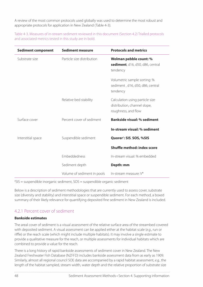
48 Sediment Assessment Methods • Section 4. Supporting information
A review of the most common protocols used globally was used to determine the most robust and appropriate protocols for application in New Zealand (Table 4-3).
Table 4-3. Measures of in-stream sediment reviewed in this document (Section 4.2) Trialled protocols and associated metrics tested in this study are in bold.
Sediment component Sediment measure Protocols and metrics
Substrate size Particle size distribution Wolman pebble count: % sediment, d16, d50, d86, central
tendency
Volumetric sample sorting: %
sediment , d16, d50, d86, central
tendency
Relative bed stability Calculation using particle size
distribution, channel slope,
roughness, and flow
Surface cover Percent cover of sediment Bankside visual: % sediment
In-stream visual: % sediment
Interstitial space Suspendible sediment Quorer#: SIS, SOS, %SIS
Shuffle method: index score
Embeddedness In-stream visual: % embedded
Sediment depth Depth: mm
Volume of sediment in pools In-stream measure: V*
#SIS = suspendible inorganic sediment, SOS = suspendible organic sediment
Below is a description of sediment methodologies that are currently used to assess cover, substrate size (diversity and stability) and interstitial space or suspendible sediment. For each method, a boxed summary of their likely relevance for quantifying deposited fine sediment in New Zealand is included.
4.2.1 Percent cover of sedimentBankside estimates
The areal cover of sediment is a visual assessment of the relative surface area of the streambed covered with deposited sediment. A visual assessment can be applied either at the habitat scale (e.g., run or riffle) or the reach scale (which might include multiple habitats). It may involve a single estimate to provide a qualitative measure for the reach, or multiple assessments for individual habitats which are combined to provide a value for the reach.
There is a long history of rapid bankside assessments of sediment cover in New Zealand. The New Zealand Freshwater Fish Database (NZFFD) includes bankside assessment data from as early as 1909. Similarly, almost all regional council SOE data are accompanied by a rapid habitat assessment, e.g., the length of the habitat sampled, stream width, water depth and the relative proportion of substrate size

49Sediment Assessment Methods • Section 4. Supporting information
cover are all metrics readily recorded. Since the development of Stream Habitat Assessment Protocols (Harding et al. 2009) a number of councils are routinely recording this information. Bankside visual assessments result in a single measure for a habitat or reach.
Metric Percent cover of fines
Method Bankside visual assessment
Nature of data Semi-quantitative
Recommended measure SOE monitoring
In-stream estimates
An underwater viewer is used to systematically sample multiple patches of the streambed in an in-stream visual assessment (Figure 4-2). Multiple estimates of fine sediment cover are averaged to provide a measure for a given habitat or reach. Protocols for this technique have been developed independently in New Zealand; in the Motueka River (Phillips & Basher 2005) and in Otago (Matthaei et al. 2006). Matthaei et al. (2006) detected a significant biological response to sedimentation assessed using this technique. Best results would seem to be obtained when the resolution of measurements is small enough to detect changes but large enough to minimise user bias (i.e., choosing measurements which are multiples of 5%). As with other patch-scale assessments, replication needs to be sufficient to incorporate substrate variability (i.e., more samples are required in heterogeneous substrates). These visual classification techniques generally require a high level of training to minimise user error (Latulippe et al. 2001). Dividing the viewer into smaller fields (Figure 4-2) helps to decrease user bias and are useful during user training, but do not necessarily improve the accuracy of visual assessment (Buffington & Montgomery 1999a).
Figure 4-2. Photos of an underwater viewer used to assess fine sediment cover.
Metric Percent cover of fines
Method In-stream visual assessment with an underwater viewer
Nature of data Semi-quantitative
Recommended measure SOE monitoring
Effects-based assessments
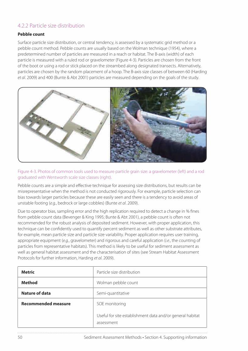
50 Sediment Assessment Methods • Section 4. Supporting information
4.2.2 Particle size distributionPebble count
Surface particle size distribution, or central tendency, is assessed by a systematic grid method or a pebble count method. Pebble counts are usually based on the Wolman technique (1954), where a predetermined number of particles are measured in a reach or habitat. The B-axis (width) of each particle is measured with a ruled rod or gravelometer (Figure 4-3). Particles are chosen from the front of the boot or using a rod or stick placed on the streambed along designated transects. Alternatively, particles are chosen by the random placement of a hoop. The B-axis size classes of between 60 (Harding et al. 2009) and 400 (Bunte & Abt 2001) particles are measured depending on the goals of the study.
Figure 4-3. Photos of common tools used to measure particle grain size: a gravelometer (left) and a rod graduated with Wentworth scale size classes (right).
Pebble counts are a simple and effective technique for assessing size distributions, but results can be misrepresentative when the method is not conducted rigorously. For example, particle selection can bias towards larger particles because these are easily seen and there is a tendency to avoid areas of unstable footing (e.g., bedrock or large cobbles) (Bunte et al. 2009).
Due to operator bias, sampling error and the high replication required to detect a change in % fines from pebble count data (Bevenger & King 1995; Bunte & Abt 2001), a pebble count is often not recommended for the robust analysis of deposited sediment. However, with proper application, this technique can be confidently used to quantify percent sediment as well as other substrate attributes, for example, mean particle size and particle size variability. Proper application requires user training, appropriate equipment (e.g., gravelometer) and rigorous and careful application (i.e., the counting of particles from representative habitats). This method is likely to be useful for sediment assessment as well as general habitat assessment and the characterisation of sites (see Stream Habitat Assessment Protocols for further information, Harding et al. 2009).
Metric Particle size distribution
Method Wolman pebble count
Nature of data Semi-quantitative
Recommended measure SOE monitoring
Useful for site establishment data and/or general habitat
assessment

51Sediment Assessment Methods • Section 4. Supporting information
Volumetric sampling
Collecting a grab sample of sediment is one way to overcome operator bias in calculating particle size distributions. Systematic sampling of the streambed using a shovel or corer collects sediments for quantitative sorting in the laboratory (Bunte & Abt 2001; Sutherland et al. 2010), however, this method is very labour intensive. Furthermore, depending on the nature of substrate (fine or coarse) and uniformity of the bed material, large quantities of substrate may need to be sampled. For example, sites with heterogeneous substrate may require over 200 samples to determine d50 within + 10% (Mosley & Tindale 1985). However, the sorting of sediments in the laboratory also allows for the determination of finer grain sizes, i.e., the relative proportion of silt and clay (<0.063 mm), fine sand (0.063 – 125 mm), medium sand (0.125 – 0.5 mm) and coarse sand (0.5 – 2 mm). Resulting data accurately reflect the particle size distribution of the sampled habitat.
Metric Particle size distribution
Method Volumetric sample sorting (systematic sample collection
and laboratory analysis)
Nature of data Quantitative
Recommended measure Effects-based assessments
Site specific values and/or research
Metric Relative bed stability
Method Calculation using particle size distribution, channel slope,
roughness, and flow
Nature of data Quantitative
Recommended measure Useful for site establishment data
Site specific values and/or research
4.2.3 Relative bed stabilityRelative bed stability (RBS) is not a direct measure of sediment abundance; rather it is a measure of how resistant a streambed is to substrate movement at a prescribed flow, usually bank-full flow. For example, in a stream where the majority of sediment is finer than the substrate size moved during bank-full flows then the RBS metric will indicate that the stream is relatively unstable. Generally the more fine sediment that is present, the lower the RBS. There are several methods to calculate RBS, but they all involve an assessment of median particle size, channel slope and bank-full channel dimensions (Jowett 1989; Buffington & Montgomery 1999b; Gordon et al. 2004; Kaufman et al. 2009). In a recent study, Kaufmann et al. (2009) showed how a derivative of RBS decreased in relation to the level of human disturbance in the catchment, although streams in soft sedimentary geologies appeared more susceptible than others.
In New Zealand, studies suggest that RBS may not provide a good estimate of bed stability and seldom correlates to bed load movement in river types other than homogenous gravel streams (Death & Winterbourn 1994; Schwendel et al. 2009). Given the time involved in measuring data for RBS calculation and the potentially system-limited application of this metric it is not recommended for regular assessment of deposited fine sediment.

52 Sediment Assessment Methods • Section 4. Supporting information
4.2.4 EmbeddednessEmbeddedness refers to the degree to which coarse particles are surrounded by fine particles and can provide an indication of the availability or clogging of interstitial spaces. Common methods range from subjective description of the proportion of streambed covered by fine sediment (an erroneous use of the term embeddedness) (Platts et al. 1983) through to the measurement of the depth or width of a particle surrounded by fine sediment (Burns & Edwards 1985). A comparison of methods suggested that the United State Environmental Protection Agency (USEPA) method was most likely to provide results that conformed with the expectation of embeddedness as an effect of altered sediment regimes below a dam (Sennatt et al. 2006). The USEPA method involves estimating the fraction of the surface area of at least 55 particles (>10 cm in diameter) which are surrounded by sediment (<2 mm). For particles less than 2 mm, embeddedness is recorded as 100% (Peck et al. 2000).
4.2.5 Suspendible finesQuorer method
A volumetric measure of sediment deposition on and within the stream bed can be gained by re-suspending sediment in the water column and then collecting and weighing the suspendible proportion of sediment deposited. The Quorer method was developed to measure the suspendible surface and subsurface sediments in gravel-bed rivers (Lambert & Walling 1988; Quinn et al. 1997). This method involves using an open-ended container or tube to isolate a patch of the streambed (Figure 4-4). Surface and subsurface sediments are collected after stirring the streambed within the corer. Samples are processed in the laboratory to provide relative measures of suspendible inorganic sediment (SIS) and suspendible organic sediment (SOS), which need to be standardised to background stream concentrations. Interstitial sediment is inferred from the amount of fine sediment recorded. The percent of SIS in relation to total suspendible solids (i.e., SIS + SOS) provides a measure of sediment composition and quality.
Collins and Walling (2007) showed that measures of suspendible fines can vary a lot within sites and over time. The sensitivity of these measures was illustrated in Waikato hill-country streams where suspendible sediment was shown to be significantly greater in streams draining pasture and pine catchments compared to streams draining native forest catchments (Quinn et al. 1997). Like all patch-scale measures, the replication required to accurately characterise a site and to detect differences over space and time is dependent on substrate variability within each site.
Metric Embeddedness
Method In-stream visual assessment
Nature of data Qualitative
Recommended measure SOE assessments
Effects-based assessments

53Sediment Assessment Methods • Section 4. Supporting information
Figure 4-4. Photos of sample collection using the Quorer method.
Shuffle method
A rapid qualitative assessment of suspendible sediment may be gained by a subjective rating of the sediment plume resulting from disturbing the streambed. Used by Environment Canterbury and Tasman District Council, the ‘Shuffle’ index can provide useful effects-based assessments. The method involves standing in the stream and disturbing the streambed by shuffling for a set time and subjectively ranking (1-5) the size and duration of the resulting sediment plume (Figure 4-5). This method can be improved by taking photographs of the plume (for training and illustration purposes). The Shuffle index also has the potential to directly assess the effects of sediment deposition on the aesthetic or swimming value of streams, i.e., a river or stream that becomes highly turbid is less attractive to many recreational users (see Section 4.5.6).
Metric Suspendible fine sediment
Method Quorer (in-stream corer to collect sediment and laboratory analysis)
Nature of data Quantitative
Recommended measure SOE assessments
Effects-based assessments

54 Sediment Assessment Methods • Section 4. Supporting information
Figure 4-5. Suspendible fines index (Shuffle index).
Metric Suspendible fine sediment index
Method Shuffle method
Nature of data Qualitative
Recommended measure SOE assessments
Effects-based assessments
Metric Sediment depth
Method Ruler measurement of sediment depth
Nature of data Quantitative
Recommended measure SOE assessments
Effects-based assessments
4.2.6 Sediment depthA quantitative measure of sediment depth can be made by inserting a ruler into the streambed. This technique is most appropriate in naturally occurring soft-bottom streams or in specific habitats where sediment accumulates, for example, the tail of pools. Replicate measurements can be averaged to provide a mean depth for any given habitat (see also, Section 4.2.7 Volume of fines in pools)
Difficulties in measuring fine sediment associated with macrophyte dominated streams can be overcome by measuring sediment depth. Average sediment depth is multiplied by an areal estimate of macrophyte cover to obtain volumetric estimates of sediment deposition (Heppell et al. 2009). In their study, Heppell et al. (2009) demonstrated how sediment deposition was strongly correlated to the seasonal growth and subsequent cover of macrophytes in lowland river reaches.

55Sediment Assessment Methods • Section 4. Supporting information
Metric Volume of fines in pools
Method In-stream measurement
Nature of data Quantitative
Recommended measure Effects-based assessments
Site specific values and/or research
4.2.7 Volume of fines in poolsThe relative amount of sediment in pools (V*) has been shown to correlate to in-stream sediment supply (Lisle & Hilton 1992; Hilton & Lisle 1993; Lisle & Hilton 1999). Fine sediment in pools can account for 5-20% of fine sediment in the active channel (Lisle & Hilton 1999). However, fines in pools are usually much finer and more readily suspended than deposited sediments in other parts of a river, and V* can vary a lot over time (Lisle & Hilton 1999). Another aspect that limits the application of V* is that sampling error can be high and requires between four and eight transects of four to 26 pools per reach (Lisle & Hilton 1999). Lisle & Hilton (1999) recommend that the metric is most suitable for assessing streams subject to high sediment loads (where V* is greater than 20%) and for long-term monitoring in relation to a flow record, rather than broad-scale spatial monitoring.
4.3 Protocol testing and validationSix protocols were trialled as part of the protocol testing and validation stage of the project (Table 4-4). Protocols were chosen following a literature review and an expert assessment (by the authors) of their potential applicability in wadeable rivers and streams in New Zealand. Protocols included bankside visual estimate (% sediment), an in-stream visual estimate (% sediment), Wolman pebble count (% sediment), Quorer suspendible sediment (g/m2), Shuffle method (index score), and sediment depth (m).
Draft protocols for applying each of these metrics were trialled at a total of 174 sites by councils during their sampling programmes in 2009/2010 (Table 4-4). Not all protocols were applied at all sites. Councils were provided with a document outlining project goals, field protocol applications and field sheets.
Specific aspects of the protocols (e.g., user variability, interhabitat variability) were further tested at an additional 63 sites in 2010 (Table 4-4). Data from previous studies, where the selected protocols had been used, were also collated to be used in analyses; n = 90 sites.

56 Sediment Assessment Methods • Section 4. Supporting information
4.3.1 Do results vary for different habitats?Variability in sediment levels between habitats was tested by applying draft protocols in runs, riffles and pools at twelve streams in the Tasman region. Streams were all located on ‘Moutere gravels’ sedimentary geology where stream form (i.e., substrate composition and flow) is relatively similar among habitats compared to other geologies. This means any observed difference in sediment metrics among habitats is likely to be greater in other geological settings. Stream catchments ranged in native vegetation cover from 2% to 99%; any significant habitat effects should reflect a consistent response across streams subject to varying land uses.
Run and riffle habitats had significantly less sediment than pool habitats according to the in-stream visual protocol, Quorer and sediment depth metrics (Figure 4-6). This result was repeated for sediment cover based on the bankside visual, Wolman pebble count and for the Shuffle index score, however, the values were not statistically significant among habitats. Because runs are usually intermediary in flow and form to riffle and pools, results from this survey suggest that the application of protocols in run habitats should provide a representative assessment of fine sediment at a reach scale.
Furthermore, the close similarity between data collected from runs and riffles also implies that it is reasonable to compare sediment data collected from runs with biotic data collected from riffles (Section 4.3.8).
Table 4-4. Number of sites where sediment protocols were trialled by regional councils in 2009/2010 and data from additional and previous studies (totals in parentheses).
Protocol
RegionBa
nksi
de
visu
al
In-s
trea
m
visu
al
Wol
man
pe
bble
Quo
rer
Shuffl
e in
dex
Sedi
men
t de
pth
Northland 10 6 7 7 10 10
Auckland 32 32
Waikato 10 10 10 10 10
Horizons 37 37 40
Hawkes Bay 8 8 8
Taranaki 6 6 6 6 4 6
Wellington 10 10 10 10
Marlborough 4 5 5 5 5 4
Tasman 4 4 4 4 4 3
Canterbury 29 29 29 29 29 29
Otago 16 16 16 8 16
Southland 3
Additional studies 64 106 111 162 64 106
Total 166 (230) 124 (230) 127 (228) 119 (281) 88 (152) 52 (158)

57Sediment Assessment Methods • Section 4. Supporting information
Pool Riffle RunHABITAT
0
10
20
30
40
50
60
70
80
90
RA
PID
Pool Riffle RunHABITAT
0
20
40
60
80
100
VIS
UA
L
Pool Riffle RunHABITAT
0
10
20
30
W2
Bankside visual (% sediment)
Habitat: F(2, 33) = 1.51, p = 0.231
In-stream visual (% sediment)
Habitat: F (2, 684) = 28.53, p < 0.001
Post hoc: Pool > Run ≥ Riffle
Wolman (% sediment)
Habitat: F (2, 33) = 1.56, p = 0.225
Pool Riffle RunHABITAT
0
1000
2000
3000
4000
5000
SIS
(g/
m2)
Pool Riffle RunHABITAT
0.5
1.0
1.5
2.0
2.5
3.0
3.5
SC
OR
E
Pool Riffle RunHABITAT
0.00
0.02
0.04
0.06
0.08
0.10
0.12
DE
PTH
(m)
Quorer SIS (g/m2)
Habitat: F (2, 144) = 7.42, p = 0.001
Post hoc: Pool > Run ≥ Riffle
Shuffle index score
Habitat: F (2, 72) = 1.75, p = 0.181
Sediment depth (m)
Habitat: F (2, 684) = 8.99, p < 0.001
Post hoc: Pool > Riffle = Run
Figure 4-6. Variation in sediment metrics among run, riffles and pools illustrated with box plots of the mean, upper and lower quartiles and outliers, and results of analysis of variance of metrics among habitats.
4.3.2 Do results vary among different users? In order to test the amount of variation which might occur between observers in the field, ten freshwater researchers were asked to make bankside visual estimates of % sediment in the same reach. Findings indicated that having only one to two staff making observations can lead to poor accuracy in bankside visual estimates. However, in this trial observers were not given any training or allowed to discuss their estimates with each other. Therefore, to maximize consistency of results, it is recommended that observers are trained (e.g., by showing a series of photographs with the level of sediment cover shown or doing training assessments at sites covering a range of measured % cover values) and, if possible, either using a consistent single observer or two observers in consultation.
Observed trials were conducted in a total of three reaches where the percentages of fine sediment cover (based on Wolman pebble counts) were 10%, 40% and 80%, respectively.
In general, low sediment sites were correctly assessed as having low levels of bed sediment, moderate sediment sites were assessed as moderate and high sediment sites assessed as having high sediment using bankside visual estimates (Figure 4-7).
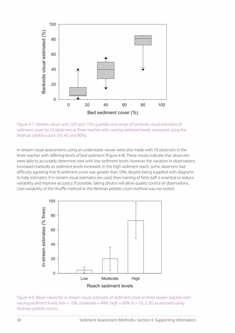
58 Sediment Assessment Methods • Section 4. Supporting information
Bed sediment cover (%)
0 20 40 60 80 100
Ban
ksid
e vi
sual
est
imat
ed (
%)
0
20
40
60
80
100
Figure 4-7. Median values and 25th and 75th quartiles and range of bankside visual estimates of sediment cover by 10 observers at three reaches with varying sediment levels measured using the Wolman pebble count (10, 40, and 80%).
In-stream visual assessments using an underwater viewer were also made with 10 observers in the three reaches with differing levels of bed sediment (Figure 4-8). These results indicate that observers were able to accurately determine sites with low sediment levels; however the variation in observations increased markedly as sediment levels increased. In the high sediment reach, some observers had difficulty agreeing that % sediment cover was greater than 50%, despite being supplied with diagrams to help estimates. If in-stream visual estimates are used, then training of field staff is essential to reduce variability and improve accuracy. If possible, taking photos will allow quality control of observations. User-variability of the Shuffle method or the Wolman pebble count method was not tested.
Reach sediment levels
Low Moderate High
In-s
trea
m e
stim
ates
(%
fine
s)
0
20
40
60
80
100
Figure 4-8. Mean values for in-stream visual estimates of sediment cover in three stream reaches with varying sediment levels: low = 10%, moderate = 40%, high = 80% (n = 10, ± SE) as assessed using Wolman pebble counts.

59Sediment Assessment Methods • Section 4. Supporting information
4.3.3 Do results vary in different land uses? Whether metric values differ between different land uses may reflect their sensitivity to anthropogenic pressure and/or natural environmental variation. For instance, small Waikato hill-country streams draining native forest had 2-3-fold lower SIS Quorer values than those draining pasture and pine forests (Quinn et al. 1997). SIS also tended to be higher in small Coromandel streams draining clear-cut pine plantations than non-harvested pine and native forest catchments and logged sites with continuous riparian buffers (Quinn et al. 2004).
To examine broad-scale spatial variability draft protocols were applied at 50 sites in the Canterbury region; predominantly first to third order streams on low gradient alluvial floodplains. Sites were grouped into five land-use and waterway categories: agricultural, urban, forest, spring-fed or mountain streams with 10 streams in each category. This was done in order to test potential variability in the protocols across both a gradient of sediment stress but also variable physical habitats.
Using the bankside visual protocols, some land uses and stream types had markedly higher levels of sediment than others (Figure 4-9). The agricultural and urban streams averaged 35-40% sediment. The forested streams of Banks Peninsula also had relatively high levels of sediment presumably due to ultrafine windblown loess soils that dominate these catchments, whereas spring-fed and mountain streams averaged about 20% sediment. The variation in % sediment (error bars) within each grouping of streams was similar among land uses, indicating that the protocols worked equally well under differing stream conditions.
Using Wolman pebble counts of % sediment, agricultural, urban and forested streams also showed relatively high % sediment, whereas spring-fed and mountain streams had lower % sediment consistent with the bankside visual estimates.
0
10
20
30
40
50
60
Agricultural Urban Forest Spring Mountain
Land use & stream types
Ba
nks
ide
vis
ua
l (%
se
dim
en
t)
0
10
20
30
40
50
60
70
Agricultural Urban Forest Spring Mountain
Land use & stream types
Wo
lma
n c
ou
nt (
% s
ed
ime
nt)
Figure 4-9. Mean % sediment for bankside visual and Wolman pebble counts in differing land uses and stream types in the Canterbury Plains (± 1SE, n = 10).
Comparisons of data from the Quorer and Shuffle methods showed slightly different results (Figure 4-10). The Quorer (using SIS values) showed urban streams had higher quantities of suspendible inorganic matter than the other four types of streams. The Quorer method differs from the bankside visual and Wolman method in that it measures the quantity of fine sediment on and within the upper layer of the streambed, rather than cover. The Shuffle method indicated that agricultural, urban and forested streams had higher amounts of bed sediment than spring-fed and mountain streams. The Shuffle method does not distinguish between organic and inorganic components of suspendible sediment, which may contribute to the different trend among land uses. The Shuffle results ranked stream types in a similar order as the bankside visual assessment – this suggests that protocols that do not distinguish between organic and inorganic components of sediment may result in similar spatial trends.

60 Sediment Assessment Methods • Section 4. Supporting information
0
1000
2000
3000
4000
5000
Agricultural Urban Forest Spring Mountain
Land use & stream types
Qu
ore
r S
IS (
g/m
2)
0
1
2
3
4
5
Agricultural Urban Forest Spring Mountain
Land use & stream types
Sh
uffl
e in
de
x
Figure 4-10. Mean values for Quorer SIS (g/m2) and Shuffle index scores in differing land uses and stream types in the Canterbury Plains (±1SE, n = 10).
4.3.4 How do results vary over time? The draft protocols were tested in one season (summer 2009/2010). However, historic datasets show that in-stream visual methods, Quorer SIS and Wolman pebble counts can be used to detect significant trends in sediment over time. Temporal trends in sediment may be caused by seasonal flow influences on the distribution of sediment, or pulses in sediment as a result of land use or natural disturbance events.
Datasets exist for Quorer and Wolman pebble counts from 11 years in the Whatawhata streams where SIS and % sediment, averaged across all sites, were 28% and 29% higher, respectively, in early autumn (March) than in spring (September) (Quinn et al. 2009). Both SIS and % sediment increased at a native forest stream after a tree fell into the reach and accumulated sediment upstream, demonstrating that these methods are able to detect changes due to natural influences even at relatively small scales. Percent sediment also showed a significant decrease in a small pasture stream following native forest riparian planting (Quinn et al. 2009).
Quorer derived SIS showed significant temporal patterns along the Tongariro River, a gravel-cobble bed river, in a one-year study of hydro-electricity generation related impacts on stream habitat and biota (Quinn & Vickers 1992) (Figure 4-11). SIS varied markedly with season and tended to be higher in winter and lower in spring, however this trend was strongly influenced by larger scale processes influencing the reach. This study indicates that SIS values at any site might fluctuate by 100% or more within a year.
In general, results from all methods detected differences in sediment values associated with different land uses. The similarity in variability among land uses suggests that the methods work similarly well in a range of stream settings.

61Sediment Assessment Methods • Section 4. Supporting information
Figure 4-11. Seasonal patterns of Quorer suspendible inorganic sediment (g/m2) in run habitat at sites down the Tongariro River in relation to the influences of sand input (from Rangipo Desert) and dams. Letters (above the bars) and lines (in seasons legend) indicate significant differences (p < 0.05) using two-way ANOVA with Bonferroni post-hoc multiple comparisons (adapted from Quinn & Vickers 1992).
Temporal variability has been observed over several years at sites throughout the Motueka River catchment using a method comparable to the in-stream visual assessment (L. Basher, pers. com.). A large flood in March 2005 mobilised sediment along the river resulting in greater than 20% of the bed having more than 50% sediment cover (Figure 4-12). Within six months, much of this sediment had been flushed from the site.
Figure 4-12. Temporal changes in % sediment cover in a run site on the Motueka River. A significant temporal trend was observed over a 5-yr period (p = 0.003). Data courtesy of Les Basher, Landcare Research.

62 Sediment Assessment Methods • Section 4. Supporting information
0.00.1
0.20.3
0.4
0.5
0.6
0.7
0.80.91.0
0 5 10 15 20 25 30
300 g/m2 change
400 g/m2 change
500 g/m2 change
Sample size
SIS g/m2 (median=356, SD=210)
Pow
er
Figure 4-13. The effect of sample size and the desired effect size on statistical power of comparisons of suspendible inorganic sediment (SIS) measurements.
A similar analysis can be conducted for the other protocols which involve replicate measures at a site. With 20 replicate measurements the proposed in-stream visual protocol should enable satisfactory statistical power to detect a change of 15% fine sediment cover at a site (Table 4-5). Similarly, the proposed Shuffle method involving three replicate measurements should enable satisfactory power to detect a change of one unit in the Shuffle index score.
4.3.5 How many replicates are required? The number of replicates required for a sampling programme depends on the expected variability among replicate measurements, the size of the effect, and the statistical power required to detect an effect of this size. Statistical power is maximised when there are a large number of replicate measurements, low variability among replicate measurements, and there is a large effect. Typically a statistical power of 0.8 is considered satisfactory – i.e., there is an 80% chance of detecting an effect of a certain size given the number of replicates and the variability among those replicates.
By examining the observed variability among replicate measurements for each of the protocols it is possible to give some guidance on the number of replicate samples required to detect an effect of a particular size. For example, using the average variability observed within sites for the protocol trials only three to four replicate measurements of suspendible sediment are required to have satisfactory statistical power to detect a 500 g/m2 change in suspendible sediment. However, six replicate measurements are required to have the same statistical power to detect a change of 400 g/m2 (Figure 4-13). The proposed protocol for suspendible sediment assessment which involves six replicate measurements (Section 2.3) will enable satisfactory power to detect a change in SIS of 400 g/m2.

63Sediment Assessment Methods • Section 4. Supporting information
Table 4-5. Summary of the number of replicates required for sediment protocols to confidently (power = 0.8) detect a range of effect sizes.
Protocol Size of effect to be detected
Number of replicates required to have satisfactory statistical power (0.8)
Suspendible sediment 300 g/m2
400 g/m2
500 g/m2
9
6
4
In-stream visual 10% change in cover
15% change in cover
25% change in cover
36
18
10
Shuffle 0.3 units
0.5 units
1 unit
26
10
3
Sediment depth 10 mm
20 mm
30 mm
50+
16
8
4.3.6 How do results from different protocols compare?Data from regional council trials were used to examine the correlations between data from different protocols, including bankside visual (Bankside), in-stream visual (In-stream), % sediment from Wolman pebble counts (Wolman), suspendible inorganic sediment (SIS), suspendible organic sediment (SOS), Shuffle index score (Shuffle) and sediment depth (Depth). Data were transformed to improve normality where necessary. The only protocol which did not compare well was sediment depth. Pearson correlation coefficients showed strong relationships between visual estimates of fine sediment cover, for example, bankside and in-stream visual r = 0.89, p < 0.01 (Figure 4-14). The Quorer metrics were also highly correlated, for example, log-SIS and log-SOS, r = 0.85, p < 0.001. The Shuffle index was significantly correlated with all other sediment measures, except sediment depth (Figure 4-14).
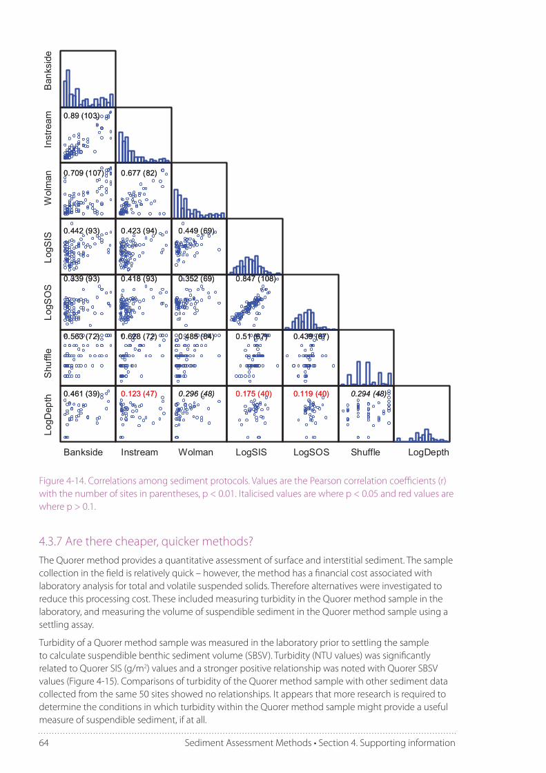
64 Sediment Assessment Methods • Section 4. Supporting information
RU
NV
ISU
ALA
VE
W2
LOG
SIS
LOG
SO
SS
CO
RE
RUN
LOG
DE
PT
H
VISUALAVE W2 LOGSIS LOGSOS SCORE LOGDEPTHBankside Instream Wolman LogSIS LogSOS Shuffle LogDepth
Log
Dep
thS
huffl
eL
ogS
OS
Log
SIS
Wol
man
Inst
ream
Ban
ksid
e
0.89 (103)
0.709 (107) 0.677 (82)
0.442 (93) 0.423 (94) 0.449 (69)
0.339 (93) 0.418 (93) 0.352 (69) 0.847 (108)
0.563 (72) 0.628 (72) 0.485 (84) 0.51 (67) 0.439 (67)
0.461 (39) 0.123 (47) 0.296 (48) 0.175 (40) 0.119 (40) 0.294 (48)
Figure 4-14. Correlations among sediment protocols. Values are the Pearson correlation coefficients (r) with the number of sites in parentheses, p < 0.01. Italicised values are where p < 0.05 and red values are where p > 0.1.
4.3.7 Are there cheaper, quicker methods? The Quorer method provides a quantitative assessment of surface and interstitial sediment. The sample collection in the field is relatively quick – however, the method has a financial cost associated with laboratory analysis for total and volatile suspended solids. Therefore alternatives were investigated to reduce this processing cost. These included measuring turbidity in the Quorer method sample in the laboratory, and measuring the volume of suspendible sediment in the Quorer method sample using a settling assay.
Turbidity of a Quorer method sample was measured in the laboratory prior to settling the sample to calculate suspendible benthic sediment volume (SBSV). Turbidity (NTU values) was significantly related to Quorer SIS (g/m2) values and a stronger positive relationship was noted with Quorer SBSV values (Figure 4-15). Comparisons of turbidity of the Quorer method sample with other sediment data collected from the same 50 sites showed no relationships. It appears that more research is required to determine the conditions in which turbidity within the Quorer method sample might provide a useful measure of suspendible sediment, if at all.

65Sediment Assessment Methods • Section 4. Supporting information
Turbidity (NTU)
SIS
(gm
2 )
r2 = 0.24P < 0.001
10,000
1,000
100
1
10 100 1000 10,000
Turbidity (NTU)
SB
SV
0.01
0.1
1
10
100
10 100 1,000 10,000
r2=0.76P<0.001
Figure 4-15. Comparison of metrics generated from Quorer method samples collected from 50 sites on the Canterbury Plains, including turbidity (NTU), suspendible inorganic sediment (g/m2) and suspendible benthic sediment volume (ml/m2). Note the log-scale of both axes.
Ninety-three Quorer method samples were processed to measure suspendible inorganic sediment (SIS) and suspendible benthic sediment volume (SBSV) using a settling assay. This assay involved letting the samples settle in a cylinder and measuring the volume of settled sediment. The values from these two methods were generally closely correlated for any given sample (Figure 4-16). A linear regression showed a significant positive relationship (r2 = 0.43, F (1, 48) = 35.79, p < 0.001) and results suggested that SBSV could provide a surrogate for SIS. An SIS value of 400 g/m2 is in the region of a SBSV value of 3000 ml/m2. However, the same method should be used for all samples which are going to be compared; this trial indicated that not all data points fall directly along the trend line and converting from one measure to the other will introduce some error.
Figure 4-16. Comparison of measurements of amounts of suspendible inorganic sediment (SIS) based on dry weights with areal suspendible benthic sediment volume from settled volumes for 93 samples (five outliers, with SIS >2000 g/m2, are not shown).
SIS (g/m2)
SB
SV
(m
L/m
2 )
0
2000
4000
6000
8000
10000
12000
14000
16000
0 200 400 600 800 1000 1200 1400 1600
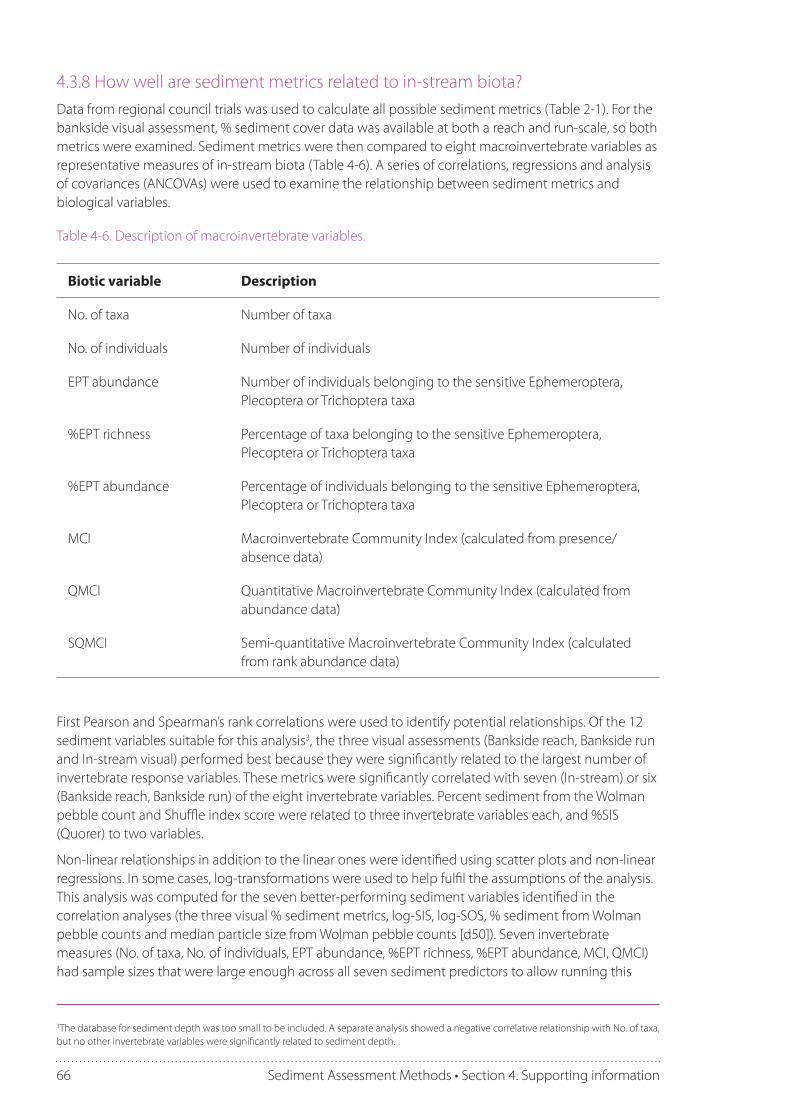
66 Sediment Assessment Methods • Section 4. Supporting information
4.3.8 How well are sediment metrics related to in-stream biota?Data from regional council trials was used to calculate all possible sediment metrics (Table 2-1). For the bankside visual assessment, % sediment cover data was available at both a reach and run-scale, so both metrics were examined. Sediment metrics were then compared to eight macroinvertebrate variables as representative measures of in-stream biota (Table 4-6). A series of correlations, regressions and analysis of covariances (ANCOVAs) were used to examine the relationship between sediment metrics and biological variables.
Table 4-6. Description of macroinvertebrate variables.
Biotic variable Description
No. of taxa Number of taxa
No. of individuals Number of individuals
EPT abundance Number of individuals belonging to the sensitive Ephemeroptera, Plecoptera or Trichoptera taxa
%EPT richness Percentage of taxa belonging to the sensitive Ephemeroptera, Plecoptera or Trichoptera taxa
%EPT abundance Percentage of individuals belonging to the sensitive Ephemeroptera, Plecoptera or Trichoptera taxa
MCI Macroinvertebrate Community Index (calculated from presence/absence data)
QMCI Quantitative Macroinvertebrate Community Index (calculated from abundance data)
SQMCI Semi-quantitative Macroinvertebrate Community Index (calculated from rank abundance data)
First Pearson and Spearman’s rank correlations were used to identify potential relationships. Of the 12 sediment variables suitable for this analysis3, the three visual assessments (Bankside reach, Bankside run and In-stream visual) performed best because they were significantly related to the largest number of invertebrate response variables. These metrics were significantly correlated with seven (In-stream) or six (Bankside reach, Bankside run) of the eight invertebrate variables. Percent sediment from the Wolman pebble count and Shuffle index score were related to three invertebrate variables each, and %SIS (Quorer) to two variables.
Non-linear relationships in addition to the linear ones were identified using scatter plots and non-linear regressions. In some cases, log-transformations were used to help fulfil the assumptions of the analysis. This analysis was computed for the seven better-performing sediment variables identified in the correlation analyses (the three visual % sediment metrics, log-SIS, log-SOS, % sediment from Wolman pebble counts and median particle size from Wolman pebble counts [d50]). Seven invertebrate measures (No. of taxa, No. of individuals, EPT abundance, %EPT richness, %EPT abundance, MCI, QMCI) had sample sizes that were large enough across all seven sediment predictors to allow running this
3The database for sediment depth was too small to be included. A separate analysis showed a negative correlative relationship with No. of taxa, but no other invertebrate variables were significantly related to sediment depth.

67Sediment Assessment Methods • Section 4. Supporting information
analysis. Once again, the three visual % sediment metrics performed best, and ‘Bankside reach’ was the top performer overall. It was significantly related to all key invertebrate metrics (r2 values ranged from 0.13-0.32); all five invertebrate metrics showing either linear or quadratic declines with increasing sediment. Log-SOS (Quorer) had the strongest relationship with MCI and QMCI (r2 = 0.24 in both cases) but was relevant for fewer invertebrate metrics than the % sediment measures. The relationship between Bankside reach and MCI had similar strength (r2 = 0.16). Percent sediment in Wolman counts and Shuffle index were both less relevant (in terms of the number of invertebrate metrics affected and also the r2 values of these relationships). The generally fairly low r2-values for these relationships indicate that several other factors influenced the investigated invertebrate response variables besides the amount of deposited fine sediment at the study sites. The potential roles of two of these additional factors were examined in our next analysis.
Finally, the influence of region and stream size in the relationships between six sediment metrics (three % sediment metrics, log-SIS, log SOS and % sediment in Wolman pebble counts) and MCI and %EPT richness was investigated. Adding ‘region’ as a predictor had a significant effect for all six sediment variables and increased the r2-values of the linear models to a precision (26-54% of the variation in the data explained) that is fairly high for ecological survey data. In every single case, the effect size for region (range 0.17-0.38; effect sizes can theoretically range from 0.0 to 1.0) was greater than the effect size of the sediment predictor in question (range 0.05-0.18). Nevertheless, all three visual % sediment metrics (and also Wolman % sediment, but neither SIS nor SOS) were still significantly and negatively correlated with MCI and %EPT. Based on their effect sizes, In-stream visual and Bankside reach were the best sediment predictors for MCI, and Wolman % sediment and In-stream were the best predictors for %EPT richness. In conclusion, regional variation and/or variation between different operators played an important role in this study as expected, but this variation had relative little effect on the main conclusions drawn from the previous analyses.
In practise, differences between geographical regions should not be a major problem for determining sediment-invertebrate relationships during future biomonitoring in New Zealand because regional councils usually collect all their data within a single geographical region. However, because the factor ‘region’ also included potential differences between different operators, training all operators using standardised criteria to minimise between-operator variation in all assessments of sediment is recommended.
Adding ‘stream size’ (using stream width and depth data) as a covariate had no significant effect: p = 0.11 for Wolman % sediment and MCI, and p > 0.29 in all other cases. The results indicated that the observed relationships between the six sediment predictors and MCI or %EPT were independent of stream size.
4.3.9 Other useful things discovered along the wayBankside visual estimate
Can I stand in one place to make an assessment (e.g., on a bridge)?
The bankside visual assessment should take into account the full sample reach. Usually, it is necessary to walk along the river bank (sometimes both sides in larger rivers) to estimate sediment cover for the full sample habitat. Bankside reach-scale and run-scale assessments of % cover are highly correlated, but analyses show a stronger relationship between run-scale assessments and in-stream values.
In-stream visual estimate
Do I need to record a measurement for every quadrant on the viewer?
Quadrants are very useful for training purposes and quality control among users. Once a user ‘has their eye in’ it is not necessary to record data for every quadrant.

68 Sediment Assessment Methods • Section 4. Supporting information
Limitations with the bathyscope
The scope can be difficult to use in shaded areas where the stream bed is hard to see. It is difficult to use in faster water and if you have shallow, fast water the scope can cause turbulence which will entrain sediment, altering your readings.
Wolman pebble count
To work well this needs the observer to take care in randomly selecting particles and ensuring that they record fine sediment among larger particles.
Quorer method
How long do I stir the sediment before collecting a sample?
A small experiment was conducted where samples were collected after 15, 30, 45 and 60 seconds of stirring. Results (Figure 4-17) suggested that 15 seconds was ample to provide an accurate measure of SIS.
Time (sec)
Tur
bidi
ty (
NT
U)
0
500
1000
1500
2000
2500
15 30 45 60
Figure 4-17. Relationship between turbidity and time of stirring in a Quorer sampler. N = 18.
Are there any physical limitations to applying the Quorer method?
The Quorer method is limited to locations where a corer can be deployed to form a tight seal on the streambed (influenced by streambed roughness, substrate size and current velocity) without the stream water over-topping into the cylinder (influenced by depth). In general, the method is limited to depths and velocities below approximately 0.5 m and 0.5 m/s, respectively, and substrate sizes up to gravel/cobble (not boulders). These limitations can be met to some extent by increasing the Quorer diameter (to deal with cobble/gravel beds) and depth. Large Quorers have been used with success by NIWA and Tasman District Council scientists (Figure 4-18). A metal Quorer method sampler with handles can be useful.

69Sediment Assessment Methods • Section 4. Supporting information
Figure 4-18. Large corers successfully applied to extend the physical limitations of the Quorer method.
Shuffle method
Both water depth and flow appear to bias this protocol when assigning scores based on views of a white tile. Possible refinements include using a pilot measure to inform the assessor as to which way the flow is going and where to place the tile, attaching the white tile to a pole and ensuring readings are made at 200 mm depth. The categorical nature of the index could be refined in future to a continuous variable which takes into account both flow and depth; by measuring the depth of the plume in relation to a white pole and the time it takes for the sediment plume to reach and subsequently clear the tile. However, it would be difficult to take into account the horizontal dispersion of the plume in the water column. Another possible approach involves reading the effect of standard bed disturbance in horizontal clarity with a water sample from the Quorer method measured in a mini Stream Health Monitoring and Assessment Kit (SHMAK) clarity tube. There are currently no data to validate this approach, but see Section 4.3.7 for discussion on surrogate measures.
Sediment depth
Limited data and weak relationships observed during protocols development suggested sediment depth is not a very sensitive indicator of sediment effects on biota (however, guideline development analyses indicated a relationship with taxa richness – see Section 4.5.3). Sediment depth might be a valuable measure for effects-based assessments. Measuring sediment depth in pools may also provide a more sensitive measure, but this was not tested in these trials.

70 Sediment Assessment Methods • Section 4. Supporting information
4.4 Review of existing guidelines4.4.1 New ZealandEnvironment Canterbury is the only Regional Council to currently provide numerical guidelines and include numerical objectives for the areal coverage of fine sediments within a spatial framework for the region (Environment Canterbury 2011, see Hayward et al. 2009 for rationale). Objectives range from 10% to 40% cover depending on the surface water ‘management unit’ of interest. These objectives have been calculated from data collected at 144 sites measured since 1999.
There are currently no national standards or guidelines to assess the effects of sediment on in-stream values in New Zealand.
4.4.2 InternationalMany river-type specific guidelines have been developed for areas of the United States and Canada (Table 4-7). To summarise, the most common sediment criteria in northern America are for the percent of sediment calculated from pebble counts or by mass and substrate embeddedness assessed using the USEPA qualitative method. Unfortunately recommended values for each state and province are difficult to interpret because of inconsistencies in the definition of fine sediment, i.e., anything from 0.64 mm to 6.4 mm.
4.5 Guideline developmentAn essential criterion for any guideline is that it must relate to a demonstrable effect that can be quantified (Jones et al. 2011). Thus manipulative experiments (laboratory and field-scale experiments) are often used to identify chronic and acute concentrations of contaminants (Table 4-8). There are examples of manipulative experiments in New Zealand that have identified biotic responses to sediment additions, although none specifically tested sediment thresholds (e.g., Ryder 1989; Dunning 1998; Suren & Jowett 2001; Matthaei et al. 2006; but see also Wagenhoff 2011). Decreases in mayfly, stonefly and caddisfly richness have been associated with increases in sediment cover (Table 4-1). Notably, Townsend et al. (2008) observed a decrease in EPT richness associated with higher sediment levels in a survey of 32 streams, whereas the response of EPT to experimental sediment and nutrient addition in nine agricultural streams was more complex.
More commonly, correlations with field survey data are used to develop sediment guidelines (Sutherland et al. 2008). While surveys do not provide proof of cause and effect and can be confounded by multiple stressor effects, they do identify sediment levels associated with changes in in-stream values.

71Sediment Assessment Methods • Section 4. Supporting information
Location Performance criteria Standard (target)
Alaska % fine sediment(0.1 mm – 4.0 mm by mass)
≤ 5% above reference or ≤ 30% absolute
Arizona % sediment in riffles (Wolman) ≤ 35%
British Columbia
% fine sediment in redds (by mass)Geometric mean diameter
≤ 10% (<2 mm) or≤ 25% (<6.35 mm)≥ 12 mm
California Geometric mean diameter% embeddedness in riffles% fine sediment in redds (by wet mass)
> 69 mm≤ 25%≤ 14% (<0.85 mm) or≤ 30% (<6.4 mm)
Colorado % sediment (Wolman)
% embeddedness
90-100% of expected condition = fully supporting73-89% of expected condition = partially supporting90-100% of expected condition = fully supporting73-89% of expected condition = partially supporting
Hawaii Fine sediment depth in hard-bottom streams
≤ 5 mm
Idaho % fine sediment in riffles (by mass)Riffle stability index (RSI)
≤ 10% (<0.85 mm)
≤ 70 RSI
Montana % fine sediment in riffles (by mass) ≤ 30% (<6.35 mm)
New Brunswick
% sediment (Wolman + visual estimate)Median particle size% sediment in riffles (by mass)
≤ 7.2% (<2 mm)≤ 9.3% (<6.35 mm)> 56.9 mm≤ 3% (<2 mm)
New Mexico % embeddedness ≤ 33% = fully supporting> 33% is compared to reference
% sediment in riffles (Wolman) < 20% = fully supporting> 20% compared to reference
Oregon % fine sediment in riffles (by mass) < 20%
Prince Edward Island
% sediment (Wolman + visual estimate)Median particle sizeRelative bed stability (RBS)
≤ 12.9% (<2 mm)≤ 12.7% (<6.35 mm)> 47.4 mm≤ 3.8 RBS
Table 4-7. Sediment criteria and standards for the United States and Canada (from Sutherland et al. 2008 and Culp et al. 2009)

72 Sediment Assessment Methods • Section 4. Supporting information
Table 4-8. Summary of approaches used to define sediment criteria summarised from Jones et al. (2011).
Guideline approach Advantages Disadvantages
Laboratory assessments Controlled
Definition of mortality limits
Individual response observable
Limited to target organisms/populations
Limited treatment options
Difficult to scale to stream
Field-scale experimental manipulations
(experimental channels and simulated events)
Similar to natural conditions
Population and community level response observable
Limited treatment options
High logistical requirements
Case studies of pollution events
Population through to ecosystem response observable
Logistically difficult
Requires opportunistic sampling often results in lack of ‘before’ data
Difficult to discern sediment effect versus other/background effect
Correlation with field survey data
Natural conditions and results relevant at management scale
Effects in the presence of multiple pressures observable
Population through to ecosystem response observable
Does not provide proof of cause and effect
Separating effects of co-variables (natural variability) is difficult
4.5.1 Sources of dataAn historic dataset was combined with data collected from our research to provide sediment information for 454 sites. Sites ranged from first to seventh order streams and had a wide spatial coverage – from Northland to Southland and all regions in between, except the West Coast. Classifying sites by stream type showed that five of the 20 FENZ 20-level groups were represented by the data (Groups A, C, D, G, H; for a description of stream types see Leathwick et al. 2011), but these five groups account for 83% of the national river network (Leathwick et al. 2011).

73Sediment Assessment Methods • Section 4. Supporting information
4.5.2 Correlation among sediment and biotaInitially, sediment measures were compared with each other. Variables were transformed where necessary to improve the normality of data distributions.
Correlation analyses identified similarity among all sediment measures (Figure 4-19). All three visual assessments of % cover (Bankside reach, Bankside run, In-stream visual) were strongly related (r > 0.85). Quorer measures (log-SIS, log-SOS) were significantly related to each other (r = 0.86, p < 0.01) and to bankside and in-stream visual assessments of % sediment cover at the run-scale (r = 0.42, p < 0.01), but not the reach-scale measure. The Shuffle index and Wolman measure of % sediment were significantly related to all metric measures (r > 0.40), except log-sediment depth. Sediment depth was only significantly related to five other metrics and the strongest of these relationships was with log-SOS (r = 0.48).
% fines Bankside
Reach visual
% finesBanksideRun visual
% finesIn-stream
visual
% finesWolman
LogSIS LogSOS Shuffle indexscore
LogDepth
% fi
nes
Ba
nksi
deR
un v
isua
l
% fi
nes
In-s
tre
amvi
sual
% f
ine
sW
olm
an
Log
SIS
LogS
OS
Sh
uffle
inde
xsc
ore
Log
De
pth
0.86 (125)
0.92 (84)
0.80 (90)
0.28 (86)
0.33 (85)
0.67 (52)
0.45 (32)
0.85 (167)
0.70 (171)
0.44 (186)
0.44 (186)
0.49 (134)
0.37 (98)
0.68 (146)
0.47 (206)
0.42 (206)
0.45 (134)
0.35 (153)
0.43 (232)
0.44 (233)
0.40 (146)
0.25 (107)
0.86 (355)
0.43 (125)
0.46 (142)
0.44 (126)
0.48 (143) 0.39 (105)
% fines Bankside
Reach visual
% finesBanksideRun visual
% fines
visual
% fines LogSIS LogSOS
0.80 (90)
0.28 (86)
0.33 (85)
0.67 (52)
0.45 (32)
0.85 (167)
0.70 (171)
0.44 (186)
0.44 (186)
0.49 (134)
0.37 (98)
0.68 (146)
0.47 (206)
0.42 (206)
0.45 (134)
0.35 (153)
0.43 (232)
0.44 (233)
0.40 (146)
0.25 (107)
0.86 (355)
0.43 (125)
0.46 (142)
0.44 (126)
0.48 (143) 0.39 (105)
% fines Bankside
Reach visual
% finesBanksideRun visual
% finesIn-stream
visual
% finesWolman
LogSIS LogSOS Shuffle indexscore
LogDepth
% fi
nes
Ba
nksi
deR
un v
isua
l
% fi
nes
In-s
tre
amvi
sual
% f
ine
sW
olm
an
Log
SIS
LogS
OS
Sh
uffle
inde
xsc
ore
Log
De
pth
0.86 (125)
0.92 (84)
0.80 (90)
0.28 (86)
0.33 (85)
0.67 (52)
0.45 (32)
0.85 (167)
0.70 (171)
0.44 (186)
0.44 (186)
0.49 (134)
0.37 (98)
0.68 (146)
0.47 (206)
0.42 (206)
0.45 (134)
0.35 (153)
0.43 (232)
0.44 (233)
0.40 (146)
0.25 (107)
0.86 (355)
0.43 (125)
0.46 (142)
0.44 (126)
0.48 (143) 0.39 (105)
% fines Bankside
Reach visual
% finesBanksideRun visual
% fines
visual
% fines LogSIS LogSOS
0.80 (90)
0.28 (86)
0.33 (85)
0.67 (52)
0.45 (32)
0.85 (167)
0.70 (171)
0.44 (186)
0.44 (186)
0.49 (134)
0.37 (98)
0.68 (146)
0.47 (206)
0.42 (206)
0.45 (134)
0.35 (153)
0.43 (232)
0.44 (233)
0.40 (146)
0.25 (107)
0.86 (355)
0.43 (125)
0.46 (142)
0.44 (126)
0.48 (143) 0.39 (105)
Figure 4-19. Correlations among metrics from data collated for guideline development. Values are the Pearson correlation coefficient (r) with number of sites in parentheses, p < 0.01. Red values are where p > 0.1. Note log10 transformations of SIS, SOS and sediment depth data.

74 Sediment Assessment Methods • Section 4. Supporting information
Sediment data was then compared in relation to biotic metrics representing in-stream values: MCI, %EPT richness, taxonomic richness, EPT taxa richness, % trout, % native fish, koura abundance, and eel abundance. There were no significant relationships between the Shuffle index score and any of the values metrics. There were also no significant correlations between any of the sediment measures and fish metrics; however, both MCI and %EPT richness were related to sediment metrics. Log-sediment depth had a significant relationship with the number of invertebrate taxa and the number of EPT taxa (Figure 4-20).
-0.45 (124) -0.37 (141)
% fines Bankside Reach visual
MC
I
% fines Bankside Run visual
MC
I
% fines In-stream visual
MC
I
LogSIS
MC
I
-0.38 (168)-0.40 (183)
% fines Bankside reach visual
% E
PT
ric
hnes
s
% fines Bankside Run visual
% E
PT
ric
hnes
s
% fines Instream visual
% E
PT
ric
hnes
s
% fines Wolman
% E
PT
ric
hnes
s
-0.56 (126) -0.43 (143) -0.47 (113)
-0.42 (120)
LogSOS
MC
I
LogDepth
No.
tax
a-0.48 (154)
-0.38 (93)
LogDepth
No.
EP
T t
axa
-0.52 (77)
-0.45 (124) -0.37 (141)
% fines Bankside Reach visual % fines Bankside Run visual
LogSIS
MC
I
-0.38 (168)-0.40 (183)
% fines Bankside reach visual
% E
PT
ric
hnes
s
% fines Wolman
% E
PT
ric
hnes
s
-0.56 (126) -0.43 (143) -0.47 (113)
-0.42 (120)
LogSOS
MC
I
LogDepth
No.
tax
a-0.48 (154)
-0.38 (93)
LogDepth
taxa
-0.52 (77)
-0.45 (124) -0.37 (141)
% fines Bankside Reach visual
MC
I
% fines Bankside Run visual
MC
I
% fines In-stream visual
MC
I
LogSIS
MC
I
-0.38 (168)-0.40 (183)
% fines Bankside reach visual
% E
PT
ric
hnes
s
% fines Bankside Run visual
% E
PT
ric
hnes
s
% fines Instream visual
% E
PT
ric
hnes
s
% fines Wolman
% E
PT
ric
hnes
s
-0.56 (126) -0.43 (143) -0.47 (113)
-0.42 (120)
LogSOS
MC
I
LogDepth
No.
tax
a-0.48 (154)
-0.38 (93)
LogDepth
No.
EP
T t
axa
-0.52 (77)
-0.45 (124) -0.37 (141)
% fines Bankside Reach visual % fines Bankside Run visual
LogSIS
MC
I
-0.38 (168)-0.40 (183)
% fines Bankside reach visual
% E
PT
ric
hnes
s
% fines Wolman
% E
PT
ric
hnes
s
-0.56 (126) -0.43 (143) -0.47 (113)
-0.42 (120)
LogSOS
MC
I
LogDepth
No.
tax
a-0.48 (154)
-0.38 (93)
LogDepth
taxa
-0.52 (77)
Figure 4-20. Correlations among sediment measures and metrics of in-stream values. Values are the Pearson correlation coefficient (r) with number of sites in parentheses. Only significant relationships (p < 0.01) are shown.

75Sediment Assessment Methods • Section 4. Supporting information
4.5.3 Predictive relationships between sediment and biotaBased on the results of correlation analyses, the strength of relationships between biotic indices and sediment metrics was investigated using linear regression of the combined data set.
1. Percent sediment and MCI and %EPT richness
The strongest relationship observed between MCI and % sediment was for the reach scale bankside measure: r2 = 0.20, p < 0.001 (Figure 4-21). Using the linear relationship (y=113.19-0.29x) to predict the sediment value at 120 MCI (i.e., the value separating clean waters from possible pollution) leads to a theoretical value of -23% sediment cover, i.e., an absence of sediment. Also, it is apparent from Figure 4-21 that there is a large spread of MCI values at 0% sediment cover, anywhere between 90 and 142 MCI, probably reflecting the effects of factors other than % sediment on MCI. Clearly a regression approach is not a meaningful or sensitive way to assign guideline values.
The bankside reach scale estimate of % sediment had the strongest relationship with %EPT richness: r2 = 0.32, p < 0.001 (Figure 4-21). Using the linear relationship (y=52.49-0.33x) to predict sediment cover at a %EPT value indicative of clean water (50% EPT) results in sediment cover value of 7%. However, there was a wide range of %EPT values at less than 7% sediment; 7% EPT – 90% EPT.
0 20 40 60 80 100
Bankside reach (% sediment)
0
60
120
180
MC
I
0 20 40 60 80 100
Bankside reach (% sediment)
0
60
120
180
MC
I
0 20 40 60 80 100
Bankside reach (% sediment)
0
20
40
60
80
100
%E
PT
ric
hnes
s
0 20 40 60 80 100
Bankside reach (% sediment)
0
20
40
60
80
100
%E
PT
ric
hnes
s
Figure 4-21. Linear relationship (with 95% prediction confidence intervals) between a reach scale bankside estimate of % fine sediment cover and the MCI metric (n = 124), and %EPT richness (n = 126). The blue line indicates the % fine sediment value where %EPT exceeds 50%.
2. Suspendible sediment and MCI
The relationship between measures of organic and inorganic suspendible sediment and MCI was examined. There were relatively weak yet significant linear relationships with MCI for log-transformed SOS: r2 = 0.26, p < 0.001 and log-transformed SIS: r2 = 0.18, p < 0.001 (Figure 4-22). Using the linear relationship (y=125.90-13.93x) to predict the log-SOS value at 120 MCI (i.e., clean water) results in a value of 0.42, equivalent to a back-transformed value of 2.65 g/m2. Similarly, for log-SIS the predicted value at 120 MCI based on the linear relationship (y=135.62-11.67x) was 1.34, equivalent to a back-transformed value of 21.8 g/m2.
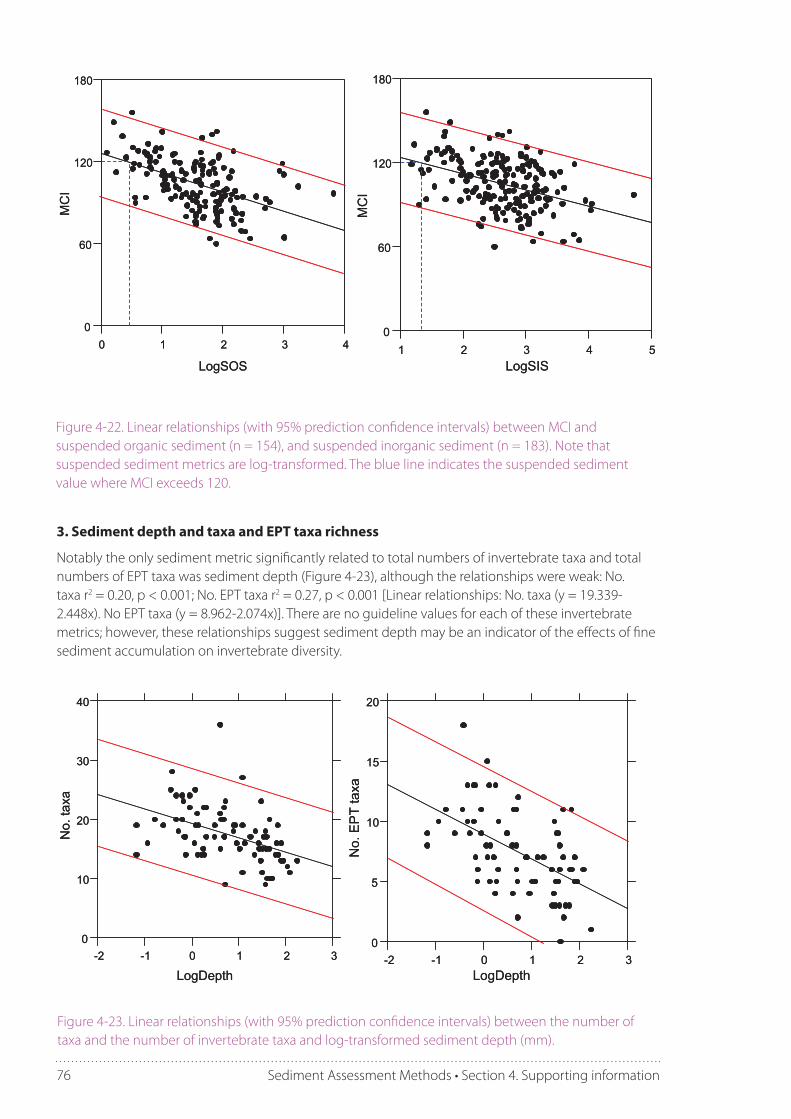
76 Sediment Assessment Methods • Section 4. Supporting information
0 1 2 3 4
LogSOS
0
60
120
180
MCI
0 1 2 3 4
LogSOS
0
60
120
180
MCI
1 2 3 4 5
LogSIS
0
60
120
180
MCI
1 2 3 4 5
LogSIS
0
60
120
180
MCI
Figure 4-22. Linear relationships (with 95% prediction confidence intervals) between MCI and suspended organic sediment (n = 154), and suspended inorganic sediment (n = 183). Note that suspended sediment metrics are log-transformed. The blue line indicates the suspended sediment value where MCI exceeds 120.
3. Sediment depth and taxa and EPT taxa richness
Notably the only sediment metric significantly related to total numbers of invertebrate taxa and total numbers of EPT taxa was sediment depth (Figure 4-23), although the relationships were weak: No. taxa r2 = 0.20, p < 0.001; No. EPT taxa r2 = 0.27, p < 0.001 [Linear relationships: No. taxa (y = 19.339-2.448x). No EPT taxa (y = 8.962-2.074x)]. There are no guideline values for each of these invertebrate metrics; however, these relationships suggest sediment depth may be an indicator of the effects of fine sediment accumulation on invertebrate diversity.
-2 -1 0 1 2 3
LogDepth
0
10
20
30
40
No.
taxa
-2 -1 0 1 2 3
LogDepth
0
10
20
30
40
No.
taxa
-2 -1 0 1 2 3
LogDepth
0
5
10
15
20
No.
EP
T ta
xa
-2 -1 0 1 2 3LogDepth
0
5
10
15
20
No.
EP
T ta
xa
Figure 4-23. Linear relationships (with 95% prediction confidence intervals) between the number of taxa and the number of invertebrate taxa and log-transformed sediment depth (mm).

77Sediment Assessment Methods • Section 4. Supporting information
4.5.4 Boosted regression tree model to inform reference stateAn output of a parallel research project (MSI contract C01X1005) was the development of a regression model that determines the relationship between fine sediment cover and environmental predictors. This model was then used to predict the relative proportion of fine sediment cover in every stream reach in New Zealand (see Appendix 6.3 for model details). Sediment data used in model development was sourced from the Freshwater Fisheries database. The % fine sediment cover was calculated from a bankside estimate of the relative proportion of substrate size classes. Environmental variables were sourced from the FENZ database and included measures of land use, climate, geology, morphology and topography as described in Leathwick et al. (2011). The resulting boosted regression tree model had a cross-validation error of 0.67 and explained 45% of the variance in % fine sediment cover (n = 10,026), which indicate good model performance. The fitted functions of explanatory variables were as expected with fine sediment cover increasing in response to decreasing upstream average slope and segment slope, decreasing native vegetation cover in the catchment, segment flow and flow stability. Sediment cover increased in response to increasing mean air summer and temperature annual variability and land-use intensification. Fitted functions from the model were used to predict fine sediment cover in each NZREACH stream segment in New Zealand (Figure 4-24). Predicted fine sediment cover values ranged from 0% to 100% and the national average value was 29.4%.

78 Sediment Assessment Methods • Section 4. Supporting information
Figure 4-24. Predicted contemporary sediment cover for stream segments in the New Zealand river network. For more information on the source model see Appendix 6.3.

79Sediment Assessment Methods • Section 4. Supporting information
Figure 4-25. Predicted reference* values for fine sediment cover in the New Zealand river network. *Reference is defined by the absence of human land-use impacts. For more information on the source model see Appendix 6.3.

80 Sediment Assessment Methods • Section 4. Supporting information
Next, the effect of land-use variables (native vegetation cover, impervious surface cover and predicted nitrogen concentrations as an indicator of land-use intensity) were fixed and used as an offset in a model to predict fine sediment cover in the absence of land use. The resulting boosted regression tree model had a cross-validation error of 0.63 and explained 42% of the variance in the sediment data. The small decrease in model performance compared to the former inclusive model provides confidence in the fixed model output. The fitted functions from this second model were used to predict sediment cover for each NZREACH based solely on environmental variability, i.e., expected ‘reference’ values in the absence of land use (Figure 4-25). As expected, from the fitted functions of the former model, high levels of fine sediment cover were predicted for areas of relatively low slope, high temperature and low rainfall, low flow and soft geology, for example, Northland, coastal Bay of Plenty, coastal Manawatu and Hawkes Bay, and plateau areas of upland Otago.
Predicted reference values for fine sediment cover in New Zealand streams ranged from 0% to 100% with an average value of 7.7%. A summary of modelled contemporary and modelled reference values for sediment cover in each stream segment based on FENZ 20-level groupings further illustrates the logical output of the model predictions (Table 4-9). As expected, small coastal to inland streams with low gradient and low rain days had the highest predicted sediment cover (Groups A-D, F & G); but these streams have also been subject to the highest land-use pressure and hence have the largest divergence between predicted contemporary and predicted reference values.
Independent values from the protocol development phase were used to validate the model predictions. The strongest correlation was between the bankside reach scale estimate of sediment cover and the modelled observed measure: r = 0.58, p < 0.001 (Figure 4-26). The relationship with all other estimates of % sediment were significant (p < 0.001), but not as strong: Bankside run, r = 0.40, n = 244; In-stream visual, r = 0.29, n = 236; Wolman r = 0.42, n = 291).
The validation is good and the correlation is almost as strong as the predictive error of the model (CV = 0.63). However, it is clear from Figure 4-26 that the model has the potential to both over- and under-estimate sediment cover at both the high and low ends of the range in values. The linear relationship suggests the predictive model is likely to overestimate low sediment cover and underestimate high sediment cover.

81Sediment Assessment Methods • Section 4. Supporting information
Table 4-9. Fine sediment spatial model predictions of contemporary values (O), reference values (E) and the 75th percentile value at sites with greater than 80% vegetation (O80) summarised by FENZ 20-level grouping. Mean values are shown for each FENZ group.
FENZ Group O E O80
A 67.52 16.14 57.84
B 74.90 29.45 77.62
C 23.90 5.85 9.66
D 33.41 5.70 8.48
E 23.56 16.43 29.41
F 45.72 23.21 44.40
G 25.21 6.71 15.29
H 8.73 4.19 8.42
I 9.64 7.59 12.65
J 4.42 2.55 5.56
K 3.19 2.79 4.87
L 2.31 1.96 3.03
M 7.07 5.98 11.10
N 7.48 5.75 10.10
O 4.57 3.46 5.94
P 5.45 4.72 7.20
Q 4.88 4.06 6.27
R 8.16 8.14 5.64
S 2.59 2.44 3.25
T 3.37 3.34 4.10

82 Sediment Assessment Methods • Section 4. Supporting information
0 20 40 60 80 100
% fines (model predictions)
0
20
40
60
80
100
% fi
nes
(Ban
ksid
ere
ach)
Figure 4-26. Correlation between % fine sediment estimated from the bankside reach measure and predictions from the spatial model (n = 130).
4.5.5 Data mining to inform reference stateExpected sediment values for minimally impacted sites (‘reference’) were defined by examining the distribution of data collated to develop guidelines by using sites:
1. characterised by greater than 80% native vegetation cover in the catchment,
2. where MCI values were >120 (i.e., clean water, Boothroyd & Stark 2000), and
3. where %EPT values were >50.
For example, using this approach the % fine sediment cover measured using the bankside visual method (at a run scale) suggests two alternative reference values, the 75th percentile at greater than 80% native vegetation cover is 15% and the 75th percentile at greater than 120 MCI and 50 %EPT is 20% (Figure 4-27). The reference values were very similar for determinations based on greater than 80% native vegetation cover (Table 4-10) and >120 MCI (Table 4-11) and >50 %EPT (Table 4-12) for most metrics.

83Sediment Assessment Methods • Section 4. Supporting information
0 20 40 60 80 100
0 20 40 60 80 100
Sites with >80% native vegetation, N = 19
Sites with >120 MCI,N = 29
75th percentile = 15%
75th percentile = 20%
0 20 40 60 80 100
0 20 40 60 80 100
Sites with >80% native vegetation, N = 19
Sites with >120 MCI,N = 29
75th percentile = 15%
75th percentile = 20%
0 20 40 60 80 100
% fine sediment
Sites with >50% EPT,N = 45
75th percentile = 20%
0 20 40 60 80 100
% fine sediment
75th percentile = 20%
0 20 40 60 80 100
0 20 40 60 80 100
Sites with >80% native vegetation, N = 19
Sites with >120 MCI,N = 29
75th percentile = 15%
75th percentile = 20%
0 20 40 60 80 100
0 20 40 60 80 100
Sites with >80% native vegetation, N = 19
Sites with >120 MCI,N = 29
75th percentile = 15%
75th percentile = 20%
0 20 40 60 80 100
% fine sediment
Sites with >50% EPT,N = 45
75th percentile = 20%
0 20 40 60 80 100
% fine sediment
75th percentile = 20%
Figure 4-27. Example of using data distributions to calculate guideline values for % fine sediment cover estimated using the bankside reach protocol.
Table 4-10. The 75th percentile for sediment metrics at sites with greater than 80% native vegetation cover in their catchments.
Site with greater than 80% native vegetation N 75th percentile
% sediment (Bankside reach) 19 15.00
% sediment (Bankside run) 37 20.00
% sediment (In-stream visual) 36 17.02
% sediment (Wolman) 58 17.50
SIS (g/m2) 74 404.53
SOS (g/m2) 69 28.20
%SIS 69 91
Shuffle index score 24 2.15
Sediment depth (mm) 23 8.87

84 Sediment Assessment Methods • Section 4. Supporting information
Sites with greater than 120 MCI N 75th percentile
% sediment (Bankside reach) 29 20.00
% sediment (Bankside run) 35 20.00
% sediment (In-stream visual) 36 13.02
% sediment (Wolman) 20 8.00
SIS (g/m2) 41 429.28
SOS (g/m2) 33 43.47
%SIS 33 94
Shuffle index score 14 2.00
Sediment depth (mm) 15 4.10
Sites with greater than 50 %EPT N 75th percentile
% sediment (Bankside reach) 45 20.00
% sediment (Bankside run) 56 20.00
% sediment (In-stream visual) 48 16.60
% sediment (Wolman) 39 20.50
SIS (g/m2) 48 952.72
SOS (g/m2) 48 69.39
%SIS 48 94
Shuffle index score 35 3.00
Sediment depth (mm) 12 62.69
Table 4-11. The 75th percentile for sediment metrics at sites with >120 MCI.
Table 4-12. The 75th percentile for sediment metrics at sites with >50 %EPT.
4.5.6 Amenity valuesA functional approach to defining benchmarks is often used when values other than aquatic life are of interest. For example, visual clarity guidelines are an example of a ‘functional benchmark’ to protect recreational use: ‘The visual clarity guidelines are based on the objective that to protect visual clarity of waters used for swimming, the horizontal sighting of a 200 mm diameter black disc should exceed 1.6 m (ANZECC 2000). Functional benchmarks can be determined by results from the literature, field data or social data, for example, surveys.
A survey was conducted to determine what levels of sediment are socially acceptable for swimming and to determine the levels of sediment that affect the aesthetic values of streams. Participants of a

85Sediment Assessment Methods • Section 4. Supporting information
sediment workshop at the New Zealand Freshwater Science Society annual conference (Christchurch, November 2010) were asked to complete a survey (Appendix 6.2). The survey contained a series of photos and participants4 were asked to provide good/bad or yes/no responses to the following questions:
1. Focussing on the level of fine sediment, how do you feel (gut feeling) about this stream?
2. In your opinion, is this level of fine sediment acceptable for swimming?
Results were used to determine a range in sediment values that were indicative of a change in aesthetic and swimming values of streams. Based on 48 responses to the first question, amenity value changes from acceptable to unacceptable between 12% and 27.5% sediment cover (Table 4-13). Based on 48 responses to the second question, swimming value decreases from acceptable to unacceptable between a Shuffle index score of 2 and a Shuffle index score of 3 (Table 4-14).
4A recognised biased sample of people who are likely to make informed decisions based on their professional experience in freshwater. Of the 48 respondents, 62% were male; the average age was 39 years (range 24-65 yrs) with an average number of 13 years (range 1-40 yrs) of professional experience in freshwater.
Table 4-13. Summary of responses to Question one from the Amenity Values Survey, “Focussing on the level of fine sediment, how do you feel (gut feeling) about this stream?” Survey results are the percentage of responses where green indicates an answer of “Good” and orange “Bad”.
% sediment
Survey photo Survey results Overall rating
2.5%
81.2%
18.7%
81.2%
18.7%
Good
5%
93.7%
6.2%
93.7%
6.2%
Good
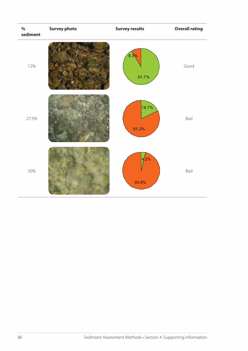
86 Sediment Assessment Methods • Section 4. Supporting information
% sediment
Survey photo Survey results Overall rating
12%
91.7%
8.3%
91.7%
8.3%
Good
27.5%
18.7%
81.2%
18.7%
81.2%
Bad
50%
4.2%
95.8%
4.2%
95.8%
Bad

87Sediment Assessment Methods • Section 4. Supporting information
Table 4-14. Summary of responses to Question two from the Amenity Values Survey, “In your opinion, is this level of fine sediment acceptable for swimming?” Survey results are the percentage of responses where green indicates an answer of “Yes” and orange “No”.
Shuffle Survey photo Survey results Overall rating
1
Yes
2
93.7%
6.2%
93.7%
6.2%
Yes
3 No
4 No
5 No
96%
4%
96%
4%
6%
94%
6%
94%
12%
88%
12%
88%
23%
77%
23%
77%

88 Sediment Assessment Methods • Section 4. Supporting information
4.5.7 Fish valuesA literature review was conducted to determine what levels of sediment were detrimental to fish. As noted earlier (Section 4.1.2), there is evidence to suggest that upland bullies avoid sediment (Jowett & Boustead 2001) and koaro, shortjaw kokopu and redfin bullies prefer substrate with large interstitial spaces (McEwan 2009). There have been no studies that have directly tested the mortality of native fishes in response to deposited sediments. Results of recent studies on the spawning habitat of inanga (Galaxias maculatus) have illustrated that fine sediment clogs the interstitial spaces in riparian grasses, dramatically reducing the habitat critical for egg deposition and development (Mike Hickford, University of Canterbury, unpublished data).
Several studies have identified the lethal levels of suspended sediment on native fish species (Rowe et al. 2000) and determined levels of sediment that lead to fish avoidance behaviours (Rowe et al. 2004). These findings form the basis of maximum turbidity levels for riverine fish5. In the absence of established quantitative relationships between suspended and deposited sediments, guidelines for the protection of native fish should probably be based on the effect of sediment on fish food. Decreases in EPT taxa richness and abundance due to increased sediment will affect native fish because these are the preferred foods of many native fish (McDowall 2000).
International studies have investigated the impact of sediment on salmonid breeding success and survival. For example, the emergence success of cutthroat trout was reduced from 76 to 55, 39, 34, 26 and 4%, respectively, when the proportion of fine sediment was increased from 0 to 10, 20, 30 , 40 and 50% (Weaver & Fraley 1993). Similarly, Olsson & Persson (1988) found that greater than 20% deposited sediment cover resulted in dramatic declines in embryo survival and reduced fitness in surviving brown trout alevins. Greater than 20% sediment is generally seen as a threshold for suitable spawning habitat, 10-20% sediment provides adequate to poor spawning habitat (embryo survival will be affected), less than 10% is good and no sediment is optimal (Crisp & Carling 1989). It is feasible that international guidelines to protect salmonid habitat are applicable in New Zealand streams.
5http://www.niwa.co.nz/our-science/freshwater/tools/turbidity Accessed 14 July 2011

Section 5References

90 Sediment Assessment Methods • Section 5. References
Akbaripasand A, Nichol EC, Lokman PM, Closs GP 2011. Microhabitat use of a native New Zealand galaxiid fish, Galaxias fasciatus. New Zealand Journal of Marine and Freshwater Research 45 (1): 135-144.
ANZECC 2000. Australian and New Zealand guidelines for fresh and marine water quality. Volume 1, The guidelines. Australian and New Zealand Environment and Conservation Council and Agriculture and Resource Management Council of Australia and New Zealand.
Bevenger GS, King RM 1995. A pebble count procedure for assessing watershed cumulative effects. USDA, Forest Service, Rocky Mountain Forest and Range Experiment Station, Fort Collins, Colarado. 17 pp.
Biggs BJF, Kilroy C, Mulcock CM, Scarsbrook MR 2002. New Zealand Stream Health Monitoring and Assessment Kit. Stream Monitoring Manual. Version 2. NIWA Technical Report 111. 190 pp.
Boothroyd I, Stark J 2000. Use of invertebrates in monitoring. Pp 344-373. In: Collier KJ, Winterbourn MJ ed. New Zealand stream invertebrates: ecology and implications for management. Caxton Press, Christchurch.
Boubée J, Dean TL, West DW, Barrier RFG 1997. Avoidance of suspended sediment by the juvenile migratory stage of six New Zealand freshwater fish species. New Zealand Journal of Marine and Freshwater Research 31 (1): 61-69.
Buffington JM, Montgomery DR 1999a. A procedure for classifying and mapping textural facies in gravel-bed rivers. Water Resources Research 35 (6): 1903-1914.
Buffington JM, Montgomery DR 1999b. Effects of sediment supply on surface textures of gravel-bed rivers. Water Resources Research 35 (11): 3523-3530.
Bunte K, Abt SR 2001. Sampling surface and subsurface particle-size distributions in wadable gravel-and cobble-bed streams for analyses in sediment transport, hydraulics, and streambed monitoring. U.S. Department of Agriculture, Forest Service, Rocky Mountain Research Station, Fort Collins, Colorado. 428 pp.
Bunte K, Abt SR, Potyondy JP, Swingle KW 2009. Comparison of three pebble count protocols (EAMP, PIBO, and SFT) in two mountain gravel-bed streams. Journal of the American Water Resources Association 45 (5): 1209-1227.
Burns DC, Edwards RE 1985. Embeddedness of salmonid habitat of selected streams on the Payette National Forest. USDA Forest Service, Payette National Forest, McCall, Idaho.
Burton GAJ, Batley GE, Chapman PM, Forbes VE, Smith EP, Reynoldson T, Schlekat CE, den Besten PJ, Bailer AJ, Green AS, Dwyer RL 2002. A weight-of-evidence framework for assessing sediment (or other) contamination: Improving certainty in the decision-making process. Human and Ecological Risk Assessment 8 (7): 1675-1696.
Cantilli R, Stevens R, Sweitlik W, Berry W, Kaufman P, Paul J, Spehar R, Cormier S, Norton D 2006. Framework for developing suspended and bedded-sediments (SABS) water quality criteria. U.S. Environmental Protection Agency, Office of Water, Washington, D.C.
Collier KJ 2002. Effects of flow regulation and sediment flushing on instream habitat and benthic invertebrates in a New Zealand river influenced by a volcanic eruption. River Research and Applications 18: 213-226.
Collins AL, Walling DE 2007. Fine-grained bed sediment storage within the main channel systems of the Frome and Piddle catchments, Dorset, UK. Hydrological Processes 21: 1448-1459.

91Sediment Assessment Methods • Section 5. References
Cottam DP, James TI 2003. Effects of fine sediment discharges on Card Creek and New River. West Coast Regional Council, Greymouth, New Zealand.
Crisp DT, Carling PA 1989. Observations on siting, dimensions and structure of salmonid redds. Journal of Fish Biology 34 (1): 119-134.
Crowe A, Hay J 2004. Effects of fine sediment on river biota. Prepared for Motueka Integrated Catchment Management Programme. Cawthron Report No. 951. 35 pp.
Culp JM, Benoy GA, Brua RB, Sutherland AB, Chambers PA 2009. Total suspended sediment, turbidity and deposited sediment standards to prevent excessive sediment effects in Canadian streams. National Agri-Environmental Standards Initiative Synthesis Report No. 13. Environment Canada, Gatineau, Quebec. 84 pp.
Death RG, Winterbourn MJ 1994. Environmental stability and community persistance: a multivariate response. Journal of the North American Benthological Society 13 (2): 125-139.
Downes BJ, Barmuta LA, Fairweather PG, Faith DP, Keough MJ, Lake PS, Mapstone BD, Quinn GP 2002. Monitoring ecological impacts: concepts and practice in flowing waters. Cambridge University Press, New York. 446 pp.
Dunning KJ 1998. Effects of exotic forestry on stream macroinvertebrates: the influence of scale in North Island, New Zealand streams. MSc thesis. Massey University. Palmerston North, New Zealand.
Environment Canterbury 2011. Canterbury Natural Resources Plan. Report no. R11/2. Environment Canterbury Regional Council, Christchurch.
Gordon ND, McMahon TA, Finlayson BL, Gippel CJ, Nathan RJ 2004. Stream Hydrology: An Introduction for Ecologists. Wiley, Chichester, England.
Harding JS, Clapcott JE, Quinn JM, Hayes JW, Joy MK, Storey RG, Greig HS, Hay J, James T, Beech MA, Ozane R, Meredith AS, Boothroyd IKD 2009. Stream habitat assessment protocols for wadeable rivers and streams of New Zealand. University of Canterbury Press.
Harvey BC, White JL, Nakamoto RJ 2009. The effect of deposited fine sediment on summer survival and growth of rainbow trout in riffles of a small stream. North American Journal of Fisheries Management 29: 434-440.
Hay J 2005. Survival of trout eggs in relation to sediment composition of redds in Waikakahi Stream. Prepared for Fish & Game New Zealand. Cawthron Report No. 965.
Hayward S, Meredith A, Stevenson M 2009. Review of proposed NRRP water quality objectives and standards for rivers and lakes in the Canterbury region. Environment Canterbury Report R09/16.
Heppell CM, Wharton G, Cotton AC, Bass JAB, Roberts SE 2009. Sediment storage in the shallow hyporheic of lowland vegetated river reaches. Hydrological Processes 23: 2239-2251.
Hicks DM, Gomez B, Trustrum NA 2000. Erosion thresholds and suspended sediment yields, Waipaoa River Basin, New Zealand. Water Resources Research 36 (4): 1129-1142.
Hilton S, Lisle TE 1993. Measuring the fraction of pool volume filled with fine sediment. Pacific Northwest Research Station, Forest Service, U.S. Department of Agriculture, Albany, CA. 11 pp.
Jones JI, Murphy JF, Collins AL, Sear DA, Naden PS, Armitage PD 2011. The impact of fine sediment on macro-invertebrates. River Research and Applications doi:10/1002/rra.1516.
Jowett IG 1989. River Hydraulic and Habitat Simulation, RHYHABSIM Computer manual. New Zealand Fisheries Miscellaneous Report 49, Ministry of Agriculture and Fisheries, Christchurch. 39 pp.

92 Sediment Assessment Methods • Section 5. References
Jowett IG, Boustead NC 2001. Effects of substrate and sedimentation on the abundance of upland bullies (Gobiomorphus breviceps). New Zealand Journal of Marine and Freshwater Research 35: 605-613.
Kaufman PR, Larsen DP, Faustini JM 2009. Bed stability and sedimentation associated with human disturbances in Pacific Northwest streams. Journal of the American Water Resources Association 45 (2): 434-459.
Lambert CP, Walling DE 1988. Measurement of channel storage of suspended sediment in a gravel-bed river. Catena 15: 65-80.
Larsen S, Omerod SJ 2009. Low-level effects of inert sediments on temperate stream invertebrates. Freshwater Biology 55(2): 476-486.
Latulippe C, La Point MF, Talbot T 2001. Visual characterization technique for gravel-cobble river bed surface sediments; variation and environmental applications contribution to the programme for CIRSA (Centre Interuniversitaire de Rescherche sur le Saumon Atlantique). Earth Surface Processes and Landforms 26: 307-318.
Leathwick JR, Snelder T, Chadderton WL, Elith J, Julian K, Ferrier S 2011. Use of generalised dissimilarity modelling to improve the biological discrimination of river and stream classifications. Freshwater Biology 56: 21-38.
Lisle TE, Hilton S 1992. The volume of fine sediment in pools: an index of sediment supply in gravel-bed streams. Journal of the American Water Resources Association 28 (2): 371-383.
Lisle TE, Hilton S 1999. Fine bed material in pools of natural gravel bed channels. Water Resources Research 35 (4): 1291-1304.
Luedtke RJ, Brusven MA 1976. Effects of sand sedimentation on colonization of stream insects. Journal of the Fisheries Research Board of Canada 33: 1881-1886.
MacDonald DD, Ingersoll CG, Berger TA 2000. Development and evaluation of consensus-based sediment quality guidelines for freshwater ecosystems. Archives of Environmental Contamination and Toxicology 39 (1): 20-31.
Matthaei CD, Weller F, Kelly DW, Townsend CR 2006. Impacts of fine sediment addition to tussock, pasture, dairy and deer farming streams in New Zealand. Freshwater Biology 51: 2154-2172.
McDowall RM 2000. The Reed Field Guide to New Zealand Freshwater Fishes. Reed Books, Auckland.
McEwan AJ 2009. Fine scale spatial behaviour of indigenous riverine fish in a small New Zealand stream. MSc thesis. Massey University. Palmerston North, New Zealand. 95 pp.
Meredith AS, Cottam D, Anthony M, Lavendar R 2003. Ecosystem health of Canterbury rivers: development and implementation of biotic and habitat assessment methods 1999/2000. Environment Canterbury technical report R03/3.
MfE 1994. Water Quality Guidelines No. 2: Guidelines for the management of water colour and clarity. Ministry for the Environment, Wellington, New Zealand.
Molinos JG, Donohue I 2009. Differential contribution of concentration and exposure time to sediment dose effects on stream biota. Journal of the North American Benthological Society 28 (1): 110-121.
Mosley MP, Tindale DS 1985. Sediment variability and bed material sampling in gravel-bed rivers. Earth Surface Processes and Landforms 10 (5): 465-482.
Olsson TI, Persson B-G 1988. Effects of deposited sand on ova survival and alevin emergence in brown trout (Salmo trutta L.). Archiv für Hydrobiologie 113: 621-627.

93Sediment Assessment Methods • Section 5. References
Owens PN, Batalla RJ, Collins AJ, Gomez B, Hicks DM, Horowitz AJ, Kondolf GM, Marden M, Page MJ, Peacock DH, Petticrew EL, Salomons W, Trustrum NA 2005. Fine-grained sediment in river systems: environmental significance and management issues. River Research and Applications 21: 693-717.
Peck DV, Lazorchak JM, Klemm DJ 2000. Environmental monitoring and assessment program - surface waters: Western pilot study field operations manual for wadeable streams. U.S. Environmental Protection Agency, Washington, D.C.
Pflüger Y, Rackham A, Larned ST 2010. The aesthetic value of river flows: An assessment of flow preferences for large and small rivers. Landscape and Urban Planning 95: 68-78.
Phillips C, Basher L 2005. Catchment channel characteristics and riverbed substrate assessment - a review and trial of a method of fine sediment assessment in the Motueka River. Report prepared for Stakeholders of the Motueka Integrated Catchment Management Programme. Landcare Research. 55 pp.
Platts WS, Megahan WF, Minshall WG 1983. Methods for evaluating stream, riparian, and biotic conditions. USDA Forest Service, Rocky Mountain Research Station, Ogden, Utah.
Quinn JM, Hickey CW 1990. Characterisation and classification of benthic invertebrate communities in 88 New Zealand rivers in relation to environmental factors. New Zealand Journal of Marine and Freshwater Research 24: 387-409.
Quinn JM, Vickers ML 1992. Benthic invertebrates and related habitat factors in the Tongariro River. Water Quality Centre Consultancy Report No. 6025/2. 50 pp.
Quinn JM, Cooper AB, Davies-Colley RJ, Rutherford JC, Williamson RB 1997. Land use effects on habitat, water quality, periphyton, and benthic invertebrates in Waikato, New Zealand, hill-country streams. New Zealand Journal of Marine and Freshwater Research 31: 579-597.
Quinn JM, Boothroyd IKG, Smith BJ 2004. Riparian buffers mitigate effects of pine plantation logging on New Zealand streams: 2. Invertebrate communities. Forest Ecology and Management 191: 129-146.
Quinn JM, Croker GF, Smith BJ, Bellingham MA 2009. Integrated catchment management effects on runoff, habitat, instream vegetation and macroinvertebrates in Waikato, New Zealand, hill-country streams. New Zealand Journal of Marine and Freshwater Research 43: 775-802.
Rabeni CF, Doisy KE, Zweig LD 2005. Stream invertebrate community functional responses to deposited sediment. Aquatic Sciences 67: 395-402.
Richardson J, Rowe DK, Smith JP 2001. Effects of turbidity on the migration of juvenile banded kokopu (Galaxias fasciatus) in a natural stream. New Zealand Journal of Marine and Freshwater Research 35: 191-196.
Richardson J, Jowett IG 2002. Effects of sediment on fish communities in East Cape streams, North Island, New Zealand. New Zealand Journal of Marine and Freshwater Research 36: 431-442.
Rowe D, HIcks M, Richardson J 2000. Reduced abundance of banded kokopu (Galaxias fasciatus) and other native fish in turbid rivers of the North Island of New Zealand. New Zealand Journal of Marine and Freshwater Research 34: 547-558.
Rowe DK, Dean TL 1998. Effects of turbidity on the feeding ability of the juvenile migrant stage of six New Zealand freshwater fish species. New Zealand Journal of Marine and Freshwater Research 32: 21-29.
Rowe DK, Smith J, Williams E 2004. Lethal turbidities and native fish. Water and Atmosphere 12 (2): 26-27.

94 Sediment Assessment Methods • Section 5. References
Rowe DK, Hicks M, Smith JP, Williams E 2009. Lethal concentrations of suspended solids for common native fish species that are rare in New Zealand rivers with high suspended solids loads. New Zealand Journal of Marine and Freshwater Research 43 (5): 1029-1038.
Ryan PA 1991. Environmental effects of sediment on New Zealand streams: a review. New Zealand Journal of Marine and Freshwater Research 25: 207-221.
Ryder GI 1989. Experimental Studies on the Effects of Fine Sediments on Lotic Invertebrates. PhD thesis. University of Otago. Dunedin, New Zealand.
Schwendel AC, Death RG, Fuller IC 2009. The assessment of shear stress and bed stability in stream ecology. Freshwater Biology 55(2): 261-281.
Sedell JR, Reeves GH, Hauer FR, Stanford JA, Hawkins CP 1990. Role of refugia in recovery from disturbances: modern fragmented and disconnected river systems. Environmental Management 14: 711-724.
Sennatt KM, Salant NL, Renshaw CE, Magilligan FJ 2006. Assessment of methods for measuring embeddedness: application to sedimentation in flow regulated streams. Journal of the American Water Resources Association 42 (6): 1671-1682.
Smith DG, Croker GF, McFarlane K 1995. Human perception of water appearance 1. Clarity and colour for bathing and aesthetics. New Zealand Journal of Marine and Freshwater Research 29 (1): 29-43.
Suren AM, Jowett IG 2001. Effects of deposited sediment on invertebrate drift: an experimental study. New Zealand Journal of Marine and Freshwater Research 35: 725-737.
Suren AM 2005. Effects of deposited sediment on patch selection by two grazing stream invertebrates. Hydrobiologia 549: 205-218.
Sutherland AB, Culp JM, Benoy GA 2008. Development of physical and biological performance standards for deposited sediments in agricultural watersheds. National Agri-Environmental Standards Initiative Technical Series Report No. 4-58. Environment Canada, Gatineau, QC. 107 pp.
Sutherland AB, Culp JM, Benoy GA 2010. Characterizing deposited sediment for stream habitat assessment. Limnology and Oceanography: Methods 8: 30-44.
Townsend CR, Uhlmann SS, Matthaei CD 2008. Individual and combined responses of stream ecosystems to multiple stressors. Journal of Applied Ecology 45: 1810-1819.
Wagenhoff A 2011. Multiple-stressor effects along gradients of deposited fine sediment and dissolved nutrients in streams. PhD thesis. University of Otago. Dunedin. 164 pp.
Waters TF 1995. Sediment in streams: sources, biological effects, and control. American Fisheries Society, Bethesda, MA. 251 pp.
Weaver TM, Fraley JJ 1993. A method to measure emergence success of Westslope cutthroat trout fry from varying substrate compositions in a natural stream channel. North American Journal of Fisheries Management 13 (4): 817-822.
Wentworth CK 1922. A scale of grade and class terms for clastic sediments. Journal of Geology 30: 377-392.
Wolman MG 1954. A method of sampling coarse river-bed material. Transactions of the American Geophysical Union 35 (6): 951-956.
Wood PJ, Armitage PD 1997. Biological effects of fine sediment in the lotic environment. Environmental Management 21 (2): 203-217.

Section 6 Appendices

96 Sediment Assessment Methods • Section 6. Appendices
6.1 Survey of regional council objectives for sediment monitoringA survey of regional councils was conducted in October 2009 to review the current state of sediment monitoring in New Zealand and to determine the key in-stream values recognised as being affected by in-stream fine sediment. This process provided an opportunity to identify the range of data that may be available to assist in guideline development as well as identify the resource capacity of regional councils to trial a range of sediment assessment methods during summer sampling in 2010.
A summary of responses from the telephone-based survey involving sixteen regional council and unitary authority representatives is presented here.
Question one: Does your Council currently use any tools/protocols to assess in-stream sedimentation? If so, what?
For example: Wolman pebble count, visual assessment of particle size, fine sediment cover, Quorer, sediment traps.
Question two: Does your Council currently use any tools/protocols to assess in-stream sedimentation potential? If so, what?
For example: turbidity, total suspended solids, water clarity.
Method Data When Number of councils
Wolman pebble count Quantitative SOE [Consent] 2 [1]
Resuspendable solids Qualitative SOE 2
Substrate stability Qualitative SOE 2
Embeddedness Qualitative SOE 5
% substrate size Qualitative SOE 8
% substrate size Quantitative SOE 1
% sediment cover Qualitative SOE 4
Quorer Quantitative SOE [Consent] 1 [2]
Method Data When Number of councils
Turbidity Quantitative Monthly-Quarterly 14
Continuous turbidity Quantitative Continuous 3
Total suspended solids Quantitative Monthly-Quarterly 13
Black disc clarity Quantitative Monthly-Quarterly 12
Clarity tube Quantitative Monthly-Quarterly 1

97Sediment Assessment Methods • Section 6. Appendices
Question three: What do you consider to be the in-stream values that are most significantly affected by sedimentation in your region?
For example: biodiversity, invertebrate community composition, fish spawning, mahinga kai, swimming appeal, loss of interstitial space and/or groundwater connectivity, river function, fish habitat, aesthetic values.
Question four: Does your Council have any data available for the comparison of sedimentation metrics to measures of in-stream values? If so, what?
For example: State of the Environment data that includes both biological data, such as periphyton, invertebrates, or fish data, as well as sediment data.
For example: habitat surveys that include sediment data, such as percent fine sediment cover, that could be examined in relation to spatial land-use data.
For example: survey data that includes cultural or social measures, such as trout or koura information, as well as sediment data.
Value Number of councils
Invertebrate community 15
Native fish spawning 14
Biodiversity 13
Trout spawning 13
Swimming/Aesthetic 10
Fish habitat 9
Mahinga kai 5
Interstitial space 4
Groundwater connectivity 4
Phosphorus levels 2
Endemic species 2
River function 2
Habitat integrity 2
E.coli 2

98 Sediment Assessment Methods • Section 6. Appendices
Sediment data Biota Number of sites
Wolman pebble count Invertebrates 12+66
Quorer Invertebrates 12
Qualitative resuspendable solids Invertebrates 56
Qualitative resuspendable solids Periphyton 56+40
Qualitative visual assessment Invertebrates 70+28+56+35+100+120+100
Qualitative visual assessment Periphyton 28+56+35
Qualitative visual assessment Fish 56+200
Quantitative visual assessment Invertebrates 8+43
Qualitative embeddedness Invertebrates 70+56+35+40+50+120
Wolman/Quorer Koura 70
Wolman/Quorer Fish 70
Approach Number of councils
SHAPS P2 4
Rapid/a few sites 6
Wolman 2
Quorer, % sediment, rapid 2
Nothing 2
Question five: Does your Council have the time and resources available to include a limited number of sedimentation protocols in 2010 SOE monitoring to provide data to aid in the development of guidelines for in-stream sediment values?
This may involve as little as 15 minutes per site or up to 3 hours per site depending on resource availability. Summer students or volunteers could potentially fill this role!
6.2 Survey of opinion on acceptable levels of sediment for amenity valuesTwo versions of a tri-fold survey were handed to participants of a sediment workshop at the New Zealand Freshwater Sciences Society annual conference (Christchurch, November 2011). The versions differed in the order in which photos were shown in subsequent questions; one from low to high levels
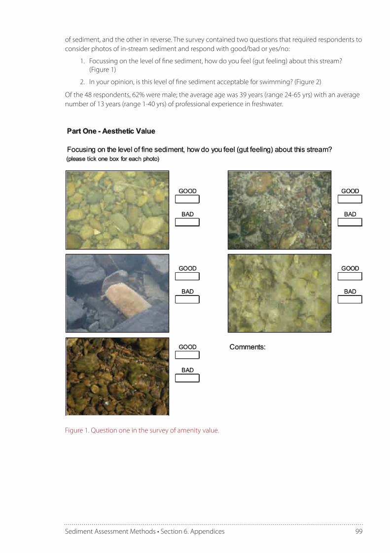
99Sediment Assessment Methods • Section 6. Appendices
of sediment, and the other in reverse. The survey contained two questions that required respondents to consider photos of in-stream sediment and respond with good/bad or yes/no:
1. Focussing on the level of fine sediment, how do you feel (gut feeling) about this stream? (Figure 1)
2. In your opinion, is this level of fine sediment acceptable for swimming? (Figure 2)
Of the 48 respondents, 62% were male; the average age was 39 years (range 24-65 yrs) with an average number of 13 years (range 1-40 yrs) of professional experience in freshwater.
Part One - Aesthetic Value
Focusing on the level of fine sediment, how do you feel (gut feeling) about this stream?(please tick one box for each photo)
GOOD GOOD
BAD BAD
GOOD GOOD
BAD BAD
GOOD Comments:
BAD
Part One - Aesthetic Value
Focusing on the level of fine sediment, how do you feel (gut feeling) about this stream?(please tick one box for each photo)
GOOD GOOD
BAD BAD
GOOD GOOD
BAD BAD
GOOD Comments:
BAD
Figure 1. Question one in the survey of amenity value.

100 Sediment Assessment Methods • Section 6. Appendices
Part Two - Swimming Value
In your opinion, is this level of suspended sediment acceptable for swimming?(please tick one box for each photo)
YES YES
NO NO
YES YES
NO NO
Comments:YES
NO
Part Two - Swimming Value
In your opinion, is this level of suspended sediment acceptable for swimming?(please tick one box for each photo)
YES YES
NO NO
YES YES
NO NO
Comments:YES
NO
Figure 2. Question two in the survey of amenity value.
6.3 Details of the boosted regression tree model used to predict variation in fine sediment cover6
Source data
Sediment data used in model development was sourced from the Freshwater Fisheries database (http://www.niwa.co.nz/our-services/databases/freshwater-fish-database). The sediment response variable was calculated from a bankside estimate of the relative proportion of substrate size classes. Environmental variables were sourced from the FENZ database and included segment and catchment
6 This research was conducted by Joanne Clapcott and Eric Goodwin (Cawthron Institute) as part of a Ministry of Science and Innovation funded project on Cumulative Effects (C01X1005)
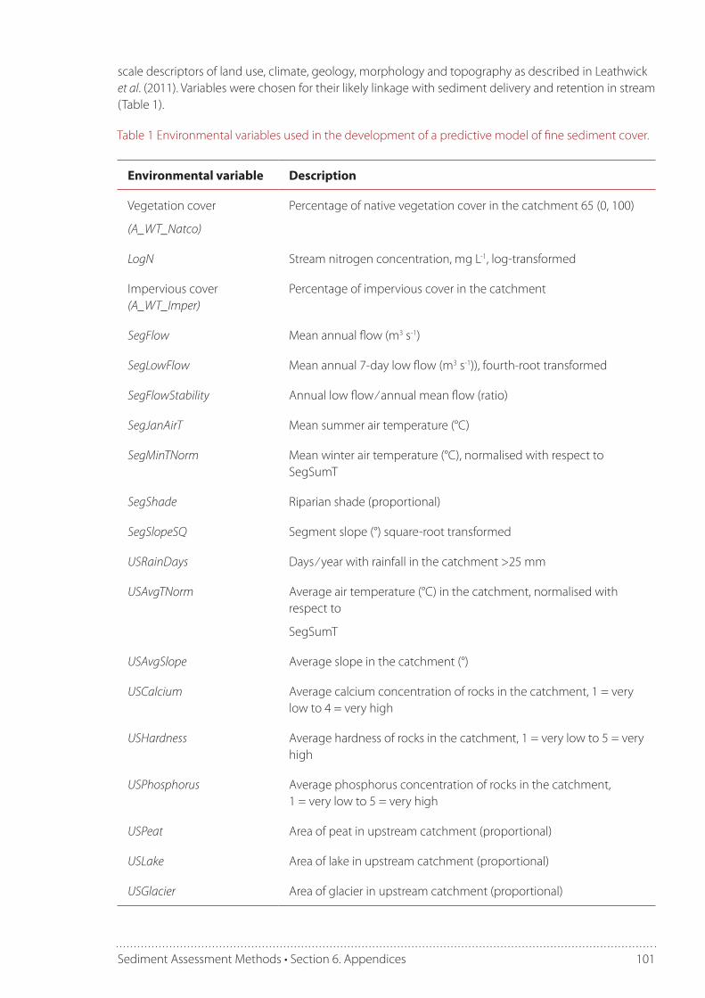
101Sediment Assessment Methods • Section 6. Appendices
scale descriptors of land use, climate, geology, morphology and topography as described in Leathwick et al. (2011). Variables were chosen for their likely linkage with sediment delivery and retention in stream (Table 1).
Table 1 Environmental variables used in the development of a predictive model of fine sediment cover.
Environmental variable Description
Vegetation cover
(A_WT_Natco)
Percentage of native vegetation cover in the catchment 65 (0, 100)
LogN Stream nitrogen concentration, mg L-1, log-transformed
Impervious cover (A_WT_Imper)
Percentage of impervious cover in the catchment
SegFlow Mean annual flow (m3 s-1)
SegLowFlow Mean annual 7-day low flow (m3 s-1)), fourth-root transformed
SegFlowStability Annual low flow ⁄ annual mean flow (ratio)
SegJanAirT Mean summer air temperature (°C)
SegMinTNorm Mean winter air temperature (°C), normalised with respect to SegSumT
SegShade Riparian shade (proportional)
SegSlopeSQ Segment slope (°) square-root transformed
USRainDays Days ⁄ year with rainfall in the catchment >25 mm
USAvgTNorm Average air temperature (°C) in the catchment, normalised with respect to
SegSumT
USAvgSlope Average slope in the catchment (°)
USCalcium Average calcium concentration of rocks in the catchment, 1 = very low to 4 = very high
USHardness Average hardness of rocks in the catchment, 1 = very low to 5 = very high
USPhosphorus Average phosphorus concentration of rocks in the catchment, 1 = very low to 5 = very high
USPeat Area of peat in upstream catchment (proportional)
USLake Area of lake in upstream catchment (proportional)
USGlacier Area of glacier in upstream catchment (proportional)

102 Sediment Assessment Methods • Section 6. Appendices
Data preparation
1. From the Freshwater Fisheries database Mud and Silt were summed in a new metric, FINES, ranging from 0-100%.
2. Data entries from lakes, ponds, lagoons, swamps, tarns, estuaries, reservoirs, dams, deltas, wetlands and oxbows were systematically deleted. The rationale for deleting non-flowing habitats was that the fine sediment distribution would be driven by a relationship between hydrodynamics and slope different to that in flowing waters. Many deleted entries had 100% FINES.
3. All data collected from and post 1990 was collated. The rationale was twofold; data prior to this time may not reflect the contemporary cover of in-stream sediment, and environmental data available for predictive modelling is compiled from 1996-2000 satellite data.
4. An investigation of the spatial distribution of resulting entries showed an obvious gap in representation of the Fiordland region. A further spatial analyses revealed only 64/100 FENZ classes were represented by post1990 data opposed to 68/100 FENZ classes in the complete dataset. Three of the four additional FENZ classes were present in pre1990 Fiordland data. It was determined unlikely that land-use had changed in that region pre and post 1990 and therefore all data entries from flowing waters with Easting less than 2080000 (i.e., Fiordland) were re-added to the dataset.
5. Finally, data entries with missing predictors (e.g., A_WT_NATCO = NA) were removed and the FINES variable was arc-sine transformed to improve normality. Final dataset N = 10026.
Modelling contemporary sediment cover
Several boosted regression tree models were explored including:
1. The use of all 19 predictor variables.
2. The substitution of geological variables (USPeat and USGlacier) with River Environment Classification (REC) variables Geology and Source of Flow.
3. A reduced set of the top 12 explanatory variables following a back step model selection procedure (simplify script).
There was no significant reduction in predictive power between a 19-predictor model and a 12-predictor model. Furthermore, the back step procedure suggested at least another three variables could be left out, but a preference was for increased explanatory power rather than the most parsimonious model (i.e., the 12-predictor model). None of the geological descriptors (FENZ or REC) were significant contributors to the models.
After deciding on model parameters, a boosted regression tree model was then fitted with a learning rate of 0.05 and a tree complexity of five and using Gaussian model error. The final model had a cross-validation error of 0.67 (se = 0.005) and explained 45% of the variance in % fine sediment cover (n = 10,026), which suggest good model performance. Fitted functions for the 12 most important explanatory variables are shown in Figure 1. These fitted functions were used to predict fine sediment cover in each NZREACH stream segment in New Zealand.

103Sediment Assessment Methods • Section 6. Appendices
0 10 20 30 40
-0.2
0.0
0.2
0.4
USAVGSLOPE (20%)
fitte
d fu
nctio
n
0.0 0.2 0.4 0.6 0.8 1.0
-0.2
0.0
0.2
0.4
A_WT_NATCO (12.7%)
fitte
d fu
nctio
n
8 10 12 14 16 18 20
-0.2
0.0
0.2
0.4
SEGJANAIRT (12.2%)
fitte
d fu
nctio
n
0 100 200 300 400 500 600
-0.2
0.0
0.2
0.4
SEGFLOW (9.9%)
fitte
d fu
nctio
n
-8 -6 -4 -2 0 2
-0.2
0.0
0.2
0.4
USAVGTNORM (7.4%)
fitte
d fu
nctio
n
-2 -1 0 1 2
-0.2
0.0
0.2
0.4
LOGNCONC (7%)
fitte
d fu
nctio
n
1 2 3 4 5
-0.2
0.0
0.2
0.4
SEGSLOPESQ (6.7%)
fitte
d fu
nctio
n
-4 -2 0 2 4
-0.2
0.0
0.2
0.4
SEGMINTNOR (5.6%)
fitte
d fu
nctio
n
0.0 0.1 0.2 0.3 0.4 0.5 0.6
-0.2
0.0
0.2
0.4
SEGFLOWSTA (5.3%)
fitte
d fu
nctio
n
0 20 40 60 80 100
-0.2
0.0
0.2
0.4
USDAYSRAIN (5.1%)
fitte
d fu
nctio
n
0 1 2 3 4 5
-0.2
0.0
0.2
0.4
USHARDNESS (4.4%)
fitte
d fu
nctio
n
0.0 0.2 0.4 0.6 0.8 1.0
-0.2
0.0
0.2
0.4
A_WT_IMPER (3.7%)
fitte
d fu
nctio
n
0 10 20 30 40
-0.2
0.0
0.2
0.4
USAVGSLOPE (20%)
fitte
d fu
nctio
n
0.0 0.2 0.4 0.6 0.8 1.0
-0.2
0.0
0.2
0.4
A_WT_NATCO (12.7%)
fitte
d fu
nctio
n
8 10 12 14 16 18 20
-0.2
0.0
0.2
0.4
SEGJANAIRT (12.2%)
fitte
d fu
nctio
n
0 100 200 300 400 500 600
-0.2
0.0
0.2
0.4
SEGFLOW (9.9%)
fitte
d fu
nctio
n
-8 -6 -4 -2 0 2
-0.2
0.0
0.2
0.4
USAVGTNORM (7.4%)
fitte
d fu
nctio
n
-2 -1 0 1 2
-0.2
0.0
0.2
0.4
LOGNCONC (7%)
fitte
d fu
nctio
n
1 2 3 4 5
-0.2
0.0
0.2
0.4
SEGSLOPESQ (6.7%)
fitte
d fu
nctio
n
-4 -2 0 2 4
-0.2
0.0
0.2
0.4
SEGMINTNOR (5.6%)
fitte
d fu
nctio
n
0.0 0.1 0.2 0.3 0.4 0.5 0.6
-0.2
0.0
0.2
0.4
SEGFLOWSTA (5.3%)
fitte
d fu
nctio
n
0 20 40 60 80 100
-0.2
0.0
0.2
0.4
USDAYSRAIN (5.1%)
fitte
d fu
nctio
n
0 1 2 3 4 5
-0.2
0.0
0.2
0.4
USHARDNESS (4.4%)
fitte
d fu
nctio
n
-0.2
0.0
0.2
0.4
LOGNCONC (7%)
fitte
d fu
nctio
n
1 2 3 4 5
-0.2
0.0
0.2
0.4
SEGSLOPESQ (6.7%)
fitte
d fu
nctio
n
-4 -2 0 2 4
-0.2
0.0
0.2
0.4
SEGMINTNOR (5.6%)
fitte
d fu
nctio
n
0.0 0.1 0.2 0.3 0.4 0.5 0.6
-0.2
0.0
0.2
0.4
SEGFLOWSTA (5.3%)
fitte
d fu
nctio
n
0 20 40 60 80 100
-0.2
0.0
0.2
0.4
USDAYSRAIN (5.1%)
fitte
d fu
nctio
n
0 1 2 3 4 5
-0.2
0.0
0.2
0.4
USHARDNESS (4.4%)
fitte
d fu
nctio
n
0.0 0.2 0.4 0.6 0.8 1.0
-0.2
0.0
0.2
0.4
A_WT_IMPER (3.7%)
fitte
d fu
nctio
n
Figure 1 Fitted functions for the 12 most explanatory variables explaining deviance in percent sediment cover at the reach scale.
Modelling ‘reference’ sediment cover
Land-use predictors were the 2nd, 6th and 12th most explanatory variables in the sediment cover model (Figure 1). The fitted functions for the relationship between sediment cover and land-use predictors were as expected, with increasing fine sediment in response to decreasing native vegetation cover and impervious cover, and increasing sediment in response to increasing land-use intensity, i.e., increasing predicted nitrogen levels (within 95% of the data distribution). As such a 3-predictor model was developed where the responses were directionally constrained and the output from this 3-predictor model was used as a fixed offset in a model to predict sediment cover in the absence of land use.
The 3-predictor model was fitted using a learning rate of 0.05 and a tree complexity of five. The fitted model used 750 trees and had a cross-validation error of 0.51 and explained 26% (se = 0.008) of the variance in % fine sediment cover. The constrained fitted functions are shown in Figure 2.
0.0 0.2 0.4 0.6 0.8 1.0
-0.3
-0.1
0.1
0.3
A_WT_NATCO (48.5%)
fitte
d fu
nctio
n
-2 -1 0 1 2
-0.3
-0.1
0.1
0.3
LOGNCONC (30.6%)
fitte
d fu
nctio
n
0.0 0.2 0.4 0.6 0.8 1.0
-0.3
-0.1
0.1
0.3
A_WT_IMPER (20.8%)
fitte
d fu
nctio
n
0.0 0.2 0.4 0.6 0.8 1.0
-0.3
-0.1
0.1
0.3
A_WT_NATCO (48.5%)
fitte
d fu
nctio
n
-2 -1 0 1 2
-0.3
-0.1
0.1
0.3
LOGNCONC (30.6%)
fitte
d fu
nctio
n
0.0 0.2 0.4 0.6 0.8 1.0
-0.3
-0.1
0.1
0.3
A_WT_IMPER (20.8%)
fitte
d fu
nctio
n
Figure 2. Fitted functions for percent sediment cover at the reach scale in response to three land-use variables (relative explanatory deviances are in parentheses).

104 Sediment Assessment Methods • Section 6. Appendices
The 3-predictor model output was used as a fixed offset in a new model with the remaining nine environmental variables used to explore variation in sediment cover in the absence of land use, i.e., in reference condition. This offset model was fitted using a learning rate of 0.05 and a tree complexity of five. The fitted model used 1550 trees and had a cross-validation error of 0.64 (se = 0.004) and explained 42% of the variance in % fine sediment cover. The low decrease in model performance compared to the former inclusive 12-predictor model provides confidence in fixed model output. Fitted functions from the offset model were used to predict fine sediment cover in each NZREACH stream segment in New Zealand based solely on environmental variability, i.e., expected ‘reference’ values in the absence of land use.
6.4 Volumetric Quorer methodThis method is termed Suspendible Benthic Sediment Volume (SBSV). This method is the same as the standard Quorer method (http://www.niwa.co.nz/our-science/freshwater/tools/estimating-deposited-fine-sediment) except that the level of fine suspendible sediment is measured by settling overnight in a conical glass rather than gravimetrically (as SIS = dry mass minus ash-free dry mass) per unit area of streambed. Adapted champagne flutes (as in this example) can be used if standardised Imhoff cones are unavailable.
Collected Quorer samples are transferred into Imhoff cones or champagne flutes (c. 170 ml volume) and left to settle overnight. Volumes of acrylic flutes can be marked by scoring the outside of each flute to graduate the levels at appropriate volumes (e.g., 1, 2.5, 5, 7.5, 10, 15, 20, 25, 30, 40, 60, 80, 100, 120, 140 ml) using a craft knife and label using a water-proof pen (Figure 1).
Figure 1. Graduated acrylic champagne flutes used to measure settled volume of Quorer method samples.
In initial trials using this method it was possible to distinguish between the volumes of coarse particles that settled in a layer below fine material (Figure 1) and between organic sediment that settled above the inorganic sediment. It will be useful to evaluate whether this is a practicable and meaningful measure in future trials.
Initial trials indicate that acrylic flutes are preferable to glass ones because they are physically robust and are easily etched allowing for individual calibration. Use of these relatively inexpensive settling vessels enables lots of replication and many samples to be processed simultaneously (Figure 2).

105Sediment Assessment Methods • Section 6. Appendices
Figure 2. Reading settled volumes on multiple samples from contrasting sites from Whatawhata Research Centre streams.
The settled volume of fine sediment after overnight settling and the total sample volume are recorded and both used to calculate SBSV:
Areal SBSV (litres/m2 of streambed)
= 1000 x (settled sediment volume (ml) / total sample volume (ml)) x average water depth in the Quorer sampler (m).
Volumetric SBSV (litres/m3 of streambed)
= Areal SBSV / (average stirred depth – average water depth).
Example calculations for SBSV:
Attribute Data or calculated value
Settled sediment volume (ml) 8
Total sample volume (ml) 140
Average water depth (m) 0.1
Average stirred depth (m) 0.15
Areal SBSV (litres /m2 streambed) 5.7
Volumetric SBSV (litres /m3 bed sediment) 114.3


Deposited fine sediment occurs naturally in the beds of rivers and streams, but human activities can accelerate sedimentation. Excess sediment directly affects the health of a waterway, decreasing its mauri or life-supporting properties. The protocols and guidelines presented in this document provide robust and nationally consistent tools to assess the effects of deposited sediment on the in-stream values of New Zealand's waterways.
ISBN: 978-0-473-20105-0 (Print) ISBN: 978-0-473-20106-7 (Online)