SeDFAM: Semiconductor Demand Forecast Accuracy Modelmetin/Research/forecast_s.pdf · SeDFAM:...

SeDFAM: Semiconductor Demand Forecast

Accuracy Model

Metin Cakanyıldırım

School of ManagementUniversity of Texas at Dallas

Robin Roundy

School of Operations ResearchCornell University

IIE Portland Conference 2003

UTDallas.edu/∼Metin 1

Semiconductor Industry

Industry Characteristics

• High Technology - Competition leads toShort Product Life Cycles and Frequent Line Width Changes

• Volatile Demand

• Fab financing: tool prices

Business Contribution: Quantify Risk and Uncertainty

• Capacity acquisition

– Customer service: meet market demand– Tool utilization


Goals of the Research

• Forecast Modeling

1. Covariances of product demands; substitutes - complements

2. Signal deteriorating forecasts

3. Forecast simulation


Demand Modeling

• A hierarchical model:Product families by general functionality, i.e. memoryProducts by functionality and line width, i.e. memory CMOS 12

• Level of detail driven by capacity planning

• For families with persistent demands

• Products have transient demands

• Family demands are often correlated: Memory and CPU chips

• Correlations can often be strong

1. Correlation among the products of the same familye.g. between (memory,CMOS8) and (memory,CMOS10)

2. Correlation among the products of different product familiese.g. between (memory,CMOS10), (X86,CMOS10)


Notation

• p, q: families (e.g. ASICS, X86)

• tec , tec+: a line width and its successor (e.g. CMOS10, CMOS12)

• (p, tec): a product (e.g. (memory, CMOS10))

• dp,tecs,t : demand forecast made in s for t for a product (p, tec)

• dps,t : demand forecast made in s for t for a family p

dps,t =

∑

tec

dp,tecs,t

• H : forecast horizon


Inputs to Forecast Evolution

Forecast history for a product (p, tec)

Lags Jan ..... Sep ..... Dec

0 dp,tecjan,jan ..... dp,tec

sep,sep ..... dp,tecdec,dec

.. .. ..... ..... ..... .....

t − s = 2 dp,tecnov,jan ..... d

p,tecjul,sep ..... d

p,tecoct,dec

.. .. ..... ..... ..... .....

H dp,tecjan−H,jan ..... d

p,tecsep−H,sep ..... d

p,tecdec−H,dec


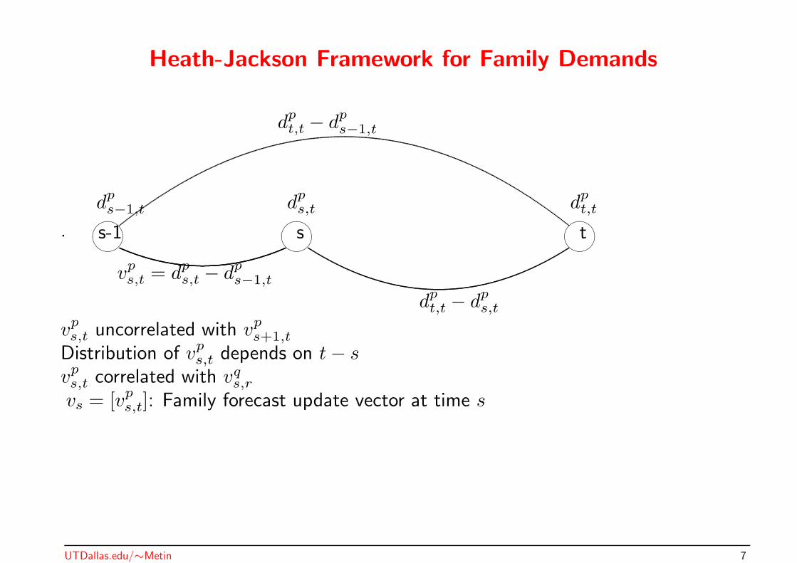
Heath-Jackson Framework for Family Demands

��s-1

dps−1,t

��

s

dps,t

��

t

dpt,t

dpt,t − d

ps−1,t

vps,t = d

ps,t − d

ps−1,t

dpt,t − d

ps,t

vps,t uncorrelated with v

ps+1,t

Distribution of vps,t depends on t − s

vps,t correlated with vq

s,r

.

vs = [vps,t]: Family forecast update vector at time s


SeDFAM

Fractional Forecasts: fp,tecs,t : Fraction of demand for family p line width tec

or shorter, forecasted from s for t

fp,tecs,t =

∑linewidth≤tec d

p,tecs,t

dps,t

Analyzing Fractional Forecasts

• Heath-Jackson approach is not directly applicable

• Apply a nonlinear transformation mapping Fractional Forecasts to Perceived Ages

• Apply Heath-Jackson to Perceived Age Forecasts


Computing Perceived Ages from Fractional Forecasts

6

0

R(δ)

1

-

δ

fp,tecs,t

δp,tecs,t L

Perceived age update up,tecs,t = δ

p,tecs,t − δ

p,tecs−1,t


Perceived Age Update Vectors

• Construct iid update vectors

u14s = [uX86,14

s,s , ..., uX86,14s,s+H−1, u

Mem,14s,s , ..., u

Mem,14s,s+H−1, u

PPC,14s,s , ...]

iid: updates for different technologies are independent

u16s = [uX86,16

s,s , ..., uX86,16s,s+H−1, u

Mem,16s,s , ..., u

Mem,16s,s+H−1, u

PPC,16s,s , ...]

iid: updates created in different time periods are independent

u16s+1 = [uX86,16

s+1,s+1, ..., uX86,16s+1,s+H, u

Mem,16s+1,s+1, ..., u

Mem,16s+1,s+H, u

PPC,16s+1,s+1, ...]

��:

v Data is missing if (X86, 16) production ends before s + H

• utecs ∼ N(0,Σ) , use EM (Expectation Maximization) algorithm by Schafer (1997)


Summary: SeDFAM Estimation Procedure

Inputs : Demand forecasts, dp,tecs,t

1. Estimate family forecast update covariance matrix, Λ

2. Fit ramp function R to fractional forecasts

3. Compute perceived age forecasts δp,tecs,t = R−1(fp,tec

s,t )

4. Estimate perceived age forecast update covariance matrix, Σ(using the EM algorithm)

5. Use R , Λ , Σ to compute variances and covariances of demandsas seen in period r


Step 5 of SeDFAM Estimation Procedure

• Computing variance of R(δp,tecs,t ) is complicated because R is not linear

• Options: Monte-Carlo Sampling or Numerical Integration

– R is a quadratic spline with 3 knots– Knots define regions of integration in <2

• We use Monte-Carlo Sampling


Flowchart for Simulating Forecasts

Test accuracy of SeDFAM in estimating capacity demand covariances

Perceived Ages

δp,tecr,t = ∆p,tec

r,t |=r.

?

Perceived Age Updates

U tecs = (Up,tec

s,t ) ∼ N(0, Σ).

?

Perceived Age Forecasts ∆p,tecs,t = ∆p,tec

s−1,t + Up,tecs,t .

?Fractional Demand Forecasts F

p,tecs,t = R(∆p,tec

s,t )

?

Family Demands

dpr,t = D

pr,t|=r.

?

Family Demand Updates

Vs = (V ps,t) ∼ N(0, Λ).

?

Family Demand Forecasts Dps,t = D

ps−1,t + V

ps,t.

?Product Demand Forecast D

p,tecs,t = D

ps,t(F

p,tecs,t − F

p,tec+s,t ), see (??).


Biases

• Lag bias: E(update) 6= 0, simple modification of forecast evolution

• Nonlinearity bias: Fractional forecasts = R (perceived ages)perceived ages unbiased implies fractional forecasts biasedSmall when R is close to linear.


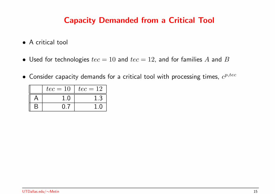
Capacity Demanded from a Critical Tool

• A critical tool

• Used for technologies tec = 10 and tec = 12, and for families A and B

• Consider capacity demands for a critical tool with processing times, cp,tec

tec = 10 tec = 12

A 1.0 1.3B 0.7 1.0


Experimental Design

Simulation Model��

Historical Forecasts up to period now

?

Estimated covariance matrixof forecasts generated in now

HHHHHHHHHHHHj

N independent evolutionsfrom period now on

?

True covariance matrixof forecasts generated in now


Heuristics

• Allocation: Family variances are allocated to technologies

– Proportional to forecasted volume

• Proportion: Update is proportional to the forecast

dp,tect−h,t − d

p,tect,t

dp,tect−h,t

∼ ξh

– Assume ξh , h = 1..H has the same distribution for ∀ (p, tec) ∀ t

– [Variance of error in dp,tect,t ] = (dp,tec

now,t)2var(ξt−now)

• Neither Allocation nor Proportion capture correlations (time-wise or amongfamilies)


Results: Capacity Acquisition

• Customer Service: P(meet customer demand) targeted at 84.1 %.

Method LT=2 LT=4 LT=6 LT=8 LT=10 LT=12 AverSeDFAM 83.2 82.6 83.0 83.0 83.5 83.9 0.97Allocation 76.6 78.1 78.5 79.1 79.7 80.0 5.52Proportion 86.2 85.4 88.2 87.2 86.8 88.2 3.29

• Tool Utilization : E(excess capacity / mean demand for capacity)

Method LT=2 LT=4 LT=6 LT=8 LT=10 LT=12 AverTrue 22.9 34.4 33.6 35.5 33.9 33.1 -SeDFAM 22.1 32.8 33.0 34.5 33.4 32.8 1.1Allocation 18.8 29.1 28.5 30.5 29.5 29.1 5.4Proportion 32.8 38.5 40.7 40.7 37.8 38.5 11.4


Robustness Analysis

• Cs,t: forecast (from s for t) of the critical tool capacity required

• Γ: covariance matrix of [Cnow+1,now+1, ..., Cnow+H+1,now+H+1]

• Performance measure: F (Γ) = (Estimated Γ)−(True Γ)(True Γ)

Properties varied without significant effect on performance:

• Skewness of ramp curves

• Forecast horizon, H

• Magnitude of covariances in perceived age updates

• Correlations across families & time in family demand & age updates


Robustness Analysis: Forecast History

55 60 65 70 750

0.05

0.1

0.15

0.2

0.25

0.3

0.35

0.4

F(Γ

)

Starting Months for Replications

90 month aver. 60 month aver.

45 month aver.

30 month aver.

x, o, +, * : individual runswith 90, 60, 45, 30 months of forecast history

SedFAM estimates Γ more accurately with longer forecast history


Tests with Industrial Data

Model assumptions pass statistical tests with the industrial data

Perceived age stationarity tested visually:

0 5 10 15 20 25−15

−10

−5

0

5

10

15

Ramp age

Per

ceiv

ed a

ge u

pdat

e


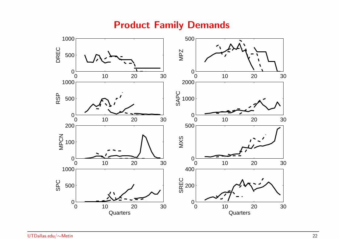
Product Family Demands

0 10 20 300

500

1000

DR

EC

0 10 20 300

500

MP

Z

0 10 20 300

500

1000

RS

P

0 10 20 300

1000

2000

SA

PC

0 10 20 300

100

200

MP

CN

0 10 20 300

500

MX

S

0 10 20 300

500

1000

Quarters

SP

C

0 10 20 300

200

400

Quarters

SR

EC


Data Analysis

• Select Families: SAPC, SREC, DREC, MXS

– Life Cycles for MPZ, RSP ended– Life Cycles for MPCN, SPC started

• Make demand stationary

Family SAPC SREC DREC MXSExponent 0.076 0.043 -0.0016 0.1192


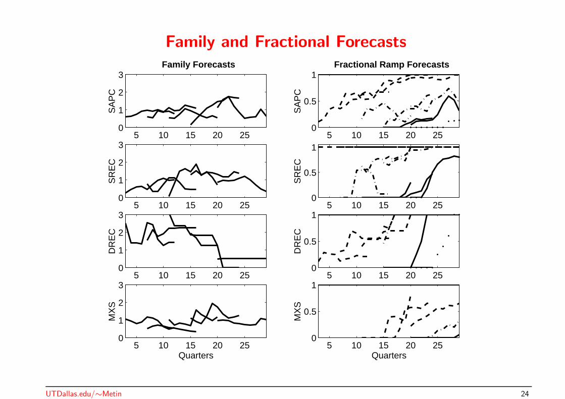
Family and Fractional Forecasts

5 10 15 20 250

1

2

3

SA

PC

Family Forecasts

5 10 15 20 250

0.5

1

SA

PC

Fractional Ramp Forecasts

5 10 15 20 250

1

2

3

SR

EC

5 10 15 20 250

0.5

1

SR

EC

5 10 15 20 250

1

2

3

DR

EC

5 10 15 20 250

0.5

1

DR

EC

5 10 15 20 250

1

2

3

Quarters

MX

S

5 10 15 20 250

0.5

1

Quarters

MX

S


Resolution of Uncertainty in Family Forecasts

1 1.5 2 2.5 30

0.2

0.4

0.6

0.8

1 Family Demand Coefficient of Variation in Years

DR

EC

, mea

n=28

9

1 1.5 2 2.5 30

0.2

0.4

0.6

0.8

1

SA

PC

, mea

n=34

71 1.5 2 2.5 3

0

0.2

0.4

0.6

0.8

1

Forecast Lag in Years

MX

S, m

ean=

133

1 1.5 2 2.5 30

0.2

0.4

0.6

0.8

1

Forecast Lag in YearsS

RE

C, m

ean=

143


Resolution of Uncertainty in Perceived Age Forecasts

1 1.2 1.4 1.6 1.8 2 2.2 2.4 2.6 2.8 30

1

2

3 Perceived Age Forecasts, Standard Deviation of Error in Years

DR

EC

1 1.2 1.4 1.6 1.8 2 2.2 2.4 2.6 2.8 30

1

2

SA

PC

1 1.2 1.4 1.6 1.8 2 2.2 2.4 2.6 2.8 30

1

2

Forecast Lag in Years

SR

EC


Correlations in Family Demands

DREC SAPC MXS SREC1 2 1 2 1 2 1 2

DREC-1 100 -91 73 74 70DREC-2 100 -61 -75 -66 -67

SAPC-1 -91 100 -85 -70 -81 -81SAPC-2 100

MXS-1 73 -61 -85 100 96 99 100

MXS-2 -75 -70 96 100 95 97

SREC-1 74 -66 -81 99 95 100 100

SREC-2 70 -67 -81 100 97 100 100

DREC and SAPC subtitutes. MXS and SREC complements.


Correlations in Perceived Ages

DREC SAPC SREC1 2 1 2 1 2

DREC-1 100 61 -72DREC-2 61 100 -83

SAPC-1 -72 100 55SAPC-2 55 100 -54 -57

SREC-1 -83 -54 100SREC-2 -57 100


Effectiveness of SeDFAM in estimating Γ, in %

• All key assumptions are statistically verified

• Correlations: Strong or weak

• Update Frequency

– Only impacts SeDFAM performance thru amount of data available– Bayesian approach; Computationally stable, but sensitive to prior

Sample size Size of F (Γ) by Quarters Aver

Λ, Σ Λ, Σ 30 32 34 36 38 40 F (Γ)

Annu,Quar,Bay. 5 , 10 10x10 63 51 35 37 40 42 44.7

Semi,Quar,Bay. 10 , 22 14x14 44 39 28 27 29 38 34.2

Quar,Quar,Bay. 20 , 50 16x16 44 32 32 29 30 27 32.3

Quar,Quar,Fre. 20 , 50 16x16 21 18 15 14 11 13 15.3


Conclusion

SeDFAM

• accurately estimates forecast error variances & correlations

• is robust

• requires about 48 periods of history for good performance

• benefits

1. quantify risk and uncertainty2. signals deteriorating forecasts3. forecast simulation


SeDFAM: Semiconductor Demand Forecast Accuracy Modelmetin/Research/forecast_s.pdf · SeDFAM:...

Documents

Transcript of SeDFAM: Semiconductor Demand Forecast Accuracy Modelmetin/Research/forecast_s.pdf · SeDFAM:...