SECURITY CLASSIFICATION OF THIS PAG = REPORT …AFATL/DLCM 9. PROCUREMENT INSTRUMENT IDENTIFICATION...

UNCLASSIFIED

SECURITY CLASSIFICATION OF THIS PAG =

REPORT DOCUMENTATION PAGE 1 la. REPORT SECURITY CLASSIFICATION

UNCLASSIFIED 2a. SECURITY CLASSIFICATION AUTHORITY

,2b. DECLASSIFICATIOIM/DOWNGRADING SCHEDULE

4. PERFORMING ORGANIZATION REPORT NUMSER(S)

„^R85-926546-20

lb. RESTRICTIVE MARKINGS

3 DISTRIBUTION/AVAILABILITY OF REPORT

Approved for Public Release; Distribution Unlimited

5. MONITORING ORGANIZATION REPORT NUMBER(S)

AFATL-TR-85-37

6a. NAME OF PERFORMING ORGANIZATION

United Technologies Research Cen

6b. OFFICE SYMBOL (If applicable)

:er

7a. NAME OF MONITORING ORGANIZATION

Air Force Armament Laboratory

6c. ADDRESS {City, State, and ZIP Code)

Silver Lane East Hartford, Connecticut 06108

7b. ADDRESS (Oty, State, and ZIP Code)

Eglin Air Force Base Florida, 32542-

8a, NAME OF FUNDING/SPONSORING ORGANIZATION

Aeromechanics Division

8b, OFFICE SYMBOL (If applicable)

AFATL/DLCM

9. PROCUREMENT INSTRUMENT IDENTIFICATION NUMBER

F08635-83-C-0287

8c. ADDRESS (Ory, State, and/JP Code;

AFATL/DLCM Eglin AFB, FL

10, SOURCE OF FUNDING NUMBERS

PROGRAM ELEMENT NO,

-61101F

PROJECT NO,

ILIR

TASK NO,

83

WORK UNIT ACCESSION NO

04 11 TITLE (Include Security Classification)

Composite Integral Response Sensing

12 PERSONAL AUTH0R;S)

J. R. Dunphy, G. Meltz and R. M. Elkow 3a, TYPE OF REPORT

Final Report 13b, TIME COVERED

FROM_Aug 82_ TO Mar 85

14 DATE OF REPORT {Year, Month, Day) September 1985

15, PAGE COUNT

114 16, SUPPLEMENTARY NOTATION

Availability of this report is specified on verso of front cover.

17, COSATI CODES

FIELD

11 13

GROUP

04 13

SUB-GROUP

18, SUBJECT TERMS {Continue on reverse if necessary and identify by block number)

Fiber Optic Strain Gage,

Flight Control Systems Distributed Strain Sensing

19. ABSTRACT (Continue on reverse if necessary and identify by block number)

This document describes the investigation of a new concept for measurement of distributed strain. Implementation of the technique utilizes a fiber optic device with twin, coupled cores, a single input and a single output. Multiple wavelength operation of the sensor yields a diagnosis of the waveguide coupling perturbations imposed by mechanical disturbances. A general theory for the device has been derived in the form of an integral equation that relates the sensor core contrast to an arbitrary bending strain or curvature. In many cases of interest the curvature is small and slowly varying. For these conditions theory shows that the core crosstalk spectrum is directly related to the Fourier

20. DISTRIBUTION/AVAILABILITY OF ABSTRACT

[a UNCLASSIFIED/UNLIMITED ED SAME AS RPT. D DTIC USERS

21. ABSTRACT SECURITY CLASSIFICATION

UNCLASSIFIED 22a. NAME OF RESPONSIBLE INDIVIDUAL

J. R. Cloutier 22b. TELEPHONE (Jnc/ude Area Code)

(904) 882-2961 22c. OFFICE SYMBOL

AFATL/DLCM

DDFORM 1473,84 MAR 83 APR edition may be used until exhausted.

All other editions are obsolete. SECURITY CLASSIFICATION OF THIS PAGE

UNCLASSIFIED

UNCLASSIFIED SECURITY CLASSIFICATION OF THIS PAGE

19. ABSTRACT (Concluded]

transform of the strain distribution on a cantilevered beam. This result pertains to a wing with gradual bends (radius of curvature large compared to arc length) while stipulating very practical requirements on potential sensor parameters (radius of curvature large compared to device beatlength). Two computer models were developed from the theory. One model provides a rudimentary simulation of a wing with arbitrary loading (cantilevered beam). It was used to prove that the Fourier transformation of the simulated sensor output matched the bending moment distribution. The second model was developed to calculate the sensor response for comparison with the demonstration experiments. Fiber optic devices were designed and fabricated for laboratory-scale tests. Sensor performance was diagnosed by techniques established in direct support of these demonstrations. Verification experiments performed with simple bending perturbations in the laboratory apparatus confirmed the general form of the sensor spectra predicted by the model.

UNCLASSIFIED SECURITY CLASSIFICATION OF THIS PAGE

LIBRARY RESEARCH REPORTS DIVISION NAVAL POSTGRADUATE SCHOOL MONTEREY, CALIFORNIA 93940

AFATL-TRril5=^:ZL»

Composite Integral Response Sensins:

J R Dunphy G Meitz R M Elkow

_UNrrEDjiCHNOLOG!ES RESEARCH CENTER *^!LVER LANE

EAST HARTFORD, CONNECTICUT 06108

SEPTEMBER 1385

FINAL REPORT FOR PERiOO AUGUST 1982 - MARCH 1985

3f^--

Approved for public release; distribution.unlimited

/>Air Force Armameiit Laboratory^ /AIR FORCE SYSTEMS COMMAND * UNITED STATES AIR FORCE •EGLIN AIR FORCE BASE. aORIDA

'i

/■!.:,-<,; lUA'i _\ .i:::~-M'

NOTICE

When the Government drawings, specifications, or other data are used for any purpose other than in connection with a definitely related Government procurement operation, the United States Government thereby incurs no respon- sibility nor any obligation whatsoever; and the fact that the Government may have formulated, furnished, or in any way supplied the said drawings, specifications, or other data, is not to be regarded by implication or otherwise as in any manner licensing the holder or any other person or corporation, or conveying any rights or permission to manufacture, use, or sell any patented invention that may in any way be related thereto.

This report has been reviewed by the Public Affairs Office (PA) and is releasable to the National Technical Information Service (NTIS). At NTIS, it will be available to the general public, including foreign nations.

This technical report has been reviewed and is approved for publication.

FOR THE COMMANDER

^<^^S^o^ 'DONALD C. DANIEL Chief, Aeromechanics Division

Even though this report may contain special release rights held by the controlling office, please do not request copies from the Air Force Armament Laboratory. If you qualify as a recipient, release approval will be obtained from the originating activity by DTIC. Address your request for additional copies to:

Defense Technical Information Center Cameron Station Alexandria, Virginia 22314

If your address has changed, if you wish to be removed from our mailing list, or if the addressee is no longer employed by your organization, please notify AFATL/ DLCM Eglin AFB FL 32542.

Copies of this report should not be returned unless return is required by security considerations, contractual obligations, or notice on a specific document.

/"

PREFACE

This program was conducted by the United Technologies Research Center,

Silver Lane, East Hartford Connecticut, 06108 under Contract FO8635-83-C-0287

with the Air Force Armament Laboratory, Eglin Air Force Base, Florida 32542.

James R. Cloutier (DLCM) managed the program for the Armament Laboratory. The

program was conducted-during the period from August 1982 to March 1985.

The Public Affairs Office has reviewed this report, and it is releasable to

the National Technical Information Service (NTIS), where it will be available to the general public, including foreign nationals.

i

(Reverse is Blank.)

TABLE OF CONTENTS

Section Title Page

I INTRODUCTION 1

II THEORETICAL DEVELOPMENT 5 1. Introduction 5 2. General Model oiE a Twin-Core Distributed Strain Sensor . . 12 3. Crosstalk Spectra of Pure Bends 18

III EXPERIMENTAL DEVELOPMENT 47 1. Approach 47 2. Apparatus 47 3. Phase-II Data and Comparison With Theoretical Model .... 51

IV SUMMARY AND RECOMMENDATIONS 59

APPENDICES

A PHASE-I DATA 61

B IMPROVEMENTS 73

REFERENCES 105

111

LIST OF FIGURES

Figure Title Page

1 Wing Load Monitor 2

2 Wing Load Compensation 3

3 Cross Section of a Twin-Core Fiber-Optic Distributed Strain Sensor 6

4 Crosstalk in a Twin-Core Fiber 7

5 Lowest-Order Modes in a Twin-Core Fiber 8

6 Curved Section of a Bent Twin-Core Fiber 10

7 Geometry of Twin-Core Sensor Bent by Two Circular Disks 20

8 Crosstalk Spectral Analysis 23

9 Spectrum of a Single Bend With a Large Radius of Curvature 24

10 Spectrum of a Single Bend 25

11 Spectrum of a Single Bend 26

12 Spectrum of a Single Bend. Both Cores Illuminated Equally 27

13 Spectrum of a Single Bend. One Core Illuminated 28

14 Spectrum of a Single Bend. One Core Illuminated (f=l) 29

15 Spectrum of Single Bend. Core Contrast Transformed Into a Function of Wavelength 30

16 Spectrum of a Single Bend. Core Contrast Quadratic Dispersion Causes Ripple in the Principal Spectrum Feature. Fiber Lengths Increased by a Factor of 5 Over Figure 4 . ., 33

iv

LIST OF FIGURES (CONTINUED)

Figure Title Page

17 Distributed Strain Sensor Attached to Cantilever Beam 34

18 Cantilever Beam Geometry 35'

19 Moment Diagram and Strain Distribution 36

20 Shear Diagram 37

21 Variation in Mode Coupling Parameter 38

22 Crosstalk Spectrum of a Uniformly Loaded Cantilever Beam 39

23 Sine Transform of Q(K) , . 40

24 Strain Distribution in a Cantilever Beam With Point and Distributed Loads 41

25 Shear Diagram of Cantilever Beam in Fig. 24 ... , 42

26' Crosstalk Spectrum of Cantilever Beam with Point and Distributed Loads 43

27 Sine Transform of Q(K) 44

28 Measurement Concept 48

29 Demonstration Experiment: Data Acquisition System 49

30 Demonstration Perturbations 50

31 Phase-II: Short Right Angle Bend, Sample A04.5SQC/ 11.27.29 52

32 Phase-II: Long Right Angle Bend. Sample A04.5SQC/ 7.25.8.2 54

33 Phase-II: Single Loop. Sample A04.5SQC/12.18 , . 55

34 Phase-II: Single Loop. Sample A04.5SQC/12 .18 . . 56


Figure Title Page

35 Phase—II: Right Angle Bend; Round Core. Sample AORDC/12.5.6 58

A-1 Response of Straight Fiber. L=100 cm; Sample A045QC/DSS3.141 62

A-2 Crosstalk Spectrum vs. Sensor Mounting. Sample AO4SQC/0552.151/DSS1.152 63

A-3 Length Scaling in Crosstalk Spectrum. Sample A04SQC/ DSS4.31/DSS4.51/D8S4.61 64

A-4 Crosstalk Spectra: Right-angle Bend (straight reference case). Sample A04SQC/DSS2.101 67

A-5 Crosstalk Spectra: Right-angle Bend (perturbed case). Sample A04SQ/DSS2.81 68

A-6 Serpentine Demonstration 69

A-7 Crosswalk Spectra: Serpentine Bend. Samples A04SQC/ DSS3.141/DSS3.15/DSS3.201 70

A-8 Crosstalk vs. Loop Radius. Fixed Wavelength = 6328A. Sample A04SQC/DSS7.00 71

B-1 Twin-Core Geometry 74

B-2 Beat Length of Original Square Core 75

B-3 Crosstalk vs. Dimensional Control 76

B-4 Crosstalk Improvement Comparison 78

B-5 Crosstalk Near Asymmetric Mode Cut Off 80

B-6 Asymmetric Mode Filter. L = 30.8 inches; O.D. = 61 ym. Sample A02.4SQC/8.29 81

VI


Figure Title Page

B-7 Asymmetric Mode Filter 82

B-8 Parameter Assessment: Straight fiber. Sample A045SQ/DSS7,191 ' 83

B-9 Signal Processing: Rectangular Window Response . . 85

B-10 Signal Processing: Concept of Padding Crosstalk Array 86

B-11 Signal Processing: Concept of Windowed Crosstalk Array 87

B-12 Signal Processing: Candidate Window Functions . . 89

B-13 Signal Processing: Kaiser-Bessel Window Response 90

B-14 Signal Processing: Dolph-Chebyshev Window Response 91

B-15 Signal Processing: 3-Term Blackman-Harris Window Response 92

B-16 Signal Processing: 4-Term Blackman-Harris Window Response 93

B-17 Signal Processing Application 95

B-18 Right-Angle Bend Data (Fig. A-5). Processed ... 96

B-19 Serpentine Bend Data (A=2 in.; Fig. A-7). Processed 97

B-20 Serpentine Bend Data (A=7 in.; Fig. A-7). Processed 98

B-21 Sensor Calibration: Force Response. Sample A04.55Q, X=633 nm, O.D. = 0.0045 inch, Lg^=34.204, Lrp = 46.3 cm 100

Vll

LIST OF FIGURES (CONCLUDED)

Figure Title "^ Page

B-22 Sensor Calibration: Length Change Response: Sample A04.55Q, X=600.8 nm, O.D.=0.0045 inch . . 101

B-23 Xg vs X Dispersion: Straight Sensor. Sample A04.55Q, L=35.5 inches 103

LIST OF TABLES

Table Title Page

B-1 Relative Window Performance 94

B-2 Experimental Dispersion Equation 104

VI11

EXECUTIVE SUMMARY

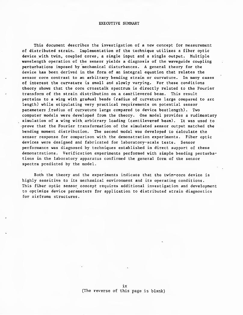
This document describes the investigation of a new concept for measurement

of distributed strain. Implementation of the technique utilizes a fiber optic

device with twin, coupled cores, a single input and a single output. Multiple wavelength operation of the sensor yields a diagnosis of the waveguide coupling

perturbations imposed by mechanical disturbances. A general theory for the

device has been derived in the form of an integral equation that relates the

sensor core contrast to an arbitrary bending strain or curvature. In many cases

of interest the curvature is small and slowly varying. For these conditions

theory shows that the core crosstalk spectrum is directly related to the Fourier

transform of the strain distribution on a cantilevered beam. This result

pertains to a wing with gradual bends (radius of curvature large compared to arc

length) while stipulating very practical requirements on potential sensor

parameters .(radius of curvature large compared to device beatlength). Two

computer models were developed from the theory. One model provides a rudimentary

simulation of a wing with arbitrary loading (cantilevered beam). It was used to

•prove that the Fourier transformation of the simulated sensor output matched the

bending moment distribution. The second model was developed to calculate the

sensor response for comparison with the demonstration experiments. Fiber optic

devices were designed and fabricated for laboratory-scale tests. Sensor

performance was diagnosed by techniques established in direct support of these

demonstrations. Verification experiments performed with simple bending perturba-

tions in the laboratory apparatus confirmed the general form of the sensor

spectra predicted by the model.

Both the theory and the experiments indicate that the twin-core device is

highly sensitive to its mechanical environment and its operating conditions.

This fiber optic sensor concept requires additional investigation and development

to optimize device parameters for application to distributed strain diagnostics

for airframe structures.

IX

(The reverse of this page is blank)

SECTION I

INTRODUCTION

This report describes a new type of fiber optic sensor for the measurement

of distributed loads on composite components. Since the sensor ideally measures the bending moment distribution of the structure to which.it is attached or embedded, a detailed decomposition of the load distribution could be potentially

derived to yield the location and magnitude of isolated mechanical disturbances positioned at arbitrary points along its length.

The device consists of a single fiber optic filament containing two closely-

spaced, crosstalking waveguides. An optical source with multiple wavelengths

illuminates the single sensor input and a processing unit analyzes the signal

from a detector unit that corresponds to the light emitted from the end of the

sensor. This report identifies the processed sensor output as the Fourier

Transform of the shear distribution imposed by the structural loading. When the

sensor output is interpreted with knowledge of the structure's elastic proper-

ties, important parameters such as distributed strain or deflection become available.

The material and geometry of this new sensor are compatible with critical

applications within composites. It can be as small as 0.002 inches in diameter

and meters long, making it suitable for embedding in graphite/epoxy composite

skins for large structures. Its small transverse dimension assures negligible

void generation within the matrix material, while the high temperature consti-

tuents eliminate sensitivity to curing procedures. Finally, its dielectric

characteristics promise to immunize the diagnostic function against electro- magnetically induced noise.

Potential advantages to be derived from application of this new sensor are

significant. For instance, such a sensor might be embedded within the wing of an

aircraft with varying numbers and weights of stores (Figure 1). During opera-

tion, the flight dynamics of the aircraft may be altered by the load distribution

on the wings. An automatic compensation scheme could be configured to place the

aircraft's control surfaces in feedback loops that use the fiber sensor measure-

ments, as well as other critical flight data, to derive correction factors for

their adjustments. Realization of such an approach (Figure 2) would relieve the

pilot of the need to correct for variable flight characteristics as stores are

released or changed. Long term records of the fiber sensor measurements would

also provide basic data on long term fatigue parameters relevant to the wings'

structural strength. Finally, we anticipate a major advantage to result from the

instrumented wings' ability to self-diagnose its response to new types of stores,

providing allowable specification ranges for the modified requirements.

to

Fiber optic sensors

Photo detectors

Composite covering

Composite covering

Store 1 Store 2

Non-composite core Laser diode

illuminators

Sensor data

Ptioto detectors Laser diode

illuminators

Sensor data

store 2

Non-composite core

■o

'c TO

Store 1 load store 2

A load JlJL Signal

conditioning "

Position

Signal L conditioning

<D X) 3 store 2

■ ■■■

C load O) A

Position

Figure 1. Wing Load Monitor

Sensor data case 1

Sensor data case 2 Signal

processor

Flight control

computer

Servo- actuator

compensation

Actuator 1

Actuator 2 Flight

control surfaces

Figure 2. Wing Load Compensation

This report summarizes our investigations to model and to demonstrate the

basic response of this promising device. The modelling proceeds from basic

sensor/bend interaction to complex predictions for the entire output spectrum of

the device attached to a cantilevered beam representation of a wing. On the

other hand, the experimental work focuses on evaluation of sensor characteristics

in simple and complex configurations implemented on small-scale laboratory bench

apparatus. The goal of the measurements was to provide verification of the

fundamental theoretical model. In our experiments the general form of the

predicted spectra was confirmed. One important physical effect, polarization

sensitivity, has not been included in the formulation and is suspected as the

cause of complications during the benchmark experiments. Each issue and

accomplishment is reviewed in the following text.

SECTION II

THEORETICAL DEVELOPMENT

1. INTRODUCTION

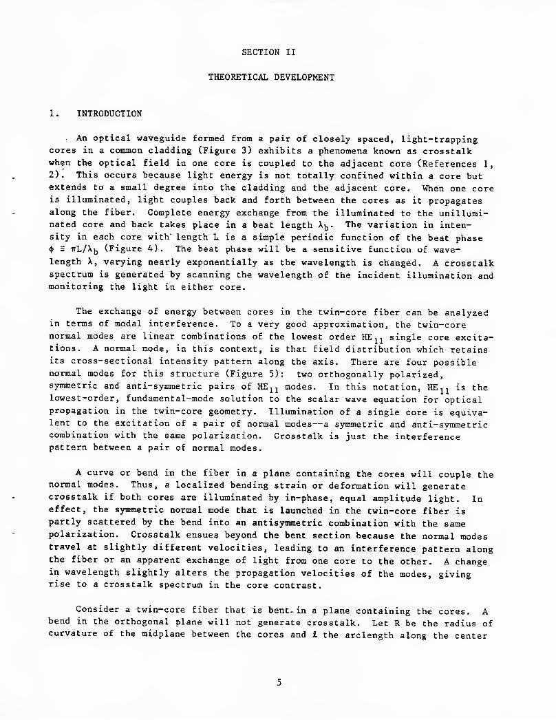
An optical waveguide formed from a pair of closely spaced, light-trapping

cores in a common cladding (Figure 3) exhibits a phenomena known as crosstalk

when the optical field in one core is coupled to the adjacent core (References 1,

2). This occurs because light energy is not totally confined within a core but

extends to a small degree into the cladding and the adjacent core. When one core

is illuminated, light couples back and forth between the cores as it propagates

along the fiber. Complete energy exchange from the illuminated to the unillumi- nated core and back takes place in a beat length X^. The variation in inten-

sity in each core with length L is a simple periodic function of the beat phase <j) = irL/Xjj (Figure 4). The beat phase will be a sensitive function of wave-

length X, varying nearly exponentially as the wavelength is changed, A crosstalk

spectrum is generated by scanning the wavelength of the incident illumination and monitoring the light in either core.

The exchange of energy between cores in the twin-core fiber can be analyzed

in terms of modal interference. To a very good approximation, the twin-core

normal modes are linear combinations of the lowest order HE,, single core excita-

tions. A normal mode, in this context, is that field distribution which retains

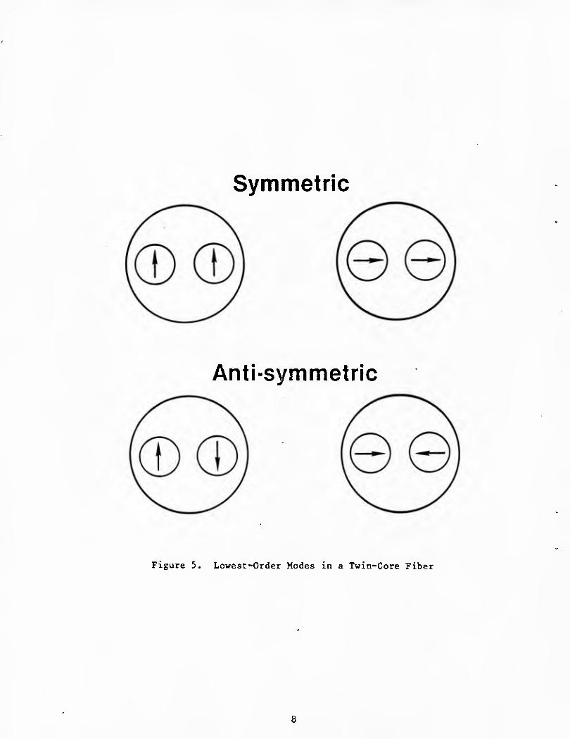
its cross-sectional intensity pattern along the axis. There are four possible

normal modes for this structure (Figure 5): two orthogonally polarized,

symmetric and anti-symmetric pairs of HE^^ modes. In this notation, HE,, is the

lowest-order, fundamental-mode solution to the scalar wave equation for optical

propagation in the twin-core geometry. Illumination of a single core is equiva-

lent to the excitation of a pair of normal modes—a symmetric and anti-symmetric

combination with the same polarization. Crosstalk is just the interference pattern between a pair of normal modes.

A curve or bend in the fiber in a plane containing the cores will couple the normal modes. Thus, a localized bending strain or deformation will generate

crosstalk if both cores are illuminated by in-phase, equal amplitude light. In

effect, the symmetric normal mode that is launched in the twin-core fiber is

partly scattered by the bend into an antisymmetric combination with the same

polarization. Crosstalk ensues beyond the bent section because the normal modes

travel at slightly different velocities, leading to an interference pattern along

the fiber or an apparent exchange of light from one core to the other. A change

in wavelength slightly alters the propagation velocities of the modes, giving rise to a crosstalk spectrum in the core contrast.

Consider a twin-core fiber that is bent, in a plane containing the cores. A

bend in the orthogonal plane will not generate crosstalk. Let R be the radius of

curvature of the midplane between the cores and £ the arclength along the center

Figure 3. Cross Section of a Twin-Core Fiber-Optic Distributed Strain Sensor

Light intensity ^

Light "ZZZZZl vzzzzz

Twin core fiber

1.0 1.5 Distance L/Xu

Figure 4. Crosstalk in a Twin-Core Fiber

Symmetric

Anti-symmetric

Figure 5. Lowest-Order Modes in a Twin-Core Fiber

line (see Figure 6). The fields in the fiber can be approximated (References 1,

3, 4) by a linear combination of the isolated, unperturbed HEj^^ modes in a

straight fiber:

E = ai{l)Ei + a2(Ji)E2 (1)

The amplitudes, a^ and ^2, obey the following pair of coupled mode equations:

da 1 _ —^ = -j(l-d/2R)(Ti/X^)a2 - iB^a-df2R)a^ (2)

-^ = -j(l+d/2R)(Tr/X^)a^ - j6^(l+d/2R)a2 (3) dA

If we assume d/2R « 1, as is always the case, then the coupling coefficients

(1 - d/2R)''T/Xjj become equal and power is conserved in the forward traveling

modes. In the case of pure bending, that is if R is constant, the solution to

Equations (8) and (9) can be expressed in the following matrix form (Reference

4):

(4)

where

X = cos(K£) + j(6/K) sin(Kii) (5)

Y = (TT/X^)/K sin(KJl) (6)

with

and

K = J(Tr/Xj^)2 + 62 (7)

2T 6 = — ni(d/2R) . (8)

The transfer matrix for a series of pure bends and straight sections is obtained

directly from Equation (4) by matrix multiplication.

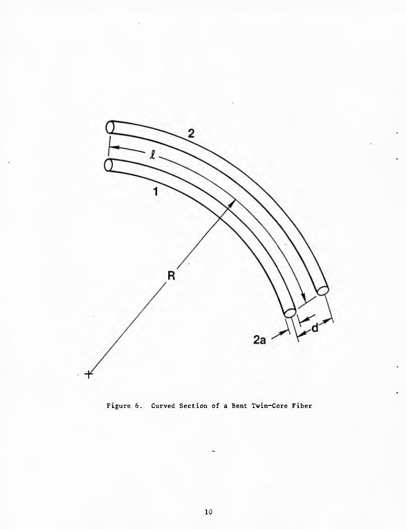
Figure 6. Curved Section of a Bent Twin-Core Fiber

10

In many cases of interest 6 << n/X^ and the transfer matrix T of a uniform bend reduces to

T =

cos (K£)

-j sin(K£)

-j sin(KJl)

cos(K£)

+ jC^b/Rg) sin(KJl)

1 0

0 -1

(9)

where Rg is an effective radius of curvature given by Rg = R(X/n^d). From

Equation (9), we can analyze the effect of a bend on a normal mode. It can be seen that

:)v^"^'"'(! + jC^fc/Rg^ sin(K£) 0 (10)

that is, a bend of effective radius Rg delays the symmetric mode by the arc

length of the bend and generates a phase quadrature asymmetric normal mode having

a strength proportional to the ratio of the beat length and the effective

curvature 1/Rg- The two modes give rise to small oscillating components in

each core as X^ and therefore K is swept by varying the wavelength. In a like

manner, an asymmetric mode is advanced in phase by the bend and generates a phase quadrature symmetric mode. If the arc is followed by a straight section of fiber

of length £Q, each mode acquires an additional phase advance or delay, as can

be seen from Equation (9) in the limit 1/Rg -»• 0. The net result is a core

contrast Q(K) formed by the ratio of the difference in light intensities in the

cores to the total power transmitted by the fiber that is proportional to the

curvature of the arc and consists of two harmonic components related to the

distance of the arc from the end of the fiber and its total length:

Q(K)

* ai ai - LLIL 3,0 3.0

oiH-i • S.nH<^ = - (6/K) {COS[2K(£Q+£)] - cosilKl^)} (11)

Thus, the mode coupling due to the bend produces harmonic components in the

spectrum of Q. If the wavelength is scanned over a narrow band then TT/X^, is

approximately a linear function of X and the spectral lines at (£Q+£) and i^ have the characteristic sine function shapes, of the Fourier transform of a pulse- modulated wave.

11

The effective radius Rg can be directly related to the bending strain or

moment in a beam. If the fiber sensor is a distance C above the neutral axis of

the beam then

1/(R-C) = M/EI (12)

where M is the bending moment, E is Young's Modulus and I is the moment of

inertia. The bending strain

e = C/(R-C) - C/R (13)

To summarize, a bend in the sensor caused by a localized strain disturbance

generates a harmonic component in the core contrast with a frequency determined

by the length and location of the bend from the detector and with a spectral

amplitude proportional to the bending strain.

The preceeding analysis can be generalized to the case of nonuniform bends

by approximating the deflection curve by a spline function; that is by a piece-

wise continuous set of cubic functions. The principle results will be stated in the next section which also gives some specific examples of the crosstalk

spectrum for various disturbances.

2. GENERAL MODEL OF A TWIN-CORE DISTRIBUTED STRAIN SENSOR

The relationship between the core contrast spectrum and the bending strain

or the curvature of the fiber is in the form of an integral equation in the most general case. It is derived from the matrizant solution of a linear system of

first order differential equations (Reference 5). The two coupled mode Equations

(2) and (3) for the amplitudes of the fields in the cores are an example of such

a system. If the mode conversion due to the varying curvature is weak, that is,

if ^b/^e ^^ ■'• throughout the length of the sensor, then the integral equation, which is generally in the form of a convergent series of product integrals

(Reference 6), reduces to a simple Fourier integral that can be solved by well

known transform methods. An alternate approach to solving the integral equation

is to model the bending curve by spline functions; that is by a set of piecewise

smooth cubics whose coefficients are determined by the crosstalk spectrum. This

is possible because the coupled mode equations have an analytical solution if the

curvature is a linear function of the fiber length (Reference 7). There are some

other isolated cases where the connection between the bending strain and the

spectrum can also be obtained in closed form; however, the curvature must match

one of the known solutions of the Ricatti equation (Reference 8).

12

The first step in developing a general model for the effect of variable

fiber curvature on the core contrast spectrum is to introduce a local normal mode

transformation. At every point along the fiber we can reexpress the ^n mode individual core amplitudes a^ and a2 in terms of new variables Aj^ and A2 that are

the amplitudes of the local two-core fiber modes. This is accomplished by means

of an orthogonal transformation

Tîi) = ■cos(?/s) sin(5/2)'

-sin(C/2) cos(5/2)

(14)

ipplied to the vector (AJ^CI), A2(1))'' of individual core amplitudes, where

cos2(5/2) = - [I+S/K], 2

(15)

sin2(5/2) = - [1-5/K], 2

(16)

and

5/K = /v^ (\/^)' (17)

A new set of coupled-mode equations for Aj^ and A2 follows from Equations (2) and

(3) by using

= X - • (18)

where

n-l _ cos(5/2) -sin(C/2)

sin(5/2) cos(5/s)

(19)

The take the form

Â^(Jl)N

A2(Jt)j

-j(6^+K) 1/2 V o

-111 5 -j(VK)

Ikîl)^

S^2^^\

(20)

13

where the mode coupling parameter ?', which is derived by differentiating Equations (15) and (16), is

g' = —= 2(6/K)'/[l-(«/K)]2 (21)

Along a straight section of fiber or an arc of constant curvature C' = 0 and no mode conversion takes place. In this case the solution of Equation (20) is

A2(il)/ \ A2(0)e o

Note, however, that along an arc the normal modes differ from those of a straight

section. If (^b/^e) ^ 0» then

^A^(£)\ _. /(ai(0)+a2(0)Je ^

l//2"e'^^°| ) (23)

k^H)/ \(a2(0)-a^(0)Je ^

and to lowest order in (^^/Rg)

[ai(0)+a2(0)]e ^+ -^ (X^/Re^t^l^0)-^2^0)]^ (20

[a2(0)-a^(0)]e^"'''"^ -i (X^/R^) [a^ (0)+a2(0) je''"'

Thus, the normal modes in a section of constant curvature, an arc, are linear combinations of the symmetric and asymmetric modes of a straight section - a result obtained in a somewhat different way in the preceeding section (see Equations (9) and (10).

The local normal mode equations can be simplified further by applying phase

transformations to each of the mode amplitudes. Let

14

j / (6 ±K)dz

^1,2<^^) = A^^2(^^*^ ° (25)

and

u = 2 / K d2 (26)

This reduces Equation (20) to

1 d5

2 du

1 dS

2 du

iu gj

-ju

'B^(U)

B2(u)

(27)

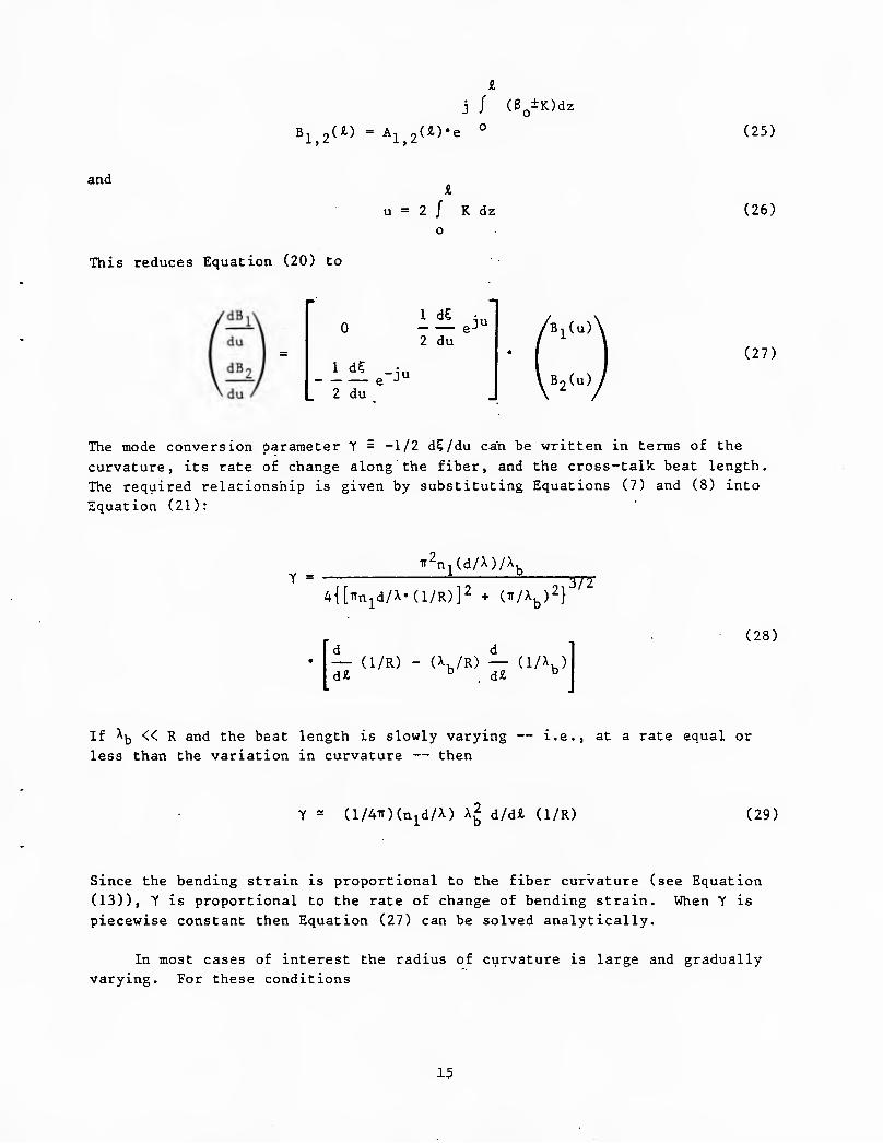
The mode conversion parameter T = -1/2 d5/du can be written in terms of the

curvature, its rate of change along the fiber, and the cross-talk beat length.

The required relationship is given by substituting Equations (7) and (8) into

Equation (21):

Y = T^n^(d/X)/X^

4{[Trn^d/X-(l/R)]2 + (ii/X^)' 37T

— (1/R) - (X,/R) — (1/X ) di ° di °

(28)

If X^ « R and the beat length is slowly varying

less than the variation in curvature — then

— i.e., at a rate equal or

y = (l/4Tr)(n^d/X) X2 d/d£ (1/R) (29)

Since the bending strain is proportional to the fiber curvature (see Equation

(13)), Y is proportional to the rate of change of bending strain. When Y is

piecewise constant then Equation (27) can be solved analytically.

In most cases of interest the radius of curvature is large and gradually

varying. For these conditions

15

= 2K£ (30)

where < - ^/^h is the cross-talk spatial frequency, and

y = (TT/4)(d/X)(l/<^) — (1/K) d£

(31)

Applying these approximations to Equation (27), we can simplify the reduced

normal equations to the following form:

— = P(£)B (32)

; P(Jl) =

0 -e'(£)/K-e

-j2<il e'(£)/K'e

j2Kil

0

where ^"i^) = 2<T(2.) is apart from a constant factor the rate-of-change of the

bending strain along the fiber.

The solution to Equation (32) is given in terms of the matrizant ^Q(P)

Bii) = ti^ • B(0) (33)

where I A Z2

"^(P) = I + / P(zpdz^ + / P(z2) / P(z;L^dz-^dz2 + (34)

is an absolutely and uniformly convergent infinite series of matrices with the identity matrix I as the leading term. Each term is derived from a successive approximation to the solution of Equation (33). The solution can be thought of as composed of a series of successively higher-order multiple mode conversions. Convergence takes place quickly if Y^^^ « 1; then

fi^(P) = I +

r j2<z -, -/ e'(z)/<'e dz^

f -j2<z / e'(z)/<'e dz

L O

(35)

16

The amplitudes of the individual core modes at the end of a fiber of length L can

be written in terms of the truncated matrizant Equation (35) and the incident

illumination expressed as a linear combination of local normal modes by using Equations (25) and (18):

(L)N

a2(L)

= l//2 -j(B +K)L

1 -e" J2<L

j2<L

• fJ* • B(0) (36)

To illustrate the form of the integral equation relating E(£) to the cross talk

spectrum, consider the case of equal and in-phase illumination of both cores. In

this example only the symmetric mode is launched and Equation (36) reduces to

(L)N a -/ e'(z)/ <e J2K:(L-Z)

dz

I -j(6 +K)L/ = 1//2 e °

a2(L)/ 1 +/ e'(z)/<e

o

j2<(L-z) dz.

(37)

The core contrast is given by

Q(<) = (a2^2 ~ Si-^a-^)/(a-^a^ + a2a2)

L

= 2 / e'(z)/<«cos[2<(L-z)]dz

o

(38)

The final result is obtained by integrating Equation (38) by parts:

Q(K) = (2/K) [e(L) - e(0) cos 2<L]

L

- 4 / e(z)sin[2K(L-z)]dz

o

(39)

17

If the strain (curvature) is zero at the ends of the sensor, then Equation (39) shows that the cross talk spectrum — i.e., the core contrast considered a function of the wavelength through the spatial frequency < — is directly related to a folded Fourier sine transform of the unknown strain distribution e(z). Thus, we have solved the general form of the integral Equation (36) by reducing it to a Fourier transform pair.

When a small fraction f of the antisymmetric mode is also launched

B(0) = (l,f)'' and Equation (36) becomes

r r^ i2Kz j2KL / r^ ^ -j2Kz 1-f / e'/Ke dz-e (f+ J e'/<e d

= l//2 -j(e +IC)L/

r^ i2<Z J2KL / ,^ ^ ^1-f / e'/<e dz+e (f+ / e'/<

o \ o

-J2KZ e dz

(40)

The corresponding expression for core contrast is

2 { 1 r^ . j2ic(L-z) Q(<) = T- * Re < (1-f^) J e (z)/Ke dz

+ f e -e (41)

Equation (41) can be solved iteratively if f « 1 by using the solution to Equation (39) as a first approximation. When f is not small, i.e., of order one, then Equation (41) must be solved numerically. It is a nonlinear equation relating the real and imaginary parts of the Fourier transform of the bending strain ^{H) to Q(<). In order to solve it the Hilbert transform relationship must be used to eliminate the real or imaginary part of the transform from the equation. In most instances this is not necessary since the incident illumination can be selected to have nearly equal amplitudes in each core, insuring

f « 1.

3. CROSS-TALK SPECTRA OF PURE BENDS

Any disturbance composed of pure bends or arcs of constant curvature joined by straight sections of fiber can be analyzed by multiplying the crosstalk transfer matrices of each section, forming the core contrast function from the output core amplitudes and Fourier transforming the result to obtain the crosstalk spectrum. In this section we develop and carryout these computations for several specific examples selected to model the experimental geometries and predict the measured crosstalk spectra.

18

a. Model of Right Angle Bend

Consider a twin-core fiber of total length L bent by a circular disk of

radius r located between straight sections of fiber of lengths î, and ^2 (see Figure 7). The incident illumination can be decomposed into a sum of normal

modes

a^(0)>

a2(0) :)•■(.: (42)

A straight section of fiber delays and advances the normal modes by the cross-

talk beat phase î = '^/^b'^l °^ ^^^ length i-i- The curved section is

illuminated by

aâ^y

,^2^^1^

= e -j*l

+ fe J^

A circular arc has a transfer matrix of the form

(43)

T =

cos <}>.

-j(</K)sin +2

-j(K:/K)sin <t>2

cos lj>-

where

+ j(5/K)sin <^,

^2 = K-rs

1 0

0 -1

, K = = V^ 2+5 2

(44)

6 = (Tr/X)(n,d/r) , < = TT/X

At the end of the curved section

19

T

fi

Figure 7. Geometry of Twin-Core Sensor Bent by Two Circular Disks

20

fay

[cos<t'2 - j(</K)sin<t)2]e ^ + jfe ^(5/K)siti<|)2

1

+ |f[cos<|)2 + j(»c/K)sin<t'2]e'' ^ + 36"" ^(5/K)sin(t>2>' I ) (A5) ^- C) The remaining straight section introduces an additional phase change ^-^ = ir/X^'ilg (similar to the first section of fiber) but no further mode conversion.

Thus at the end of the fiber

il(L)>

= {[cos4>2-J(</K)sin*2]^ ^j^^ (6/K)sin*2} * a2a)/ \ -^ \1

+ ^f[cos<t>2+j(</K)sin<t>2]e ^ ^ +je ^ "^ (6/K)sin<|i25 * ( ) (^6)

A general expression for Q(<) can be derived from Equation (46) in a

straightforward way but it is lengthy and complicated when no assumptions are

made about the relative size of the geometrical and fiber parameters and the

nature of the incident illumination. It is more useful to exhibit a few limiting

cases that are tractable and which give rise to easily understood, recognizable

spectral features. More general results are easily obtained by direct matrix

multiplication of the appropriate chain of transfer functions and numerical

computation of the spectrum using an FFT algorithm.

If the radius of curvature is large, then <S/K << 1 and K = <. In this

limit, to lowest order in ^5/r

Q(K) = f cos(2<L) + l/2(6/K)(l-f2) (47)

•{cos[2<(s+Jl,)] - cos(,l<l^)]

21

Generally, there will be three spectral components in the transform of the core

contrast function located at distance from the origin proportional to the total

fiber length L, to the length £„ °^ the second straight segment and at a distance

directly related to the sum of the arc s and I2' The type of incident illumination, characterized by the fraction of the antisymmetric mode launched at the

input face of the fiber, influences the heights of the spectral lines but not

their location. If the fractional bandwidth of the wavelength scan AX/X is

narrow then the fractional variation in <, (AK/K), will also be small and the coefficient (<S/K) will be slowly varying compared to the cosine factors. It

follows that the line shapes will be sine functions having half-power widths and side lobe structures set by AK.

Before presenting some specific results to illustrate the variation in the

spectral features with fiber bending strain distribution, a brief review of the

discrete Fourier transform (DFT) scaling relationships and the Nyquist sampling

requirement in the present context is needed. Referring to Figure 8, the cross-

talk spectrum Q(£) is computed from the core contrast Q(K), for the moment

considered a function of < = ir/X^j, by sampling in intervals 6K between the

initial and final values of the beat wavenumber, ic^ and Kf, respectively. The Fourier variable conjugate to K is a length £. The scale of the spectrum as computed by the usual FFT algorithm is (£/ir). For example, if the most rapidly

varying component in the core contrast, is sin(K2£ ) then a peak will appear at

a frequency f^^^^^ = ^max''''' Thus by rescaling the frequency axis by ir, the spectrum becomes a direct function of the fiber length. The sampling interval in

< or equivalently in X must be small enough to insure that the longest length in

the spectrum is less than Tr/(26ic) . As shown in Figure 8 if the sampling

frequency f„ is written m/ir then m > 2£„^^ to insure the spectrum will not be

aliased. The resolution or the minimum detectable length feature is determined

by the bandwidth of the < scan (or equivalently AX = Xf - X^).

Experimentally, Q is a function of X and not <. The two variables are

related though through a crosstalk coupling factor which can be computed or

measured. If AX/Xf << 1, K is nearly a linear increasing function of X. A

linear transformation X(K) will leave the shape of the spectrum unaltered. Only

the "frequency axis" is rescaled by the slope of the X(<) relationship. If the

fiber is long enough, nonlinear terms in the power series expansion (or spline

fit) of X(K) will cause "chirping" and distort the shape of the spectral lines.

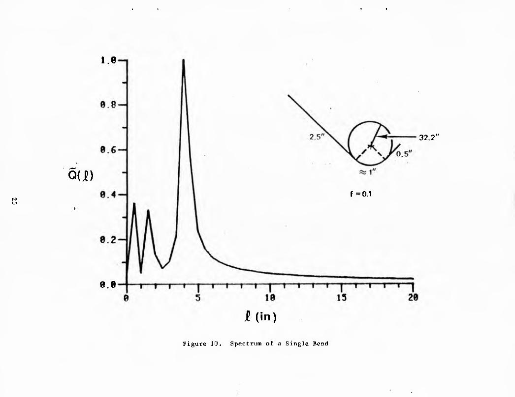
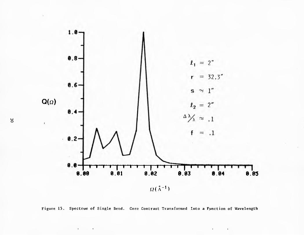
The various forms of the crosstalk spectral features generated by a single

bend (Figure 7) are shown in Figures 9 through 15. In each case the total fiber

length is held the same. The location of the bend, or the radius of curvature or

the illumination is varied. In the first three figures of the series. Figures 9

through 11, the illumination is held constant and the position and curvature of

the bend are changed. Three spectral features are expected since 6/K < 1 and

f = 0.1. As predicted by Equation (47) they are located at 4", approximately the

22

I t f »

Q(K) core

contrast

Beat K = Trl\ length

OK jY ma

' K X. X

Nyquist requirement

f«7r = i

f^ = m/7r

Min. resolution ^ 6f

= 1/A/<

Example:

Q(#c) = sin(K2i^3^)

^max = 27rf^ax = 2X^,^^

•'• ^max~'^max''^

^s>2imax^^

Figure 8. Crosstalk Spectral Analysis

i.e-n

tv3

32.2"

e.8-

0.6-

oa) 0.4-

0.2-

0.0

jP(m)

Figure 9. Spectrum of a Single Bend With a Large Radius of Curvature

* « * '•

t f • •

i.e

0(i)

32.2'

f =0.1

9.0

Kin)

Figure 10. Spectrum of a Single Bend

i.e-n

16.15"

Q(i)

i(in)

Figure 11. Spectrum of a Single Bend

¥ ♦ t *'

« « ■ *

i.e-i

Q(JC)

Figure 12. Spectrum of a Single Bend, Both Cores Illuminated Equally

• 20-1

• .15-

0.1t-

00

e.w-

Figure 13. Spectrum of a Single Bend. One Core Illuminated

i t « ♦

t * t I

• .2«-i

• .15-

QW •.!.-

•.w-

(i.pw

i Figure 14. Spectrum of a Single Bend. One Core Illuminated (f=l)

o

Q(")

I I i I I I—I I I I I t 1 I "] I

e.ee e.ei 8.02 e.83 0.89

i)(A-M

Figure 15. Spectrum of Single Bend. Core Contrast Transformed Into a Function of Wavelength

total length of the fiber, at the distance of the arc from the end of the fiber,

1 inch, and at 2 inches, the sum of the arc length and the second straight

section. The location of the spectral lines are determined by the location of

the bend along the fiber. The strain or radius of curvature is given by the

height of the two small peaks. The resolution in this example is somewhat coarse

since 1/AK = 0.25 mm implying 5f = 0.5 in. As a result, the heights of the peaks

are underestimated because of the large sampling interval. In Figure 10, the

position of- the arc is moved closer to the end of the fiber, all other parameters

are held constant. The pair of smaller amplitude lines shift to the appropriate

location as predicted by Equation (47). In the third figure in this group the

radius of curvature is halved. The pair of lines remain at the same point but

their amplitude is approximately doubled.

When the illumination of the cores is equal (f = 0) then only two peaks

appear in the spectrum. Figure 12 is a graph of the spectrum for the same

geometry in Figure 11 but f = 0. Again the two lines should have the same

amplitude but the resolution is not fine enough to sample at or very close to the

maxima. If the excitation is balanced, crosstalk occurs only when the fiber is bent.

When only one core is illuminated (f = 1) the effect of the bend on the

spectrum is second order in S/K. In this case

Q(<) = [l-l/2(6/ic)2] cos(2<L) + l/2(6/<)2{cos[2tc( £^-£2)

+ COS[2K(L-S)] - 1/2[COS[2K(£J^-£2+S)]

+ cos[2<(£^-£2-s)]}

and the spectrum has three minor lines grouped about £ = £-i-£2, plus a small component at £ = L-s.

Figure 13 is an example of a typical single bend spectrum when only one core

of the fiber is illuminated. Note the triplet of lines clustered about the point

^^-■^2 ~ ^ inches and the minor peak at L-s = 6 inches. Another example is shown in Figure 14. Here £^ is lengthened to 5 inches and £. is shortened by 1 inch to

keep the total length constant; the triplet is displaced by 2 inches from its position in Figure 13 and the other two lines remain in the same place, all in accord with Equation (48).

The spectral features become more complicated if the contrast is considered

to be a function of wavelength. Consider a typical term of the form cos (2<L).

If the fractional spectral width of the wavelength scan is small, Y can be

expanded is a power series in A:

31

0 ^ cr OJ (B cn

(B

0)

cr <B

13 r|

a cn r|

tB

O

c cr tB

cr r-' IU rt

O

c O a O

n o

o cr IB

CX

o rt

3-

O to

rt

a" (X

tB g" ^ o cw v£> (U C < rt O OQ N r-* r| a >-' IB r| c (X 3 (U o I-' c IB t-" o < Hi to

ft rt c w a CO P> (B i 13 3 fB W < D- [U C IX < r| fB rt rt o t-' cr c tB IB

:y rr rt 3* rt 3 (B 0 H- rt (U I-"- a a fB t-'- r-* r^ fB a r-i cn ^^ OQ r-" rt r-"

a> (t) m §■

, O r-' C ^

tB H rt O tB rt a t-"' cr > IB > cr o IX IB a IB tB > 3* O IB H-

cx O s a rt C rti D. C OQ u a ^ O rt O • r-' m o O >-• 13 3 3 i-t N> z 3 3 a- (B H- a. t1 X) m rt ttl rh n CO € rt X3 O --^ rt cn n fB

fO *-•■ ^ (B o (B rt O tB >■ rt (B cn X) rt IU K rt r-* H- < IB 3 >- 3" IB

w 3 X rt H' rt O 3- 3 r O rt t^ (B H- W rt CU IU o rt rt tB IB SL CX v.-^ fB H- cn

o 03 (B 3 o (B (U o I r| o D- rt a [U a r| 3- 3" i-l X !^ to 3 r-" a* 0) Klj a

•T3 ^ ?^ rt r-- rti po rt IU 13 C 1 cn 3 « XI O tB ^ 3" Hi J2 r-" CU

>—* H* 5^ rt nd (B rti 3 3" 3- H- rt tB a o rt cn H- IB to IU H- cn H- a c IB 13

(T) {jq t—* 3" H- (B H' O rt rt r*' tB tB a t-'- X> w o r| l-h 3 CX CO r-" >-• cr 3" OQ IU CU IU rh IB

d* c ro (B lu OQ cn O rt O 3-3 t-t [U c cr r| C O OQ rt H- XI O H- IU c •-< CX O

3"

O

t-t rt c ►n o a tB (X to (U rt [U r-* IB O 3 n IU 3 CU 3 rt 13 r| rt ti H-

•Tj (D o o rt o O 3 N3 (X >-'■ r| fB r-' IB rt cn IU r-" fB rt OQ tB IB cr IU cn

o CA o hh rt (B c (» rt o T; n tB m IU fB t—' ttl C X) a !^ rt rt IB rt O IU

c rt 3" rt r-- rt rti -< o rt rt X) IX ^ € t-*' r| t-i IU rt CO i-i- CO a" O rt H- rti rt

hO r| (U (B hJ H- O (U tB tB t1 XI CO fB IU cr IU fB r| p- Cfl a* o H- )-'• Hi 3" to n CX a" t-** Oi (D U) (B C cn o »« rh rt H- r| 3- rt IU < fB r-- t—' • r-i X) IU c 3 cn IB H- rt H- fB A

fD CO cy rt • rt r-" rt o rti a cr O O fB a (D rt IU fB IB XI I-" o rt OQ < 3* cn ^-^ h-t m X) (B rt HI c t-*- H- c X n CL r-- a rt <: n tB CU tB H 3* I-' 3 to IB o cn >-•

3 o {U CO rt y^ 13 £: o a rt H- 3 rt IB H- tB (-■• S tB rt r| H- fB IB H- H C IU ^—•

cn (X p ^ a M H' (B Tl r-- 3* H- tB H- a O I-'- a to a O r| rt IX H- XI 3 rh K- r-" CO M H> a. cn rt 3 a- H- H- H* fB o CU H- 1 3 OQ cr 3 H- W I-" 0) rt 13 13 OQ t--' IU I-"- cn fB II J3 fO r** t-h s OQ 3 O a rt a rt 0 rt fB IB cn cn cr CO 13 r-' rt rt o rt 3 H-

0) (J\ 3 O CU cr C OQ 3- rt 3- tB o XI a- a r| 3* IB O rt fB t-"- IB H- 3* CU H- IB o CU 7S

OQ rr ■a rt •-< r| CO fB o CL •n 1 3* cr v_^ t--- IB S t-h ^^ O cn 3 a O cn 3 CO o rt 3" "O rt (B X) H- Hi ►-'• [U CO fB XI X a H- rt c: O a* rt a •-< cn rt 0) 3 (l> CO H- < cr OQ X) cn O IX (U (U O cr rt rt 3 t-i" CU • CX O rt + (11 3- cr cn O 3 M M 3 iU cn ^ C IU IB a CX a cr S <: t--- c CU 3" rt 13 cn H- e rh 3*

p n) o n X CO Q to (U •v t^ 3' t^ I-*' ■ H IB a. IB X) r'- to rt r-" fB H- CU 3 tB fB en cn (JQ SU rt P> H- rti (B ^^ a r-" rt H- tB b tB H o cx rt 1—' rt rt t--- r-- r-" cr '^ rt r-*

i~h *-** i-i 3" r-* s O r| tB O 3" IU W CO IB rt K IB 3" rt o t-h -a fB H- A rt a" cn o o (B B) 3 H- 3' rt rt fB rt r| to O O (-■• 3* IB H- 3 fB H rt to IB OQ x-v O IB 13 '^ ^ »i p o- T3 rt n (B tB rt 1^- fB r-* rti O ^-s 3 IB fB XJ IU cr • CU o 3* XI 3 C >-• IB >' 3 [A H* o H* (B ID r| rt fB r| O l-ti rt 00 t-l •n 3 r| c rt CX IB tB rt ^^ rt r-i O

0) r*' CO CO o r-- (B (X tB a O a- IB H- O O O C rt C c O H- fB 3" t-"' rt >" 1 cn o OQ

rt

rt) r-- Pl D. M O |U IB OQ H cr rt < a IB r| o r-i rt 3 CO a IB 3 H O

(jj 3* t-h r) cn rt ^ O a H- c t--- n Hi 3 rt n C CO 3" H- I-"- CX IB rt IB H o IU IB C >-' N> o (U p' 3- o o a- a n a fB CL tB o t-l M fB fB CX Hi 3 CU t1 r-* VJ ja m a o

1—t § P3 H» (B ^-^ H- 3 tB cn n n a IB rt n IB 0 Z IU O OQ r-i IB Ul C rt ^—^ Di 3 l-t» !^ 3 CO rt Ti (X rt O 1—> rt rt rt < rti to r| o a i-h rt IU a* IU o r-t (U O. rt I-'- v-x rt h"- a- H- a* H- a ^O O t1 r-' IU tB H" a a CX 3" r-i CO CU fB CX § ttl +

H* OQ 3 (B g <* (D a> tB OQ 3 tB a CO n IU •~j o (X cr IU r-^ c rt H- IB 3 t^

P (B O' CL Ci. 13 OQ (B C O rt cn cn ^^ a- fB 3 ^ 3 rt 3" H- 3 CX CX cn a

IU 01 n H' o <: rt r( CO rt 3 a rt » • rt • tB O rt H- 3* fB CO IB rt cn to

cn rt- 3*

cn rt 3

CO

(B 3 fU rt

(B CX

a* tB

fB o 3* fB

a rt S H-

(X r| O O.

IX Hi

O

IB

O ttl H-

a* r--

C^ r-- t-i- o OQ

rh r| 1 1

OP r-( (D H a. a a. H- (U N3 t—* tB fB

^ cn W rt tn fB r-" cn 3 n 3" C 3 r-- 3 fB '' ^

c Q) H' o 3 rt r| 1—' cr cn O O cn rti C rt a" IU r| CU H- *• rt IU ^ >-' l-( H* o CJ" rt CO K OQ O ^ O fB fB ^ tB rt rt rt r-" CO rt H- r| rt •n r-i IB t-i a a> 3 o P (B rt (B IX o O (U OQ IU IB 3- X) ta tB rt t--- w t-i CU a" t--- t-h r-i h"- 3 fB 1

rt rt < rt Ck. rt cr H- a. c a a rt a n rt 1—' o rt cr IB 13 •o IB OQ IU C Hi cn 3 >• 03 (B (B (B fi> 3* (B (U z IB X) fB tB o o o H- TT rt IU c a rt t-l C O CO 13 o >-' r-( O. rt H- cr (B OQ o r-* a 1 3 rt o cn H- rt rt ex o fB I-l rr rt rt H- IB ^ o

• CT) n O 3

CO

(B

a. O ^

t1 (B

HI

a rt

to

w

c

r"*

a OQ

rH rt

rt

to O tB

a rt

(X

IB

rl

fB cn

a 0) rt

o r|

O

3 O

3

IB a.

CD o IB

r|

t~^* 3 o

IB O rt

rt

CU rt

3* fB

3 n rt o ,

1

O

r-»

O O. rt tti

Ml

1 Hi cn r-i PI rt 3' N)

o rt 0) H- 3" (X c rt M /-N o I-'- IB n r-i rti rt r| CJ1 O fB t-h ua i H-

i-t r| a. -^"-v CO (B C 3 o 3" rt X( CU -^ a" CX IU IU n c O 0 t--' H- IB • rh t-"- c t1

1-^ (U cn cn rt n n r| tB r*' (U a H*' w i--- rt r| n I-l Hi IU n O IU rt cr CU ^--y X)

(D cn (D rt tti (B rt o rl D- OQ a tn fB cr o <J CX H- CO cn Ul 3^ tB rt • fB

n rt H- fB H- H- D- H- P) cn a (U C OQ rt rt fB a IB rt IB fB s • H- r| H- CX

rt (0 CJ- 3 O . a a rt r( tB rt 3" IU IU to 3* H- a r-i CX cn O

I—* rh m C H- 3 a ,^>. CU /"^ tB 3" tB e- IB CO a rt ^->i fO CO rt fB IB H- 3 > X)

>-c; p cn ^ rt rt O ><a r-* OJ rt (B o cr cn IU o a O Z IB cn c 3 3* c H- fB r1 o r-' to tB ro l-tl c IB 6 IU 3 rt IU OJ O OQ n a o Hi ^^ ti t—'

!-•• n o (U O a rti • ^-^ r( r| o rt a a 3 rt X) to rt H- rt ttl t-" ■P- t--- cn D. rt rt 3 cn lu a. tB rt H- ex m IX ■ rt 13 H 3" rt 3 tB IB O ^ 13 fB

(D H* 3 H- O r-" rr H' p> -< r-* 3- o a. 3" r| C rt 3" O O 3 ^^ 13

3 O O (-•• CU 3" rti M ^^^ W H- tB a O H- tB O CX a" CU fB n rt rt OQ • I-' ^^ i-r 3 H* 3 P) a S (B t-h fB ^=> rt tn l-ti rt I-' X H- IU cn 3* • fB cn f-j' 3 O tB s_X H- (U O I-' tB H- 3 rt CO cr 13 IB IB tB

i-h (U rt H- (X cr r| • ' a rn c r-* a IB O tB tB 3 PI fB ^^ H* rt 3' 3 (B fB tB fij CL r"* cr a [U IU 3 1 3 CU rn O < -P- to m tB (U a cr fB M- cn rt rt P- 7T* 3 C IB ^O

D- ?? rt n (B ^

IB

►1

3 1

rt tB IU

li

cn OQ

a" a ^"^

(D n ^

i.e-n

CO

Q(n)

e.o e.29

n (A-M

Figure 16. Spectrum of a Single Bend, Core Contrast Quadratic Dispersion Causes Ripple in the

Principal Spectrum Feature. Fiber Lengths Increased by a Factor of 5 Over Figure 4

•FIBER-OPTIC SENSOR

4>

TUNABLE WAVELENGTH ILLUMINATION-

CROSSTALK DETECTOR

-c-

Figure 17. Distributed Strain Sensor Attached to Cantilever Be am

1 4 « '»

Uniformly distributed load I I M I I M I II M I I ITTn

-M^ e(i)

§

Moment diagram

Figure 18. Cantilever Beam Geometry

0.25

OS

0.20

0.15

and -Mi 0.10

0.05

Figure 19. Moment Diagram and Strain Distribution

« «

> < < I

0.5-

0

-0.5

e'iJl) -1.0-

-1.5-

-2.0-

-2.5- 0 0.2 0.4 0.6 0.8 1.0

i

Figure 20. Shear Diagram

00

2K.y{l) -

U.ifb-

f—-H ._ ..1—

0 - ""^

f\ ii~ ~ 0.25~

ft Cft — U.oU—

— n 7tz ~" u./o—

-f nft L

— 1.00—

_ ^ oc_I "" 1.i^O~ 1 I 1 1 1 ' 1 0 0.2 0.4 0.6 0.8 1.0

i

Figure 21. Variation in Mode Coupling Parameter

t r f r

» t « f

0.05

0

-0.05

Q(K) -0.10

-0.15

-0.20

- 0.25 —I—

0 20 40 60 80 100 120 140 K

Figure 22. Crosstalk Spectrum of a Uniformly Loaded Cantilever Beam

o

Q(K) 0.4

Figure 23. Sine Transform of Q(K)

t »

0.8

0.6

e(je) 0.4

0.2

0.0

A / 1

/

/

^ \y / 1 "' 1" ' i t ' 1

0.0 9.2 84 0.6 0.8 1.0

I

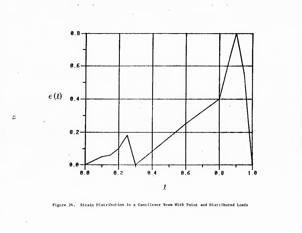
Figure 24. Strain Distribution in a Cantilever Beam With Point and Distributed Loads

e

e'in -5

-10

-15

1 MMMH

•i

m

1.

(.

' 1 t ' 1 1 e.e 0.2 P.4 0.6 0.8 1.0

Figure 25. Shear Diagram of Cantilever Beam in Fig. 24

< t

-0.1

Q(K)

-8.2

-9.3

-8.4

Figure 26. Crosstalk Spectrum of Cantilever Beam with Point and Distributed Loads

*- *>

0(K)

Figure 27. Sine Transform of Q(K)

Improved agreement between the inferred bending strain, as obtained from the

core contrast spectrum, and the true distribution requires further processing.

Only a portion of the spectrum is measured. This is equivalent to convolving the

strain distribution with a sharply peaked weighting function which tends to

smooth out some of the features. The relative height of the peaks in Figure 27

cannot be determined accurately since finer resolution is needed; i.e. a wider

scan in K or ^. It is clear that the maximum height of the line at i = 0.9 is

underestimated. A number of steps can be taken to improve the accuracy of the

computed strain distribution through known inverse filtering methods.

45 (The reverse of this page is blank)

SECTION III

EXPERIMENTAL DEVELOPMENT

1. APPROACH

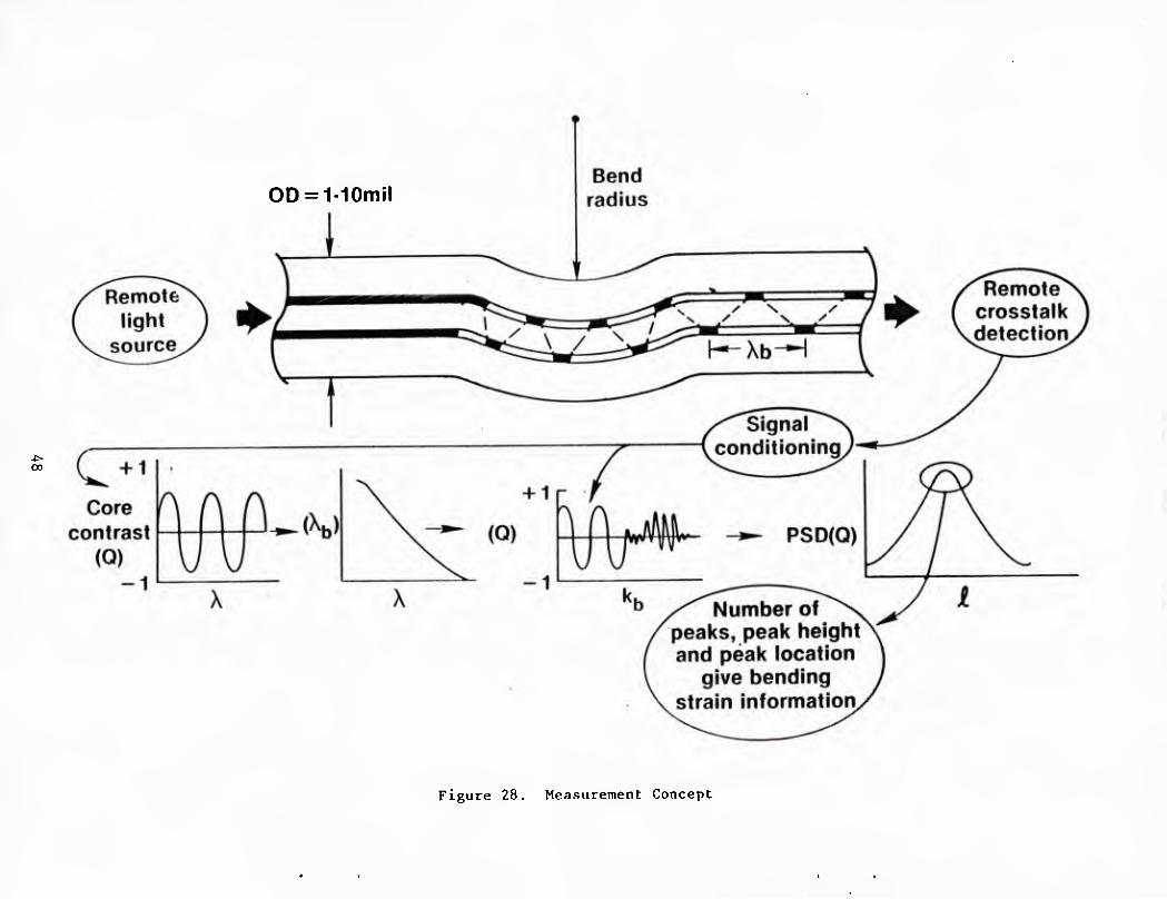
The fundamental measurement and signal processing requirements are shown schematically in Figure 28. The preferred implementation provides excitation of

only the symmetric HEj^ mode such that no crosstalk exists until the sensor is

disturbed. However, due to the close proximity of the two cores and their

intimate coupling, it is difficult to initiate this starting condition. Cross-

talk is typically already in operation at the location of the bend perturbation.

Conceptually, the bend perturbs a portion of the light contained in the symmetric

mode and converts a large portion of the disturbed power into a wave with the

propagation characteristics of the asymmetric mode. Subsequent to this interac-

tion, crosstalk persists with a given beatlength and relative phase to the next

perturbation and/or end of the sensor. Here, the normalized core contrast

function is measured by collecting the power from each core, subtracting them and

then dividing by the sum: (P1-P2)/(P1+P2). This parameter defines Q which is

recorded as a function of the excitation wavelength. When the wavelength scans

through a range of values, Q switches between +1 and -1 in reaction to a result-

ing change in beatlength and phase of the crosstalk function. This provides Q as

a function of the beatlength. When this last function is transformed, it yields

a power spectral density function for interpretation and comparison with the

theoretical calculations. Facilities to implement this approach are reviewed next.

2. APPARATUS

The apparatus for the demonstration experiments is illustrated in Figure 29.

A pulsed dye laser was configured as the variable wavelength excitation source.

Its bandwidth is roughly 0.01 nm which is sufficiently narrow to alleviate

averaging effects during experiments with long sensor lengths (on the order of

one meter long). Typical monochrometers would not have provided sufficient

signal to noise ratio, in addition to imposing a requirement for uselessly short

sensor lengths. Light is transferred to the sensor via a modified microscope.

The twin-core sensor is mounted on a special platform used to impose various

bending configurations. Holders with positioning adjustments were constructed to

permit proper excitiation and constraint without imposing artifacts in the data. These holders represent the fiber termination points before and just after the

bend interaction. The various perturbations, examples of which are identified in

Figure 30, were arranged by placement of several forms and orientation of the

detectors. Identical detectors with integral preamps were separately illuminated

by images of the sensor output cores after dissection by a first-surface

47

4^ 00

OD = 1-10mil

Figure 28. Measurement Concept

♦ I > ^

Dye laser

Detector Preamp Gated integrator Bend

apparatus r-^ A/D converter

4> Computer

Figure 29. Demonstration Experiment: Data Acquisition System

Variable radius Right-angle bend f output

o Input Variable radius loop

Input Output

o

Variable radius Variable spacing Serpentine bend Output

Q Input o

Figure 30. Demonstration Perturbations

splitting wedge. The total energy emitted from the individual cores was measured

for each dye laser pulse by utilization of gated integrator circuits synchronous-

ly locked to the laser trigger generator. A Tektronix digital processing oscil-

loscope provided data previewing functions as well as analog-to-digital conver-

sion for acquisition of the crosstalk signals by the PDP-11 computer. Represen-

tative measurements are discussed in the following sections.

3. PHASE-II DATA AND COMPARISON WITH THEORETICAL MODEL

a. Introduction

An initial set of measurements (Phase-I Data) was conducted with an original

supply of fiber sensors. As work progressed, deficiencies were observed. Much

of the data suffered from low signal-to-noise levels, making it difficult to

detect predicted component peaks in the crosstalk spectrum which were to be

imposed by the perturbations. In addition, many significant, unanticipated

signals were recorded. Such problems made the data difficult to interpret and

nearly impossible to compare directly with the theoretical model as it originally

existed.

These difficulties are not seen as fundamental compromises of the sensor

concept under development in this program. The physics used to formulate the

predictions have a firm foundation. On the other hand, defects were hypothesized

as being associated with the fiber sensor and/or the experimental implementation

causing the measurements to differ from the assumptions used to develop the theory. In addition, the theory required generalization to yield a comprehensive

representation of the predicted results. With these issues at hand, the earlier

results are presented in Appendix A.

Theoretical and experimental improvements described in Appendix B were

implemented to provide an enhanced set of measurements (Phase-II Data) with

corresponding calculations. The tests were conducted on a variety of bends with

geometries similar to those of Phase-I experiments. Every sensor was inspected

to alleviate problems associated with control of dimensions or inclusions.

Mounting procedures were given careful attention, and data was collected with the

new sampling and range parameters. Finally, the calibrated, theoretical model

(upgraded to include dispersion effects) was successfully compared with many of

the measurements.

b. Right Angle Bend

Figure 31 illustrates the crosstalk spectrum measured for a relatively short

sensor subjected to a right angle bend. The same figure compares the predictions

from the new model. The theoretical predictions provide the proper, unperturbed

51

2 in. 2.13 in.

160

120

PSD(Q) 80

40

Straight L = 7.4ln.

0

/ J^

^- ——^ .,,_ <**«;? J„

160

120

PSD(Q) 80

40 1

Bent 2.13 in.

0 0.0504 0.1512 0.252 0

,,l w JiVjWpJ .^^^ ^

0 0.0504 0.1512 0.252

»

1.0 1 0.8 0.6 0.4 1 0.2

/ '.

0 -r T -r -T - -,- f

Frequency (Angstroms-1)

0 0.02 0.04 0.06 0.08 0.10

1.0

0.8

0.6- !\

0.4 /,

.' 1

0.2

0

11/ 1 'v'

"- r—

1

'i.

- T -^— r- '—r- -■ r 1

0 0.02 0.04 0.06 0.08 0.10

Figure 31, Phase II: Short Right Angle Bend. Sample A04.5SQC/ 11.27.29

sensor carrier frequency. The modified spectrum for the bent sensor is also

replicated by the general form of the calculations.

To obtain examples depicting the comprehensive capabilities of the model,

measurements were performed with a much longer sensor. These results are

summarized in Figure 32 for a straight reference case and two bend conditions.

The complexity of the experimentally derived signatures increased when compared

to the measurements with a shorter device. As observed on the undisturbed

carrier frequency, dispersion related effects became more dominant but were quite

well represented in the calculations. Some adjustment of the input conditions for the calculations was required to obtain trends similar to the experimental

results of the perturbed states. The range of adjustments, typically 10 percent,

were reasonable for the current effort. For instance, an important issue arose

with respect to Figure 32 which illustrates the sensitivity of the twin-core

sensor to initial conditions. The center spectral feature could not be computed

without hypothesizing some imbalance (1.2 percent) in the amount of power distri-

buted between the symmetric and asymmetric modes. Such an imbalance could occur

during the experiments if a small amount of excitation energy spilled from the

Airy disk illuminating Core 1 and excited Core 2. This situation might arise if

a small amount of mechanical drift should develop during the measurements or if a

slight defocus of the excitation beam should exist. Standard procedures call for

alignment and focusing checks prior to all measurements, however a slight error

of this type obviously materialized and remained uncompensated. This aspect

would have been difficult to diagnose in the laboratory, yet was easily tested with the model.

c. Single Loop

A bend configured into a complete loop yields a much more difficult test

condition. The crosstalk perturbations become stronger and more complex. Figure

33 is an example which indicates that much fine structure becomes generated in

the crosstalk spectrum. The detailed features appear sensitive to many secondary

aspects of the experiment. This can be illustrated by referring to the theo-

retical predictions. The model calculations contain the important main com-

ponents. For instance, dispersive broadening of the primary carrier is shown along with its shift to a lower frequency after bending. The main feature just

below .05 (1/A) in the measurements is also found in the model. However, the

finer details of the laboratory data above and below this component are not

provided with as much fidelity in the corresponding calculation. All of the

important secondary features exist but not with the proper relative magnitudes.

Finally, small changes in the model parameters yield small, but important changes

as typified by Figure 34. The distributed strain sensing scheme with a twin-core

sensor requires further study to help immunize it from these sensitivities.

A change in core geometry, discussed in the next section, was investigated as a possible variable in this sensitivity issue.

53

0.5 in xH 18.19 In.

1.0 in. ^•117.69 in.

Straight L = 35.13 in

80

Bent

PSD(Q) 40

4S

Q i:v>w4^

0 0.1008 0.2016

80 60 40 20 0

16.19 in.

lOfcC^^H'^bJ^CA: ■fe ̂ ^

0 0.1008 0.2016


80 60 40 20

0

Bent 16.0 In. - -

l\ — - -

■ —

J 1 t .. yv^ \Jl^"W AA/ TM^-

0 0.1008 0.2016

0.8

0.4

0

m 0.8

0.4 I r

0 A

I .■■■ -!—' 1

0.8 • .', 1,

0.4 1

1 (

1 1

1

n j A

-. . , , ,

I S

0 0.05 0.10 0.15 0.20 0 0.05 0.10 0.15 0.20 0 0.05 0.10 0.15 0.20

Figure 32. Phase-II: Long Right Angle Bend. Sample A04.5SQC/ 7 .25 .8 .2

straight L = 30.81 Bent

2.0 in.

-21— 12.12 in. 6.18 in.

80

60

PSD(Q) 40

20

0

;

i t 1

7

1

1 l/ llh H-^vw^v^M^f I'SMIAA--V*

PDS(Q)

1.0

0.8

0.6 0.4

0.2 0

60

40

20

0 0 0.0504 0.1512 0.252 0 0.0504 0.1512 0.252

Frequency (Angstroms -1)

1.0

II

^ -^ - U f- i -1- i Ai T ^ 1 ' r\/f "rs^^^^

PJ

i -"T"

0.8 0.6 0.4

0.2 0

(A ■I

rv'l I T ■'• ■T—r—I"

0 0.05 0.10 0.15 0.20 0 0.05 0.10 0.15 0.20

Figure 33. Phase-II: Single Loop. Sample A04.5SQC/12.18

2.0 in.

80

60

PSD(Q) 40

20

0

Straight = 30.81

I

i ;

1 ■ 4 IK K~ ̂^-v^ (^v f\A T V^/\\^|^^^^^

G) Bent ^^-^^'"- ^-^^ i*^-

PSD(Q)

n

-4] 1

n 7L t- r TjTT^ 1 V

Cv^^Vrr^vr^<-r><V

1.0

0.8 0.6

0.4 0.2

0

60

40

20

0^ 0 0.0504 0.1512 0.252 0 0.0504 0.1512 0.252


1.0

0.8 0.6 0.4 0.2

0

I'll

I !

W

1 I ■

i) h '' I ^ 1,.. 4

, 1 I I II

'ii

0 0.05 0.10 0.15 0.20 0.05 0.10 0.15 0.20

Figure 34. Phase-II: Single Loop. Sample A04.5SQC/12.18

d. Round-Core Sensor

The square-core sensor geometry has been used exclusively in the all major

demonstrations discussed to this point. A square configuration was the primary

subject of interest because of apparent high sensitivity to bending strain

observed in early, qualitative tests. Now, we would like to reduce some of the

sensitivity, so a round-core sensor alternative was investigated. Figure 35 illustrates performance of the round configuration during a right angle bend.

Theoretical modelling of the experiments shows good correlation with the measure-

ments. Furthermore, numerical tests showed no fundamental difference in the

sensitivity of the round-core device when compared with the square geometry.

Therefore, we conclude that other parameter changes must be implemented to alle-

viate the critical nature of the twin-core response to its operating conditions.

57

2.0 in. v'l2.112in.

Straight L = 7.26 Bent 2.048 in.

PSD(Q)

00

120

80

40

0

i

vO^ L u VV --W.. >r>f =pp>» CPCP <s»^

0 0.0504 0.1512 0.252 0 0.0504 0.1512 0.252


1.0

0.8 0.6 0.4

0.2

0

I

0 0.02 0.04 0.06 0.08 0.10

1.0

0.8 0.6 0.4

0.2

0

!\ .' ■■• I

0 0.02 0.04 0.06 0.08 0.10

Figure 35. Phase-II: Right Angle Bend; Round Core. Sample AORDC/12.5.6

SECTION IV

SUMMARY AND RECOMMENDATIONS

This document discloses the investigation of a unique concept for

measurement of distributed strain. Implementation of the technique utilizes a

fiber optic device with twin, coupled cores, a single input and a single output.

Multiple wavelength operation of the sensor yields a diagnosis of the waveguide

coupling perturbations imposed by mechanical disturbances, A general theory for

the device has been derived in the form of an integral equation that connects the

sensor core contrast to an arbitrary bending strain or curvature. In many cases

of interest the curvature is small and slowly varying. For these conditions

theory shows that the crosstalk spectrum is directly related to the Fourier

transform of the strain distribution on a cantilevered beam. This result per-

tains to a wing with gradual bends (radius of curvature large compared to arc

length) while stipulating very practical requirements on potential sensor para-

meters (radius of curvature large compared to device beatlength). The experi-

ments summarized in this report confirm the theoretical predictions.

Two computer models were developed from the theory. One model provides a

rudimentary simulation of a wing (cantilevered beam). It was used to prove that

the Fourier transformation of the simulated sensor output matched the bending

moment distribution. The second model was created to calculate the sensor

response for comparison with the demonstration experiments. Complete spectral distributions were provided. Another important feature of this second model was

that it could be adjusted to match laboratory sensor calibration data for

absolute beatlength and dispersion, thereby improving correlation between theory

and experiment.

Fiber optic devices were designed and fabricated for laboratory-scale

tests. Sensor performance was diagnosed by techniques established in direct

support of these demonstrations. Verification experiments performed with simple

bending perturbations in the laboratory apparatus exhibited complex spectra and

low signal to noise results during Phase-I. In addition, the form of the theory

provided only spectral feature designation, not a complete distribution with

properly registered magnitudes. Both of these issues were resolved during

Phase-II. Finally, the improved sensors and experimental conditions confirmed

the general form of the sensor spectra predicted by the model.

Both the theory and the experiments indicate that the twin-core device is highly sensitive to its mechanical environment and its operating conditions.

Small modifications to the relative power content for the symmetric and asym-

metric modes at the input caused significant changes in the crosstalk spectrum.

Similar results were observed for changes in the form of the beatlength versus

59

wavelength scanning function. The crosstalk spectrum responded in a sensitive

way to changes in the absolute beatlength range and dispersion in the function.

Under most experimental conditions the sensor response was so sensitive and the

measured output so complex that interpretive support by the theoretical model was

essential. We recommend that a new operating regime be identified for further

laboratory investigation. The new conditions must be identified through analytic

and numerical development directed toward desensitizing the experimental devices

and reducing the complexity of their responses. Changes in both the device

parameters and the experimental perturbations are anticipated. Polarization

effects in twin-core sensors should also be investigated.

The basic results of this investigation indicate that the twin-core concept

for measurement of distributed strain is valid. However, practical implementa-

tion with the present sensors is very complex. Further study may yield improved

sensor operating regimes with corresponding simplification of its response. In

conclusion, this fiber optic sensor concept requires additional investigation and

development to optimize device parameters for application to distributed strain

diagnostics for airframe structures.

60

APPENDIX A

PHASE-I DATA

1. INTRODUCTION

This initial set of measurements was conducted with an original supply of

fiber sensors. As work progressed, deficiencies were observed. Much of the data

suffered from low signal-to-noise levels, making it difficult to detect predicted

component peaks in the crosstalk spectrum which were to be imposed by the pertur-

bations. In addition, many significant, unanticipated signals were recorded.

Such problems made the data difficult to interpret and nearly impossible to

compare directly with the theoretical model as it existed at this point.

These difficulties are not seen as fundamental compromises of the sensor

concept under development in this program. The physics used to formulate the

predictions have a firm foundation. On the other hand, defects were hypothesized

as being associated with the fiber sensor and/or the experimental implementation

causing the measurements to differ from the assumptions used to develop the

theory. In addition, the theory required generalization to yield a comprehensive

representation of the predicted results. With these issues at hand, the earlier results are reviewed.

2. UNPERTURBED SENSOR SIGNATURE AND LENGTH SCALING

Figure A-1 provides a graph of the core contrast function which comes from

measuring PI and P2 at the sensor output as the excitation wavelength is scanned.

The result is a sine-wave-like signal. Eventually, structural data will be

interpreted by diagnosing the Fourier Transform of this signature. It is easy to

see that when a spectral analysis (achieved by Fourier Transforming) is performed

that it will consist of one primary frequency peak and miscellaneous other lower

level noise signals. This insight is supported by Figure A-1, with further

indication of the coexistence of a very low frequency signal. This low frequency

feature was not anticipated for a benign sensor condition.

There was concern that the extra, low frequency signal resulted from sensor

deflections imposed by misaligned termination units. Another sensor (Figure A-2)

was tested for this effect. Evidence indicates that the sensor must exit the end

mounts cleanly, without kinks in order to obtain a cleaner spectrum. To further

test this aspect, another sensor, Figure A-3, was subjected to changes after the termination units were carefully adjusted.

To begin with, a very different signature was obtained for this third

device. The low frequency component existed but so did a very complex structure

61

1.0

Core 0.5

contrast 0 (Q)

-0.5 o\

RH \j\j

p^n^o^ do 1 OL/\VJ«/ HXJ

20 ^\J '

J 1

0 L --^ -y/V r \A ̂ ^ 5»?*=>- <:>»v

0 51.2 153.6 655.6

Wavelength(Angstroms)

0 0.0516 0.1547 0.2578


Figure A-1. Response of Straight Fiber. L=100 cm; Sample 4045QC/DSS3.141

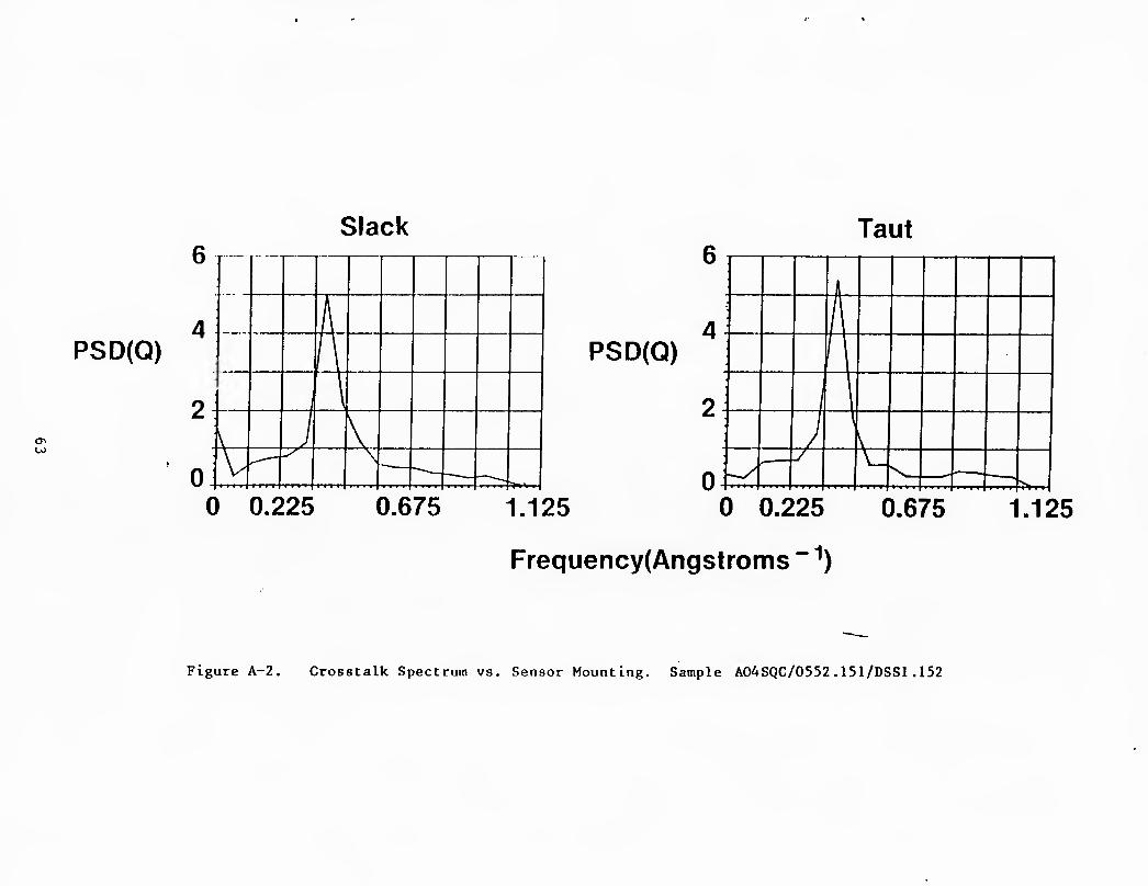
Slack Taut

PSD(Q)

0

Hi PSD(Q)

VJ

A

A A '

2 i £m J \

\

0 J v_

5v^

0 0.225 0.675 1.125

Frequency(Angstroms ^)

0 0.225 0.675 1.125

-^^

Figure A-2. Crosstalk Spectrum vs. Sensor Mounting. Sample AO4SQC/0552.151/DSSl.152

L = 99.21cm L = 91.6cm

60

PSD(Q) 40

20

0

rt

-it ■ itt tit IT

60

40

20

0

n 1 1 lA 1 f\

L f/V^ v*ft: /V^ Y/ k/H :>:«

L — 84.0cm

120

80 J

40 v1

/ \

0 Srfw^ybWJC / V "y.^^^ 0 0.0813 0.1625 0 0.0813 0.1625 0 0.0813 0.1625

0.0406 0.1219 0.2031 0.0406 0.1219 0.2031 0.0406 0.1219 0.2031


Figure A-3. Length Scaling in Crosstalk Spectrum. Sample A04SQC/DSS4.31/D8S4 .51/DSS4.61

around the primary frequency. This type of signature variation could hinder

proper interpretation during more complicated experiments, therefore we attempted

to uncover the reasons behind the extra low frequency component and the appear-

ance of complex features in the vicinity of the primary crosstalk carrier.

The scaling relations of Section II were used to guide the next test. The

theory might lead one to interpret that the multiple peaks in the primary carrier

of Figure A-3a are resulting from a sensor perturbation a few centimeters in from

the sensor output termination. In an attempt to remove whatever type of inherent

perturbation that might exist there (the termination units were well aligned),

7.6 cm were cut from the output end. Figure A-3b shows no substantial change in

the general range of features in the spectrum after removal of the suspected

piece of sensor. So an attempt was made to clip off 7.6 cm from the input end of

the sensor in an attempt to eliminate the low frequency feature. It too would

not disappear. The spectral changes from the earlier test case of Figure A-1 to

the case of Figure A-3 appear to result from some inherent, nonideal characteris-

tic associated with the sensor itself. The defect appears to be distributed over

the entire fiber length and not isolated to the end regions.

Next, length scaling in the crosstalk spectrum was investigated. Section II

predicts that the primary carrier signal, the dominant higher frequency feature

of Figure A-1, should shift position in frequency space in direct proportion with

sensor length. A test of this scaling is presented in Figure A-3. Several

issues become apparent. Even though the quiescent, unperturbed crosstalk

spectrum for this sensor was not identical to that of Figure A-1, the average

location of the carrier peak does respond properly with length reduction. Hence,

a scaling relationship appears verified, but a variability in the shape of the

sensor signature has arisen.

3. RIGHT-ANGLE BEND

The effect of bends on propagation in a fiber can be quite complex. Three

phenomona result for single core fibers: (1) resonant microbend conversion of

energy from one mode to another, (2) nonresonant macrobend induced radiation

losses for constant radii of curvature and (3) extra radiation effects associated

with transitions between regions of constant curvature. For twin-core fibers a

combination of the above could coexist with a fourth aspect: (4) relative phase

shift between modes due to perturbations in core indices of refraction. During

our experiments, we would like to eliminate or minimize the first three aspects.

This is accomplised by limiting the range of perturbations placed on the sensor.

For instance, no significant bend disturbances with short spatial wavelengths

will be applied, therefore no microbend loses will be induced. From Reference

1 we find that if all of our experimental disturbances are associated with radii

of curvature greater than 2 cm, then radiation induced coupling will be

minimized. Finally, Reference 2 indicates that transition effects are of most

concern, but with care these are minimized by not crimping the sensor. In short,

65

we would like to limit the crosstalk inducing aspect of bends to only the inter-

actions described by Section II, which are to be of dominant importance to full-

scale monitoring problems.

Reference data (straight sensor) of Figure A-4 is compared with data from a

twin-core sensor after bending 90 degrees around a form, Figure A-5. The bend

did not appear to impose large signals, so the logarithm(ln) was computed to help

increase the general visibility of potentially important signals. Superposition

of the signal locations predicted for the geometry of the bend (Figure A-5)

indicates the occurrence of information consistent with the theory. But the

results are short of conclusive. Therefore additional measurements were

conducted.

4. SERPENTINE BEND

Two circular forms were used to define a serpentine path for the twin-core

sensor as shown in Figure A-6. Crosstalk spectra were measured as a function of

increasing separation. A, and compared with the straight reference condition.

Figure A-7 supplies logarithmic plots of the PSD. Each case shows a super-

position of the spectral components predicted by the theory in its early form. Once again, signals in the perturbed state are consistent with the model, but

they are not as strong and definite as expected.

5. SINGLE LOOP

The complexity of signals in Section A-2 and the weakness of others in

Sections A-3 and A-4 led us to another experiment. This time, the measurements

were conducted at a single wavelength while the radius of a single loop was

changed. Such an experiment should verify sensor response to this kind of

perturbation. Figure A-8 illustrates strong crosstalk changes when the radius of

the loop changes. In addition, the period of the crosstalk cycle rate versus

radius appears to be monotonically changing. These results lead us to believe

that significant signals should result for fixed perturbations, but with variable

wavelength excitation. Hence further experimental conditions required investi-

gated. Prior to such an extension of the effort, exploratory work was conducted

to facilitate improved signals.

6. DISCUSSION

Measurements reviewed in Sections A-2 through A-5 were investigated during

the first phase of this program. Several problems were discovered. The sensor

response was generally weak, yet very complex and difficult to interpret. Simple comparison with predicted spectral line locations is insufficient. A more

comprehensive interpretation must be made available. In addition, sensor

deficiencies should be investigated in support of more reliable, cleaner and

stronger signatures.

66

♦■ •

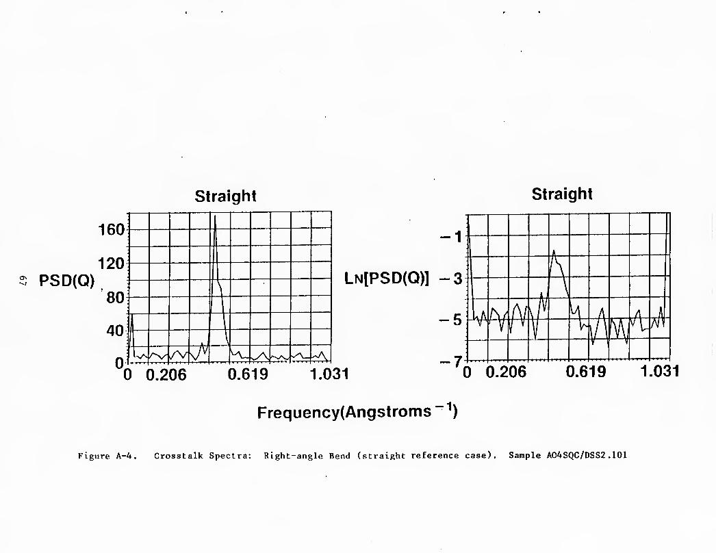
straight Straight

ON PSD(Q)

160

120

80

40

0

■ 1

\

1- 1

A \

L^ K- -y\ u_ ̂

0 0.206 0.619 1.031

-1

LN[PSD(Q)] -3

-5

-7

h

K k 3

■ j^buNxB ^ A,__ A J_ -"ti^ff-f]^ ^M^'^ V ' V

0 0.206 0.619 1.031

Frequency(Angstroms ^)

Figure A-4. Crosstalk Spectra: Right-angle Bend (straight reference case). Sample A04SQC/DSS2.101

CD PSD(Q)

ocn 1 Bent

zoU

onn ZKJVJ

100

50

0

\

^ ^^ Ay \ Iv --yv^ V<:^ ̂ ^ ̂ -%

LN[PSD(Q)1

1

-1

-3

Bent

-7

0 0.206 0.619 1.031 w" f * < * '• w r*

A^

0 0.206 0.619 1.031

-ii Frequency(Angstroms ')

Figure A-5. Crosstalk Spectra: Right-angle Bend (perturbed case). Sample A04SQ/DSS2.81

Output

Figure A-6. Serpentine Demonstration

69

o

straight

LN[PSD(Q)]

LN[PSD(Q)] 1

-1

0

A = 4in.

\ j 1

A; J^ y ^ r u f \l^ AA y V % V vA 1/

:■ ;■

'

: ■*-f-f*

1 0.1031 0.2062

0

-2 0

A = 2i in.

A = 7i in.

\ ^ /

'

/*\ A V 11 \ / 1 ¥

1 \A - y ̂ / ̂ , \A !

f V V r 0.1031 0.2062


Figure A-7. Crosswalk Spectra: Serpentine Bend. Samples A04SQC/ DSS3.141/DSS3.15/DSS3.201

Q

0.8 0.9 1.0 1.1 1.2 1.3 Loop radius (inches)

Figure A-8. Crosstalk vs. Loop Radius. Fixed Wavelength = 6328A. Sample A04SQC/DSS7.00

71

Problems were discovered in many facets of this initial effort. There were

some manufacturing defects which caused a variation in the sensor diameter as a

function of length, as well as bubble inclusions. These issues induced deviation

of the sensor signals from predicted response. Finally, changes in the sampling

range and intervals along with special signal processing were expected to improve

matters significantly. Investigation of these issues is presented in Appendix

B.

72

APPENDIX B

IMPROVEMENTS

1. INTRODUCTION

The complexity and indecisive character of the preceding data compared with

the simplicity of the theoretical predictions led us to re-evaluate our experi-

mental apparatus, sensors and our modelling approach. This section describes

improvements which were tested, in addition to discussing some deficiencies which

were uncovered and rectified.

2. SENSOR QUALITY

The issue at hand is why does the theoretical description of a somewhat

limited sensor, yet perfect within its assumptions, not match the response of the

sensors used in the measurements. It is possible that the quality of the real

sensor was insufficient for replication of the predicted signals. Since this

investigation is concerned with a totally new concept, parameters concerned with

intrinsic sensor quality must be interpreted from experimental difficulties or

derived from theoretical descriptions. For instance, if the two sensor cores are

not perfect mirror images of one another, then coupling diminishes rapidly. Such

a geometric mismatch could lead to major discrepancies between the experimental

and theoretical results. On the other hand, this problem is not of major

importance in our case. The scanning electron micrographs of Figure B-1 show

excellent core-to-core symmetry. However, another problem could develop.

Practical crosstalk coupling coefficients could differ from the theoretical model

if the outside diameter is not consistent from sensor beginning to end; even

though at each point along the sensor, the cores are twinned. Such a problem

would lead to individual sensor sections interacting with distributed bends while

exhibiting a variable beatlength. The original theoretical model does not allow

for such a sensor variation, assuming that only one geometrical operating condi-

tion of Figure B-2 is effective for the entire length. Review of sensor material

utilized during the demonstrations of Sections A-2 and A-5 indicate a peak to

peak size fluctuation of 22 percent—very significant, depending on the excita-

tion wavelength. This level of variation could lead to major discrepancies

between the measurements and the predictions. Under the improved form of the

experiments, new sensors were procured, yielding signficantly improved dimen-

sional control, only 7 percent peak-to-peak fluctuation. The quality of the

sensor crosstalk response demonstrated a corresponding improvement (Figure B-3).

Most significantly, the basic crosstalk signal-to-noise ratio appears improved by

at least a factor of 50 and under special conditions as much as 200.

Any characteristic which might disturb the crosstalk function in magnitude, phase or frequency was considered suspect. -The older sensor material showed

73

12,000 X 2.63/im

4>

HBj^, ," Y Jt '^^1

,'■■ ,.:-\'

■■'■^■■■■■■■'- ■

■-••■, ,' ,i

^ ^.63/(rTp .47/trn'

12,000 X 2.15/im

Fiber 0D = 114/(m

2.12/tm 2.28/(m

Fiber OD = 109/(m

Figure B-1. Twin-Core Geometry

^1

Beatlength (Xb, mm)

0.6 0.8 1.0 1.2 1.4 1.6 1.8 2.0 2.2 Core dimension (a,/xm)

I 1 L__^ I I I 11 102 128 153

Sensor OD (D, \ivc\)

Figure B-2. Beat Length of Original Square Core

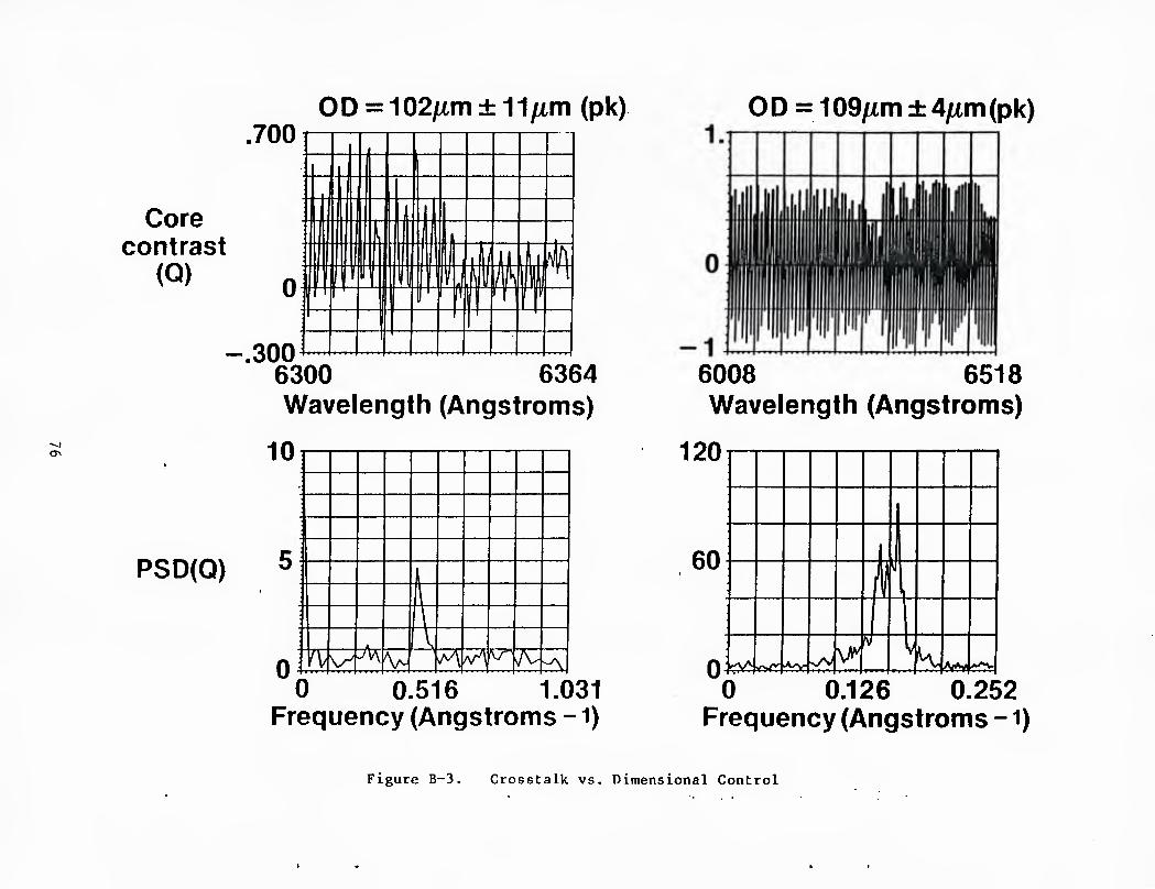
.700 OD = 102/im±11/xm (pk)

ON

Core contrast

(Q) 0

-.300

1

I ,

ilL- I 4-^ nffi

^ ll ^ l''l "i I ^tW 1 1 r IP rT Vf' ^ ^ i 1

6300 6364 Wavelength (Angstroms)

PSD(Q) 1

\ '

A \

TVv^^ V V^ A^ ̂ r' A- -A 0 0.516 1.031


O D = 109 fim ± Afim (pk)


iiU-

60 1 1 1

0 krV>U<4^ vA/ V^ M V

v^^f<v<<>

0 0.126 0.252 Frequency (Angstroms -1)

Figure B-3. Crosstalk vs. Dimensional Control

many strong scattering centers when illuminated by the dye laser. These

inclusions could scatter light from the normally crosstalking cores, causing two possible side effects: a wavelength dependent reduction in core contrast and an

initiation of extraneous crosstalking uncorrelated with the primary bend

function. In either case the sensor output could be significantly disturbed from

predictions. This type of internal defect existed in some of the new sensors

procured for the extended program, but pretest inspection enabled selection of

material visually free of scattering problems. Signal improvements such as those

demonstrated in Figure B-4 resulted from the inspection/control effort.

Finally, the model was based on a specific core orientation relative to the

plane of the bending perturbations. A twist of a few degrees per cm in the core

orientation was discovered in the original material. For long devices utilized

for these experiments this defect is significant. The issue was corrected in the

new sensors by taking more care in preform fabrication and fiber drawing

methods.

3. APPARATUS MODIFICATION

The previous section dealt with sensor associated problems. However, we

observed the need for improvements in the experimental apparatus (Figure B-4).

More specifically, the sensor end fixturing was of most concern. The original

termination approach provided a short section of capillary tubing in which the

sensor ends were secured. These tubing sections were then placed in differential

positioners. Each piece of termination tubing was from 2 to 4 inches long. If

the axis of the input and output mounting tubes were not properly aligned, then a

kink would develop near the ends of the sensor route. Measurements indicated

that this degraded the data. The problem was cured for the extended program by

fabricating special tubing fixtures which held the sensor by the very first and

last l/8th inch of material, mitigating interfering responses.

4. SINGLE MODE EXCITATION

Section II predicts that the sensor output signals will become simplified and will increase in strength when operation is initiated through excitation of

the symmetric mode, exclusively. We attempted to utilize this advantage during

the improved experiments. There are two obvious methods to achieve this launch

condition: (a) excite with illumination which initiates only the symmetric mode,

or (b) taper the fiber input to fabricate a filter against the asymmetric mode

while utilizing the normal illumination. Both have been tried. To begin with we

attempted to start propagation with strictly the symmetric mode without size

modification to the sensor. Expanded beams were used to provide good approximations to the required equal-amplitude/equal-phase illumination. Some rejection

of the asymmetric mode was noted, but crosstalk in the quiescent sensor was still

dominant. Since this approach did not adquately discriminate against the

asymmetric mode, we tested the mode filtering ability of a tapered input section

on the sensor.

77

Scattering defects; inferior mounting

Core contrast

(Q)

•SI Ob

6175 6190

1 0.8

Core 0-4 contrast Q

-0.41

- 0.8 -1

Scattering defects; improved mounting

6175

1

Core 0.5 contrast

(Q) -0.5

No scattering defects and improved mounting

0

n f \ 1 \ T \ 1 1

\ 1

V \

1 \ 1 \ J 1/ -1


6206

Figure B-4. Crosstalk Improvement Comparison

Initially, it was necessary to document the approximate size and operating

wavelength at which the filtering condition becomes active. The effect is

clearly shown in Figure B-5 for a sensor of uniform diameter: at a sufficiently

long wavelength, the asymmetric mode is discriminated against, and crosstalk

cannot exist. A more comprehensive picture of the onset of the filtering action

is provided by Figure B-6 which plots the relative magnitude of the crosstalk function versus excitation wavelength. To test full implementation of this

concept, the input end of a twin-core sensor was tapered to a size smaller than

the remaining fiber. For wavelengths longer than the cutoff value, this reduced

sensor section should not allow propagation of the asymmetric mode. Therefore,

only the pure symmetric mode should enter the active section of the sensor. The

test consisted of measuring core contrast at the device output as a function of

wavelength. If the asymmetric mode was effectively suppressed by the input

filter section, then crosstalk would cease beyond some critical wavelength. This

type of response could not be detected. To check the performance of the filter

section, the sensor was reversed; the taper at the output. With this orienta-

tion, filtering action was observed as shown in Figure B-7. Therefore, the

filtering concept appears valid but the implementation requires more investiga-

tion. We believe that the taper must be slower, in fact, sufficiently slow to be

classified as adiabatic. This condition can exist only for tapers which are many

beatlengths long. The example of Figure B-7 appears to suggest a taper longer

than 5-10 beatlengths is required. When this is achieved, the new excitation method may work and yield improved signals.

5. MEASUREMENT PARAMETERS AND SIGNAL PROCESSING

The wavelength range and sampling interval used during data acquisition are

important for this research because of the characteristics of the sensor reliance

on a Fourier transform interpretation of the signals. The total wavelength range for sensor operation exists from the asymmetric mode cutoff wavelength (V=1.2) to

the wavelength at which the cores allow higher-order mode propagation (V=2.4). On the other hand, the number of samples is ultimately determined by the

bandwidth of the dye laser (0.01 nm), defining the number of unique samples which

can be made within the total range. From a practical point of view, however,

computer storage and data processing time set the limits during these experi-

ments. The laboratory computer could not efficiently handle data arrays larger

than 256, therefore all measurements consisted of sample sets smaller than this.

While experimenting with the actual number of samples per measurement array, it

was discovered that the twin-core sensors exhibited a dispersive effect, that is, the beatlength was not a linear function of the operating wavelength. This fact

affects the appearance of the data and imposes a coordinate transformation on the

Fourier analyzed data, somewhat complicating the signatures interpretation. The

dispersion is illustrated by making measurements with a fixed interval but with

increasing range (Figure B-8). The dispersion problem is addressed later in Section A-5.

79

00 o

Relative crosstalk

magnitude (Q)

I

Xj = 5236 \ = 5299

(X, = 5500 f \ = 5691

/V'"^-^

|X., = 5984 I \ = 6047

Wavelength intervals (A)

Figure B-5. Crosstalk Near Asymmetric Mode Cut Off

Relative magnitude

of crosstalk

5.5

Wavelength (x 10/im)

Figure B-6. Asymmetric Mode Filter. L = 30.8 inches; O.D. = 61 ym. Sample A02.ASQC/8.29

81

15 Sensor -12

diameter g

Filter/sensor geometry

10 (ixm)

0

3..:;:::;:::

•»MB»*»»<

-t——t ■ I « I ■ I I > ■ t ■ I ■ I ■ I I I I I I I

0 4 8 12 16 20 24 28 Sensor length (inches)

00 to

In

0.800

0.400 Core

contrast (Q)

- 0.400

0

- 0.8001

y^ Out In

Core contrast

(Q)

0.260

0.280

0.300

0.320

0.340

0.360:

£

Wavelength

^\^ ,/" Out

• 99'v\tWW'W f t'T-* t|t»IF»|*y

m Wavelength

64

Figure B-7. Asymmetric Mode Filter

Range = 6008 A to 6136 A

80

AX = 2 A

60

PSD(Q) 40

20

00

Range = 6008A to 6261 A 90

70

PSD (Q) 50

30

10 0

1 1

- . - 1 '

/ An .^ *5<5 ♦CW? <>«< -V / T n.

^0 0.0413 0.1031 0.2062 ^0 0.0406 0.1016 0.2031 Frequency (Angstroms-1) Range = 6008A to 6520 A 80

60

PSD(Q) 40

20

0^ 0 0.0504 0.126 0.252


i 1 f 1 I|

I P A

VM -v^ A. W ■^

^ i\ S-v

Figure B-8. Parameter Assessment: Straight fiber. Sample A045SQ/DSS7.191

After improving the data collection parameters (range and sampling period)

and acquiring new information, there are numerous methods which can be applied

for interpretative post-processing. In order to define a processing sequence,

one must select a specific parameter in the signatures to be optimized and

identify whether or not decision-making processes must be implemented. For

example, one immediate improvement incorporated for each measurement was subtrac-

tion of the mean array value from measured crosstalk signals. This step reduces

the appearance of somewhat useless DC offsets which can show up in baseband

region of the spectra. The next problem pertains to clarifying the existence of

important spectral signals. In the case at hand, low level bend-induced signals

must be detected. These signals should appear in the crosstalk spectrum with

various magnitudes and locations indicative of the perturbations placed on the

sensor. In addition, the primary carrier component is expected to be significant

in all of the demonstrations. If the weaker bend-induced signals result from

geometries causing them to fall adjacent the sensor total-length signal, then

interferences may exist. Sidelobes associated with the stronger signal may over-

lap or obscure bend-induced signals. Signal processing methods which might

reduce some of this interaction could enhance our basic spectral interpreta- tions.

Sidelobes exist as artifacts of the discrete sampling process utilized over

the fixed bandwidth of the finite Fourier Transform. The parameters of sampling

period and total sample array width are represented by the dye laser measurements

at fixed wavelength intervals over the selected operating range. In the Phase-I

data, the spectrum was calculated by taking the Fourier transform of the cross-

talk array as sampled. In such a situation the spectrum consists of a signal

array with many individual elements. Some features contained in this signal

array are not related to the crosstalk data but are related to the parameters of

the Fourier transform. Manipulation of the ancillary features may improve the

clarity with which signals can be detected. For instance. Figure B-9 shows the

ideal spectral form that a single, perfect crosstalk cosine function would

exhibit when the finite Fourier transform is performed over a crosstalk array of

unity magnitude. The original array was greatly padded. The term padding refers

to the addition of many zero-magnitude array elements to the crosstalk data

before it is transformed (see Figure B-10). This process provides optimized

interpolation in transform plane, allowing the signal sidebands to be plotted

with great detail. If the transform is performed strictly over the data array

without padding, then the spectrum will yield only an outline of Figure B-9 by

approximately connecting the peaks of the sidelobes and dissolving the detailed

features. In either case, it is obvious that a second signal feature falling

adjacent the original would cause a complicated interaction which might leave

both indistinguishable. To combat this problem, a method can be utilized to

reduce the strength of the sidelobes and therefore reduce their potential inter-

fences. This can be accomplished by applying carefully tailored windows to the

crosstalk data array prior to tranformation. The implementation of this window-

ing process is conceptualized in Figure B-ll» Several candidate window functions

84

00

Fourier transform

magnitude, dB

-90-

0 0.0502 0.1004 0.1506 0.2008 0.251 0.0251 0.0753 0.1255 0.1757 0.2259

Angstroms-1

Figure B-9. Signal Processing: Rectangular Window Response

Crosstalk data array 1

PSD(Q) "Outline" of function

00

Padded array

Q' 0

-1 W PSD(Q')

Interpolation which

yields complete function

Figure B-10. Signal Processing: Concept of Padding Crosstalk Array

Crosstalk data array

00

Q

W

QxW 0

-1

Figure B-11. Signal Processing: Concept of Windowed Crosstalk Array

are shown in Figure B-12 and their effects on a single frequency cosine signal

plotted in Figures B-13 through B-16. The performance of these window functions

is defined by their relative ability to reject sidelobe effects while not

spreading the main signal lobe. If the window broadens the primary signal

feature too much, then resolution becomes compromised. A performance comparison

is provided by Table B-1 where the sidelobe rejection levels and resolution

widths are summarized (interpreted directly from graphs rather than detailed

calculations). We have selected use of the Kaiser-Bessel window as the best

combination of good sidelobe rejection while maintaining high resolution. Application examples will be presented later in this section.

We tested other signal processing steps which were related to making a

comparison or decision about the perturbed sensor relative to the straight

reference case. Such processes will aide our evaluation of the distributed

sensing technique and the complexity of its application. The steps appear in

Figure B-17, which highlights normalization, ratioing and thresholding opera-

tions. To develop several test cases, we.subjected some of the Phase-I data to the processing philosophy.

Excellent qxialitative improvements were demonstrated through the implementation of the extra data manipulation. Linear signal presentation becomes less

cluttered and easier to interpret. In fact, as seen in Figure B-18, it might be

preferred over the logarithmic plots when signal levels are strong enough. But

if weak and strong signals must be compared on the same graph (Figures B-19 and

B-20), the logarithmic presentation helps greatly. The threshold process, as a

yes/no detection indicator of spectral features, shows good potential even though

more development is required. Thresholds other than unity must be developed,

based on the statistical characteristics of the signals and the type of decision-

making desired. Unfortunately, there are still unclear situations in which

either signals are missing or unexpected signals have appeared. From a decision-

making point of view, this type of error leads to some misses and false-alarms.

Furthermore, the model does not provide the relative magnitude of signals—only

location. Therefore, one cannot develop a complete predicted picture of the

crosstalk spectrum. This deficiency has been rectified during the improvement phase of our work and is demonstrated with the Phase-II data.

After reviewing the raw and the processed signal comparisons, it appears

that some other problem remains. Correlation between the model and the experi-

ments requires improvement in order to provide more definitive results. One

important issue which addresses this problem is discussed in the next section: calibration of the model to the laboratory sensors.

6. SENSOR CALIBRATION MEASUREMENTS

In preceding discussions, we demonstrated improved techniques for inter-

preting the experimental measurements. Discrepancies still exist. In an attempt

00 v£>

w

w

1

0.8

0.6

0.4

0.2

0

Kaiser-Bessel window

/

/ \ \

/ \

/ \

/

/ s k y

/ \

V

Dolph-Chebyshev window 1

0.8

0.6

0.4 0.2

0

> / \

i

/ \

1 / \

\

: / \

'_^ / V ̂ ^

0 25.6 51.2 76.8 102.4 128 Array element

3-term Blackman-Harris window 1

0.8 0.6 0.4 0.2

0

V N

I fr I |t»»i |>T»'Tffyft|» I'T'^yitttf »»TT |rrtt|i>fT't*^<

4-term Blackman-IHarris window 1

0.8 0.6 0.4 0.2

0

/\ 1 \ 1 \ ■ J \

- ■■IT- ^.

/ \ X

0 25.8 51.6 77.4103.2129 Array element

Figure B-12. Signal Processing: Candidate Window Functions

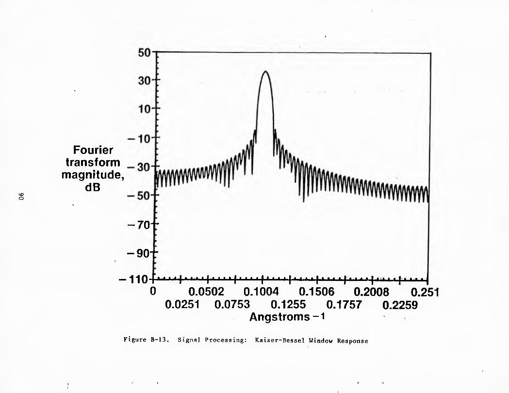
o

Fourier transform

magnitude, dB

-70-:

-90-:

—"HO r*'' * I * * * * I'''' f *' *' I * * *' I *' * * I'' * * j *' ^ * i'''' I'''' I 0 0.0502 0.1004 0.1506 0.2008 0.251

0.0251 0.0753 0.1255 0.1757 0.2259 Angstroms-1

Figure B-13. Signal Processing: Kaiser-Bessel Window Response

Fourier transform

magnitude, dB

-90

0 0.0502 0.1004 0.1506 0.2008 0.251 0.0251 0.0753 0.1255 0.1757 0.2259

Angstroms-1

Figure B-14. Signal Processing: Dolph-Chebyshev Window Response

Fourier transform

magnitude, dB

-70

-90 -

_ -fl •jQ,'iiiijitii|iiii|ii»»|ii«tj>ii.il»i«i|it.ill»iiiliii»

0 0.0502 0.1004 0.1506 0.2008 0.251 0.0251 0.0753 0.1255 0.1757 0.2259

Angstroms-1

Figure B-15. Signal Processing: 3-Terin Blackman-Harris Window Response

Fourier transform

magnitude, dB

-90

0 0.0502 0.1004 0.1506 0.2008 0.251 0.0251 0.0753 0.1255 0.1757 0.2259

Angstroms-1

Figure B-16. Signal Processing: 4-Term Blackman-Harris Window Response

TABLE B-1. RELATIVE WINDOW PERFORMANCE

Sinewave Results

Window

Blackman-Harris

4 Term 3 Term

Kaiser-Bessel

a = 3.5

Dolph - Chebyshev

a = 4.0

Rectangle

Sidelobe Level (-dB)

93 70

63

72

14

6 dB Width

xlQ-^ A

9.2

7.0

7.7

6.4

94

Original

Experimental apparatus

FFT (Q) vs X

T LOG FFT (Q) ^

LOG FFT (Q,e,) "^ ^

I Threshold ' LOG FFT (Q) | x mresnom , LOG FFT (Q,ef) ( ^^ ^

Improved

Subtract mean Q = Q - Q^VE

T Impose

K-B window Q' vsX

I Pad x4 Q" vs X

FFT (Q") vs X

I Normalize FFT (Q")

i LOG FFT (0") ^

LOG FFT (Q'Vef)

I Threshold LOG FFT (0") , X

LOG FFT (C'ref)'

Figure B-17. Signal Processing Application

40

30 PSD(Q")

PSD(Q'Vef)20

10

Linear ratio

0

1 1 ^

4_-l I

- -T- I ■- ! - 1 1 1

Predicted signal locations

—

|. J 4

1 1 '

'il 1 m^^^ ,-^v\.

Logarithmic ratio T—I—I—I—I—r

j Predicted signal locations

Log[PSD(Q")]

Log[PSD(Q",ef)l 0

-20

0 0.0502 0.1506 0.251 0 0.0502 0.1255 0.251 Frequency (Angstroms-1)

Unity threshold

1

T 0.6

0.2

... 1 1 1 i 1 1

Predicted siqna 1 locations

•: ;

-^»'*T*'l''* _ , ...

■

■ j;;

^ i *

— .._

-1'*^

0 0.0502 0.1255 0.251 Frequency (Angstroms-1)

Figure B-18. Right-Angle Bend Data (Fig. A-5). Processed

Linear ratio

PSD(Q")

PSD(Q'Vef)

160

120

80

40

T—r

_.i

-4-

Q |,,^,4.Mc^

u

Predicted signal

locations

A. M U

Predicted signal "^

locations 40

Logarithmic ratio

Log [P$D(Q")1

Log [PSD(Q'Ve,)]

0 0.502 0.1506 0.251 0 0.0502 0.1506 0.251 Frequency (Angstroms-1)

Unity threshoid

1.2 "7 1 1 1 1 1


0 0.0502 0.1506 0.251 Frequency (Angstroms-1)

Figure B-19. Serpentine Bend Data (A=2 in.; Fig. A-7). Processed

Linear ratio

PSD(Q")

PSD(Q'Vef)

40

30

20

10

Logarithmic ratio

0

, ^__

1^ ■i' ill

i|i Predicted signal ]!; locations

1 li 1 nil 1 1 III •1

II

I'l' •'■I

1 ii>> ijiii

li 11 n II II II ,

A u i/l ̂^i y J _^^ l[ \~


Log[PSD(Q")]

Log[PSD(Q'Vef)l -20

-40^

00

0 0.0502 0.1506 0.251 0 0.0502 0.1506 Frequency (Angstroms -1)

Unity threshold

1.2

0.8

0.251

0.4

•-

■ I I ! 1 I 1 I

Predicted signal d

1 ■ etections

1 1 1 L _ '

J X*.'

MMV' M-L 0 0 0.502 0.1506 0.251


Figure B-20. Serpentine Bend Data (A=7 in.; Fig. A-7). Processed

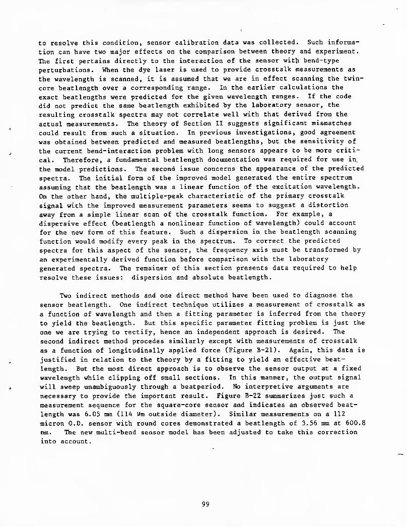
--•7^-'»jr-

to resolve this condition, sensor calibration data was collected. Such informa-

tion can have two major effects on the comparison between theory and experiment.

The first pertains directly to the interaction of the sensor with bend-type

perturbations. When the dye laser is used to provide crosstalk measurements as

the wavelength is scanned, it is assumed that we are in effect scanning the twin-

core beatlength over a corresponding range. In the earlier calculations the

exact beatlengths were predicted for the given wavelength ranges. If the code did not predict the same beatlength exhibited by the laboratory sensor, the

resulting crosstalk spectra may not correlate well with that derived from the

actual measurements. The theory of Section II suggests significant mismatches

could result from such a situation. In previous investigations, good agreement

was obtained between predicted and measured beatlengths, but the sensitivity of

the current bend-interaction problem with long sensors appears to be more criti-

cal. Therefore, a fundamental beatlength documentation was required for use in.

the model predictions. The second issue concerns the appearance of the predicted

spectra. The initial form of the improved model generated the entire spectrum

assuming that the beatlength was a linear function of the excitation wavelength.

On the other hand, the multiple-peak characteristic of the primary crosstalk

signal with the improved measurement parameters seems to suggest a distortion

away from a simple linear scan of the crosstalk function. For example, a

dispersive effect (beatlength a nonlinear function of wavelength) could account

for the new form of this feature. Such a dispersion in the beatlength scanning

function would modify every peak in the spectrum. To correct the predicted

spectra for this aspect of the sensor, the frequency axis must be transformed by

an experimentally derived function before comparison with the laboratory

generated spectra. The remainer of this section presents data required to help

resolve these issues: dispersion and absolute beatlength.

Two indirect methods and one direct method have been used to diagnose the

sensor beatlength. One indirect technique utilizes a measurement of crosstalk as

a function of wavelength and then a fitting parameter is inferred from the theory

to yield the beatlength. But this specific parameter fitting problem is just the

one we are trying to rectify, hence an independent approach is desired. The

second indirect method procedes similarly except with measurements of crosstalk

as a function of longitudinally applied force (Figure B-21). Again, this data is

justified in relation to the theory by a fitting to yield an effective beat-

length. But the most direct approach is to observe the sensor output at a fixed

wavelength while clipping off small sections. In this manner, the output signal

will sweep unambiguously through a beatperiod. No interpretive arguments are

necessary to provide the important result. Figure B-22 summarizes just such a

measurement sequence for the square-core sensor and indicates an observed beat-

length was 6.05 mm (114 Vm outside diameter). Similar measurements on a 112 micron O.D. sensor with round cores demonstrated a beatlength of 3.56 mm at 600.8

nm. The new multi-bend sensor model has been adjusted to take this correction

into account.

99

1

Core contrast

(Q) 1

\

I < I 11 lirNi

3"^ I * I I » » I

■^

-1

Force (102 grams)

Figure B-21. Sensor Calibration: Force Response. Sample

A04.55Q, X=633 nm, O.D. = 0.0045 inch, Lg^=34.204, L.J. = 46.3 cm

100

Core contrast

(Q)

1

512

-1

\ \

s .

1 «***«»■>»» ^ ♦«'■** \ ♦■^■^ 4«* '#»l<<l»t< ■». 4-»-» I* I

\ :\: :;■../:

■/

■j- ■

5.6

(inches)

Figure B-22. Sensor Calibration: Length Change Response: Sample A04.55Q, X=600.8 nm, O.D.=0.0045 inch

101

Characterizing the dispersion, or nonlinearity, in wavelength dependence of

the beatlength requires extensive analysis of the crosstalk data. The non-

linearity is expected to be small but significant to our sensor interpretation so

adequate care must be used in the processing. To begin with, crosstalk is

measured as a function of wavelength for the sensor in a neutral, straight state

(Figure B-23). Two hundred and fifty-six (256) samples were acquired at equal

intervals between 600.8 nm and 651.8 nm. This data array provides samples of a

more complete function. To create our best guess of this function, we utilize an

interpolation technique with a cubic spline fitting routine to provide 12 times

as many array elements. Then, the maxima and minima are detected as a function

of wavelength change. This yields the curve of Figure B-23, crosstalk phase

versus wavelength, which must be diagnosed for nonlinearity. Table B-2 indicates

only small deviation from linear, but as evidenced in Section III, this

correction significantly modifies the shape of spectral features for long sensors

or for broad sample ranges.

102

o

1

0.6

Core 0.2 contrast 0

(Q) - 02

-0.6

15

Crosstalk 10 phase

(0-^1O7r) 5

0 0 100 200

102.4 307.2 512

Wavelength (angstroms)

Wavelength (A -^2)

Figure B-23. X„ vs X Dispersion: Straight Sensor. Sample A04.55Q, L=35.5 inches

TABLE B-2. EXPERIMENTAL DISPERSION EQUATION

Quadratic Fit Parameters

Y=A+Bx+Cx^

A = -3.62 X 10-^

B = 5.47 X 10-2

C = 2.18 X 10-^

Coefficient of Determination = 0.999996122

Coefficient of Correlation = 0.999998061

Linear Fit Parameters

Y = A + Bx

A = -2.35 X 10"^

B = 6.01 X 10-2

C of D = 0.999473001

C of C = 0.999736466

104

REFERENCES

1. Synder, A. W. and J. D. Love: Optical Waveguide Theory. Chapman and Hall, New York, p. 392 (1983).

2. Meltz, G., J. R. Dunphy, W. W. Moray and E. Snitzer: Cross-Talk Fiber-Optic Temperature Sensor. Appl. Optics 22: 464 (February 1983).

3. Murakami, Y.: Appl. Optics, 19: 398 (1980).

4. Murakami, Y. and S. Sudo: Coupling Characteristics Measurements Between Curved Waveguide Using a Two-Core Fiber Coupler. Appl. Optics 20: 417 (1981).

5. Keller, H. B. and J. B. Keller: Exponential-Like Solutions of Systems of Liner Ordinary Differential Equations. J. Soc. Induced Appl. Math, 10: 246 (1962).

6. Ganthmacher, F. R.: Theory of Matrices, Vol. 2, Chelsea, New York, pp. 125- 141 (1954).

7. Smith, R. B.: Analytical Solutions for Linearly Tapered Directional Couplers. J. Opt. Soc. Am. 66:892 (1976).

8. Chen, Y. S. and A. Ishimaru: Proc. IEEE (Lett.) 54, 1071 (1966).

105

(The reverse o£ this page is blank)

U221737

SECURITY CLASSIFICATION OF THIS PAG = REPORT …AFATL/DLCM 9. PROCUREMENT INSTRUMENT IDENTIFICATION...

Documents

Transcript of SECURITY CLASSIFICATION OF THIS PAG = REPORT …AFATL/DLCM 9. PROCUREMENT INSTRUMENT IDENTIFICATION...