Securitization and Heterogeneous-BeliefBubbles with Collateral Constraints

Jun Maekawa

Abstract

Earlier studies have showed that the asset price is higher in a het-erogeneous model than in a common prior model . These studieshave assumed that there is neither budget constraint nor limitation offinancial market. Recent studies have also explored the role of finan-cial technology in heterogeneous belief model. In this paper, I showthat some financial technology including securitization, particularlyloan backed security, increases the asset price as reported by previousstudies.

1 Background

There is a close relation between financial innovations like leverage, securiti-zation or MBS, and bubbles. (Brunnermeier and Oehmke(2013) [2]). In fact,the size of financial innovation grew in recent U.S. crisis. The market of thesecuritization grew during the housing boom, which in their peak amountedto trillions of dollars a year. After the peak of the price in early 2006, theprice declined.Fostel and Geanakoplos (2012) [5] provide models in which different financialinnovations affect the economic situation. Financial innovation like tranch-ing, one of a securitization technology, raises asset prices by increasing theability of the optimist. By tranching, optimists can take riskier positions inthe asset. At the same time, an unexpected introduction of credit defaultswaps (CDS) can lead to drastic reductions in asset prices, since it allowspessimists to more effectively bet against the bubble asset.In the present study, I have showed that financial innovations improve thebudget constraints of traders. The proposed model explain a theoretical

1

framework between bubbles and financial innovations. By the innovation, itis possible for the traders to have enough cash for buying the asset. I havealso showed that innovations increase the market instability, such as bubbles.I also explained the relation between asset prices and financial technologies.Harrison and Kreps (1978) [9] described heterogeneous belief bubbles . Theyreported that in their model, the traders ’beliefs change over time. Theprice of the asset can be higher than the valuation of the most optimisticagent.Geanakoplos (2010) [6] develops a model in which agents with heterogeneousbeliefs have limited wealth, such that agents with optimistic views about anasset borrow funds from more pessimistic agents, with loan contracts withcollateral. Because pessimistic agents have lower evaluation about the assetreturn, their finances to optimistic agents are not enough for the optimisticbelief. In this model, optimists tend to make risky investment. When lowasset return states are realized, optimists lose their wealth and more of theasset has to be held by pessimists, The asset price must be affected not onlyby the optimistic belief but also by the pessimistic belief and it is lower thanthat of Harrison and Kreps.Simsek (2013) [15] shows a similar result in Geanakoplos in their heteroge-neous model. He focused on the belief disagreement between optimists andpessimists. The extent to which pessimists are willing to finance asset pur-chases by optimists depends on a specific form of the belief disagreement.Intuitively speaking, when disagreement is mostly about the upside, pes-simists are more willing to provide credit than when disagreement is aboutthe downside. Hence, it is not just the amount of disagreement, but also thenature of disagreement among agents that matters for asset prices.In this paper, I introduced the collateral loan model like Simsek . The assetprice gets higher again and heterogeneous belief bubbles re-arise.There are two original factors, loan securitizations and new optimists.Lenders can sell loan payments to other traders by securitizations. Loanlenders can shift default risks of loan contracts to other traders. As a result,speculative lending occur in equilibrium. In my proposed model, new opti-mists come daily to buy the security issued by the loan lenders. The assetprice is raised by their optimistic trades.Though new optimists have little cash, their cash is indirectly used for buy-ing the asset by the securitization. The loan contract can be securitized andnew optimists buy the security. For the securitization, the lender of the loanhas speculative incentive for lending cash. The borrower can have large cash

2

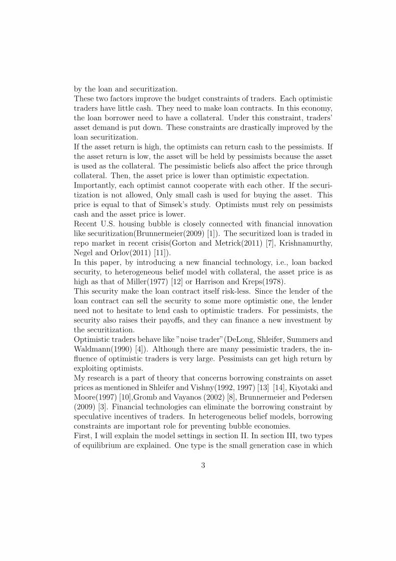
by the loan and securitization.These two factors improve the budget constraints of traders. Each optimistictraders have little cash. They need to make loan contracts. In this economy,the loan borrower need to have a collateral. Under this constraint, traders’asset demand is put down. These constraints are drastically improved by theloan securitization.If the asset return is high, the optimists can return cash to the pessimists. Ifthe asset return is low, the asset will be held by pessimists because the assetis used as the collateral. The pessimistic beliefs also affect the price throughcollateral. Then, the asset price is lower than optimistic expectation.Importantly, each optimist cannot cooperate with each other. If the securi-tization is not allowed, Only small cash is used for buying the asset. Thisprice is equal to that of Simsek’s study. Optimists must rely on pessimistscash and the asset price is lower.Recent U.S. housing bubble is closely connected with financial innovationlike securitization(Brunnermeier(2009) [1]). The securitized loan is traded inrepo market in recent crisis(Gorton and Metrick(2011) [7], Krishnamurthy,Negel and Orlov(2011) [11]).In this paper, by introducing a new financial technology, i.e., loan backedsecurity, to heterogeneous belief model with collateral, the asset price is ashigh as that of Miller(1977) [12] or Harrison and Kreps(1978).This security make the loan contract itself risk-less. Since the lender of theloan contract can sell the security to some more optimistic one, the lenderneed not to hesitate to lend cash to optimistic traders. For pessimists, thesecurity also raises their payoffs, and they can finance a new investment bythe securitization.Optimistic traders behave like ”noise trader”(DeLong, Shleifer, Summers andWaldmann(1990) [4]). Although there are many pessimistic traders, the in-fluence of optimistic traders is very large. Pessimists can get high return byexploiting optimists.My research is a part of theory that concerns borrowing constraints on assetprices as mentioned in Shleifer and Vishny(1992, 1997) [13] [14], Kiyotaki andMoore(1997) [10],Gromb and Vayanos (2002) [8], Brunnermeier and Pedersen(2009) [3]. Financial technologies can eliminate the borrowing constraint byspeculative incentives of traders. In heterogeneous belief models, borrowingconstraints are important role for preventing bubble economies.First, I will explain the model settings in section II. In section III, two typesof equilibrium are explained. One type is the small generation case in which

3

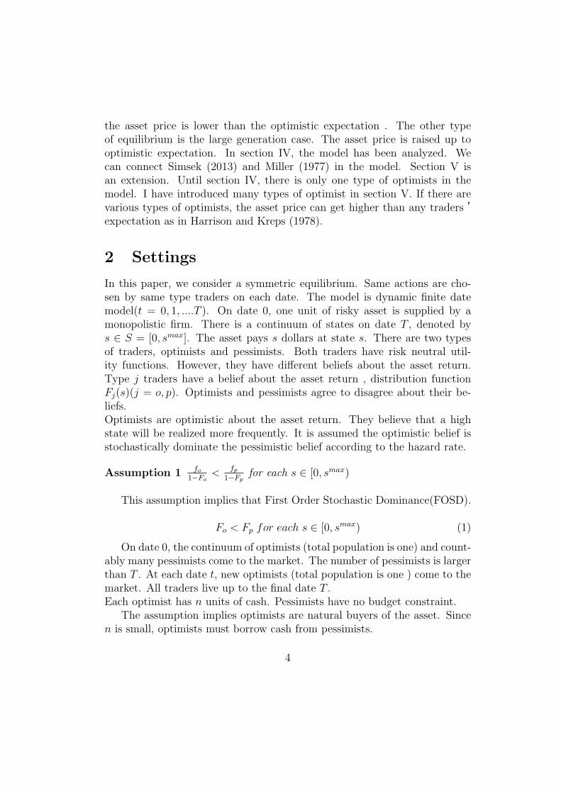
the asset price is lower than the optimistic expectation . The other typeof equilibrium is the large generation case. The asset price is raised up tooptimistic expectation. In section IV, the model has been analyzed. Wecan connect Simsek (2013) and Miller (1977) in the model. Section V isan extension. Until section IV, there is only one type of optimists in themodel. I have introduced many types of optimist in section V. If there arevarious types of optimists, the asset price can get higher than any traders ’expectation as in Harrison and Kreps (1978).

2 Settings

In this paper, we consider a symmetric equilibrium. Same actions are cho-sen by same type traders on each date. The model is dynamic finite datemodel(t = 0, 1, ....T ). On date 0, one unit of risky asset is supplied by amonopolistic firm. There is a continuum of states on date T , denoted bys ∈ S = [0, smax]. The asset pays s dollars at state s. There are two typesof traders, optimists and pessimists. Both traders have risk neutral util-ity functions. However, they have different beliefs about the asset return.Type j traders have a belief about the asset return , distribution functionFj(s)(j = o, p). Optimists and pessimists agree to disagree about their be-liefs.Optimists are optimistic about the asset return. They believe that a highstate will be realized more frequently. It is assumed the optimistic belief isstochastically dominate the pessimistic belief according to the hazard rate.

Assumption 1 fo1−Fo

< fp1−Fp

for each s ∈ [0, smax)

This assumption implies that First Order Stochastic Dominance(FOSD).

Fo < Fp for each s ∈ [0, smax) (1)

On date 0, the continuum of optimists (total population is one) and count-ably many pessimists come to the market. The number of pessimists is largerthan T . At each date t, new optimists (total population is one ) come to themarket. All traders live up to the final date T .Each optimist has n units of cash. Pessimists have no budget constraint.

The assumption implies optimists are natural buyers of the asset. Sincen is small, optimists must borrow cash from pessimists.

4

t = 0

t = 1

t = 2

t = T

PessimistsOptimists at each date

0 1 2

optimists trade on their birth date

Figure 1: Generation

Optimists who come to the market on date t have a chance to buy the assetor the security only on date t. Optimists buy the security or the asset, andthey wait until s is realized (date T ). This optimists settings is similar toover-lapping generation models, in which traders can participate in marketsonly in two date. In this model, the date t optimists and the date t+1 opti-mists is linked through pessimists. This assumption implies that pessimistsare professional traders (like managers in hedge funds) and optimists are not.Optimists have limited cash, an optimistic belief and little financial networkadvantages.Another interpretation of this settings is that professional traders can tradervery faster than optimists. Although the model is dynamic, the date T maymean one day or one hour later from the date 0. Only pessimists can use acomputer and can trade each “date” t. The equilibrium of this model is verysimple one and these securitization can be easily generated by hedge funds.Pessimists have a plenty of cash and have no budget constraints. They arenatural lenders of cash. Optimists don’t have enough cash for buying theasset. So, they must borrow some cash from pessimists. All borrowing con-tract in this economy is subject to a collateral constraint. Promises made byborrowers must be collateralized by assets or securities. These constraints arethe same as that of Simsek(2013) which is originally in Geanakoplos(2003,2010). In this paper, consider a simple debt contract. The borrowers promisedoes not depend on the state s on date T . These contract are very simple,

5

lend cash

sell contract

sell security

lend cash

sell contract

pessimist

pessimistoptimist j0

lend cash

sell asset

optimist j1

Firm

Figure 2: The sequence of the trade

but the equilibrium of the model can explain one struture of common col-lateralized loan model. Moreover, we can introduce the securitzation to themodel very easily.A collateraled loan contract on date 0 is defined as (γ0, ϕ0) for one unit of theasset collateral. ϕ0 is the amount of cash borrowing and γ0 is the borrowerspromise payment after the revealment of s(date T ). If the borrowers cannotpay γ0 on date T , they must give one unit of the asset as a collateral tothe lenders. The cash borrowers make a take-it-or-leave-it offer (γ0, ϕ0) tolenders.Since only one type of the asset exists on date 0, the loan contract must becollateralized by the asset.

• If the asset return s is high (s > γ0), the optimist can pay the promiseγ0 to the pessimist.

• If the asset return s is low (s ≤ γ0), the optimist gives the asset returns to the pessimist.

6

In other words, borrowers give min(s, γ0) to lenders in a loan contract(γ0, ϕ0).Then, the loan payoff ismin(s, γ0). Pessimists evaluate the payoff as Ep[min(s, γ)]and optimists evaluate it as Eo[min(s, γ0)]. The evaluation of optimists ishigher than the pessimists’ evaluation for the assumption of FOSD.

Eo[min(s, γ0)] > Ep[min(s, γ0)]

So, there is an incentive for trading the loan contract.The loan lender can securitize the loan contract and sell it to the other tradersat next date 1. He can issue loan backed securities whose payoff is min(s, γ0)with price q1. For the sake of simplicity, suppose only one pessimist lendscash to all optimist at each date. (Pessimists have no budget constraints.)This pessimist can issue the security with monopolistic power On next date.On date 1, traders can make loan contract with collateralized the security.A loan contract collateralized by the security is defined as (γ, ϕ) for one unitof the security. Consider a security which has a return min(s, γ′) on date T isused as collateral. ϕ is the amount of cash borrowing and γ is the borrowers’promise payment after the revealment of min(s, γ′), i.e., (γ′ > γ). If theborrowers cannot pay γ, they must give the securities as collateral to thelenders. The cash borrowers make a take-it-or-leave-it offer (γ, ϕ) to lenders.The security payoff is min(s, γ′). If s is low on date T , the loan default mayoccur. In this case, the borrowers must give the security to the lenders.

• If the security return is high (min(s, γ′) > γ), the optimist can pay thepromise γ to the pessimist.

• If the security return is low (min(s, γ′) ≤ γ), the optimist gives thesecurity return min(s, γ) to the pessimist.

That is, borrowers give min[min(s, γ′), γ] = min(s, γ) to lenders in a loancontract (γ, ϕ).On each date t ≥ 1, traders who lent cash at previous date t − 1 with loancontract (γ, ϕ) can issue loan backed securities which securitize loan contractsand the security payoff is min(s, γ). ϕ can be interpreted as a cost of issuingthe security for lenders.

7

pessimist

pessimistoptimist

optimist

pessimistoptimist

s

Firm

t = 0

t = 1

t = 2

min(s, γ0)

min(s, γ1)

min(s, γ0)

min(s, γ1)

min(s, γ2)

min(s, γ2)

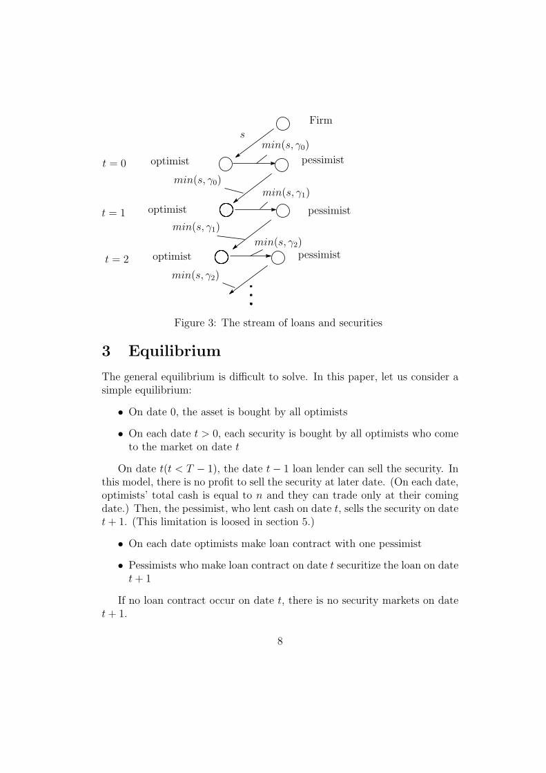
Figure 3: The stream of loans and securities

3 Equilibrium

The general equilibrium is difficult to solve. In this paper, let us consider asimple equilibrium:

• On date 0, the asset is bought by all optimists

• On each date t > 0, each security is bought by all optimists who cometo the market on date t

On date t(t < T − 1), the date t− 1 loan lender can sell the security. Inthis model, there is no profit to sell the security at later date. (On each date,optimists’ total cash is equal to n and they can trade only at their comingdate.) Then, the pessimist, who lent cash on date t, sells the security on datet+ 1. (This limitation is loosed in section 5.)

• On each date optimists make loan contract with one pessimist

• Pessimists who make loan contract on date t securitize the loan on datet+ 1

If no loan contract occur on date t, there is no security markets on datet+ 1.

8

3.1 Pessimists’ Loan Problem

Optimists make a take-it-or-leave-it offer (γt, ϕt) to the pessimist on date t ≤T −2. If the pessimist accept the offer, he lends ϕt cash and sells the securitywith price qt+1 on date t + 1. Then, pessimist accept the offer if ϕt ≤ qt+1.Since the security price qt+1 depends on the payment γt(the security returnis min(s, γt)), let qt+1(γt) be the price of the security collateralized by theloan payment γt.For pessimists, the loan contract is only way to earn cash. Since there aremany pessimists, their lending competition implies no-arbitrage condition:

ϕt = qt+1(γt) (2)

on date T − 1, the pessimist cannot sell the security at next date T . Theloan payoff is min(s, γT−1). Then, pessimist competition imply:

ϕT−1 = Ep[min(s, γT−1)] (3)

On date t+ 1, the date t lender can issue the security with monopolisticpower. Optimists have their own cash n and can borrow cash ϕt+1 per unitof the security from pessimists with loan contract. Then, let at+1 be thedemand of the security, the optimists’ budget constraint is:

at+1qt+1 ≤ n+ at+1ϕt+1 (4)

However, the security seller (and the date t lender) can choose the secuiryprice qt+1. The seller’s profit is at+1qt+1. So, he can raise the price untiloptimists’ budget constratin is equally satisfied. That is:

at+1qt+1 = n+ at+1ϕt+1 (5)

on date 0, monopolistic firm choose the asset price by the same manner.The date 0 optimists’ budget constraint is:

a0p = n+ a0ϕ0 (6)

a0 is optimists’ asset demand.

9

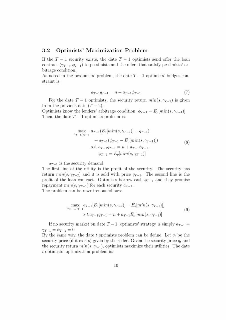
3.2 Optimists’ Maximization Problem

If the T − 1 security exists, the date T − 1 optimists send offer the loancontract (γT−1, ϕT−1) to pessimists and the offers that satisfy pessimists’ ar-bitrage condition.As noted in the pessimists’ problem, the date T − 1 optimists’ budget con-straint is:

aT−1qT−1 = n+ aT−1ϕT−1 (7)

For the date T − 1 optimists, the security return min(s, γT−2) is givenfrom the previous date (T − 2).Optimists know the lenders’ arbitrage condition, ϕT−1 = Ep[min(s, γT−1)].Then, the date T − 1 optimists problem is:

maxaT−1,γT−1

aT−1(Eo[min(s, γT−2)]− qT−1)

+ aT−1(ϕT−1 − Eo[min(s, γT−1)])

s.t. aT−1qT−1 = n+ aT−1ϕT−1,

ϕT−1 = Ep[min(s, γT−1)]

(8)

aT−1 is the security demand.The first line of the utility is the profit of the security. The security hasreturn min(s, γT−2) and it is sold with price qT−1. The second line is theprofit of the loan contract. Optimists borrow cash ϕT−1 and they promiserepayment min(s, γT−1) for each security aT−1.The problem can be rewritten as follows:

maxaT−1,γT−1

aT−1[Eo[min(s, γT−2)]− Eo[min(s, γT−1)]]

s.t.aT−1qT−1 = n+ aT−1Ep[min(s, γT−1)](9)

If no security market on date T − 1, optimists’ strategy is simply aT−1 =γT−1 = ϕT−1 = 0By the same way, the date t optimists problem can be define. Let qt be thesecurity price (if it exists) given by the seller. Given the security price qt andthe security return min(s, γt−1), optimists maximize their utilities. The datet optimists’ optimization problem is:

10

maxat,γt

at(Eo[min(s, γt−1)]− qt)

+ at(ϕt − Eo[min(s, γt)])

s.t. atqt = n+ atϕt,

ϕt = qt+1(γt)

(10)

at is the security demand. qt+1(γt) is the price function of the date t+ 1security. The date t + 1 security depends on the date t loan contract (γt).This function will be calculated by backward induction.If no security exists, at = γt = ϕt = 0on date 0, the asset is supplied by a monopolistic firm with price p. Similarly,the date 0 optimists’ problem:

maxa0,γ0

a0(Eo[s]− p)

+ a0(ϕ0 − Eo[min(s, γ0)])

s.t. a0p = n+ a0ϕ0,

ϕ0 = q1(γ0)

(11)

a0 is the asset demand. q1(γ0) is the price function of the date 1 security.The date 1 security depends on the date 0 loan contract (γ0).

3.3 Equilibrium Definition

Definition 1 An equilibrium consists of the asset price p, the each date secu-rity price {qt}t=1,2,..,T−1, loan contract {(γt, ϕt)}t=0,1,...,T−1, the asset demanda0 and the security demand {at}t=1,2,..,T−1. They satisfy the following condi-tions:

• Given γt−1 and qt, at and γt solves the date t optimists’ problem

• At each date t, the loan contract (γt, ϕt) satisfy the pessimists’ arbitragecondition

• Market clearing condition

11

a0 = 1 (asset market clearing on date 0)

at =

{1 if the date t security exists at t ≥ 1

0 otherwise

3.4 Small T Case

The equilibrium is solved by backward induction from T −1. The date T −1optimists are price takers. The security price qT−1 is given by the seller. Forthe date T − 1 optimists, the security return min(s, γT−2) is given by theprevious date (T − 2). Optimists know the arbitrage condition of pessimistsϕT−1 = Ep[min(s, γT−1)].Then, the date T − 1 optimists problem is:

maxaT−1,γT−1

aT−1[Eo[min(s, γT−2)]− Eo[min(s, γT−1)]]

s.t.aT−1qT−1 = n+ aT−1Ep[min(s, γT−1)](12)

By solving the problem, qT−1 and γT−1 are determined.

Lemma 1 Given γT−2, the equilibrium security price (qT−1 and the loancontract γT−1) is determinded by the following two equations:

qT−1 =

∫ γT−1

0

sdFp +1− Fp(γT−1)

1− Fo(γT )

∫ smax

γT−1

min(s, γT−1)dFo

qT−1 = n+ Ep[min(s, γT−1)]

Proof 1 In the equilibrium, all security is bought by optimists. Then, aT−1 >0. From the budget constraint:

aT−1 =n

qT−1 − Ep[min(s, γT−1)]

Substitute this by the objective function:

n/α

qT−1 − Ep[min(s, γT−1)][Eo[min(s, γT−2)]− Eo[min(s, γT−1)]] (13)

12

FOC imply:

1− Fo(γT−1)

qT−1 − Ep[min(s, γT−1)]+(1−Fp(γT−1))

Eo[min(s, γT−2)]− Eo[min(s, γT−1)]

(qT−1 − Ep[min(s, γT−1)])2= 0

Let q1T−1 be the security price that satisfies FOC:

q1T−1 =1− Fp(γT−1)

1− Fo(γT−1){Eo[min(s, γT−2)]−Eo[min(s, γT−1)]}+Ep[min(s, γT−1)]

By differentiating in γT−1:

dq1T−1

dγT−1

= (1− Fp(γT−1)

1− Fo(γT−1))′{Eo[min(s, γT−2)]− Eo[min(s, γT−1)]}

= (fp(γT−1)

1− Fo(γT−1)+

fo(γT−1)(1− Fp(γT−1))

(1− Fo(γT−1))2){Eo[min(s, γT−2)]− Eo[min(s, γT−1)]}

From the assumption 1 ( fo1−Fo

< fp1−Fp

), this q1T−1 is decreasing in γT−1.

Because 0 ≤ γT−1 ≤ γT−2, the range of q1T−1 is determined:

Ep[min(s, γT−2)] ≤ q1T−1 ≤ Eo[min(s, γT−2)]

In equilibrium, all securities are bought by optimists. The market clearingimplies aT−1 = 1. From the budget constraint:

qT−1 = n+ Ep[min(s, γT−1)]

Let q2T−1 be the price qT−1 satisfies this condition:

q2T−1 = n+ Ep[min(s, γT−1)]

Because 0 ≤ γT−1 ≤ γT−2, the range of q2T−1 is determined:

n ≤ q2T−1 ≤ n+ Ep[min(s, γT−2)]

q2T−1 is increasing in γT−1.Because both q1T−1 and q2T−1 are continuous, there is only one γT−1 which

satisfies two equations. (see Appendix)Given γT−2, γT−1 is uniquely determined .Then qT−1 is also uniquely determined.//

13

T − 2 T − 1T − 3

min(s, γT−3) qT−1(γT−2)

Pessimist

qT−2

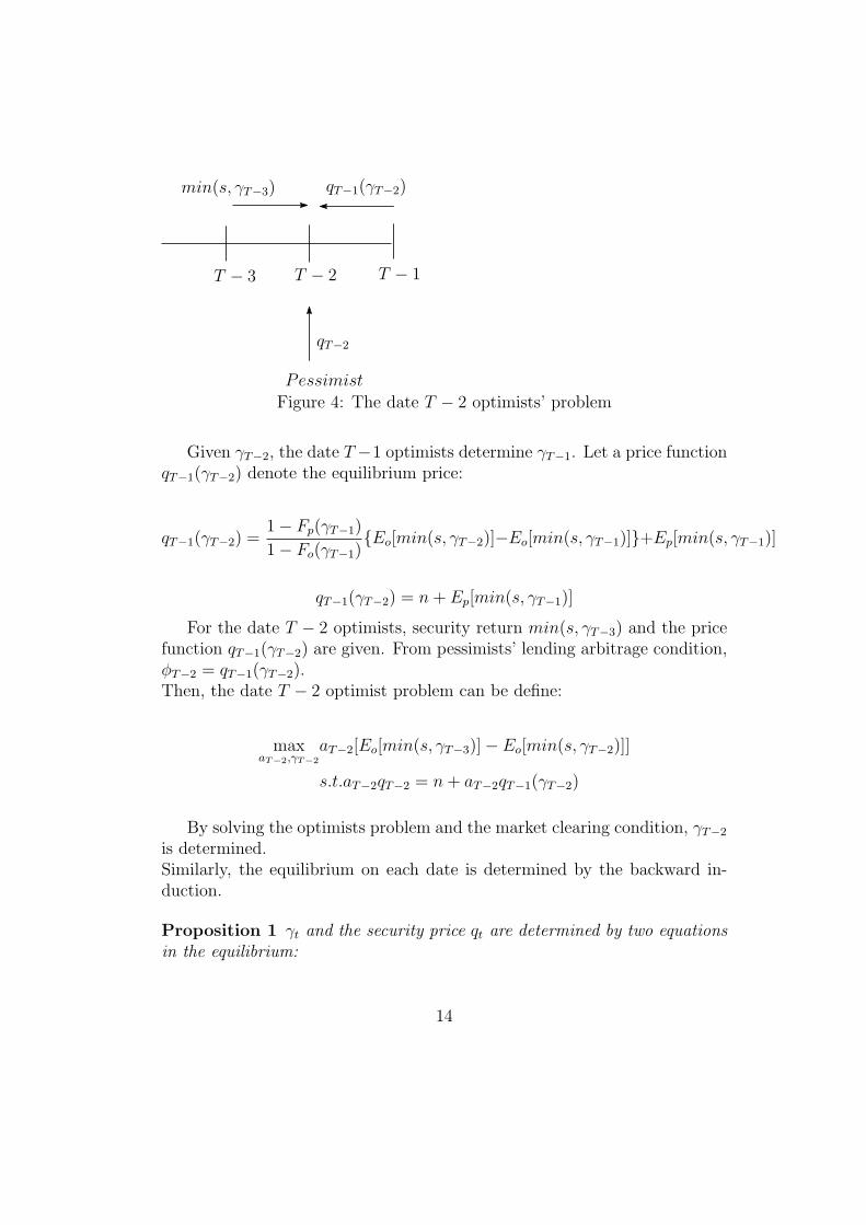
Figure 4: The date T − 2 optimists’ problem

Given γT−2, the date T−1 optimists determine γT−1. Let a price functionqT−1(γT−2) denote the equilibrium price:

qT−1(γT−2) =1− Fp(γT−1)

1− Fo(γT−1){Eo[min(s, γT−2)]−Eo[min(s, γT−1)]}+Ep[min(s, γT−1)]

qT−1(γT−2) = n+ Ep[min(s, γT−1)]

For the date T − 2 optimists, security return min(s, γT−3) and the pricefunction qT−1(γT−2) are given. From pessimists’ lending arbitrage condition,ϕT−2 = qT−1(γT−2).Then, the date T − 2 optimist problem can be define:

maxaT−2,γT−2

aT−2[Eo[min(s, γT−3)]− Eo[min(s, γT−2)]]

s.t.aT−2qT−2 = n+ aT−2qT−1(γT−2)

By solving the optimists problem and the market clearing condition, γT−2

is determined.Similarly, the equilibrium on each date is determined by the backward in-duction.

Proposition 1 γt and the security price qt are determined by two equationsin the equilibrium:

14

� qt =q′t+1(γt)

1− Fo(γt){Eo[min(s, γt−1)]− Eo[min(s, γt)]}

+ qt+1(γt)

� qt = n+ qt+1(γt)

Proof 2 The date T − 2 optimists’ problem:

maxaT−2,γT−2

aT−2[Eo[min(s, γT−3)]− Eo[min(s, γT−2)]]

s.t.aT−2qT−2 = n+ aT−2qT−1(γT−2)

By FOC imply:

qT−2 =q′T−1(γT−2)

1− Fo(γT−2){Eo[min(s, γT−3)]− Eo[min(s, γT−2)]}

+ qT−1(γT−2)

In the equilibrium, all securities are bought by optimists. The marketclearing implies aT−t = 1.From the budget constraint:

qT−2 = n+ qT−1(γT−2)

γT−2 is uniquely determined by these two equations. Given γT−3, qT−2

is uniquely determined. Let qT−2(γT−3) denote the equilibrium security pricegiven γT−3.

By using qT−2(γT−3), the date T − 3 optimists’ problem is written.

maxaT−3,γT−3

aT−3[Eo[min(s, γT−4)]− Eo[min(s, γT−3)]]

s.t.aT−3qT−3 = n+ aT−3qT−2(γT−3)

By continuing the backward induction, the date t problem is written byusing a security price function qt+1(γt).Given γt−1 and qt, the date t optimists problem:

15

maxat,γt

at(Eo[min(s, γt−1)]− Eo[min(s, γt)])

s.t. atqt = n+ atqt+1(γt)(14)

FOC and the market clearing imply:

� qt =q′t+1(γt)

1− Fo(γt){Eo[min(s, γt−1)]− Eo[min(s, γt)]}

+ qt+1(γt)

� qt = n+ qt+1(γt)

Appendix A.2 shows the equilibrium γt uniquely exists.//

Similarly, the asset price p is written by using q1(γ0). The date 0 optimistsproblem is written by using q1(γ0).

maxa0,γ0

a0{Eo[s]− Eo[min(s, γ0)]}

s.t.a0p = n+ a0q1(γ0)

Proposition 2 γ0 and the asset price p are determined by these two equa-tions in the equilibrium:

� p =q′1(γ0)

1− Fo(γ0){Eo[s]− Eo[min(s, γ0)]}+ q1(γ0)

� p = n+ q1(γ0)

Proof 3 By FOC of the date 0 problem:

1− Fo(γ0)

p− q1(γ0)+ q′1(γ0)

Eo[s]− Eo[min(s, γ0)]

p− q1(γ0)= 0

FOC imply:

� p =q′1(γ0)

1− Fo(γ0){Eo[s]− Eo[min(s, γ0)]}+ q1(γ0)

16

In equilibrium, a0 = 1 by the market clearing.

p = n+ q1(γ0) (15)

//

From the asset price and the security price:

p = n+ q1(γ0)

= 2n+ q2(γ2) = ...

= Tn+ Ep[min(s, γT−1)]

(16)

Optimists’ total cash Tn raise the asset price. In this market, the highestasset price is optimistic expectation of asset return Eo[s]. At next subsection,this price is achieved in the large generation case.

3.5 Large T Case

If T is large enough, at some date t′, the security is bought by the optimistsown cash n. on date t′, the security payoff is min(s, γt′−1). Since the sellerof the security have monopolistic power, the security price is equal to theoptimistic expectation:

qt′ = Eo[min(s, γt′−1)] (17)

After date t′, there is no security market. (qt = 0 for t > t′)Given γt′−2 , the date t′ − 1 optimist problem is:

maxat′−1,γt′−1

at′−1{Eo[min(s, γt′−2)]− Eo[min(s, γt′−1)]}

s.t. at′−1qt′−1 = n+ at′−1Eo[min(s, γt′−1)](18)

By solving the problem, the security price qt′−1 is:

qt′−1 =

∫ γt′−1

0

sdFo +1− Fo(γt′−1)

1− Fo(γt′−1)

∫ smax

γt′−1

min(s, γt′−2)dFo

= Eo[min(s, γt′−2)]

17

This equation and qt′−1 = n+Eo[min(s, γt′−1)](From at′−1 = 1) determineγt′−1.By the backward induction, the date t security price is calculated.

proposition 1 If T is large enough, the security price at each date t givenγt−1 is:

qt = Eo[min(s, γt−1)]

The asset price is:

p = Eo[s]

Proof 4 Assume the security price function qt+1(γt) = Eo[min(s, γt)]Given γt−1 and qt, the date t optimist problem is:

maxat,γt

at{Eo[min(s, γt−1)]− Eo[min(s, γt)]}

s.t. atqt = n+ atEo[min(s, γt)](19)

This is almost same form as the date t′ − 1 problem.FOC implies the security price qt is Eo[min(s, γt−1)].Since the security price on date t′ is qt′ = Eo[min(s, γt′−1)], the securityprice qt is Eo[min(s, γt−1)] by the backward induction. γt is determined bythe market clearing condition at = 1:

Eo[min(s, γt−1)] = n+ Eo[min(s, γt)]

The date 0 problem is:

maxa0,γ0

a0{Eo[s]− Eo[min(s, γ0)]}

s.t. a0p = n+ a0Eo[min(s, γ0)](20)

This is also the same form on date t′ − 1. FOC implies that the assetprice is:

p = Eo[min(s, smax)] = Eo[s] (21)

γ0 is determined by the market clearing condition at = 1:

18

0 s

Return

γt′−1

γt′−1

γ1

γ1

γ0

γ0

smax

smax

Date 1

Date t′

Date 0Optimist

Optimist

Optimist

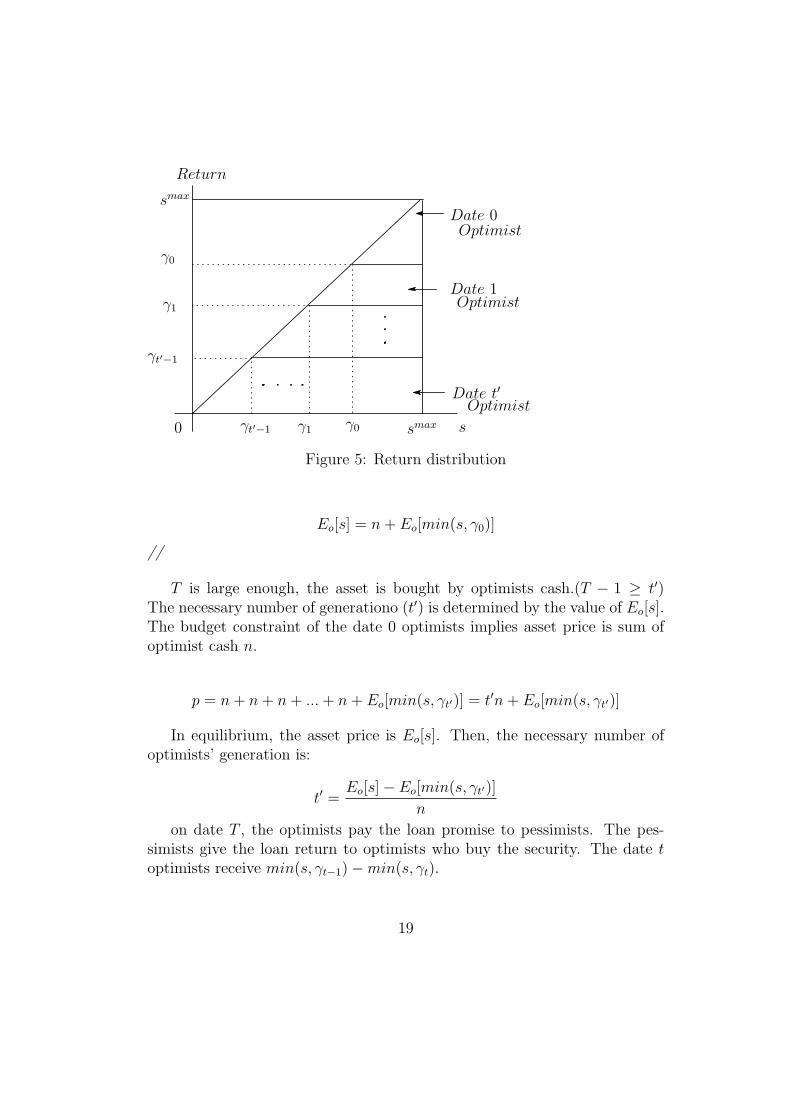
Figure 5: Return distribution

Eo[s] = n+ Eo[min(s, γ0)]

//

T is large enough, the asset is bought by optimists cash.(T − 1 ≥ t′)The necessary number of generationo (t′) is determined by the value of Eo[s].The budget constraint of the date 0 optimists implies asset price is sum ofoptimist cash n.

p = n+ n+ n+ ...+ n+ Eo[min(s, γt′)] = t′n+ Eo[min(s, γt′)]

In equilibrium, the asset price is Eo[s]. Then, the necessary number ofoptimists’ generation is:

t′ =Eo[s]− Eo[min(s, γt′)]

n

on date T , the optimists pay the loan promise to pessimists. The pes-simists give the loan return to optimists who buy the security. The date toptimists receive min(s, γt−1)−min(s, γt).

19

4 Analysis

4.1 The Structure of The Asset Price

The equilibrium security price is determined by two equations:

� qt =q′t+1(γt)

1− Fo(γt){Eo[min(s, γt−1)]− Eo[min(s, γt)]}

+ qt+1(γt)

� qt = n+ qt+1(γt)

The equilibrium asset price is also determined by two equations:

� p =q′1(γ0)

1− Fo(γ0){Eo[s]− Eo[min(s, γ0)]}

+ q1(γ0)

� p = n+ q1(γ0)

These price equations imply:

n =q′t+1(γt)

1− Fo(γt){Eo[min(s, γt−1)]− Eo[min(s, γt)]} (22)

n =q′1(γ0)

1− Fo(γ0){Eo[s]− Eo[min(s, γ0)]} (23)

n is the optimists’ cash on each date.On date t, optimists use their cash to receive the divided return:

Eo[min(s, γt−1)]− Eo[min(s, γt)] (24)

On date 0:

Eo[s]− Eo[min(s, γ0)] (25)

The optimists buy the right to receive one part of the asset return. Theasset price structures show the return distribution.Each return division can be interpreted as one of the tranche.

20

Loan Lending

Optimist cash n

Buy Asset

Pessimist

F irm

Figure 6: Cash flow in one generation case

The early optimists (like t = 0) is very risky because the optimists can getpositive payoff only in the high return state, like a “junior” tranche. Simi-larly, the middle return state is like “mezzanine” tranche and the lower returnstate is like “senior” tranche.By a collateral loan contract and a simple securitization, the complex financ-ing technologies can be constructed in the model.

4.2 The Linkage: From Simsek to Miller

If the securitization is not allowed, the asset price is equal that given bySimsek(2013), which is equal to that of the T = 1 model.

Only one generation of the traders participate in the market. Optimists’loan borrowing is ϕ0 = Ep[min(s, γ0)]. Their budgets are n+ Ep[min(s, γ0)]In T = 1 case, the equilibrium asset price is deduced by two equations.

p =

∫ γ0

0

sdFp +1− Fp(γ0)

1− Fo(γ0)

∫ smax

γ0

sdFo

and

p = n+ Ep[min(s, γ0)]

These two equations are exactly the same as that of Simsek(2013).In his model, the asset price is heavily affected by the collateral economy.If high return states occur, optimists repay the loan and still have the asset.If low return states occur, optimists must give the asset to the pessimists as

21

collateral.The first equation pictures this situation. High return states (s > γ0) areevaluated by optimistic belief(Fo) and low return states(s < γ0) are evaluatedby pessimistic belief(Fp).In T = 1 case, the economy is the same as Simsek(2013). However, if T getslarger, the economy go to the model of the heterogeneous belief bubbles, likeMiller(1977).In T = 2 case, the securitization is allowed. Optimists loan borrowing on date0 is ϕ0 = q1(γ0). Their budget is n+q1(γ0). Because q1(γ0) > Ep[min(s, γ0)],optimists can use bigger budget. As a result, the asset gets higher.In T = 2 case, the equilibrium asset price:

p = n+ q1(γ0) = 2n+ Ep[min(s, γ1)]

The high price is sustained by new optimists’ cash.Assume pessimists’ evaluation about the asset return is 0 (Fp(0) = 1). Inthis case, pessimists evaluation about the loan lending Ep[min(s, γ)] = 0 forany γ. So, the T = 2 security price on date 1 is equal to q1(γ0) = n. Theasset price of T − 2 case is equal to n+ q1(γ0) = 2n.In two generation case, the date 0 optimists can use cash from the date 1optimists. The existence of the date 1 optimists raise the asset price.By making loan contracts, pessimists can sell securities on next date. Thepessimist has a speculative incentive for the loan contract.

By the same logic, the asset price gets higher if T gets larger. Large Timplies that many optimists come to the market. Their total cash raise theasset price.

From small T case, the asset price:

p = Tn+ Ep[min(s, γT−1)]

If T is large enough, the asset price is equal to Eo[s].In Miller(1977), the asset price is equal to the optimistic expectation. Inmy model, Miller price is achieved by the coordination through a financialtechnology, securitization.Optimists have incentive to buy the asset, but they does not have enoughcash. Without the security market, they have no way to cooperate with eachother. The security and the loan contract play a role in enabling their coop-eration.The loan contract causes the security, which in turn causes the loan contract.

22

Loan Lending

Optimist

asset

Pessimist

security

Optimist

F irm

Buy

Buy

Figure 7: Cash flow in two generation case

The scheme allows each optimist to participate in the market.In Simsek(2013), optimists does not have enough cash, he must borrow cashfrom pessimist. Since the loan contract is limited, he must collateralize the as-set themselves. The asset price must be influenced by pessimistic belief(Fp).If T is large enough, pessimistic belief vanishes in the asset price. However,if there are no pessimists, the date 0 optimist have no way to bring enoughcash to buy the asset.The pessimists know that the new optimists will come to the market. So,they have strong incentive to lend their cash to the optimists. Lending cashis speculative action for the pessimist. They can sell the risk of the default ofoptimists to the other optimists by securitization. This is one of risk-shiftingproblem.(Shleifer and Vishny(1992))As a result, the asset return is shared by the optimists and the asset pricerises. This securities raise the utilities for both optimists and pessimists. Thesecurity technology compensate for incomplete financial market.If there are heterogeneous beliefs exists, completeness of security marketmake economy riskier. The advanced security market allow heterogeneousinvestor to act freely.

23

pessimist

pessimistoptimist

optimist

pessimistoptimist

Asset

Firm

t = 0

t = 1

t = 2

Security

Security

Loan

Loan

Loan

Security

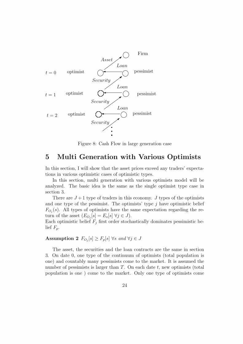
Figure 8: Cash Flow in large generation case

5 Multi Generation with Various Optimists

In this section, I will show that the asset prices exceed any traders’ expecta-tions in various optimistic cases of optimistic types.

In this section, multi generation with various optimists model will beanalyzed. The basic idea is the same as the single optimist type case insection 3.

There are J +1 type of traders in this economy. J types of the optimistsand one type of the pessimist. The optimists’ type j have optimistic beliefFOj

(s). All types of optimists have the same expectation regarding the re-turn of the asset (EOj

[s] = Eo[s] ∀j ∈ J).Each optimistic belief Fj first order stochastically dominates pessimistic be-lief Fp.

Assumption 2 FOj[s] ≥ Fp[s] ∀s and ∀j ∈ J

The asset, the securities and the loan contracts are the same in section3. On date 0, one type of the continuum of optimists (total population isone) and countably many pessimists come to the market. It is assumed thenumber of pessimists is larger than T . On each date t, new optimists (totalpopulation is one ) come to the market. Only one type of optimists come

24

on each date t. Let the date t optimists’ type be jt. Assume the order of{jt}t−0,1,2,..T−1 is exogenously given. All traders live up to the final date T .All optimists are initially endowed with small amount of cash n > 0 dollarsand zero unit of the asset. Pessimists have no budget constraint.Optimists who come to the market have a chance to buy the asset or thesecurity only on date t. They buy the asset or the security, and wait until sis realized (date T ).Pessimists have a plenty of cash and they have no budget constraints. Theyare natural lenders of cash.These settings are almost the same as single optimist models. However, theexistence of various optimists change the security sellers’ strategy. The datet seller can get higher return by selling the securities to high type optimistsafter date t. Then, there is an incentive for the seller to hold the securityand to postpone the trade.I have focused on the highest asset price equilibriium. If T is large enoughand all types j comes frequently, all sellers can trade with the highest typeof optimist.The focused equilibrium is, the same as the single type case, the single lenderand the monopolistic seller on each date. Note pt be the asset price whenthe trade occur on date t.

argmaxt pt = t0

The asset holder sells it on t0. On date t0, traders make loan contract.The lender (a pessimist) can sell the security after t0.Note qt1 be the security price when the trade occur on date t.

argmaxt>t0 qt1 = t1

By continuing this method, we get the stream tτ (τ = 0, 1, 2..). By using τinstead of t, the asset price is calculated like the single type optimists model.

Let p∗ and q∗τ be the highest price.

p∗ = pt0

q∗τ = qtττ

Let j∗τ be the type of optimists on date tτ .

j∗τ = jtτ

25

1 20t= 4 53

10 2τ =

6

Figure 9: Convert t to τ

On date tτ , the optimist buys the security with the loan contract. In thissection, for simplicity, T is assumed to be large enough. Some optimist canbuy the security at t′s by his own cash.For analyzing the asset price or the security price, the type jtτ problemon each tτ is solved. From each generation τ , ϕtτ is solved by pessimists’arbitrage condition.

ϕtτ = q∗τ+1

q∗τ ′ is solved by pessimists’ arbitrage condition.

q∗τ ′ = EOj∗τ ′[min(s, γτ ′−1)]

So, optimist type j∗0 problem at generation 0:

maxa0,γ0

a0{EOj∗0[s]− EOj∗0

[min(s, γ0)]}

s.t.a0p = n+ a0q∗1(γ0)

The budget constraint is satisfied by monopolistic power of the securityseller. Because type j∗0 is the highest optimists’ type, they evaluate EOj∗0

[s]−EOj∗0

[min(s, γ0)] higher than any other types.

The type j∗τ optimist problem at generation tτ :

maxaτ ,γτ

aτ{EOj∗τ[min(s, γτ−1)]− EOj∗τ

[min(s, γτ )]}

s.t.aτq∗τ = n+ aτq

∗τ+1(γτ )

26

Sell Security

pessimist

pessimistoptimist j∗0

Sell Asset

optimist j∗1

Firm

Loan Contract

Loan Contract

Sell Security

Figure 10: The stream of trade with various optimists

At generation τ ′, the security price is simply qτ ′ = EOj∗τ ′[min(s, γτ ′−1)].

j∗t′ is the type with the highest security price in equilibrium.By solving the problem on each trading date τ , p∗ and q∗τ are calculated.

Definition 2 Given trading date τ = 0, 1, 2, , ..τ ′, an equilibrium of varioustypes of optimists model consists of the asset price p∗, the each date securityprice {q∗τ}τ=1,2,..,τ ′, loan contract {(γτ , ϕτ )}τ=0,1,...,τ ′, the asset demand a0 andthe security demand {aτ}τ=1,2,..,T−1. They satisfy the following conditions:

• Given γτ−1 and q∗τ , aτ and γτ solves type j∗τ optimists’ problem on dateτ

• At each date τ , the loan contract (γτ , ϕτ ) satisfy pessimists arbitragecondition

• market clearing condition aτ = 1 for all τ

In the single optimist case, the asset price is equal to the optimistic ex-pected return: Eo[s]. In this model, the asset price is solved by the backward

27

induction like the single optimist model. However, in each generation, thedifferent types of the optimists buy the asset and the security. In this case,the asset price exceeds any trader’s expectation of the asset return.

proposition 2 In multi-generation model with the various types of the op-timists, the asset price exceeds optimistic traders’ expectation of the assetreturn:

p∗ ≥ Eo[s]

Proof 5 As noted above, the security price on date tτ ′ is Eoj∗τ ′[min(s, γτ ′−1)].

Since j∗τ ′ is the highest type of optimists, the security price qτ ′ = Eoj∗τ ′[min(s, γτ ′−1)]

is higher than the other types’ expected return of the security.

q∗τ ′ = Eoj∗τ ′[min(s, γτ ′−1)] ≥ EOj

[min(s, γτ ′−1)] ∀j

The optimist type j∗τ ′−1 buys the date tτ ′−1 security. The optimist problemon date tτ ′−1 is:

maxaτ ′−1,γτ ′−1

aτ ′−1{EOj∗τ ′−1

[min(s, γτ ′−2)]− Eoj∗τ ′−1

[min(s, γτ ′−1)]}

s.t.aτ ′−1q∗τ ′−1 = n+ aτ ′−1Eoj∗

τ ′[min(s, ¯γτ ′−1)]

By solving this problem,

q∗τ ′−1 =

∫ γτ ′−1

0

sdFOj∗τ ′+(1−FOj∗

t′(γτ ′−1))

∫ smax

γτ ′−1

min(s, γτ ′−2)dFOj∗

τ ′−1

1− FOj∗τ ′−1

(γτ ′−1)

The security demand is 1 in the equilibrium:

q∗τ ′−1 = n+ Eoj∗τ ′[min(s, γτ ′−1)]

The equilibrium is determined by these two equations. (See appendix A.3for the existence and uniqueness).If j∗τ ′−1 = j∗τ ′, i.e., the same type optimists buy the securities on both dates,the date τ ′ − 1 security price is simply EOj∗

τ ′−1

[min(s, γτ ′−1)] ( it is the same

as the single optimist model in large T case). In the various optimists model,

28

the optimist type who buys the security can be different on each date. Asnoted above, the security is bought by the optimists who can pay the highestsecurity price. Then, the security price is higher than the single optimistmodel.

q∗τ ′−1 ≥ EOj[min(s, γτ ′−2)] ∀j

The same calculation imply the security price exceeds the single optimisttype model on each date. If pessimists sell the security to the type j optimists,the security price on date tτ is equal to EOj

[min(s, γτ )]. However, the securityseller can choose the highest type optimists. So, the security price is higherthan any types of optimists’ expected return.

q∗τ ≥ Eoj [min(s, γτ−1)] ∀j ∀τBy the same logic, the asset price is higher than the single type optimist

model.

p∗ ≥ Eo[s] = Eoj [s] ∀j//

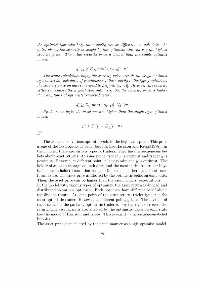
The existence of various optimist leads to the high asset price. This priceis one of the heterogeneous-belief bubbles like Harrison and Kreps(1978). Intheir model, there are various types of traders. They have heterogeneous be-liefs about asset returns. At some point, trader x is optimist and trader y ispessimist. However, at different point, x is pessimist and y is optimist. Theholder of an asset changes on each date, and the most optimistic trader buysit. The asset holder knows that he can sell it to some other optimist at somefuture state. The asset price is affected by the optimistic belief on each state.Then, the asset price can be higher than the asset holders’ expectations.In the model with various types of optimists, the asset return is divided anddistributed to various optimists. Each optimists have different belief aboutthe divided return. At some point of the asset return, trader type x is themost optimistic trader. However, at different point, y is so. The division ofthe asset allow the partially optimistic trader to buy the right to receive thereturn. The asset price is also affected by the optimistic belief on each statelike the model of Harrison and Kreps. This is exactly a heterogeneous-beliefbubbles.The asset price is calculated by the same manner as single optimist model.

29

0 s

Return

γτ ′−1

γτ ′−1

γ1

γ1

γ0

γ0

smax

smax

Oj∗0

Oj∗1

Oj∗τ ′

Figure 11: Return distribution with various optimists

In the single type case, each securities are bought by single optimist. Sincea single type optimist evaluate the security return, the asset price is equalto the optimistic expected return. On the other hand, each return area areevaluated by the highest type optimist in various types case. As a result, theasset price exceeds the optimistic expectation.The optimistic expectation about asset return is same:Eo[s]. The securitiza-tion technology divides the asset return and each optimist evaluate the eachpartition.

In Simsek(2013), asset return is evaluated by the optimist and the pes-simist. In equilibrium, as noted section IV, the asset price:

p =

∫ γ0

0

sdFp +1− Fp(γ0)

1− Fo(γ0)

∫ smax

γ0

min(s, γ0)dFo

This price equation imply that the optimist evaluate upper return area,and the pessimist evaluate lower area. Only high state part of optimisticbelief is used for determining the asset price in Simsek(2013). This is thereason why asset price is lower than Miller(1977).In this model, the most optimistic trader evaluates each area. Only hisoptimistic part of belief is used for evaluation of asset return. Since the

30

asset is priced by different beliefs, it is much more optimistic than anyone’sexpectation.

6 Conclusions

In this paper, by introducing the securitization and the simple dynamic set-ting to a collateral model, heterogeneous belief bubbles rises.In general, financial technologies, like securitizations, improve market effi-ciency. However, in heterogeneous belief model, securitizations allow manyoptimists to participate in markets and asset prices will be raised.Financial frictions can make the asset price lower. Many studies have re-ported that optimists have a heavy influence on pricing. Financial frictionslike borrowing constraints can prevent these traders to participate in mar-ket. In these situations, financial technologies loose this friction, and theasset price is raised by optimistic traders who have little cash.By the dynamic securitization scheme, the asset return is distributed to manypartitions. Each partition is very small, but this smallness allow various op-timist to receive payoff. Most optimistic traders evaluate their partitions andthe total asset price is equal to (or higher than) optimistic expected returnof asset in the case of single type of optimists (in the case of various types ofoptimists). Heterogeneous-belief bubbles occur.Before the asset return is realized, there are little incentive to correct theirbeliefs. If there are heterogeneity in markets, financial technologies can am-plify it.Financial technologies, like loan securitizations, improve market efficiency.They make the budget constrained traders to participate in the trade. Simul-taneously, they may make market instability through traders’ heterogeneity.

31

References

[1] Brunnermeier, M. ”Deciphering the Liquidity and Credit Crunch 2007-2008,” Journal of Economic Perspectives, 23(1), pp. 77-100. 2009.

[2] Brunnermeier, Markus K. and Martin Oehmke. ”The Maturity RatRace”, Journal of Finance 68(2), 483-521.

[3] Brunnermeier, M. K., and L. H. Pedersen (2009).“Market Liquidityand Funding Liquidity,”Review of Financial Studies, 22(6), 22012238.

[4] DeLong J. B., A. Shleifer, L. H.Summers and R. J. Waldmann(1990)”Noise Tradr Risk in Financial Markets” Jouranal of Political Economy,98(4)703-738.

[5] Fostel, A., and Geanakoplos, J. ”Tranching, CDS, and assetprices: How financial innovation can cause bubbles and crashes,”AEJ:Macroeconomics, 4(1)190-225. 2012.

[6] Genakoplos, J. ”The Leverage Cycle” in NBER Macroeconomics Annual2009, vol. 24 University of Chicago Press. 2010.

[7] Gorton, G., and Metrick, A (2011): ”Securitized banking and the runon repo,” Journal of Financial Economics, 104(3), 425-451.

[8] Gromb, D. and D. Vayanos . ”Equilibrium and Welfare in Markets withFinancially Constrained Arbitrageurs,” Journal of Financial Economics,(66)361-407. 2002.

[9] Harrison.J.M., and D. Kreps. ”Speculative Investor Behavior in a StockMarket with Heterogeneous Expectations” Quarterly Journal of Eco-nomics, (89) 323-326 1978.

[10] Kiyotaki, N. and J. Moore (1997), ”Credit Cycles,” Journal of PoliticalEconomy,Vol.105 (2), p.211-248.

[11] Krishnamurthy, A., S. Nagel, and D. Orlov (2011): ”Sizing Up Repo,”Working Paper, Stanford University.

[12] Miller, E. M.. ”Risk, Uncertainty, and Divergence of Opinion,” Journalof finance, 32(4), 1151-1168. 1977.

32

[13] Shleifer, A. and R. Vishny (1992), ”Liquidation Values and Debt Capac-ity: A Market Equilibrium Approach,”Journal of Finance, 47, p.1343-1366.

[14] Shleifer, A. and R. Vishny(1997), ”The Limits of Arbitrage”,Journal ofFinance, 52, p.35-55.

[15] Simsek, A.. ”Belief Disagreements and Collateral Constraints” Econo-metrica, 81(1), 1-53.2013.

7 Mathematical Appendix

7.1 Uniqueness of γT−1

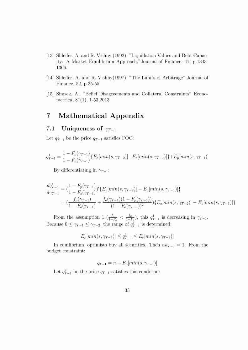
Let q1T−1 be the price qT−1 satisfies FOC:

q1T−1 =1− Fp(γT−1)

1− Fo(γT−1){Eo[min(s, γT−2)]−Eo[min(s, γT−1)]}+Ep[min(s, γT−1)]

By differentiating in γT−1:

dq1T−1

dγT−1

= (1− Fp(γT−1)

1− Fo(γT−1))′{Eo[min(s, γT−2)]− Eo[min(s, γT−1)]}

= (fp(γT−1)

1− Fo(γT−1)+

fo(γT−1)(1− Fp(γT−1))

(1− Fo(γT−1))2){Eo[min(s, γT−2)]− Eo[min(s, γT−1)]}

From the assumption 1 ( fo1−Fo

< fp1−Fp

), this q1T−1 is decreasing in γT−1.

Because 0 ≤ γT−1 ≤ γT−2, the range of q1T−1 is determined:

Ep[min(s, γT−2)] ≤ q1T−1 ≤ Eo[min(s, γT−2)]

In equilibrium, optimists buy all securities. Then αaT−1 = 1. From thebudget constraint:

qT−1 = n+ Ep[min(s, γT−1)]

Let q2T−1 be the price qT−1 satisfies this condition:

33

q2T−1 = n+ Ep[min(s, γT−1)]

Because 0 ≤ γT−1 ≤ γT−2, the range of q2T−1 is determined:

n ≤ q2T−1 ≤ n+ Ep[min(s, γT−2)]

q2T−1 is increasing in γT−1.Because both q1T−1 and q2T−1 are continuous, there is only one γT−1 which

satisfies two equations.Given γT−2, γT−1 is uniquely determined

7.2 Uniqueness of γt in Small T Case

I will show the existence of γT−2. γt can be shown by the similar way.

We must show for some γT−2 (0 ≤ γT−2 ≤ γT−3)satisfies the followingequation.

n =q′T−1(γT−2)

1− Fo(γT−2){Eo[min(s, γT−3)]− Eo[min(s, γT−2)]}

Let RHS be G(γT−2). The range of γT−2 is [0, γT−3].

G(γT−3) = 0 < n

G(0) = q′T−1(0)Eo[min(s, γT−3)]

If G(0) > n, at least one γT−2 satisfies the equation n = G(γT−2).qT−1(γT−2) must lie between optimistic expected return Eo[min(s, γT−2)]

and pessimistic expected return Ep[min(s, γT−2)].

Eo[min(s, γT−2)] ≥ qT−1(γT−2) ≥ Ep[min(s, γT−2)]

At γT−2 = 0, the optimistic and pessimistic evaluation of returnmin(s, γT−2)is 0.

qT−1(0) = Eo[min(s, 0)] = Ep[min(s, 0)] = 0

By differentiating at γT−2, 　 qT−1(γT−2) 　 must satisfy the followingequation

34

1− Fo(0) = 1 ≥ q′T−1(γT−2) ≥ 1 = 1− Fp(0)

This implies q′T−1(0) = 1.

G(0) = q′T−1(0)Eo[min(s, γT−3)] = Eo[min(s, γT−3)] > n

Then, G(0) is larger than n.(If Eo[min(s, γT−3)] < n, the date T − 2 optimists can buy the security bytheir own cash. (Large n case)) At least one γT−2 satisfies n = G(γT−2).There may be many γT−2 satisfies the equation. As the security seller cansell the security at the highest price, he can choose the equilibrium γT−2 thatbring the highest price qT−2.

γT−2 =argmaxγ n+ qT−1(γ)

s.t.n = G(γ)

Then, γT−2 is uniquely determined. Similarly, γt is uniquely determinedon each date.

7.3 Uniqueness of γτ in Various Types of Optimists

The proof is almost same as that in single type case. I will show the existenceof γτ ′−2. γτ can be shown by the similar way.

I must show for some γτ ′−2 (0 ≤ γτ ′−2 ≤ γτ ′−3)satisfies the followingequation.

n =q∗

′

τ ′−1(γτ ′−2)

1− Foj∗τ ′−2

(γτ ′−2){Eoj∗

τ ′−2

[min(s, γτ ′−3)]− Eoj∗τ ′−2

[min(s, γτ ′−2)]}

Let RHS be G(γτ ′−2). The range of γτ ′−2 is [0, γτ ′−3].

G(γτ ′−3) = 0 < n

G(0) = q∗′

τ ′−1(0)Eoj∗τ ′−2

[min(s, γτ ′−3)]

If G(0) > n, at least one γτ ′−2 satisfies the equation n = G(γτ ′−2).Since T is large enough, in multi types of optimists case, q∗t′−1(γτ ′−2) must

35

be larger than Eoj∗τ ′−2

[min(s, γτ ′−2)]. (If not so, the seller of the security can

raise the security price.)

q∗τ ′−1(γτ ′−2) ≥ Eoj∗τ ′−2

[min(s, γτ ′−2)]

At γτ ′−2 = 0, the optimistic evaluation of return min(s, γτ ′−2) is 0.

q∗τ ′−1(0) = Eoj∗τ ′−2

[min(s, 0)] = 0

By differentiating at γτ ′−2,　 qt′−1(γτ ′−2)　 must satisfy the followingequation

q∗′

τ ′−1(γτ ′−2) ≥ 1 = 1− Foj∗τ ′−2

(0)

This implies q∗′

τ ′−1(0) ≥ 1.

G(0) = q∗′

τ ′−1(0)Eoj∗τ ′−2

[min(s, γτ ′−3)] ≥ Eoj∗τ ′−2

[min(s, γτ ′−3)] > n

Then, G(0) is larger than n, and At least one γτ ′−2 satisfies n = G(γτ ′−2).There may be many γτ ′−2 satisfies the equation. As the security seller cansell the security at the highest price, he can choose the equilibrium γτ ′−2 thatbring the highest price q∗τ ′−2.

γτ ′−2 =argmaxγ n+ q∗τ ′−1(γ)

s.t.n = G(γ)

Then, γτ ′−2 is uniquely determined. Similarly, γτ is uniquely determinedon each date.

36