Sectoral Heterogeneity in the Employment Effects of Job

Creation Schemes in Germany∗

Marco Caliendo†, Reinhard Hujer‡ and Stephan L. Thomsen§

∗DIW, Berlin and IZA, Bonn†J.W.Goethe-University, Frankfurt/Main, IZA, Bonn, ZEW, Mannheim‡J.W.Goethe-University, Frankfurt/Main

Revised version: October 26, 2005

Abstract

Job creation schemes (JCS) have been one important programme of active labour market policy in Germany aiming at

the re-integration of hard-to-place unemployed individuals into regular employment. In contrast to earlier evaluation

studies of these programmes based on survey data, we use administrative data containing more than 11,000 participants

for our analysis and hence, can take effect heterogeneity explicitly into account. We focus on effect heterogeneity caused

by differences in the implementation of programmes (economic sector, types of support and implementing institutions).

The results are rather discouraging and show that in general, JCS are unable to improve the re-integration chances of

participants into regular employment.

Keywords: Evaluation – Job Creation Schemes - Employment Effects – Sectoral Heterogeneity

JEL Classification: H43, J68, C13

∗The authors thank two anonymous referees for valuable comments which helped to improve the paper. Financial support of

the Institute for Employment Research (IAB) within the project ‘Effects of Job Creation and Structural Adjustment Schemes’ is

gratefully acknowledged. The usual disclaimer applies. A supplementary appendix to this paper is available on request from the

authors and can also be downloaded under http:/www.wiwi.uni-frankfurt.de/professoren/hujer/papers/sectoralancappendix.pdf. A

previous version of this paper circulated as ‘Individual Employment Effects of Job Creation Schemes in Germany with Respect to

Sectoral Heterogeneity’.

Corresponding author: Marco Caliendo, DIW Berlin, Dep. of Public Economics, Konigin-Luise-Str. 5, 14195 Berlin, phone: +49-30-

89789-154, fax: +49-30-89789-9154.†Marco Caliendo is Senior Research Associate at the German Institute for Economic Research (DIW) in Berlin and Research

Fellow of the IZA, Bonn, e-mail: mcaliendo@diw.de.‡Reinhard Hujer is Professor of Statistics and Econometrics at the J.W.Goethe-University of Frankfurt/Main, and Research Fellow

of the IZA, Bonn and the ZEW, Mannheim, e-mail: hujer@wiwi.uni-frankfurt.de.§Stephan L. Thomsen is Research Assistant at the Institute of Statistics and Econometrics, J.W.Goethe-University of Frank-

furt/Main, e-mail: sthomsen@wiwi.uni-frankfurt.de.

1

1 Introduction

The purpose of active labour market policy (ALMP) in Germany is the permanent integration of unemployed

individuals into regular employment. Several types of programmes are offered by the Federal Employment

Agency (FEA) which aim to promote human capital transfer, qualification, social stabilisation and an increase

of the individual mobility. Although substantial sums have been spent on these programmes in recent years,

their success has been questioned, since unemployment in Germany is still rising. Job creation schemes

(JCS) have been the second most important ALMP programme after vocational training in the late 1990s

and early 2000s in terms of the number of individuals promoted and the amount spent. The measures are a

form of subsidised employment for unemployed persons with disadvantages on the labour market, and aim

at the stabilisation and qualification of these individuals. Programmes have to be of value to society and

additional in nature, which means that only those activities are promoted that could not be executed without

the subsidy. Even though this is understandable in order to avoid substitution effects, it is also a drawback since

the occupations are not allowed to offer practical experiences which are comparable to regular employment.

Further criticism arises because JCS lack explicit qualificational elements leading, e.g. to a formal degree.

Therefore, their value in terms of increasing the re-integration of unemployed persons into regular employment

has to be evaluated thoroughly.

Such a thorough evaluation of JCS (but also of other ALMP programmes) has long been impossible in

Germany, since the available survey data sets that comprise information on JCS, such as the Labour Market

Monitors for East Germany and Saxony-Anhalt, contain a relatively small number of participants only and

concentrate on East Germany. In addition, due to the small numbers of observations, earlier studies were only

able to estimate mean effects. Consequently, effect heterogeneity could not be taken into account properly,

e.g. by estimating the effects for sub-groups of the labour market. Hence, drawing policy-relevant conclu-

sions (for sub-groups as well as for West Germany) out of those evaluations is problematic. The picture of

the effects in the earlier studies is mixed. Whereas, e.g. Steiner and Kraus (1995) find short-term positive

effects for men in East Germany, but no significant effects for women, the extended analysis in Kraus, Puhani

and Steiner (2000) results in negative effects for the individuals participating. In line with this finding are the

results of Hubler (1997), who states that the programmes do not achieve the expected positive impacts. In

contrast, Eichler and Lechner (2002), who analyse the effects for Saxony-Anhalt, find a reduction of unem-

ployment for participants. Thus, no clear tendency in the effects could be revealed from the findings of the

published results for Germany.

However, with the introduction of the new legislation for ALMP in 1998 (Sozialgesetzbuch III, Social

Code III), the output evaluation of all ALMP instruments became mandatory. Subsequently, administrative

2

data has been made available for researchers making it possible to evaluate the effects of JCS (see e.g. Hujer,

Caliendo and Thomsen 2004) but also of vocational training programmes1 (see Lechner, Miquel and Wun-

sch 2005a, 2005b and Fitzenberger and Speckesser 2005). The major advantage of this administrative data is

that it contains a large number of participants, allowing effect heterogeneity to be taken explicitly into account.

Effects of JCS may be expected to be heterogeneous for several reasons. To give an example, the effects of

the programme may differ depending on the unemployed person’s situation in the labour market, i.e. the indi-

vidual labour market prospects, and the conditions of the labour market environment. In a previous study (see

Caliendo, Hujer and Thomsen 2005), we focussed on individual, group-specific and regional effect hetero-

geneity and our results showed that the average effects for the participating individuals are disappointing. For

most of the groups we found insignificant or even negative effects. Only for long-term unemployed persons

did these programmes improve the employment chances.

Moreover, since occupations in job creation schemes comprise activities in different sectors of the econ-

omy, it is likely that their effectiveness varies between sectors. In addition, as eligibility for JCS is determined

by the unemployment duration and not a certain qualification level (as for example for vocational training

programmes) the differences in the implementation of the programmes may explain some important effect

heterogeneity.2 Identifying possible sources of good (or bad) effects might help to improve the design and

implementation of these programmes in the future. We will analyse three sources of effect heterogeneity in

this paper. First, we will investigate the variation of the effects according to the economic sector in which

the JCS is accomplished. Based on the nine different economic sectors in which JCS are implemented, we

concentrate on the four most important ones, i.e.AGRICULTURE, CONSTRUCTION AND INDUSTRY, COM-

MUNITY SERVICES and OFFICE AND SERVICES. The remaining sectors are summarised in the category

OTHER. Since the occupations in these sectors differ substantially and provide very different working expe-

riences, we expect different effects here as well. However, it is a priori unclear which types of occupation

improve the employment chances of individuals most. Second, we evaluate the effects with respect to the

institutions implementing the programmes. Due to the small numbers of programmes supported by private

businesses, we exclude them from the analysis and concentrate onPUBLIC andNON-COMMERCIAL providers.

Possible heterogeneity may be due to differences in the work: for example, non-profit organisations (NON-

COMMERCIAL providers) provide different jobs than municipalities (PUBLIC providers). Once again it is a

priori unclear which types of institutions can be expected to produce better effects. Finally, we evaluate the

1 The studies evaluating vocational training focus on programmes carried out before 1998.2 The effects of JCS with respect to programme heterogeneity have been analysed already inHujer, Caliendo and Thomsen(2004).

We extend these results in three important directions. First, we are able to use regular (unsubsidised) employment as an outcomevariable. Second, we extend our observation period until December 2002 making it possible to draw implications about medium-termeffects. Third, since we can now use information about the type of support and the institution granting it, we can identify an additionalsource of potential effect heterogeneity.

3

effects with respect to the type of support (REGULAR vs. INCREASED support). Given that one aspect of

INCREASED support is usually a higher subsidy, it has to be asked whether the effects justify the additional

costs. Clearly, all hypotheses can be confirmed or discarded only through empirical examination. Our em-

pirical analysis is based on administrative information of the FEA on all participants who started a JCS in

February 2000. Additionally, we have a sample of unemployed persons who were eligible in January 2000

but did not participate in February. The ratio between participants and nonparticipants is approximately 1:20.

It should be noted that although programmes are offered in different economic sectors, substitution be-

tween sectors is not possible for potential participants. When the unemployed individual is offered a job in

a JCS, this job offer should respond to the unemployed person’s individual need for assistance as well as her

or his specific level of qualification. For this reason, participation in a JCS in the sectorAGRICULTURE, for

example, does not necessarily render the individual eligible for a programme inOFFICE AND SERVICESat the

same point in time. This mechanism has been confirmed by a number of caseworkers we have interviewed. In

addition, caseworkers ensure that potential promoting institutions offer a JCS to the unemployed individuals

for whom they are responsible.3 Therefore, our analysis differs from studies evaluating the effects of several

different labour market programmes (see e.g. Sianesi 2004 for Sweden, Gerfin and Lechner 2002 for Switzer-

land) in one important respect. Potential participants cannot choose among a set of different programmes, and

we have no substitution between the individual programme sectors. Therefore, it is only reasonable to analyse

the programme effects in each sector separately in order to draw policy relevant conclusions to improve the

design of JCS.

The paper is organised as follows: Section two presents a basic overview of JCS in Germany. In section

three, we present the dataset and describe the groups in analysis with additional descriptive results. We

outline our evaluation approach and its implementation in the fourth section. In section five we discuss the

employment effects of job creation schemes with respect to the programme sectors, types of support and types

of providers. The final section concludes.

2 Some Facts about Job Creation Schemes in Germany

JCS have been the second most important programme of ALMP in Germany regarding the expenses (3.68 bil-

lion euros) and the number of participants (260,079 entries in JCS) at the beginning of our observation period

in 2000 (Bundesanstalt fur Arbeit 2002a). JCS can be started if they support activities that are of value to so-

3 It has to be noted that the caseworkers interviewed were not selected based on a formal sampling procedure. Instead, we contacteda number of them personally to get more detailed information on the allocation process into JCS in East and West Germany at thelocal employment agencies.

4

ciety and additional in nature.4 This latter concept means that without the subsidy, the activities would not be

executed. For that reason, the majority of JCS is conducted byPUBLIC andNON-COMMERCIAL institutions,

although support can also be obtained by private businesses. However, they do have to comply with some

special clauses to prevent substitution effects and windfall gains. Besides the social value and the additional

benefit of the activities, participants in JCS in the private sector have to be from particular target groups of the

labour market, e.g. young unemployed individuals without professional training, and must receive educational

supervision as part of the programme. In general, JCS should be offered to individuals for whom participation

offers the last chance to stabilise and qualify for later re-integration into regular employment. Hence, JCS

are primarily targeted at specific problem groups of the labour market, like long-term unemployed, or persons

without work experience or professional training.

Financial support for JCS is obtained as a wage subsidy to the implementing institution. JCS in thePUB-

LIC sector are accomplished by the administration departments of municipalities and towns, administrative

districts, the Federal Authority, churches and universities.NON-COMMERCIAL entities are mainly charities

and non-profit organisations. The FEA distinguishes nine different economic sectors for the implementation

of programmes, e.g.AGRICULTURE andCONSTRUCTION AND INDUSTRY. Since the categorisation of the

sectors was set up in the mid 1980s, the changes following German reunification and the labour market re-

forms in the 1990s up to the present have not been taken into account. Thus, several sectors are currently

nowadays of only minor importance.

Moreover, two types of support can be distinguished, i.e.REGULAR andINCREASED. INCREASEDsupport

is granted for projects which enhance participants’ chances for permanent jobs, support structural improve-

ment in social or environmental services or aim at the integration of extremely hard-to-place individuals. In

general, JCS should be co-financed measures where between 30% and 75% of the costs are subsidies by the

FEA and the rest is paid by the provider. The subsidy is normally paid for 12 months. However, exceptions

can be made to provide even higher subsidies (up to 100%), and programme duration can be extended up to

24 or even 36 months, if the JCS create the preconditions for permanent jobs, provide jobs for unemployed

individuals with severe labour market disadvantages or improve social infrastructure or environment.

Eligibility for JCS is achieved if persons are either long-term unemployed (more than one year) or un-

employed for at least six of the last twelve months. Additionally, they have to be entitled to unemployment

compensation. The local placement officers are also allowed to place up to five percent of individuals who do

not meet these conditions (‘Five-Percent-Quota’). Further exceptions are made for young unemployed (under

25 years) without professional training, short-term unemployed (with at least three months of unemployment)

4 The empirical analysis is based on programmes conducted during 2000 and 2001. As the legal basis has been amended twice(2002/2004), we refer to§§ 260-271, 416 of Social Code III before 2002.

5

placed as tutors, and disabled who could be stabilised or qualified. Up to 2004 by participating in a JCS, par-

ticpants’ eligibility for unemployment benefits were automatically renewed in the same way as if they were in

regular employment.

An important issue to be discussed for the evaluation of the programme effects is how individuals are

selected into programmes and programme sectors. In particular, answering the question of why certain unem-

ployed persons participate while others do not is important for modelling the participation decision and the

choice of comparison group. The following discussion relies both on evidence from interviews with casework-

ers and the institutional settings. Participation in JCS results from placement by the responsible caseworker

in the labour office. The unemployed person’s efforts in finding a job and the individual’s employment proba-

bility are evaluated in meetings at regular intervals during the unemployment spell. If the caseworker assesses

the unemployed person’s situation as requiring assistance through participation in a JCS, he can offer the in-

dividual a specific job in one sector if an opening is available.5 That is, the particular job offer must relate

to the individual’s qualifications as assessed by the caseworker in cooperation with the potential participant.

Therefore, being offered a job in the sectorAGRICULTURE for example, does not imply eligibility for partici-

pation in another sector even if a free slot is available at that point of time. Thus, assignment to programmes

depends on the assessment of the individual’s need of assistance by the local labour office on the one hand,

and on the availability of jobs in JCS at that time on the other. However, if an unemployed individual rejects a

programme offer one time, the labour office can stop the unemployment benefits for up to twelve months and

in the case of repeated rejection, the unemployed person may lose his benefit entitlement altogether. In addi-

tion, the responsible caseworker can cancel the programme before completion if the participating individual

can be placed in the first labour market.

3 Dataset, Groups of Analysis and Selected Descriptives

3.1 Dataset

Our dataset is constructed from four administrative sources of the FEA. To describe the individual labour

market situation for participants and nonparticipants, we use information from the job-seekers data base (Be-

werberangebotsdatei, BewA) and an adjusted version for statistical purposes (ST4). They contain information

on all individuals registered at the labour offices as unemployed or facing impending unemployment. The data

sources provide each individual’s unemployment status information together with important information on

the job-seeker’s socio-demographic situation, qualification details and labour market history. This information

5 As noted above, caseworkers do also enforce potential promoting institutions to offer specific occupations for the unemployedindividuals.

6

is amended by attributes of subsidised employment programmes (ST11), for example, the economic sector and

the programme duration. These three sources constitute a prototype version of the programme participant’s

master data set (Maßnahme-Teilnehmer-Gesamtdatei, MTG).6 For this reason, the MTG contains numerous

attributes to describe individual characteristics on the one hand, and provides a reasonable basis for the con-

struction of the comparison group on the other. It should be noted that all information included in the MTG is

surveyed by the local caseworkers, i.e. it comprises the set of observable characteristics they use to evaluate

the individual’s employability as well as some subjective assessments.

As the local labour market environment is an important determinant of programme assignment and im-

pacts, we complete our set of attributes by regional dummies according to the classification of similar and

comparable labour office districts by the FEA. This classification categorises the 181 German labour office

districts into twelve comparable clusters which can be condensed into five types for strategic purposes. The

comparability of the labour office districts is built upon several labour market characteristics. The most impor-

tant criteria are the underemployment quota and the corrected population density, for further details see Blien

et al. (2004). Because all East German labour office districts (except the city of Dresden) belong to the first

cluster, we use the finer classification (Clusters Ia, Ib, Ic and II) for the East, whereas for West Germany we

rely on the broader one (Clusters II to V). The clusters are ordered according to the labour market prospects

starting with the worst labour market environment (Cluster Ia).

For the construction of the outcome variable (regular and unsubsidised employment) we use the Employ-

ment Statistics Register (Beschaftigtenstatistik, BSt) as the fourth source of information. The BSt contains

information on all persons registered in the social security system (employees and participants of several

ALMP programmes). As we define only regular employment as success (all other kinds of subsidised em-

ployment or participation in ALMP programmes are defined as failure), we have to identify spells of regular

employment without further promotion. To do so, we complete the outcome variable by information of the

final version of the MTG that covers information on all periods spent by individuals in ALMP programmes.

We are thus able to explicitly identify regular (unsubsidised) employment as the outcome of interest.

Our empirical analysis is based on a cross-section of participants in JCS who started their programmes in

February 2000. Since participants and nonparticipants have to be homogeneous in the basic characteristics

which determine eligibility to the particular programme under examination, the comparison group is drawn

as a random sample of unemployed job-seekers from January 2000. By doing so, we ensured that the non-

participants were eligible for participation in February 2000, but did not participate in that month. Due to

the strongly different situations of the labour market in East and West Germany, we analyse the two regions

6 The final version of the MTG contains information on all ALMP programmes of the FEA, but was not available when our samplewas drawn.

7

separately. Taking into account previous empirical findings (Hujer, Caliendo and Thomsen 2004), we also

separate the analysis by gender. Furthermore, we excluded the Berlin local labour market from the analysis:

the special situation in the capital city would require a separate evaluation of the effects. However, the small

number of participants makes it difficult to draw generalisable conclusions from the results. Our final sample

contains 11,151 participants and 219,622 nonparticipants, for whom we observe the employment status up to

December 2002, which is almost three years after the programmes started.

3.2 Groups of Analysis

Although the FEA distinguishes nine different sectors for the implementation of JCS, there are only four

sectors of greater importance:AGRICULTURE, CONSTRUCTION AND INDUSTRY, OFFICE AND SERVICES

andCOMMUNITY SERVICES. As the sectorsCOAST PROTECTION AND LAND RECLAMATION , FORESTRY,

TRANSPORTATIONandSUPPLY FACILITIES are only of minor importance, they are summarised and added

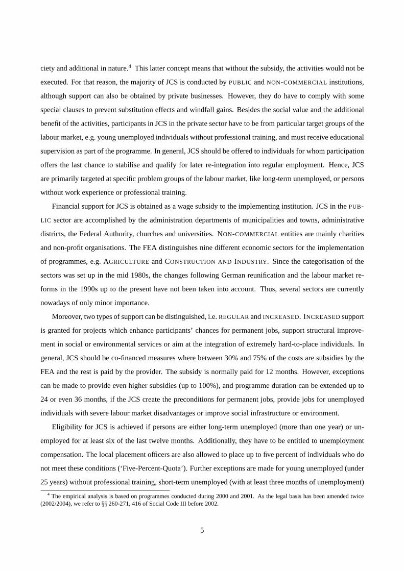
to the categoryOTHER. This leaves us with five sectors for the analysis. Figure 1 presents the number of

participants in these sectors in West and East Germany. To allow a reasonable estimation and interpretation

of treatment effects, groups with less than 100 participants are excluded from analysis. This is relevant for

women in West Germany participating in the sectorsAGRICULTURE (41) andCONSTRUCTION AND INDUS-

TRY (36). Leaving participants in the sectorOTHER aside, the majority of men in both regions participate in

sectorsAGRICULTURE (584 participants in West Germany / 925 in East Germany) andCONSTRUCTION AND

INDUSTRY (317/416). The smallest share of male participants is employed inOFFICE AND SERVICES’ occu-

pations. On the one hand, this may be due to specific abilities needed for these kind of jobs, which most of the

participants may not have. On the other hand, this may also be due to the fact that occupations in this sector

tend not to be additional in nature or of value to society. As these are the preconditions for the approval of JCS

(see Section 2), this would explain the relatively low share of participants in this sector. The largest share of

female participants in both parts can be found in the sectorCOMMUNITY SERVICES, with 503 participants in

West Germany and 1,810 participants in East Germany. In contrast to West Germany, female participants in

East Germany are quite often employed inAGRICULTURE. Similar to the West, the smallest group are women

in CONSTRUCTION AND INDUSTRY. This first glance already shows significant differences in the allocation

to the different sectors, not only between the regions but also between men and women.

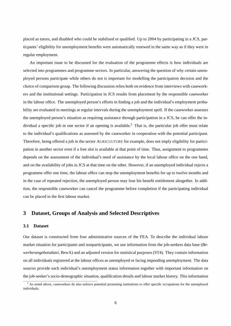
Figure 2 further differentiates the number of participants in the different sectors by type of support and

provider. Comparing the shares of participants receivingREGULAR and INCREASED support (left-hand side

of the figure) shows notable differences between East and West Germany and reflects the worse labour market

situation in East Germany. While in West Germany the majority of programmes (over 70%) is implemented

8

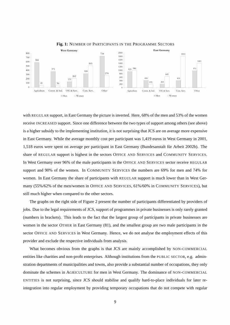
Fig. 1: NUMBER OF PARTICIPANTS IN THE PROGRAMME SECTORS

with REGULAR support, in East Germany the picture is inverted. Here, 68% of the men and 53% of the women

receiveINCREASEDsupport. Since one difference between the two types of support among others (see above)

is a higher subsidy to the implementing institution, it is not surprising that JCS are on average more expensive

in East Germany. While the average monthly cost per participant was 1,419 euros in West Germany in 2001,

1,518 euros were spent on average per participant in East Germany (Bundesanstalt fur Arbeit 2002b). The

share ofREGULAR support is highest in the sectorsOFFICE AND SERVICES andCOMMUNITY SERVICES.

In West Germany over 96% of the male participants in theOFFICE AND SERVICESsector receiveREGULAR

support and 90% of the women. InCOMMUNITY SERVICES the numbers are 69% for men and 74% for

women. In East Germany the share of participants withREGULAR support is much lower than in West Ger-

many (55%/62% of the men/women inOFFICE AND SERVICES, 61%/60% inCOMMUNITY SERVICES), but

still much higher when compared to the other sectors.

The graphs on the right side of Figure 2 present the number of participants differentiated by providers of

jobs. Due to the legal requirements of JCS, support of programmes in private businesses is only rarely granted

(numbers in brackets). This leads to the fact that the largest group of participants in private businesses are

women in the sectorOTHER in East Germany (81), and the smallest group are two male participants in the

sectorOFFICE AND SERVICES in West Germany. Hence, we do not analyse the employment effects of this

provider and exclude the respective individuals from analysis.

What becomes obvious from the graphs is that JCS are mainly accomplished byNON-COMMERCIAL

entities like charities and non-profit enterprises. Although institutions from thePUBLIC SECTOR, e.g. admin-

stration departments of municipalities and towns, also provide a substantial number of occupations, they only

dominate the schemes inAGRICULTURE for men in West Germany. The dominance ofNON-COMMERCIAL

ENTITIES is not surprising, since JCS should stabilise and qualify hard-to-place individuals for later re-

integration into regular employment by providing temporary occupations that do not compete with regular

9

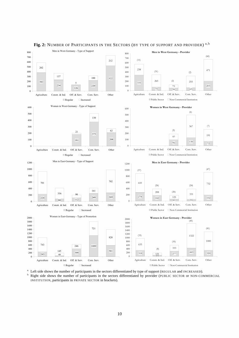
Fig. 2: NUMBER OF PARTICIPANTS IN THE SECTORS(BY TYPE OF SUPPORT AND PROVIDER) a,b

a Left side shows the number of participants in the sectors differentiated by type of support (REGULAR andINCREASED).b Right side shows the number of participants in the sectors differentiated by provider (PUBLIC SECTORor NON-COMMERCIAL

INSTITUTION, participants inPRIVATE SECTORin brackets).

10

jobs. These regulations are designed to avoid substitution effects and windfall gains and can most likely be

met by non-commercial institutions that have a sufficient demand for workers, do not compete with private

businesses and could not provide long-run opportunities for comparable employees without the subsidy.

Let us summarise so far: the occupations differ between the sectors and the implementation of schemes

differs between the two types of providers. The type of support is heterogeneous and we expect the employ-

ment effects to be heterogeneous as well. The direction of this effect heterogeneity is not clear a priori. We

have discussed already that the occupations in the different sectors differ and also require different abilities

from the participants. However, it is a priori unclear which types of occupation improve the employment

chances of individuals most. The same is true regarding the providers and also the third source of possible ef-

fect heterogeneity (the type of support), which may have numerous causes. Since one reason forINCREASED

support is a greater ‘need for assistance’, it can be argued that this type should lead to better outcomes, as

the costs are usually higher and the programme is more intense. On the other hand, it may also be claimed

that those individuals have on average worse labour market prospects. Clearly, these presumptions can be

confirmed or discarded only by empirical examination.

3.3 Selected Descriptives

Let us briefly consider the different characteristics of participants in the five sectors and compare them with

the group of nonparticipants. Tables A.1 to A.4 in the Appendix present means and frequencies of relevant

variables differentiated by gender, region and sector.7 The attributes are categorised into four types: socio-

demographic information, qualification details, labour market history, and regional context. In addition, the

average programme duration within the sectors is added. Some notable differences in this data are visible.

Whereas men in West Germany experience the shortest programme duration on average in the sectorAGRI-

CULTURE with 262 days, their counterparts in this sector in East Germany leave programmes on average after

325 days, i.e. approximately two months later. The small fraction of male participants inOFFICE AND SER-

VICES participate the longest (337 days in West Germany / 332 in East Germany). Unfortunately, our data

lacks information about the reasons for the different durations. We are unable to identify whether programme

duration is determined by the planning of the caseworkers at the beginning (nominal duration), or whether

better alternatives for the participating individuals are found during the course of the programmes (realised

duration). For women in East Germany, the average programme duration differs between sectors, too. The

participants inCONSTRUCTION AND INDUSTRY leave the programmes on average after 290 days, whereas

women inOTHER stay in programmes for almost 341 days. In contrast, programme durations for women

7 Additional statistics showing means and frequencies of relevant variables further differentiated by implementing institution andtype of support are available in the supplementary Appendix (tables C.1 to C.16).

11

in West Germany vary only minimally. They remain in programmes between 305 days (COMMUNITY SER-

VICES) and 311 days (OTHER). Apart from these sectoral differences, it has to be mentioned that participants

in West Germany remain in programmes on average for shorter periods compared to those in the East (inde-

pendently of gender). This may on the one hand be due to better alternatives on the labour market, e.g. regular

job opportunities or other ALMP programmes, or on the other hand to a different level of acceptance of the

programmes by the participants.

Let us now compare some selected characteristics of participants and nonparticipants in the different sec-

tors. A first point to note is that male nonparticipants in West Germany are, with an average age of 43 years,

significantly older than participants (at the end of January 2000). It can also be seen that the age of participants

varies considerably between the sectors. Whereas men inCONSTRUCTION AND INDUSTRY andCOMMU-

NITY SERVICESare on average about 35 years old at the begin of programmes, participants inAGRICULTURE

are already 39 and inOFFICE AND SERVICESabout 43, which almost equals the age of nonparticipants. Look-

ing at the results for women in West Germany shows a similar picture. Again nonparticipants are on average

older (43.3 years) than participants, independently of sectors. In contrast, the results for men in East Germany

show quite a different picture. Participants are on average clearly older than the nonparticipants. The youngest

participants (approximately 43 years old) are employed inCOMMUNITY SERVICES and CONSTRUCTION

AND INDUSTRY, the oldest inAGRICULTURE (46 years) andOFFICE AND SERVICES(49 years), whereas the

nonparticipants are on average 42 years old. Women in East Germany are the most homogeneous group with

respect to the ages of participants and nonparticipants. Age varies slightly between 43 years (CONSTRUCTION

AND INDUSTRY, AGRICULTURE andOTHER) and 45 years (OFFICE AND SERVICES) for participants and is

on average 44 years for nonparticipants. Except for women in West Germany, participants inOFFICE AND

SERVICESare the oldest in comparison to the other sectors. Although the individual’s age may be expected to

be an important determinant for a possible re-integration into regular employment and therefore an increasing

age should correspond to a longer programme duration, this expectation is only partly confirmed by the data.

There is a tendency that programmes last on average longer if participants are older, but no clear pattern can be

revealed. With respect to health restrictions, we find that men without health restrictions are overrepresented

in the sectorsAGRICULTURE andCONSTRUCTION AND INDUSTRY when compared to nonparticipants. This

is intuitively understandable since occupations in these sectors may involve some form of manual labour.

It is quite interesting to look at the professional training of individuals in the different sectors. Participants

without completed professional training are overrepresented in the sectorsAGRICULTURE andCONSTRUC-

TION AND INDUSTRY, whereas individuals with higher degrees are overrepresented in the sectorsOFFICE

AND SERVICES andCOMMUNITY SERVICES. Both points are true irrespective of gender and region, even

though the first point is less pronounced in East Germany. This is due to the fact that most of the individuals

12

in East Germany have at least some formal degree (‘industrial training’). Clearly, this has also to be seen in

relation to the higher age of participants in East Germany. The professional rank points in the same direction.

Men in West Germany who are white-collar workers are overrepresented in theOFFICE AND SERVICESsector

and unskilled workers are primarily found inAGRICULTURE or CONSTRUCTION AND INDUSTRY. White-

collar females in West Germany are remarkably overrepresented inOFFICE AND SERVICESandCOMMUNITY

SERVICES. Taken together, these findings indicate that more highly qualified persons are more likely to be

found in the sectorsOFFICE AND SERVICESandCOMMUNITY SERVICES, whereas low-qualified individuals

are more likely to be inAGRICULTURE or CONSTRUCTION AND INDUSTRY. A last point to note is that

nonparticipants in West Germany have on average more work experience when compared to the participants.

In East Germany, the situation is much more balanced and no large differences in work experience between

participants and nonparticipants are visible.

These findings confirm two expectations. First, participants and nonparticipants differ remarkably in their

characteristics. Clearly, this is to be expected and highlights that a simple comparison of treated and non-

treated individuals will lead to selection bias. We will address this problem in the next section. Second,

participants in the different economic sectors of JCS also have rather different characteristics, and the estima-

tion has to take this into account properly.

4 Evaluation Approach

4.1 Matching Estimator

Our empirical analysis is based on the standard framework in the microeconometric evaluation literature, the

so-called potential outcome approach (see Roy 1951 and Rubin 1974). In this framework an individual can

choose between two states, e.g. participating in a certain labour market programme or not. For each individual,

there are two potential outcomes, whereY 1 denotes the outcome with treatment andY 0 is the outcome without

treatment. The actually observed outcome for any individuali is given by:Yi = Y 1i · Di + (1 − Di) · Y 0

i ,

whereD ∈ {0, 1} is a binary treatment indicator. The treatment effect for each individuali is defined as the

difference between the potential outcomes, i.e.∆i = Y 1i − Y 0

i . Imbens (2000) and Lechner (2001) generalise

this approach for situations where a whole range of treatments is available. Although JCS comprise activities

in very different economic sectors, the discussion in section 2 has shown that potential participants are exposed

to a specific job in one sector only. Therefore, we do not need to consider the effects of a programme in one

sector relative to another, but only in comparison to nonparticipation.8 Hence, we can restrict our description

8 The description of the allocation mechanism above has shown that unemployed individuals do not have an opportunity to choosebetween different jobs in JCS since occupations are offered in line with the qualification and needs of the individual.

13

to the binary case.

The parameter of interest is the average effect of treatment on the treated (ATT), defined as:

ATT = E(∆ | D = 1) = E(Y 1 | D = 1)− E(Y 0 | D = 1). (1)

Since the second term on the right-hand side is unobservable (it describes the hypothetical outcome without

treatment for those individuals who received the treatment), Eq. (1) is not identified and additional assumptions

are needed. As we work with non-experimental data, we cannot simply take the nonparticipants’ outcome

E(Y 0 | D = 0) as an approximation of the participants’ outcome had they not participated. This would

lead to selection bias, since participants and nonparticipants are selected groups that would have different

outcomes even in the absence of treatment. However, if we are able to observe all determinants that jointly

influence the participation decision and the labour market outcomes, differences in the observable attributes

between participating and nonparticipating individuals can be adjusted away. Then, treatment decision and

treatment outcomes become independent conditional on a set of covariatesX. This is the so-called conditional

independence assumption (CIA):Y 0 qD|X, whereq denotes independence.9

Given that the CIA holds and that we have access to a large group of eligible nonparticipants, the match-

ing estimator is an appealing choice. Its basic idea is to find for each participant one nonparticipant which

is similar in all relevant (observable) characteristicsX. It is well known that matching onX can become

impossible whenX is of high dimension (‘curse of dimensionality’). To deal with this dimensionality prob-

lem, Rosenbaum and Rubin (1983) suggest the use of balancing scores. For participants and nonparticipants

with the same balancing score, the distributions of the covariatesX are the same, i.e. they are balanced across

the groups. The propensity scoreP (X), i.e. the probability of participating in a programme is one possible

balancing score, which summarises the information of the observed covariatesX into a single index func-

tion. Rosenbaum and Rubin (1983) show that if treatment assignment is strongly ignorable givenX, it is also

strongly ignorable given any balancing score. Hence, it is sufficient to assume that:Y 0 qD|P (X). In order

to find comparable non-treated individuals for all treated observations it is usually additionally assumed that

Pr(D = 1 | X) < 1, for all X. Several matching procedures have been suggested in the literature.10 We

tested the sensitivity of the estimates with respect to the algorithm choice (see Caliendo, Hujer and Thom-

sen 2005). It turns out that the results are not sensitive to this choice for our dataset and that nearest-neighbour

(NN) matching with an additional calliper of 0.02 is the most favourable choice.11 Given the large sample of

nonparticipants, we additionally match ‘without replacement’.

9 It should be noted that we only require the nonparticipating outcome to be independent of the participation decision conditionalonX to estimate ATT.

10 Good overviews can be found inHeckman, Ichimura, Smith and Todd(1998),Smith and Todd(2005) andImbens(2004). Forcalliper matching seeCochran and Rubin(1973).

11 Matching has been implemented using the Stata module psmatch2 byLeuven and Sianesi(2003).

14

4.2 Plausibility of the CIA and Comparison Group

Clearly, the CIA is in general a very strong assumption and the applicability of the matching estimator depends

crucially on the plausibility of the CIA. Hence, we will discuss and justify the plausibility of the CIA in our

context in this section. Blundell, Dearden and Sianesi (2004) argue that the plausibility of such an assumption

should always be discussed on a case-by-case basis, thereby taking account of the informational richness of

the data. Implementation of matching estimators requires choosing a set of variables that credibly justify the

CIA. Only variables that simultaneously influence the participation decision and the outcome variable should

be included in the matching procedure. Hence, economic theory, a sound knowledge of previous research

and also information about the institutional settings should guide the researcher in specifying the model (see

e.g. Smith and Todd 2005 or Sianesi 2004). Both economic theory and previous empirical findings highlight

the importance of socio-demographic and qualificational variables. Regarding the first category we can use

variables such as age, marital status, number of children, nationality (German or foreigner) and health restric-

tions. The second class (qualification variables) refers to the human capital of the individual which is also a

crucially important determinant of labour market prospects. The attributes available are professional training,

occupational group, professional rank, and work experience of the individual. Furthermore, as pointed out by

Heckman and Smith (1999), unemployment dynamics and the labour market history play a major role in driv-

ing outcomes and programme participation. Hence, we use career variables describing the individual’s labour

market history, such as the duration of the last employment, the duration of unemployment at the end of Jan-

uary 2000, the number of (unsuccessful) placement propositions, the last contact to the job center and whether

the individual plans to take part in vocational rehabilitation or has already participated in a programme before.

Heckman, Ichimura, Smith and Todd (1998) additionally emphasise the importance of drawing treated and

comparison people from the same local labour market and giving them the same questionnaire. Since we use

administrative data from the same sources for participants and nonparticipants, the latter point is a given in

our analysis. To account for the local labour market situation we use the regional context variables described

above.

Finally, the institutional structure and the selection process into JCS provide some further guidance in

selecting the relevant variables. As we have seen from the discussion in Section 2, JCS are in general open to

all job-seekers who meet the eligibility criteria. However, what should have become clear is that participation

in programmes depends on the individual’s need for assistance as evaluated by the responsible caseworker and

on the availability of a free slot in the particular sector that fits the individual’s characteristics. Caseworkers

assess the individual’s need for assistance based on the set of socio-demographic, qualificational, and career

variables used in our analysis. In addition, we are able to use the caseworkers’ subjective assessments of the

15

individuals’ placement restrictions as well. Based on the overall very informative dataset, we argue henceforth

that the CIA holds in our setting.12

Choosing a proper comparison group is the next thing to do. Although participation in ALMP programmes

is not mandatory in Germany, the majority of unemployed persons join a programme after some time. Thus,

comparing participants to individuals who will never participate is inadequate, since it can be assumed that

the latter group is particularly selective.13 Sianesi (2004) discusses this problem for Sweden and argues that

these persons are the ones who do not enter a programme because they have already found a job. Therefore,

we restrict our comparison group to those who are unemployed and eligible at the end of January 2000 and

not participating in February 2000 (but may possibly join a programme later).14 The ratio of participants to

nonparticipants in February 2000 in our data is 1:20.

4.3 Propensity Score Estimation

As we want to evaluate the impacts of participation in JCS in a specific economic sector, with a specific type

of support, and with respect to the implementing institution, we have to take account of differences regarding

the assignment to programmes. For example, it has become obvious from the findings in Section 3.3 that more

highly qualified individuals are more likely to be found in the sectorsOFFICE AND SERVICESandCOMMU-

NITY SERVICES, whereas lower-qualified ones are more likely to be inAGRICULTURE or CONSTRUCTION

AND INDUSTRY. Hence, it can be expected that the attribute ‘professional training’ has a different influence

on the participation probability in the different sectors. Thus, we estimate the propensity scores separately

for every treatment group in analysis against the group of nonparticipants. To do so, we use binary logit

models.15 To abbreviate documentation of the propensity score estimations, we only discuss the results for

the five sectors in the following.16

The results for the propensity score estimations for the five sectors can be found in Tables A.5 (Men)

and A.6 (Women) for West Germany as well as in Tables A.7 (Men) and A.8 (Women) for East Germany in

the appendix. We see immediately that the parameters of the choice estimations differ not only with respect

12 In Caliendo, Hujer and Thomsen(2005) we have also tested the sensitivity of the results to unobserved heterogeneity. The resultsturned out to be robust, indicating that the data used is in fact informative enough to base the analysis on the CIA.

13 Furthermore, it should be noted that using individuals who are observed to never participate in the programmes as the comparisongroup may invalidate the conditional independence assumption due to a conditioning on future outcomes (see the discussion inFredriksson and Johansson(2004)).

14 Tables C.21 and C.22 in the supplementary Appendix provide information on the labour market destinations during the observa-tion period of the nonparticipating individuals in February 2000. It becomes obvious that during the observation period only a minorpart of these individuals participate in ALMP programmes (about 4.5% (3.4%) of the male (female) nonparticipants in West Germanyand about 8.3% (7.8%) in East Germany in December 2002).

15 As we exclude groups of less than 100 participating individuals, we estimate 18 logit models for the five sectors, 29 logit modelsfor the five sectors with respect to the type of support, and 26 logit models for the five sectors with respect to the type of provider. Forall groups in consideration we estimate the models with respect to region and gender separately.

16 The results of the estimations for the other groups (type of support, type of provider) are available on request by the authors.

16

to regional and gender-specific differences, but also with respect to sector-specific aspects. Clearly, this has

been expected based on the descriptive analysis. For example, married men (0.6680) and women (0.1677) in

East Germany have a higher probability to join a programme in the sectorCOMMUNITY SERVICES than men

(-0.2582/ insignificant) and women (-0.4877) in the West. A good example of sector-specific differences is

the individuals’ age. Whereas age has a negative impact on the probability for men in West Germany to join

CONSTRUCTION AND INDUSTRY (-0.1343), it has a positive effect for them to joinOFFICE AND SERVICES

(0.3791). Clearly, there are also variables that influence participation probabilities irrespective of gender and

region. For example, the number of placement propositions increases the participation probabilities for men

and women in both parts and all sectors. Moreover, there is a strong tendency for men and women with

health restrictions to participate in the sectorsOFFICE AND SERVICES or COMMUNITY SERVICES when

compared to individuals without health restrictions. This makes sense, as it is not very likely for people

with health problems to work in the sectorsAGRICULTURE or CONSTRUCTION AND INDUSTRY. People

with higher qualifications tend to go into the sectorsOFFICE AND SERVICES andCOMMUNITY SERVICES,

too. For example the coefficient for West German men with a college or university degree to join the sector

OFFICE AND SERVICES is 1.5608, whereas this characteristic reduces the probability to joinAGRICULTURE

(-1.2767). The influence of professional rank works in the same direction. Individuals with a higher rank

(compared to unskilled workers) are less likely to participate inAGRICULTURE (and to a certain extent also

CONSTRUCTION AND INDUSTRY). The coefficients for the occupational groups are as expected. People who

come from service professions are also more likely to join sectorsOFFICE AND SERVICESandCOMMUNITY

SERVICESand less likely to joinAGRICULTURE andCONSTRUCTION AND INDUSTRY. No clear differences

between the sectors can be found for the unemployment duration and the duration of last employment. The

latter one decreases the participation probability for all groups in all sectors. The unemployment duration –

considered in three classes: less than 13 weeks (reference), 13 to 52 weeks and over 52 weeks – has significant

influence mainly in East Germany, where it increases the probability for nearly all sectors. Overall, it can be

stated that sector-specific differences play a major role in the participation probabilities.

4.4 Matching Quality and Common Support

Based upon the propensity score estimates and the chosen matching algorithm, we check the matching quality

by comparing the standardised bias (SB) before and after matching. Since we do not condition on all the

covariates but on the propensity scores, this is a necessary step to see if the matching procedure is able to

balance the distribution of the covariates between the group of participants and nonparticipants.17 The SB,

17 SeeCaliendo and Kopeinig(2005) for an exhaustive discussion on how to test matching quality and common support.

17

as suggested by Rosenbaum and Rubin (1985), assesses the distance in the marginal distributions of the

X-variables. For each covariateX, it is defined as the difference of the sample means in the treated and

(matched) comparison sub-samples as a percentage of the square root of the average of the sample variances

in both groups. The SB before and after matching is given by:

SB = 100 · (X1t −X0t)√0.5 · (V1t(X) + V0t(X))

, with t ∈ (0, 1). (2)

X1 (V1) is the mean (variance) in the treated group andX0 (V0) the analogue for the comparison group

before matching ift = 0, and the corresponding values after matching ift = 1. For the sake of brevity, we

calculated the means of the SB before and after matching for men and women in West and East Germany for

the different treatments in consideration as an unweighted average of all variables (mean standardised bias,

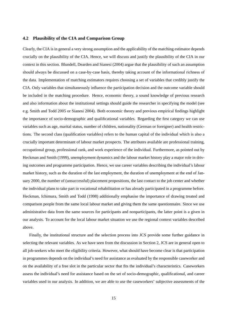
MSB). The results can be found in Table 1.

Starting with the results for the five sectors, for men in West Germany we see that the overall bias before

matching is between 14.77% (OTHER) and 23.23% (OFFICE AND SERVICES). The matching procedure is

able to achieve a significant reduction in all of the sectors and leads to a MSB after matching between 3.42%

and 4.33% for four of the five sectors.18 The MSB after matching in the sectorOFFICE AND SERVICES is still

quite high (6.86%). But taking into account that this is the smallest group of men in West Germany and that

it was reduced in size dramatically after matching, this is acceptable. For women in West Germany, the MSB

is reduced from 21.76% to 5.31% in the sectorOFFICE AND SERVICES, from 18.11% to 3.07% in the sector

COMMUNITY SERVICESand from 15.83% to 5.01% in the sectorOTHER. In East Germany the bias reduction

is even better, leaving us with a MSB after matching between 2.17% (AGRICULTURE) and 5.72% (OFFICE

AND SERVICES) for men and between 1.58% (COMMUNITY SERVICES) and 5.74% (CONSTRUCTION AND

INDUSTRY) for women. Overall, these are enormous reductions and show that the matching procedure is able

to balance the characteristics in the treatment and the matched comparison group.

Also for the further groups differentiated by type of support and implementing institution, the propensity

score specification is able to reduce the MSB after matching for most groups. However, there are some groups

for which the MSB after matching is still quite high. For example, women receiving increased support in the

sectorCOMMUNITY SERVICES in West Germany have a MSB after matching of 10.48%. This highlights the

fact that it is not always possible to find comparable individuals in the group of nonparticipants and that the

18 Additionally, we have included the standardised bias before and after matching for each variable in the main groups in tablesC.17 to C.20 in the supplementary appendix. Looking at those more detailed results shows that the matching procedure increasesthe bias for a few variables. These are in particular categorial dummy variables. For example when looking at men participatingin the AGRICULTURE sector in West Germany (table C.17), the SB in the variable ‘professional rank’ rises for the category ‘otherprofessional rank’ from 4.55% before matching to 4.82% after matching. However, this increase has to be seen in relation to the highdecrease in the other categories of this variable, e.g. the bias for ‘unskilled workers’ drops from 43.66% to 5.16%. Hence, it is onlyof minor importance.

18

Tab. 1: MEAN STANDARDISED BIAS BEFORE AND AFTER MATCHING IN

PROGRAMME SECTORS1

All Support ProviderIndividuals REGULAR INCREASED PUBLIC NON-COMM.

before after before after before after before after before afterWest GermanyMenAgriculture 18.88 3.76 19.56 4.33 19.81 5.88 19.07 5.08 18.79 5.97Construction & Industry 22.32 3.70 19.16 5.62 26.81 5.61 – – 21.18 4.62Office & Services 23.23 6.86 23.10 7.01 – – – – – –Community Services 17.89 4.33 16.86 6.10 – – – – 17.47 5.65Other 14.77 3.42 14.82 3.16 20.67 6.29 19.05 5.25 15.08 3.48WomenAgriculture – – – – – – – – – –Construction & Industry – – – – – – – – – –Office & Services 21.76 5.31 22.01 6.07 – – – – – –Community Services 18.11 3.07 18.34 3.43 22.65 10.48 19.49 7.69 18.28 3.97Other 15.83 5.01 16.63 3.81 – – – – 15.40 5.52East GermanyMenAgriculture 17.02 2.17 17.53 5.23 17.46 3.18 17.53 5.80 16.86 3.26Construction & Industry 16.65 4.02 – – 15.73 3.76 18.11 7.98 16.20 5.74Office & Services 25.43 5.72 27.60 7.93 – – – – 26.19 7.52Community Services 16.24 4.13 18.29 3.76 17.30 5.17 – – 16.36 4.97Other 11.55 3.05 17.11 4.01 11.54 3.74 13.44 6.15 11.44 3.52WomenAgriculture 18.10 2.14 16.95 5.23 17.92 2.92 17.45 5.27 18.25 3.02Construction & Industry 13.11 5.74 – – 14.17 6.10 – – 14.66 8.25Office & Services 17.62 3.02 18.18 9.94 17.13 4.70 18.13 9.47 17.50 4.10Community Services 11.81 1.58 13.46 2.37 10.77 3.20 13.86 3.83 11.58 2.05Other 11.03 2.73 13.11 3.68 12.05 2.75 13.77 3.87 10.87 3.31

1 Groups of less than 100 participants are excluded from estimation.

matching approach is limited in such situations. Fortunately, this is only the case for very few of the groups

in analysis, but has to be considered when interpreting the results.

A final aspect to bear in mind when implementing matching is the region of common support between

participants and nonparticipants. Clearly, matching estimates are only identified in the common support region

and treated individuals who fall outside this region have to be discarded. If the share of individuals lost is high,

the effects have to be re-interpreted, which might cause problems for the explanatory power of the results.

Table A.9 in the Appendix shows the number of lost treated individuals due to missing common support. For

men in West Germany, we lose between zero (CONSTRUCTION AND INDUSTRY) and 1.53% (OFFICE AND

SERVICES) of all treated individuals, which corresponds to a total loss of ten participants. For women in West

Germany, we lose seven observations and the numbers in East Germany are even lower with four men and

five women. The picture is equally good for the further groups defined by different providers and types of

support.19 Hence, common support is guaranteed and not a problem for this analysis.

19 One exception are women in West Germany participating inCOMMUNITY SERVICES receivingINCREASED support. For thisgroup we lose 14.6% of the observations. This corresponds to the finding regarding the MSB in this group and basically permits afurther interpretation of the results in this group.

19

5 Sectoral Employment Effects

5.1 Gender and Regions

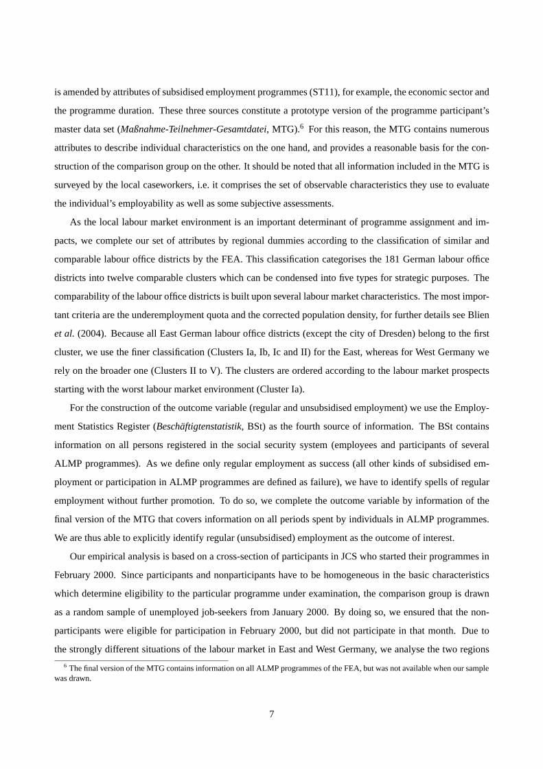
Let us start our discussion of the employment effects with the different programme sectors. The estimated

treatment effects, i.e. the differences in the employment rates between participants and matched nonpartici-

pants, are depicted in Table 2. To allow a more accurate discussion, we present the results for six selected

months only. In addition, Figures 3 and 4 contain the plots of the treatment effects over time from February

2000 to December 2002.

A first obvious finding that is common to all groups is a clear decrease in the effects shortly after pro-

grammes have started. This development is not surprising, since participants in JCS only have limited op-

portunities (and incentives) to look for regular employment whilst in the programme (‘locking-in effects). In

contrast, nonparticipants continue to search and apply for new jobs with higher intensity. However, it should

be noted that these locking-in effects vary considerably not only between the different sectors, but also be-

tween the two regions. To give an example, five months after programmes have started (July 2000), we find

significant negative employment effects for men in West Germany that range from -15.6 (AGRICULTURE)

over -23.2 (CONSTRUCTION AND INDUSTRY) to -27.2 percentage points (COMMUNITY SERVICES). This

means that the average employment rate for male participants in the sectorCOMMUNITY SERVICES is 27.2

percentage points lower compared to matched nonparticipants.

Looking at the characteristics of the participants in the different sectors might help to shed some light on

these large differences. The descriptive results (see Table A.1 in the Appendix) have shown that about 45%

of the participating men in West Germany in the sectorAGRICULTURE are unskilled workers. Additionally,

about 70% lack professional training. Taking the same figures for participants inCONSTRUCTION AND IN-

DUSTRY shows that the share of persons without professional training is larger (75%), whereas the share of

unskilled individuals is smaller (39%). However, if we compare these findings with the participants in the

sectorCOMMUNITY SERVICES, where we observe the strongest locking-in effects, we see that here the num-

ber of unskilled individuals (18%) as well as the number of persons who lack professional training (52%) are

clearly lower. Hence, the differences can (to some extent) be explained by the characteristics of individuals

allocated to the different sectors. The matched nonparticipants in the sectorAGRICULTURE are less qualified

and therefore have only limited labour market chances. Therefore, participants inAGRICULTURE experience

lower locking-in effects when compared to other sectors, such asCOMMUNITY SERVICES, where the matched

nonparticipants have on average better labour market characteristics. However, although participants in JCS

in CONSTRUCTION AND INDUSTRY have similar characteristics to the participants inAGRICULTURE, they

experience clearly stronger locking-in effects whilst in the programmes, which might be due to seasonal ef-

Tab. 2: SECTORAL EMPLOYMENT EFFECTS FORSELECTED MONTHS1

West GermanyMen

Jul 00 Dec 00 Jul 01 Dec 01 Jul 02 Dec 02Effect -0.1561 -0.0892 -0.0772-0.0223 -0.0309 0.0086AGRICULTURES.E. 0.0160 0.0166 0.0202 0.0245 0.0268 0.0256Effect -0.2318 -0.1833 -0.1321-0.0108 0.0000 0.0243CONSTRUCTION AND INDUSTRYS.E. 0.0204 0.0232 0.0300 0.0338 0.0360 0.0330Effect -0.2016 -0.2016 -0.1550-0.0853 0.0930 0.1008OFFICE AND SERVICESS.E. 0.0323 0.0315 0.0384 0.0384 0.0465 0.0486Effect -0.2722 -0.2057 -0.1203 -0.0886-0.0190 -0.0032COMMUNITY SERVICESS.E. 0.0317 0.0299 0.0333 0.0332 0.0314 0.0334Effect -0.1956 -0.1669 -0.1094 -0.0725-0.0027 0.0027OTHERS.E. 0.0163 0.0187 0.0232 0.0236 0.0246 0.0235

WomenEffect – – – – – –AGRICULTURES.E. – – – – – –Effect – – – – – –CONSTRUCTION AND INDUSTRYS.E. – – – – – –Effect -0.2289 -0.2438-0.1144 -0.0647 0.0498 0.0796OFFICE AND SERVICESS.E. 0.0289 0.0333 0.0480 0.0434 0.0448 0.0482Effect -0.1932 -0.2173 -0.1127 -0.0865-0.0020 0.0362COMMUNITY SERVICESS.E. 0.0171 0.0234 0.0270 0.0283 0.0315 0.0273Effect -0.2000 -0.2185 -0.1296-0.0926 -0.0037 0.0444OTHERS.E. 0.0249 0.0292 0.0337 0.0391 0.0423 0.0447

East GermanyMen

Effect -0.1427 -0.0984 -0.1146 -0.0605 -0.0714-0.0216AGRICULTURES.E. 0.0123 0.0124 0.0140 0.0148 0.0161 0.0148Effect -0.1947 -0.1370 -0.1298 -0.0769 -0.0841-0.0601CONSTRUCTION AND INDUSTRYS.E. 0.0173 0.0230 0.0237 0.0244 0.0217 0.0238Effect -0.1343 -0.1343 -0.1144-0.0746 -0.0249 0.0199OFFICE AND SERVICESS.E. 0.0181 0.0240 0.0334 0.0343 0.0378 0.0360Effect -0.1327 -0.1425 -0.1376 -0.0860-0.0467 -0.0319COMMUNITY SERVICESS.E. 0.0218 0.0185 0.0255 0.0253 0.0279 0.0203Effect -0.1401 -0.1205 -0.0989 -0.0639 -0.0649-0.0340OTHERS.E. 0.0105 0.0113 0.0139 0.0138 0.0149 0.0164

WomenEffect -0.0873 -0.0782 -0.0711 -0.0650 -0.0376-0.0183AGRICULTURES.E. 0.0084 0.0094 0.0125 0.0126 0.0121 0.0144Effect -0.1295 -0.0984 -0.1036-0.0207 -0.0415 0.0104CONSTRUCTION AND INDUSTRYS.E. 0.0233 0.0229 0.0310 0.0286 0.0320 0.0311Effect -0.0916 -0.0916 -0.0652 -0.0807 -0.0575 -0.0497OFFICE AND SERVICESS.E. 0.0102 0.0106 0.0174 0.0173 0.0184 0.0174Effect -0.0867 -0.0912 -0.0602 -0.0343-0.0133 0.0232COMMUNITY SERVICESS.E. 0.0063 0.0075 0.0107 0.0118 0.0126 0.0111Effect -0.1001 -0.1023 -0.0851 -0.0601 -0.0572 -0.0258OTHERS.E. 0.0087 0.0066 0.0105 0.0105 0.0111 0.0131

Bold letters indicate significance on a 1% level,italic letters refer to the 5% level, standard errorsare bootstrapped with 50 replications.Results refer to NN matching without replacement and a caliper of 0.02.1 Groups of less than 100 participants are excluded from estimation.

fects. Since our analysis starts in February, matched nonparticipants in the construction sector are more likely

to find employment during spring and summer, independent of their qualifications. Similar to the results for

men, women in West Germany experience large locking-in effects as well. In July 2000 we find negative

employment effects ranging from -19.3 (COMMUNITY SERVICES) to -22.9 percentage points (OFFICE AND

SERVICES).

21

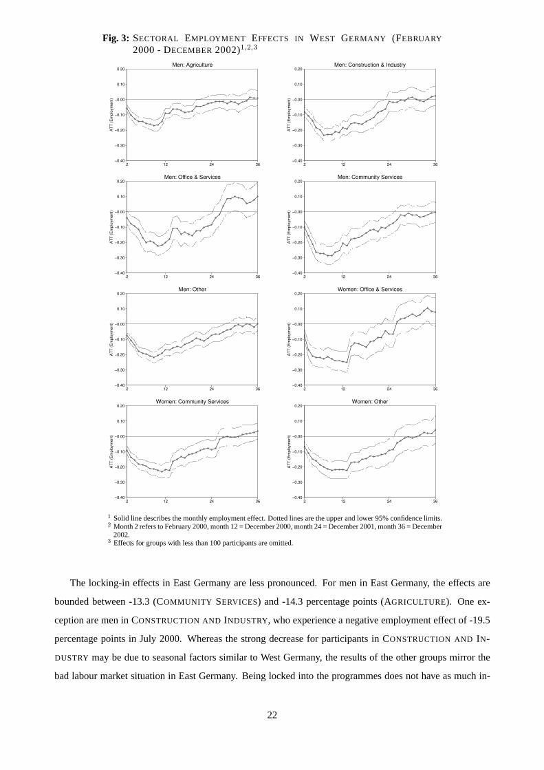
Fig. 3: SECTORAL EMPLOYMENT EFFECTS IN WEST GERMANY (FEBRUARY

2000 - DECEMBER2002)1,2,3

−0.40

−0.30

−0.20

−0.10

−0.00

0.10

0.20

AT

T (

Em

plo

ym

en

t)

2 12 24 36

Men: Agriculture

−0.40

−0.30

−0.20

−0.10

−0.00

0.10

0.20

AT

T (

Em

plo

ym

en

t)

2 12 24 36

Men: Construction & Industry

−0.40

−0.30

−0.20

−0.10

−0.00

0.10

0.20

AT

T (

Em

plo

ym

en

t)

2 12 24 36

Men: Office & Services

−0.40

−0.30

−0.20

−0.10

−0.00

0.10

0.20

AT

T (

Em

plo

ym

en

t)

2 12 24 36

Men: Community Services

−0.40

−0.30

−0.20

−0.10

−0.00

0.10

0.20

AT

T (

Em

plo

ym

en

t)

2 12 24 36

Men: Other

−0.40

−0.30

−0.20

−0.10

−0.00

0.10

0.20

AT

T (

Em

plo

ym

en

t)

2 12 24 36

Women: Office & Services

−0.40

−0.30

−0.20

−0.10

−0.00

0.10

0.20

AT

T (

Em

plo

ym

en

t)

2 12 24 36

Women: Community Services

−0.40

−0.30

−0.20

−0.10

−0.00

0.10

0.20

AT

T (

Em

plo

ym

en

t)

2 12 24 36

Women: Other

1 Solid line describes the monthly employment effect. Dotted lines are the upper and lower 95% confidence limits.2 Month 2 refers to February 2000, month 12 = December 2000, month 24 = December 2001, month 36 = December

2002.3 Effects for groups with less than 100 participants are omitted.

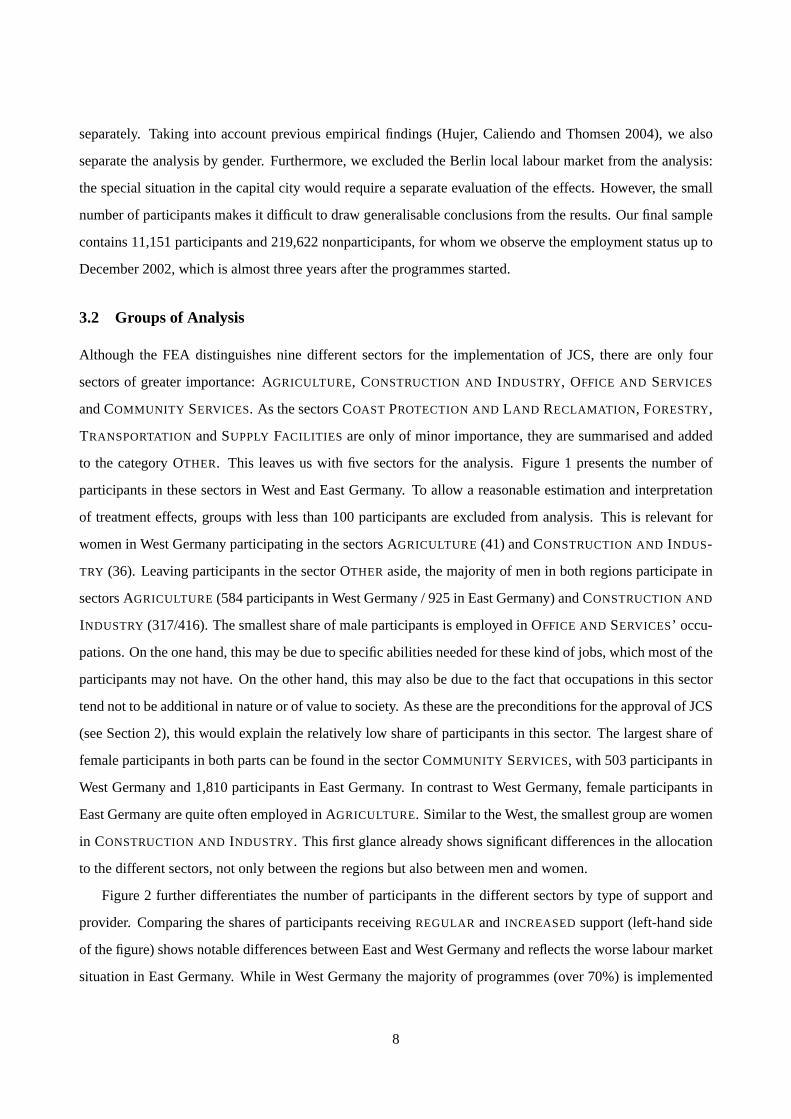
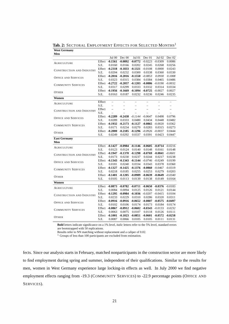
The locking-in effects in East Germany are less pronounced. For men in East Germany, the effects are

bounded between -13.3 (COMMUNITY SERVICES) and -14.3 percentage points (AGRICULTURE). One ex-

ception are men inCONSTRUCTION AND INDUSTRY, who experience a negative employment effect of -19.5

percentage points in July 2000. Whereas the strong decrease for participants inCONSTRUCTION AND IN-

DUSTRY may be due to seasonal factors similar to West Germany, the results of the other groups mirror the

bad labour market situation in East Germany. Being locked into the programmes does not have as much in-

22

fluence in terms of negative employment effects here, since the chances that nonparticipants will find a new

job are lower anyway. This seems to be valid in particular for women who experience even lower locking-in

effects compared to men in East Germany. The employment rates of participating women in July 2000 are

between -8.7 (AGRICULTURE) and -12.9 percentage points (CONSTRUCTION AND INDUSTRY) lower than

for comparable nonparticipants.

As discussed in Section 3, the average duration of the programmes is less than one year. In fact, most of

the participants leave the programmes after around 12 months. In March 2001, about 80% (74%) of the male

(female) participants in West Germany and about 91% (92%) of the male (female) participants in East Ger-

many had left the programmes. Hence, any locking-in effect should start to fade away after that time, which

is also reflected by our findings. In July 2001, the effects for all groups in both regions increased, even though

they were still significantly negative. This improvement was stronger in West Germany, where the effects in

July 2001 for men are between -7.7 (AGRICULTURE) and -15.5 percentage points (OFFICE AND SERVICES)

and for women between -11.3 (COMMUNITY SERVICES) and -12.9 percentage points (OTHER). In contrast,

the increase in the employment effects in East Germany is smaller but still observable, leading to effects for

men between -9.9 (OTHER) and -13.8 percentage points (COMMUNITY SERVICES) and for women between -

6.0 (COMMUNITY SERVICES) and -10.4 percentage points (CONSTRUCTION AND INDUSTRY) in that month.

Even though this increase is a remarkable development, the crucial question remains if participation in any

sector of JCS establishes positive employment effects.

Unfortunately, at the end of the observation period (December 2002) this is only true for two groups:

men in West Germany who participated in the sectorOFFICE AND SERVICES with an employment effect

of 10.1 and women in East Germany who participated inCOMMUNITY SERVICES with an effect of 2.3

percentage points. For all other groups, the employment effects at this point in time are still negative or at best

insignificant. In particular men in East Germany participating in the sectorsCONSTRUCTION AND INDUSTRY

andOTHER suffered from participation showing a reduction of -6.0 and -3.4 percentage points in employment

rates compared to nonparticipation. Women in East Germany who participated inOFFICE AND SERVICES

andOTHER experienced decreased employability, too, as shown by the employment effects of -5.0 and -2.6

percentage points.

These findings indicate some considerable heterogeneity in the effects of JCS with respect to the economic

sectors in which they are carried out. The overall picture is rather disappointing, however, since programmes

are not able to increase the employment rates of the participating individuals in comparison to the matched

nonparticipants. Possible explanations for this unsatisfactory outcome are the design and contents of the

programmes. Since JCS provide occupations that are additional in nature, the jobs will in general not comprise

activities that are comparable to ‘market activities’. Therefore, positive aspects in terms of human capital

23

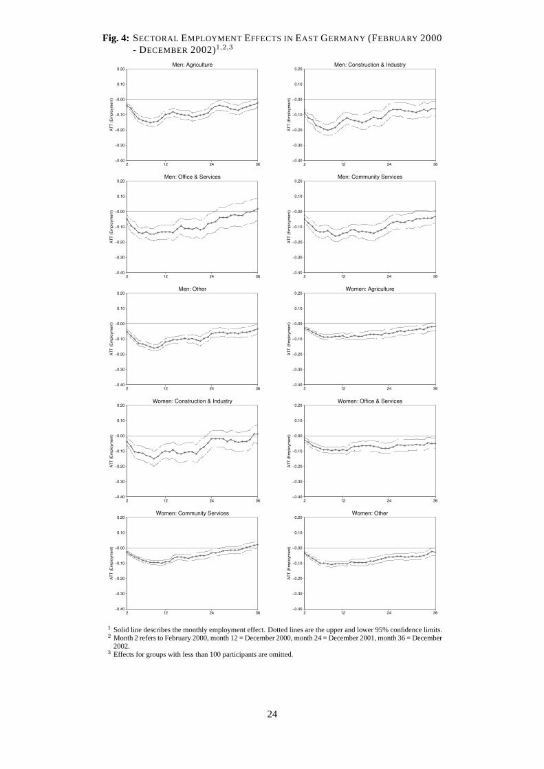
Fig. 4: SECTORAL EMPLOYMENT EFFECTS INEAST GERMANY (FEBRUARY 2000- DECEMBER2002)1,2,3

−0.40

−0.30

−0.20

−0.10

−0.00

0.10

0.20

AT

T (

Em

plo

ym

en

t)

2 12 24 36

Men: Agriculture

−0.40

−0.30

−0.20

−0.10

−0.00

0.10

0.20

AT

T (

Em

plo

ym

en

t)

2 12 24 36

Men: Construction & Industry

−0.40

−0.30

−0.20

−0.10

−0.00

0.10

0.20

AT

T (

Em

plo

ym

en

t)

2 12 24 36

Men: Office & Services

−0.40

−0.30

−0.20

−0.10

−0.00

0.10

0.20

AT

T (

Em

plo

ym

en

t)

2 12 24 36

Men: Community Services

−0.40

−0.30

−0.20

−0.10

−0.00

0.10

0.20

AT

T (

Em

plo

ym

en

t)

2 12 24 36

Men: Other

−0.40

−0.30

−0.20

−0.10

−0.00

0.10

0.20

AT

T (

Em

plo

ym

en

t)

2 12 24 36

Women: Agriculture

−0.40

−0.30

−0.20

−0.10

−0.00

0.10

0.20

AT

T (

Em

plo

ym

en

t)

2 12 24 36

Women: Construction & Industry

−0.40

−0.30

−0.20

−0.10

−0.00

0.10

0.20

AT

T (

Em

plo

ym

en

t)

2 12 24 36

Women: Office & Services

−0.40

−0.30

−0.20

−0.10

−0.00

0.10

0.20

AT

T (

Em

plo

ym

en

t)

2 12 24 36

Women: Community Services

−0.40

−0.30

−0.20

−0.10

−0.00

0.10

0.20

AT

T (

Em

plo

ym

en

t)

2 12 24 36

Women: Other

1 Solid line describes the monthly employment effect. Dotted lines are the upper and lower 95% confidence limits.2 Month 2 refers to February 2000, month 12 = December 2000, month 24 = December 2001, month 36 = December

2002.3 Effects for groups with less than 100 participants are omitted.

24

generation for the participating individuals cannot be expected in most of the sectors.

Taken together, the results (with two exceptions) are rather discouraging and confirm our previous empir-

ical findings on the effectiveness of JCS (see e.g. Hujer, Caliendo and Thomsen 2004, Caliendo, Hujer and

Thomsen 2005). Participation in the programmes does not increase the employment chances of individuals

in most cases and therefore has to be rated as a failure. What is left to examine is whether we can establish

positive effects for the two different types of support (REGULAR and INCREASED) and for the two different

providers (PUBLIC andNON-COMMERCIAL). We turn to this question in the following.

5.2 Gender, Regions and Type of Support

Tables 3 (West Germany) and 4 (East Germany) contain the employment effects in the different sectors with re-

spect to the two types of support, i.e.REGULAR andINCREASEDsupport.20 As mentioned above,INCREASED

support should be granted, e.g. for activities that improve the chances for permanent jobs or that aim at the

integration of extremely hard-to-place individuals. Therefore, particularly those individuals who have a higher

need for assistance should participate in programmes withINCREASED support.21 Hence, persons receiving

INCREASED support have on average less work experience and a correspondingly shorter last employment

duration compared to the participants receivingREGULAR support in most sectors. In addition, in particular in

West Germany, the share of persons who previously participated in ALMP programmes is clearly higher than

in theREGULAR supported groups. To give an example, whereas the share of West German male participants

receivingREGULAR support who participated before is between 18% (COMMUNITY SERVICES) and 32%

(CONSTRUCTION AND INDUSTRY), the analogues forINCREASED support range from 29% (COMMUNITY

SERVICES) to 38% (AGRICULTURE). As JCS should be offered only to persons who do not fit the require-

ments for regular employment or other ALMP programmes, the figures clearly indicate the high degree of

placement restrictions of the participants. Unfortunately, for East Germany the picture is more ambiguous.

Here, the share of persons receivingINCREASEDsupport who have participated in ALMP programmes before

is smaller in most of the groups compared to the participants receivingREGULAR support. However, these

shares are still clearly larger compared to West Germany. For men in East Germany (INCREASED support)

the shares lie between 38% (OTHER) and 51% (AGRICULTURE, CONSTRUCTION AND INDUSTRY, OFFICE

AND SERVICES), for women between 48% (CONSTRUCTION AND INDUSTRY) and 62% (OFFICE AND SER-

VICES).

Based on these differences, we expect heterogeneity in the effects, too. However, it is a priori unclear in

20 Groups of less than 100 observations have been excluded from evaluation. In the supplementary Appendix, the results over timefor the five sectors and the types of support are included (figures C.5 to C.8).

21 This higher need of assistance becomes obvious when looking at the characteristics of the participating individuals. Detailedinformation on these characteristics is given in Tables C.1, C.2, C.5, C.6, C.9, C.10, C.13 and C.14 in the supplementary Appendix.

25

which direction these effects will go. On the one hand, given that persons receivingINCREASEDsupport are

worse off in terms of their employment chances, and the programmes are designed especially for them, one

could expect stronger positive effects. On the other hand, the results for the sectors overall have shown that

JCS work rather poorly in improving the employment chances for the individuals participating. In particular,

due to the additional nature of the activities carried out, the argument may be more important that purely

maintaining contact to the labour market for the individuals participating does too little to improve their

employability. Hence, negative effects are also plausible.

Starting with the results for West Germany (Table 3) we can see the typical development of the employ-

ment effects for JCS (see above). Participants, independent of programme sector and type of support, experi-

ence negative effects in terms of regular employment shortly after programmes start. Thus, the employment

effects for July 2000 are clearly negative. Although there is some heterogeneity in the effects at this point in

time, a clear pattern that the type of support determines stronger or weaker locking-in effects could not be es-

tablished. To give an example, the effects for men receivingREGULAR support range from -15.2 (OFFICE AND

SERVICES) to -26.1 percentage points (CONSTRUCTION AND INDUSTRY) and for men receivingINCREASED

support, they lie between -20.1 (AGRICULTURE) and -24.8 percentage points (CONSTRUCTION AND INDUS-

TRY). Due to the small number of observations for women in West Germany we could not estimate the effects

for most of the sub-groups.

The same ambiguity is observable in the estimates for July 2000 for East Germany (Table 4). Whereas, for

example, male participants inAGRICULTURE are worse off when the activity isINCREASEDsupported (-16.2

percentage points) compared to male participants receivingREGULAR support (-13.8), the opposite situation

exists in the sectorCOMMUNITY SERVICES. Here, male participants receivingREGULAR support have an

employment effect of -15.7 and withINCREASEDsupport of -11.2 percentage points.

However, more important than the development of the effects during the first months after programmes

have started are the effects in the short and medium run. A further disaggregation of the effects by the type of

support shows a similar development to that described for the sectors. For all of the groups, the employment

effects increase over time. The positive employment effects in December 2002 for men in West Germany in the

sectorOFFICE AND SERVICESare also found with the further differentiation by type of support. Participants

receivingREGULAR support experience even higher employment effects with 13.6 percentage points at the

end of the observation period. Unfortunately, the group of men receivingINCREASEDsupport in this sector is

too small to allow a reasonable interpretation. For the remaining male groups in West Germany, no significant

effects could be established. For this reason, participants neither improved nor worsened their employment

rates about three years after programmes started compared to the situation had they not participated. Turning

to women in West Germany, where we could not find any significant effects in the previous section, the

26

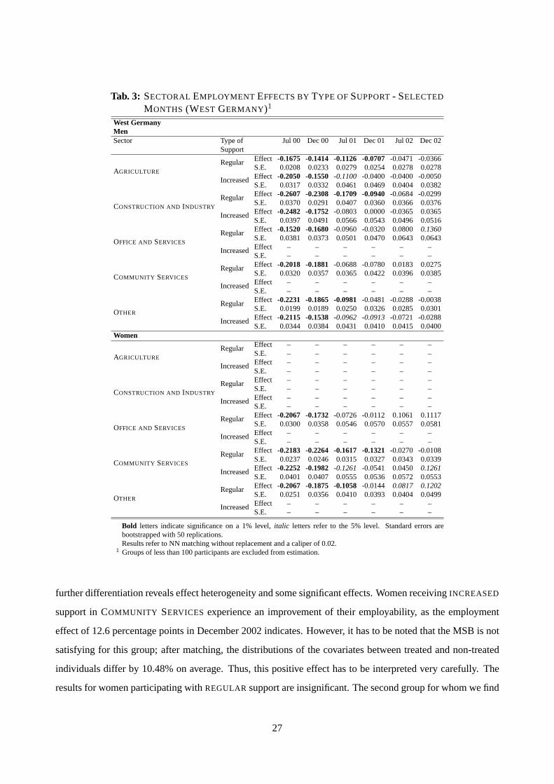
Tab. 3: SECTORAL EMPLOYMENT EFFECTS BYTYPE OFSUPPORT- SELECTED

MONTHS (WEST GERMANY)1

West GermanyMenSector Type of Jul 00 Dec 00 Jul 01 Dec 01 Jul 02 Dec 02

SupportEffect -0.1675 -0.1414 -0.1126 -0.0707-0.0471 -0.0366RegularS.E. 0.0208 0.0233 0.0279 0.0254 0.0278 0.0278AGRICULTUREEffect -0.2050 -0.1550-0.1100 -0.0400 -0.0400 -0.0050IncreasedS.E. 0.0317 0.0332 0.0461 0.0469 0.0404 0.0382Effect -0.2607 -0.2308 -0.1709 -0.0940-0.0684 -0.0299RegularS.E. 0.0370 0.0291 0.0407 0.0360 0.0366 0.0376CONSTRUCTION AND INDUSTRYEffect -0.2482 -0.1752-0.0803 0.0000 -0.0365 0.0365IncreasedS.E. 0.0397 0.0491 0.0566 0.0543 0.0496 0.0516Effect -0.1520 -0.1680-0.0960 -0.0320 0.08000.1360RegularS.E. 0.0381 0.0373 0.0501 0.0470 0.0643 0.0643OFFICE AND SERVICESEffect – – – – – –IncreasedS.E. – – – – – –Effect -0.2018 -0.1881-0.0688 -0.0780 0.0183 0.0275RegularS.E. 0.0320 0.0357 0.0365 0.0422 0.0396 0.0385COMMUNITY SERVICESEffect – – – – – –IncreasedS.E. – – – – – –Effect -0.2231 -0.1865 -0.0981-0.0481 -0.0288 -0.0038RegularS.E. 0.0199 0.0189 0.0250 0.0326 0.0285 0.0301OTHEREffect -0.2115 -0.1538-0.0962 -0.0913-0.0721 -0.0288IncreasedS.E. 0.0344 0.0384 0.0431 0.0410 0.0415 0.0400

WomenEffect – – – – – –RegularS.E. – – – – – –AGRICULTUREEffect – – – – – –IncreasedS.E. – – – – – –Effect – – – – – –RegularS.E. – – – – – –CONSTRUCTION AND INDUSTRYEffect – – – – – –IncreasedS.E. – – – – – –Effect -0.2067 -0.1732-0.0726 -0.0112 0.1061 0.1117RegularS.E. 0.0300 0.0358 0.0546 0.0570 0.0557 0.0581OFFICE AND SERVICESEffect – – – – – –IncreasedS.E. – – – – – –Effect -0.2183 -0.2264 -0.1617 -0.1321-0.0270 -0.0108RegularS.E. 0.0237 0.0246 0.0315 0.0327 0.0343 0.0339COMMUNITY SERVICESEffect -0.2252 -0.1982-0.1261 -0.0541 0.0450 0.1261IncreasedS.E. 0.0401 0.0407 0.0555 0.0536 0.0572 0.0553Effect -0.2067 -0.1875 -0.1058-0.0144 0.0817 0.1202RegularS.E. 0.0251 0.0356 0.0410 0.0393 0.0404 0.0499OTHEREffect – – – – – –IncreasedS.E. – – – – – –

Bold letters indicate significance on a 1% level,italic letters refer to the 5% level. Standard errors arebootstrapped with 50 replications.Results refer to NN matching without replacement and a caliper of 0.02.

1 Groups of less than 100 participants are excluded from estimation.

further differentiation reveals effect heterogeneity and some significant effects. Women receivingINCREASED

support inCOMMUNITY SERVICES experience an improvement of their employability, as the employment

effect of 12.6 percentage points in December 2002 indicates. However, it has to be noted that the MSB is not

satisfying for this group; after matching, the distributions of the covariates between treated and non-treated

individuals differ by 10.48% on average. Thus, this positive effect has to be interpreted very carefully. The

results for women participating withREGULAR support are insignificant. The second group for whom we find

27

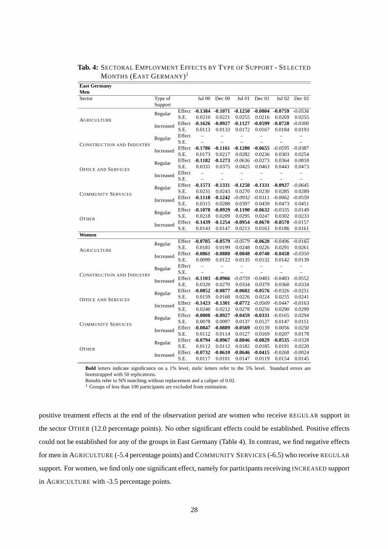
Tab. 4: SECTORAL EMPLOYMENT EFFECTS BYTYPE OFSUPPORT- SELECTED

MONTHS (EAST GERMANY)1

East GermanyMenSector Type of Jul 00 Dec 00 Jul 01 Dec 01 Jul 02 Dec 02

SupportEffect -0.1384 -0.1071 -0.1250 -0.0804 -0.0759-0.0536RegularS.E. 0.0210 0.0221 0.0255 0.0216 0.0269 0.0255AGRICULTUREEffect -0.1626 -0.0927 -0.1127 -0.0599 -0.0728-0.0300IncreasedS.E. 0.0113 0.0133 0.0172 0.0167 0.0184 0.0193Effect – – – – – –RegularS.E. – – – – – –CONSTRUCTION AND INDUSTRYEffect -0.1786 -0.1161 -0.1280 -0.0655-0.0595 -0.0387IncreasedS.E. 0.0173 0.0217 0.0282 0.0236 0.0303 0.0254Effect -0.1182 -0.1273-0.0636 -0.0273 0.0364 0.0818RegularS.E. 0.0331 0.0375 0.0425 0.0463 0.0443 0.0473OFFICE AND SERVICESEffect – – – – – –IncreasedS.E. – – – – – –Effect -0.1573 -0.1331 -0.1250 -0.1331 -0.0927-0.0645RegularS.E. 0.0231 0.0243 0.0270 0.0230 0.0285 0.0289COMMUNITY SERVICESEffect -0.1118 -0.1242-0.0932 -0.0311 -0.0062 -0.0559IncreasedS.E. 0.0315 0.0288 0.0397 0.0439 0.0473 0.0451Effect -0.1078 -0.0929 -0.1190 -0.0632-0.0335 0.0149RegularS.E. 0.0218 0.0209 0.0295 0.0247 0.0302 0.0233OTHEREffect -0.1439 -0.1254 -0.0954 -0.0670 -0.0570-0.0157IncreasedS.E. 0.0143 0.0147 0.0213 0.0163 0.0186 0.0161

WomenEffect -0.0785 -0.0579-0.0579 -0.0620 -0.0496 -0.0165RegularS.E. 0.0181 0.0199 0.0248 0.0226 0.0291 0.0261AGRICULTUREEffect -0.0861 -0.0888 -0.0848 -0.0740 -0.0458-0.0350IncreasedS.E. 0.0099 0.0122 0.0135 0.0132 0.0142 0.0139Effect – – – – – –RegularS.E. – – – – – –CONSTRUCTION AND INDUSTRYEffect -0.1103 -0.0966-0.0759 -0.0483 -0.0483 -0.0552IncreasedS.E. 0.0320 0.0270 0.0334 0.0379 0.0360 0.0334Effect -0.0852 -0.0877 -0.0602 -0.0576-0.0326 -0.0251RegularS.E. 0.0159 0.0168 0.0226 0.0224 0.0255 0.0241OFFICE AND SERVICESEffect -0.1423 -0.1301 -0.0772-0.0569 -0.0447 -0.0163IncreasedS.E. 0.0240 0.0212 0.0278 0.0256 0.0290 0.0299Effect -0.0808 -0.0927 -0.0459 -0.0331-0.0165 0.0294RegularS.E. 0.0078 0.0097 0.0137 0.0127 0.0147 0.0151COMMUNITY SERVICESEffect -0.0847 -0.0889 -0.0569-0.0139 0.0056 0.0250IncreasedS.E. 0.0112 0.0114 0.0127 0.0169 0.0207 0.0178Effect -0.0794 -0.0967 -0.0846 -0.0829 -0.0535-0.0328RegularS.E. 0.0112 0.0112 0.0182 0.0185 0.0191 0.0220OTHEREffect -0.0732 -0.0610 -0.0646 -0.0415-0.0268 -0.0024IncreasedS.E. 0.0117 0.0101 0.0147 0.0119 0.0154 0.0145

Bold letters indicate significance on a 1% level,italic letters refer to the 5% level. Standard errors arebootstrapped with 50 replications.Results refer to NN matching without replacement and a caliper of 0.02.1 Groups of less than 100 participants are excluded from estimation.

positive treatment effects at the end of the observation period are women who receiveREGULAR support in

the sectorOTHER (12.0 percentage points). No other significant effects could be established. Positive effects

could not be established for any of the groups in East Germany (Table 4). In contrast, we find negative effects

for men inAGRICULTURE(-5.4 percentage points) andCOMMUNITY SERVICES(-6.5) who receiveREGULAR

support. For women, we find only one significant effect, namely for participants receivingINCREASEDsupport

in AGRICULTURE with -3.5 percentage points.

28

Hence, we can give no clear recommendation on which type of support should be preferred. There are

only two groups with positive effects. For the first group (men inOFFICE AND SERVICES in West Germany)

we can only estimate the effects ofREGULAR support, since the number of participants receivingINCREASED

support is too small. For the second group (women inCOMMUNITY SERVICES), the findings should not be

overemphasised since the matching quality indicators (MSB and number of treated individuals lost due to

common support) are not favourable. However, for most of the groups, participation in JCS has no effect at

all.

5.3 Gender, Regions and Providers

Finally, we analyse the effect heterogeneity in the programme sectors taking into consideration the different

types of implementing institutions. As we have seen above, JCS are provided by three different types of

institutions: those in thePUBLIC sector, inNON-COMMERCIAL institutions, and inPRIVATE BUSINESSES.

Due to the small numbers of participants in JCS inPRIVATE BUSINESSES, we do not analyse these effects.

Moreover, particularly for West Germany, the differentiation by types of providers leads to numerous groups

with less than 100 participants. Hence, we are only able to evaluate the effects for six male and three female

groups. In East Germany, the differentiation is not so problematic and we have to exclude only three of the 20

possible groups.

The results for West Germany (Table 5) show that there are no clear differences with respect to locking-in

effects during the first months after participation began. For example, men inAGRICULTURE in the PUBLIC

SECTORhad an employment effect of -19.8 percentage points in July 2000, whereas those participating in a

programme provided by aNON-COMMERCIAL institution experienced a negative employment effect of -18.5

percentage point in that month. Similar results are found for male participants in the sectorOTHER (-21.9

PUBLIC/-20.5 NON-COMMERCIAL). For women inCOMMUNITY SERVICES, the relation is reversed, with

-19.8 percentage points in thePUBLIC SECTORand -21.0 percentage points in theNON-COMMERCIAL sector.

Although the effects increase in the following months, there are no significant positive effects at all at the end

of our observation period in December 2002. For this reason, no differences that are due to the implementing

institutions in the effects of JCS could be established in the different programme sectors.

Unfortunately, the situation in East Germany (Table 6) is different, but not better. Similar to the results

in the former sections, the locking-in effects are smaller in East Germany compared to the West. However,

differences between the types of providers in the sectors can be observed. For example, whereas male par-

ticipants inAGRICULTURE experience an employment effect of -14.8 percentage points if the programme is

offered by aPUBLIC provider, participants in the same sector at aNON-COMMERCIAL provider have reduced

employment rates of -12.5 percentage points. Men and women participating in the sectorCONSTRUCTION

29

Tab. 5: SECTORAL EMPLOYMENT EFFECTS BY TYPE OF PROVIDER - SELECTED

MONTHS (WEST GERMANY)1

West GermanyMenSector Provider Jul 00 Dec 00 Jul 01 Dec 01 Jul 02 Dec 02

Effect -0.1976 -0.1108 -0.1138-0.0659 -0.0449 -0.0120PublicS.E. 0.0228 0.0218 0.0239 0.0258 0.0297 0.0228AGRICULTUREEffect -0.1849 -0.1681-0.0840 -0.0378 0.0168 0.0294Non-CommercialS.E. 0.0316 0.0308 0.0337 0.0373 0.0363 0.0325Effect – – – – – –PublicS.E. – – – – – –CONSTRUCTION AND INDUSTRYEffect -0.1932 -0.1818 -0.1023-0.0379 -0.0455 -0.0076Non-CommercialS.E. 0.0274 0.0264 0.0365 0.0328 0.0356 0.0363Effect – – – – – –PublicS.E. – – – – – –OFFICE AND SERVICESEffect – – – – – –Non-CommercialS.E. – – – – – –Effect – – – – – –PublicS.E. – – – – – –COMMUNITY SERVICESEffect -0.2283 -0.2165 -0.1496 -0.1024-0.0472 0.0197Non-CommercialS.E. 0.0302 0.0329 0.0380 0.0373 0.0383 0.0362Effect -0.2189 -0.1990 -0.1592 -0.1343-0.0945 -0.0348PublicS.E. 0.0365 0.0360 0.0377 0.0366 0.0377 0.0359OTHEREffect -0.2047 -0.1599 -0.0981 -0.0661-0.0235 0.0043Non-CommercialS.E. 0.0215 0.0263 0.0252 0.0256 0.0297 0.0309

WomenEffect – – – – – –PublicS.E. – – – – – –AGRICULTUREEffect – – – – – –Non-CommercialS.E. – – – – – –Effect – – – – – –PublicS.E. – – – – – –CONSTRUCTION AND INDUSTRYEffect – – – – – –Non-CommercialS.E. – – – – – –Effect – – – – – –PublicS.E. – – – – – –OFFICE AND SERVICESEffect – – – – – –Non-CommercialS.E. – – – – – –Effect -0.1984 -0.1984 -0.1429-0.0635 -0.0079 -0.0079PublicS.E. 0.0411 0.0395 0.0446 0.0484 0.0593 0.0564COMMUNITY SERVICESEffect -0.2099 -0.2431 -0.1160 -0.09390.0138 0.0442Non-CommercialS.E. 0.0200 0.0247 0.0297 0.0326 0.0304 0.0318Effect – – – – – –PublicS.E. – – – – – –OTHEREffect -0.1937 -0.2304 -0.1257-0.0785 0.0000 0.0105Non-CommercialS.E. 0.0249 0.0355 0.0424 0.0430 0.0455 0.0454

Bold letters indicate significance on a 1% level,italic letters refer to the 5% level. Standard errors are bootstrappedwith 50 replications.Results refer to NN matching without replacement and a caliper of 0.02.

1 Groups of less than 100 participants are excluded from estimation.

AND INDUSTRY at aNON-COMMERCIAL provider experience the strongest locking-in effects, which may be

due to seasonal employment as mentioned above. Although a further improvement of the employment rates

up to the end of the observation period can be observed, most of the effects are insignificantly different from

zero in December 2002. But, it has to be noted that the effects for men in the sectorAGRICULTURE (-5.3

percentage points) as well as for women inOTHER (-3.8) accomplished byNON-COMMERCIAL providers are

significantly negative. In these two cases the activities provided byNON-COMMERCIAL institutions tend to

harm the employment chances even more than at thePUBLIC providers.

30

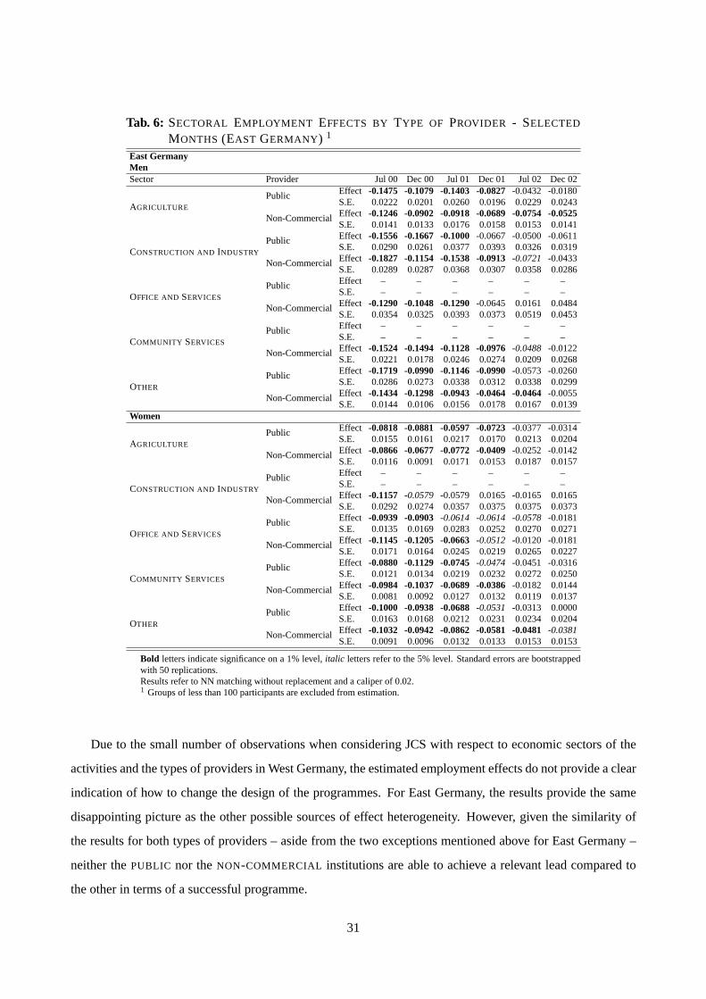
Tab. 6: SECTORAL EMPLOYMENT EFFECTS BY TYPE OF PROVIDER - SELECTED

MONTHS (EAST GERMANY) 1

East GermanyMenSector Provider Jul 00 Dec 00 Jul 01 Dec 01 Jul 02 Dec 02

Effect -0.1475 -0.1079 -0.1403 -0.0827-0.0432 -0.0180PublicS.E. 0.0222 0.0201 0.0260 0.0196 0.0229 0.0243AGRICULTUREEffect -0.1246 -0.0902 -0.0918 -0.0689 -0.0754 -0.0525Non-CommercialS.E. 0.0141 0.0133 0.0176 0.0158 0.0153 0.0141Effect -0.1556 -0.1667 -0.1000-0.0667 -0.0500 -0.0611PublicS.E. 0.0290 0.0261 0.0377 0.0393 0.0326 0.0319CONSTRUCTION AND INDUSTRYEffect -0.1827 -0.1154 -0.1538 -0.0913-0.0721 -0.0433Non-CommercialS.E. 0.0289 0.0287 0.0368 0.0307 0.0358 0.0286Effect – – – – – –PublicS.E. – – – – – –OFFICE AND SERVICESEffect -0.1290 -0.1048 -0.1290-0.0645 0.0161 0.0484Non-CommercialS.E. 0.0354 0.0325 0.0393 0.0373 0.0519 0.0453Effect – – – – – –PublicS.E. – – – – – –COMMUNITY SERVICESEffect -0.1524 -0.1494 -0.1128 -0.0976-0.0488 -0.0122Non-CommercialS.E. 0.0221 0.0178 0.0246 0.0274 0.0209 0.0268Effect -0.1719 -0.0990 -0.1146 -0.0990-0.0573 -0.0260PublicS.E. 0.0286 0.0273 0.0338 0.0312 0.0338 0.0299OTHEREffect -0.1434 -0.1298 -0.0943 -0.0464 -0.0464-0.0055Non-CommercialS.E. 0.0144 0.0106 0.0156 0.0178 0.0167 0.0139

WomenEffect -0.0818 -0.0881 -0.0597 -0.0723-0.0377 -0.0314PublicS.E. 0.0155 0.0161 0.0217 0.0170 0.0213 0.0204AGRICULTUREEffect -0.0866 -0.0677 -0.0772 -0.0409-0.0252 -0.0142Non-CommercialS.E. 0.0116 0.0091 0.0171 0.0153 0.0187 0.0157Effect – – – – – –PublicS.E. – – – – – –CONSTRUCTION AND INDUSTRYEffect -0.1157 -0.0579 -0.0579 0.0165 -0.0165 0.0165Non-CommercialS.E. 0.0292 0.0274 0.0357 0.0375 0.0375 0.0373Effect -0.0939 -0.0903-0.0614 -0.0614 -0.0578-0.0181PublicS.E. 0.0135 0.0169 0.0283 0.0252 0.0270 0.0271OFFICE AND SERVICESEffect -0.1145 -0.1205 -0.0663-0.0512 -0.0120 -0.0181Non-CommercialS.E. 0.0171 0.0164 0.0245 0.0219 0.0265 0.0227Effect -0.0880 -0.1129 -0.0745-0.0474 -0.0451 -0.0316PublicS.E. 0.0121 0.0134 0.0219 0.0232 0.0272 0.0250COMMUNITY SERVICESEffect -0.0984 -0.1037 -0.0689 -0.0386-0.0182 0.0144Non-CommercialS.E. 0.0081 0.0092 0.0127 0.0132 0.0119 0.0137Effect -0.1000 -0.0938 -0.0688-0.0531 -0.0313 0.0000PublicS.E. 0.0163 0.0168 0.0212 0.0231 0.0234 0.0204OTHEREffect -0.1032 -0.0942 -0.0862 -0.0581 -0.0481-0.0381Non-CommercialS.E. 0.0091 0.0096 0.0132 0.0133 0.0153 0.0153

Bold letters indicate significance on a 1% level,italic letters refer to the 5% level. Standard errors are bootstrappedwith 50 replications.Results refer to NN matching without replacement and a caliper of 0.02.1 Groups of less than 100 participants are excluded from estimation.

Due to the small number of observations when considering JCS with respect to economic sectors of the

activities and the types of providers in West Germany, the estimated employment effects do not provide a clear

indication of how to change the design of the programmes. For East Germany, the results provide the same

disappointing picture as the other possible sources of effect heterogeneity. However, given the similarity of

the results for both types of providers – aside from the two exceptions mentioned above for East Germany –

neither thePUBLIC nor theNON-COMMERCIAL institutions are able to achieve a relevant lead compared to

the other in terms of a successful programme.

31

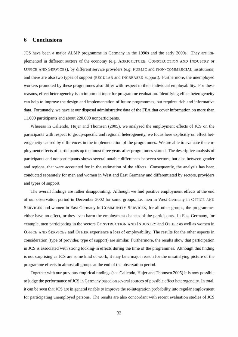
6 Conclusions

JCS have been a major ALMP programme in Germany in the 1990s and the early 2000s. They are im-

plemented in different sectors of the economy (e.g.AGRICULTURE, CONSTRUCTION AND INDUSTRY or

OFFICE AND SERVICES), by different service providers (e.g.PUBLIC andNON-COMMERCIAL institutions)

and there are also two types of support (REGULAR and INCREASED support). Furthermore, the unemployed

workers promoted by these programmes also differ with respect to their individual employability. For these

reasons, effect heterogeneity is an important topic for programme evaluation. Identifying effect heterogeneity

can help to improve the design and implementation of future programmes, but requires rich and informative

data. Fortunately, we have at our disposal administrative data of the FEA that cover information on more than

11,000 participants and about 220,000 nonparticipants.

Whereas in Caliendo, Hujer and Thomsen (2005), we analysed the employment effects of JCS on the

participants with respect to group-specific and regional heterogeneity, we focus here explicitly on effect het-

erogeneity caused by differences in the implementation of the programmes. We are able to evaluate the em-

ployment effects of participants up to almost three years after programmes started. The descriptive analysis of

participants and nonparticipants shows several notable differences between sectors, but also between gender

and regions, that were accounted for in the estimation of the effects. Consequently, the analysis has been

conducted separately for men and women in West and East Germany and differentiated by sectors, providers

and types of support.

The overall findings are rather disappointing. Although we find positive employment effects at the end

of our observation period in December 2002 for some groups, i.e. men in West Germany inOFFICE AND

SERVICES and women in East Germany inCOMMUNITY SERVICES, for all other groups, the programmes

either have no effect, or they even harm the employment chances of the participants. In East Germany, for

example, men participating in the sectorsCONSTRUCTION AND INDUSTRY andOTHER as well as women in

OFFICE AND SERVICES andOTHER experience a loss of employability. The results for the other aspects in

consideration (type of provider, type of support) are similar. Furthermore, the results show that participation

in JCS is associated with strong locking-in effects during the time of the programmes. Although this finding

is not surprising as JCS are some kind of work, it may be a major reason for the unsatisfying picture of the

programme effects in almost all groups at the end of the observation period.

Together with our previous empirical findings (see Caliendo, Hujer and Thomsen 2005) it is now possible

to judge the performance of JCS in Germany based on several sources of possible effect heterogeneity. In total,

it can be seen that JCS are in general unable to improve the re-integration probability into regular employment

for participating unemployed persons. The results are also concordant with recent evaluation studies of JCS

32

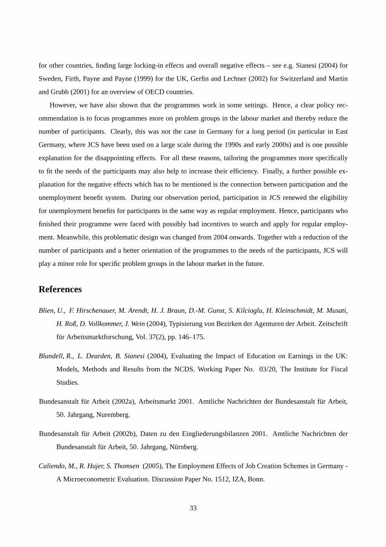
for other countries, finding large locking-in effects and overall negative effects – see e.g. Sianesi (2004) for

Sweden, Firth, Payne and Payne (1999) for the UK, Gerfin and Lechner (2002) for Switzerland and Martin

and Grubb (2001) for an overview of OECD countries.

However, we have also shown that the programmes work in some settings. Hence, a clear policy rec-

ommendation is to focus programmes more on problem groups in the labour market and thereby reduce the

number of participants. Clearly, this was not the case in Germany for a long period (in particular in East

Germany, where JCS have been used on a large scale during the 1990s and early 2000s) and is one possible

explanation for the disappointing effects. For all these reasons, tailoring the programmes more specifically

to fit the needs of the participants may also help to increase their efficiency. Finally, a further possible ex-

planation for the negative effects which has to be mentioned is the connection between participation and the

unemployment benefit system. During our observation period, participation in JCS renewed the eligibility

for unemployment benefits for participants in the same way as regular employment. Hence, participants who

finished their programme were faced with possibly bad incentives to search and apply for regular employ-

ment. Meanwhile, this problematic design was changed from 2004 onwards. Together with a reduction of the

number of participants and a better orientation of the programmes to the needs of the participants, JCS will

play a minor role for specific problem groups in the labour market in the future.

References

Blien, U., F. Hirschenauer, M. Arendt, H. J. Braun, D.-M. Gunst, S. Kilcioglu, H. Kleinschmidt, M. Musati,

H. Roß, D. Vollkommer, J. Wein(2004), Typisierung von Bezirken der Agenturen der Arbeit. Zeitschrift

fur Arbeitsmarktforschung, Vol. 37(2), pp. 146–175.

Blundell, R., L. Dearden, B. Sianesi(2004), Evaluating the Impact of Education on Earnings in the UK:

Models, Methods and Results from the NCDS. Working Paper No. 03/20, The Institute for Fiscal

Studies.

Bundesanstalt fur Arbeit (2002a), Arbeitsmarkt 2001. Amtliche Nachrichten der Bundesanstalt fur Arbeit,

50. Jahrgang, Nuremberg.

Bundesanstalt fur Arbeit (2002b), Daten zu den Eingliederungsbilanzen 2001. Amtliche Nachrichten der

Bundesanstalt fur Arbeit, 50. Jahrgang, Nurnberg.

Caliendo, M., R. Hujer, S. Thomsen(2005), The Employment Effects of Job Creation Schemes in Germany -

A Microeconometric Evaluation. Discussion Paper No. 1512, IZA, Bonn.

33

Caliendo, M., S. Kopeinig(2005), Some Practical Guidance for the Implementation of Propensity Score Match-

ing. Discussion Paper No. 1588, IZA, Bonn.

Cochran, W., D. Rubin(1973), Controlling Bias in Observational Studies. Sankyha, Vol. 35, pp. 417–446.

Eichler, M., M. Lechner(2002), An Evaluation of Public Employment Programmes in the East German State

of Sachsen-Anhalt. Labour Economics, Vol. 9, pp. 143–186.

Firth, D., C. Payne, J. Payne(1999), Efficacy of Programmes for the Unemployed: Discrete Time Modelling

of Duration Data from a Matched Comparison Study. Journal of the Royal Statistical Society, Vol.

162(1), pp. 111–120.

Fitzenberger, B., S. Speckesser(2005), Employment Effects of the Provision of Specific Professional Skills

and Techniques in Germany. Working Paper, Goethe-University Frankfurt.

Fredriksson, P., P. Johansson(2004), Dynamic Treatment Assignment - The Consequences for Evaluations

using Observational Data. Discussion Paper IFAU, Uppsala.

Gerfin, M., M. Lechner(2002), A Microeconometric Evaluation of the Active Labour Market Policy in Switzer-

land. The Economic Journal, Vol. 112, pp. 854–893.

Hubler, O. (1997), Evaluation beschaftigungspolitischer Maßnahmen in Ostdeutschland. Jahrbucher fur Na-

tionalokonomie und Statistik, Vol. 216, pp. 21–44.

Heckman, J., H. Ichimura, J. Smith, P. Todd(1998), Characterizing Selection Bias Using Experimental Data.

Econometrica, Vol. 66, pp. 1017–1098.

Heckman, J., J. Smith(1999), The Pre-Program Earnings Dip and the Determinants of Participation in a So-

cial Program: Implications for Simple Program Evaluation Strategies. Working Paper No. 6983, Na-

tional Bureau of Economic Research.

Hujer, R., M. Caliendo, S. Thomsen(2004), New Evidence on the Effects of Job Creation Schemes in Ger-

many - A Matching Approach with Threefold Heterogeneity. Research in Economics, Vol. 58(4), pp.

257–302.

Imbens, G.(2000), The Role of the Propensity Score in Estimating Dose-Response Functions. Biometrika,

Vol. 87(3), pp. 706–710.

Imbens, G.(2004), Nonparametric Estimation of Average Treatment Effects under Exogeneity: A Review.

The Review of Economics and Statistics, Vol. 86(1), pp. 4–29.

34

Kraus, F., P. Puhani, V. Steiner(2000), Do Public Works Programs Work? Some Unpleasant Results from

the East German Experience. in S. Polachek (ed.), Research in Labour Economics, JAI Press.

Lechner, M. (2001), Identification and Estimation of Causal Effects of Multiple Treatments Under the Con-

ditional Independence Assumption. in: Econometric Evaluation of Labour Market Policies, ed. by

M. Lechner,andF. Pfeiffer, Physica-Verlag, Heidelberg.

Lechner, M., R. Miquel, C. Wunsch(2005a), Long-Run Effects of Public Sector Sponsored Training in West

Germany. Discussion Paper No. 1443, IZA, Bonn.

Lechner, M., R. Miquel, C. Wunsch(2005b), The Curse and Blessing of Training the Unemployed in a Chang-

ing Economy: The Case of East Germany After Unification. Discussion Paper No. 1684, IZA, Bonn.

Leuven, E., B. Sianesi(2003), PSMATCH2: Stata Module to Perform Full Mahalanobis and Propensity Score

Matching, Common Support Graphing, and Covariate Imbalance Testing.

Software, http://ideas.repec.org/c/boc/bocode/s432001.html.

Martin, P., D. Grubb (2001), What Works and for Whom: A Review of OECD Countries Experiences with

Active Labour Market Policies. Swedish Economic Policy Review, Vol. 8, pp. 9–56.

Rosenbaum, P., D. Rubin(1983), The Central Role of the Propensity Score in Observational Studies for

Causal Effects. Biometrika, Vol. 70, pp. 41–50.

Rosenbaum, P., D. Rubin(1985), Constructing a Control Group Using Multivariate Matched Sampling Meth-

ods that Incorporate the Propensity Score. The American Statistican, Vol. 39, pp. 33–38.

Roy, A. (1951), Some Thoughts on the Distribution of Earnings. Oxford Economic Papers, Vol. 3, pp. 135–

145.

Rubin, D. (1974), Estimating Causal Effects to Treatments in Randomised and Nonrandomised Studies. Jour-

nal of Educational Psychology, Vol. 66, pp. 688–701.

Sianesi, B.(2004), An Evaluation of the Active Labour Market Programmes in Sweden. The Review of

Economics and Statistics, Vol. 86(1), pp. 133–155.

Smith, J., P. Todd(2005), Does Matching Overcome LaLonde’s Critique of Nonexperimental Estimators?

Journal of Econometrics, Vol. 125(1-2), pp. 305–353.

35

Steiner, V., F. Kraus(1995), Haben Teilnehmer an Arbeitsbeschaffungsmaßnahmen in Ostdeutschland bes-

sere Wiederbeschaftigungschancen als Arbeitslose? IAB - Beitrage zur Arbeitsmarkt- und Berufs-

forschung 192, pp. 387–423.

36

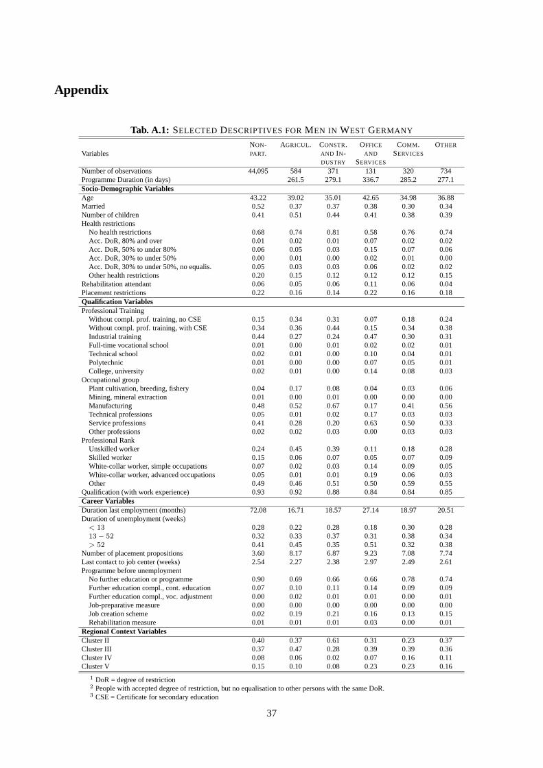
Appendix

Tab. A.1: SELECTED DESCRIPTIVES FORMEN IN WEST GERMANY

VariablesNON-PART.

AGRICUL. CONSTR.AND IN-DUSTRY

OFFICE

AND

SERVICES

COMM .SERVICES

OTHER

Number of observations 44,095 584 371 131 320 734Programme Duration (in days) 261.5 279.1 336.7 285.2 277.1Socio-Demographic VariablesAge 43.22 39.02 35.01 42.65 34.98 36.88Married 0.52 0.37 0.37 0.38 0.30 0.34Number of children 0.41 0.51 0.44 0.41 0.38 0.39Health restrictions

No health restrictions 0.68 0.74 0.81 0.58 0.76 0.74Acc. DoR, 80% and over 0.01 0.02 0.01 0.07 0.02 0.02Acc. DoR, 50% to under 80% 0.06 0.05 0.03 0.15 0.07 0.06Acc. DoR, 30% to under 50% 0.00 0.01 0.00 0.02 0.01 0.00Acc. DoR, 30% to under 50%, no equalis. 0.05 0.03 0.03 0.06 0.02 0.02Other health restrictions 0.20 0.15 0.12 0.12 0.12 0.15

Rehabilitation attendant 0.06 0.05 0.06 0.11 0.06 0.04Placement restrictions 0.22 0.16 0.14 0.22 0.16 0.18Qualification VariablesProfessional Training

Without compl. prof. training, no CSE 0.15 0.34 0.31 0.07 0.18 0.24Without compl. prof. training, with CSE 0.34 0.36 0.44 0.15 0.34 0.38Industrial training 0.44 0.27 0.24 0.47 0.30 0.31Full-time vocational school 0.01 0.00 0.01 0.02 0.02 0.01Technical school 0.02 0.01 0.00 0.10 0.04 0.01Polytechnic 0.01 0.00 0.00 0.07 0.05 0.01College, university 0.02 0.01 0.00 0.14 0.08 0.03

Occupational groupPlant cultivation, breeding, fishery 0.04 0.17 0.08 0.04 0.03 0.06Mining, mineral extraction 0.01 0.00 0.01 0.00 0.00 0.00Manufacturing 0.48 0.52 0.67 0.17 0.41 0.56Technical professions 0.05 0.01 0.02 0.17 0.03 0.03Service professions 0.41 0.28 0.20 0.63 0.50 0.33Other professions 0.02 0.02 0.03 0.00 0.03 0.03

Professional RankUnskilled worker 0.24 0.45 0.39 0.11 0.18 0.28Skilled worker 0.15 0.06 0.07 0.05 0.07 0.09White-collar worker, simple occupations 0.07 0.02 0.03 0.14 0.09 0.05White-collar worker, advanced occupations 0.05 0.01 0.01 0.19 0.06 0.03Other 0.49 0.46 0.51 0.50 0.59 0.55

Qualification (with work experience) 0.93 0.92 0.88 0.84 0.84 0.85Career VariablesDuration last employment (months) 72.08 16.71 18.57 27.14 18.97 20.51Duration of unemployment (weeks)

< 13 0.28 0.22 0.28 0.18 0.30 0.2813− 52 0.32 0.33 0.37 0.31 0.38 0.34> 52 0.41 0.45 0.35 0.51 0.32 0.38

Number of placement propositions 3.60 8.17 6.87 9.23 7.08 7.74Last contact to job center (weeks) 2.54 2.27 2.38 2.97 2.49 2.61Programme before unemployment

No further education or programme 0.90 0.69 0.66 0.66 0.78 0.74Further education compl., cont. education 0.07 0.10 0.11 0.14 0.09 0.09Further education compl., voc. adjustment 0.00 0.02 0.01 0.01 0.00 0.01Job-preparative measure 0.00 0.00 0.00 0.00 0.00 0.00Job creation scheme 0.02 0.19 0.21 0.16 0.13 0.15Rehabilitation measure 0.01 0.01 0.01 0.03 0.00 0.01

Regional Context VariablesCluster II 0.40 0.37 0.61 0.31 0.23 0.37Cluster III 0.37 0.47 0.28 0.39 0.39 0.36Cluster IV 0.08 0.06 0.02 0.07 0.16 0.11Cluster V 0.15 0.10 0.08 0.23 0.23 0.16

1 DoR = degree of restriction2 People with accepted degree of restriction, but no equalisation to other persons with the same DoR.3 CSE = Certificate for secondary education

37

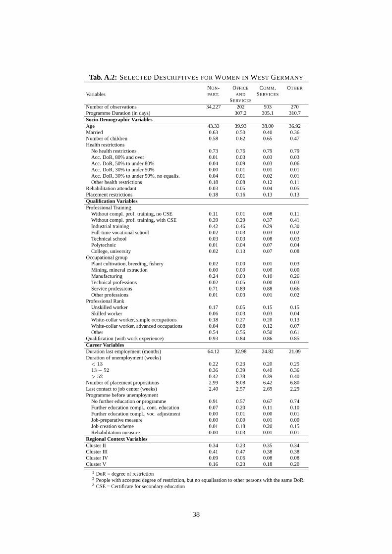
Tab. A.2: SELECTED DESCRIPTIVES FORWOMEN IN WEST GERMANY

VariablesNON-PART.

OFFICE

AND

SERVICES

COMM .SERVICES

OTHER

Number of observations 34,227 202 503 270Programme Duration (in days) 307.2 305.1 310.7Socio-Demographic VariablesAge 43.33 39.93 38.00 36.92Married 0.63 0.50 0.40 0.36Number of children 0.58 0.62 0.65 0.47Health restrictions

No health restrictions 0.73 0.76 0.79 0.79Acc. DoR, 80% and over 0.01 0.03 0.03 0.03Acc. DoR, 50% to under 80% 0.04 0.09 0.03 0.06Acc. DoR, 30% to under 50% 0.00 0.01 0.01 0.01Acc. DoR, 30% to under 50%, no equalis. 0.04 0.01 0.02 0.01Other health restrictions 0.18 0.08 0.12 0.11

Rehabilitation attendant 0.03 0.05 0.04 0.05Placement restrictions 0.18 0.16 0.13 0.13Qualification VariablesProfessional Training

Without compl. prof. training, no CSE 0.11 0.01 0.08 0.11Without compl. prof. training, with CSE 0.39 0.29 0.37 0.41Industrial training 0.42 0.46 0.29 0.30Full-time vocational school 0.02 0.03 0.03 0.02Technical school 0.03 0.03 0.08 0.03Polytechnic 0.01 0.04 0.07 0.04College, university 0.02 0.13 0.07 0.08

Occupational groupPlant cultivation, breeding, fishery 0.02 0.00 0.01 0.03Mining, mineral extraction 0.00 0.00 0.00 0.00Manufacturing 0.24 0.03 0.10 0.26Technical professions 0.02 0.05 0.00 0.03Service professions 0.71 0.89 0.88 0.66Other professions 0.01 0.03 0.01 0.02

Professional RankUnskilled worker 0.17 0.05 0.15 0.15Skilled worker 0.06 0.03 0.03 0.04White-collar worker, simple occupations 0.18 0.27 0.20 0.13White-collar worker, advanced occupations 0.04 0.08 0.12 0.07Other 0.54 0.56 0.50 0.61

Qualification (with work experience) 0.93 0.84 0.86 0.85Career VariablesDuration last employment (months) 64.12 32.98 24.82 21.09Duration of unemployment (weeks)

< 13 0.22 0.23 0.20 0.2513− 52 0.36 0.39 0.40 0.36> 52 0.42 0.38 0.39 0.40

Number of placement propositions 2.99 8.08 6.42 6.80Last contact to job center (weeks) 2.40 2.57 2.69 2.29Programme before unemployment

No further education or programme 0.91 0.57 0.67 0.74Further education compl., cont. education 0.07 0.20 0.11 0.10Further education compl., voc. adjustment 0.00 0.01 0.00 0.01Job-preparative measure 0.00 0.00 0.01 0.00Job creation scheme 0.01 0.18 0.20 0.15Rehabilitation measure 0.00 0.03 0.01 0.01

Regional Context VariablesCluster II 0.34 0.23 0.35 0.34Cluster III 0.41 0.47 0.38 0.38Cluster IV 0.09 0.06 0.08 0.08Cluster V 0.16 0.23 0.18 0.20

1 DoR = degree of restriction2 People with accepted degree of restriction, but no equalisation to other persons with the same DoR.3 CSE = Certificate for secondary education

38

Tab. A.3: SELECTED DESCRIPTIVES FORMEN IN EAST GERMANY

VariablesNON-PART.

AGRICUL. CONSTR.AND IN-DUSTRY

OFFICE

AND

SERVICES

COMM .SERVICES

OTHER

Number of observations 64788 925 416 202 410 971Programme Duration (in days) 325.0 273.5 332.1 324.3 327.1Socio-Demographic VariablesAge 41.73 46.02 43.13 48.87 42.83 43.47Married 0.48 0.54 0.51 0.73 0.58 0.50Number of children 0.36 0.42 0.45 0.40 0.40 0.37Health restrictions

No health restrictions 0.75 0.79 0.81 0.75 0.69 0.77Acc. DoR, 80% and over 0.00 0.01 0.00 0.01 0.01 0.01Acc. DoR, 50% to under 80% 0.02 0.02 0.02 0.08 0.06 0.04Acc. DoR, 30% to under 50% 0.01 0.01 0.01 0.02 0.03 0.01Acc. DoR, 30% to under 50%, no equalis. 0.02 0.02 0.01 0.03 0.02 0.01Other health restrictions 0.20 0.17 0.15 0.11 0.20 0.17

Rehabilitation attendant 0.07 0.05 0.05 0.07 0.15 0.08Placement restrictions 0.16 0.11 0.09 0.14 0.20 0.14Qualification VariablesProfessional Training

Without compl. prof. training, no CSE 0.06 0.13 0.09 0.02 0.04 0.07Without compl. prof. training, with CSE 0.17 0.19 0.19 0.11 0.18 0.24Industrial training 0.69 0.64 0.70 0.41 0.60 0.57Full-time vocational school 0.01 0.00 0.00 0.01 0.01 0.01Technical school 0.04 0.02 0.01 0.26 0.07 0.06Polytechnic 0.01 0.00 0.00 0.05 0.02 0.01College, university 0.03 0.01 0.00 0.14 0.08 0.04

Occupational groupPlant cultivation, breeding, fishery 0.05 0.13 0.06 0.03 0.02 0.04Mining, mineral extraction 0.00 0.00 0.00 0.00 0.00 0.00Manufacturing 0.53 0.56 0.72 0.13 0.42 0.53Technical professions 0.06 0.03 0.02 0.34 0.09 0.06Service professions 0.33 0.27 0.20 0.50 0.46 0.35Other professions 0.03 0.01 0.00 0.00 0.01 0.01

Professional RankUnskilled worker 0.22 0.38 0.34 0.15 0.22 0.28Skilled worker 0.29 0.20 0.23 0.15 0.21 0.19White-collar worker, simple occupations 0.04 0.02 0.02 0.18 0.07 0.06White-collar worker, advanced occupations 0.02 0.01 0.01 0.05 0.04 0.01Other 0.43 0.39 0.40 0.47 0.45 0.46

Qualification (with work experience) 0.89 0.93 0.92 0.91 0.84 0.89Career VariablesDuration last employment (months) 55.51 25.38 19.53 28.04 18.35 26.52Duration of unemployment (weeks)

< 13 0.34 0.18 0.20 0.19 0.23 0.2013− 52 0.35 0.38 0.42 0.47 0.48 0.44> 52 0.31 0.44 0.38 0.34 0.29 0.36

Number of placement propositions 3.01 5.41 6.86 7.08 6.35 6.01Last contact to job center (weeks) 2.79 2.59 2.41 2.71 2.65 2.47Programme before unemployment

No further education or programme 0.83 0.49 0.51 0.46 0.49 0.60Further education compl., cont. education 0.09 0.13 0.15 0.28 0.13 0.12Further education compl., voc. adjustment 0.03 0.06 0.06 0.04 0.06 0.04Job-preparative measure 0.00 0.00 0.00 0.00 0.01 0.00Job creation scheme 0.05 0.32 0.26 0.21 0.29 0.22Rehabilitation measure 0.01 0.00 0.00 0.02 0.01 0.01

Regional Context VariablesCluster Ia 0.22 0.35 0.15 0.24 0.11 0.22Cluster Ib 0.65 0.52 0.62 0.68 0.74 0.66Cluster Ic 0.11 0.12 0.20 0.08 0.12 0.07Cluster II 0.02 0.00 0.03 0.00 0.02 0.05

1 DoR = degree of restriction2 People with accepted degree of restriction, but no equalisation to other persons with the same DoR.3 CSE = Certificate for secondary education

39

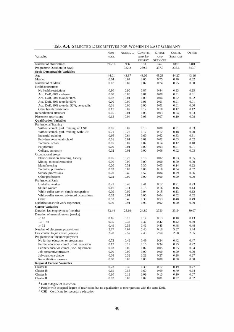
Tab. A.4: SELECTED DESCRIPTIVES FORWOMEN IN EAST GERMANY

VariablesNON-PART.

AGRICUL. CONSTR.AND IN-DUSTRY

OFFICE

AND

SERVICES

COMM .SERVICES

OTHER

Number of observations 76512 986 193 645 1810 1401Programme Duration (in days) 322.2 289.5 337.9 336.6 340.7Socio-Demographic VariablesAge 44.01 43.37 43.09 45.23 44.27 43.16Married 0.64 0.67 0.65 0.75 0.70 0.62Number of children 0.67 0.89 0.87 0.74 0.75 0.80Health restrictions

No health restrictions 0.80 0.90 0.87 0.84 0.83 0.85Acc. DoR, 80% and over 0.00 0.00 0.01 0.00 0.01 0.01Acc. DoR, 50% to under 80% 0.02 0.01 0.00 0.04 0.02 0.02Acc. DoR, 30% to under 50% 0.00 0.00 0.01 0.01 0.01 0.01Acc. DoR, 30% to under 50%, no equalis. 0.01 0.00 0.00 0.01 0.01 0.00Other health restrictions 0.17 0.09 0.12 0.10 0.12 0.12

Rehabilitation attendant 0.05 0.01 0.03 0.03 0.04 0.03Placement restrictions 0.12 0.04 0.06 0.07 0.10 0.08Qualification VariablesProfessional Training

Without compl. prof. training, no CSE 0.05 0.09 0.10 0.00 0.01 0.03Without compl. prof. training, with CSE 0.21 0.23 0.17 0.12 0.18 0.20Industrial training 0.66 0.64 0.69 0.62 0.63 0.61Full-time vocational school 0.01 0.01 0.01 0.02 0.03 0.02Technical school 0.05 0.02 0.02 0.14 0.12 0.10Polytechnic 0.00 0.01 0.00 0.03 0.01 0.01College, university 0.02 0.01 0.00 0.06 0.02 0.03

Occupational groupPlant cultivation, breeding, fishery 0.05 0.20 0.16 0.02 0.03 0.05Mining, mineral extraction 0.00 0.00 0.00 0.00 0.00 0.00Manufacturing 0.20 0.31 0.30 0.03 0.14 0.22Technical professions 0.03 0.03 0.03 0.10 0.04 0.07Service professions 0.70 0.46 0.52 0.84 0.79 0.66Other professions 0.02 0.00 0.00 0.00 0.00 0.00

Professional RankUnskilled worker 0.21 0.40 0.41 0.12 0.21 0.23Skilled worker 0.16 0.11 0.15 0.16 0.16 0.14White-collar worker, simple occupations 0.09 0.02 0.04 0.15 0.13 0.12White-collar worker, advanced occupations 0.02 0.01 0.00 0.04 0.02 0.02Other 0.53 0.46 0.39 0.53 0.48 0.49

Qualification (with work experience) 0.90 0.91 0.93 0.92 0.90 0.89Career VariablesDuration last employment (months) 63.44 25.10 24.89 37.54 33.54 30.07Duration of unemployment (weeks)

< 13 0.16 0.10 0.17 0.13 0.10 0.1313− 52 0.35 0.33 0.37 0.42 0.42 0.39> 52 0.49 0.58 0.46 0.45 0.48 0.48

Number of placement propositions 2.77 4.67 5.40 6.10 5.57 5.44Last contact to job center (weeks) 2.78 2.57 2.45 2.54 2.58 2.65Programme before unemployment

No further education or programme 0.72 0.42 0.49 0.34 0.42 0.47Further education compl., cont. education 0.17 0.19 0.16 0.34 0.25 0.22Further education compl., voc. adjustment 0.03 0.05 0.07 0.05 0.05 0.04Job-preparative measure 0.00 0.00 0.00 0.00 0.00 0.00Job creation scheme 0.08 0.33 0.28 0.27 0.28 0.27Rehabilitation measure 0.00 0.00 0.00 0.00 0.00 0.00

Regional Context VariablesCluster Ia 0.23 0.35 0.30 0.17 0.19 0.27Cluster Ib 0.65 0.53 0.60 0.69 0.70 0.64Cluster Ic 0.10 0.12 0.09 0.13 0.10 0.07Cluster II 0.02 0.00 0.02 0.01 0.02 0.02

1 DoR = degree of restriction2 People with accepted degree of restriction, but no equalisation to other persons with the same DoR.3 CSE = Certificate for secondary education

40

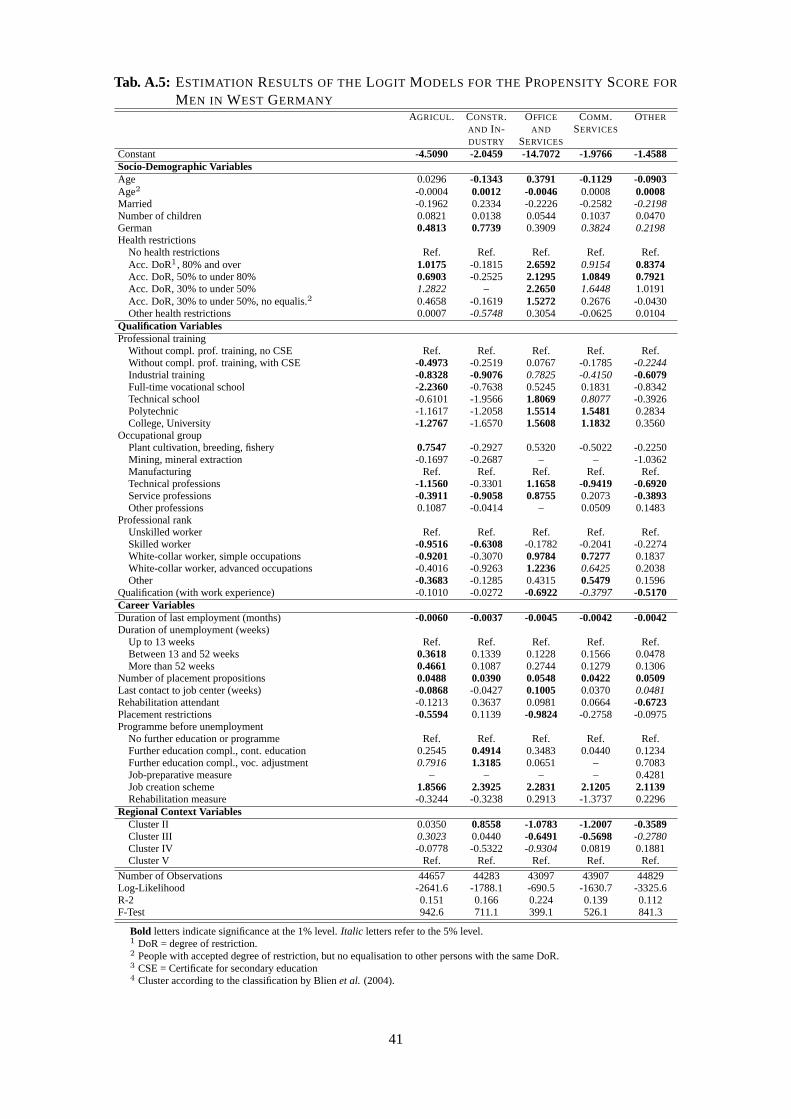
Tab. A.5: ESTIMATION RESULTS OF THELOGIT MODELS FOR THEPROPENSITYSCORE FOR

MEN IN WEST GERMANYAGRICUL. CONSTR.

AND IN-DUSTRY

OFFICE

AND

SERVICES

COMM .SERVICES

OTHER

Constant -4.5090 -2.0459 -14.7072 -1.9766 -1.4588Socio-Demographic VariablesAge 0.0296 -0.1343 0.3791 -0.1129 -0.0903Age2 -0.0004 0.0012 -0.0046 0.0008 0.0008Married -0.1962 0.2334 -0.2226 -0.2582 -0.2198Number of children 0.0821 0.0138 0.0544 0.1037 0.0470German 0.4813 0.7739 0.3909 0.3824 0.2198Health restrictions

No health restrictions Ref. Ref. Ref. Ref. Ref.Acc. DoR1, 80% and over 1.0175 -0.1815 2.6592 0.9154 0.8374Acc. DoR, 50% to under 80% 0.6903 -0.2525 2.1295 1.0849 0.7921Acc. DoR, 30% to under 50% 1.2822 – 2.2650 1.6448 1.0191Acc. DoR, 30% to under 50%, no equalis.2 0.4658 -0.1619 1.5272 0.2676 -0.0430Other health restrictions 0.0007 -0.5748 0.3054 -0.0625 0.0104

Qualification VariablesProfessional training

Without compl. prof. training, no CSE Ref. Ref. Ref. Ref. Ref.Without compl. prof. training, with CSE -0.4973 -0.2519 0.0767 -0.1785 -0.2244Industrial training -0.8328 -0.9076 0.7825 -0.4150 -0.6079Full-time vocational school -2.2360 -0.7638 0.5245 0.1831 -0.8342Technical school -0.6101 -1.9566 1.8069 0.8077 -0.3926Polytechnic -1.1617 -1.2058 1.5514 1.5481 0.2834College, University -1.2767 -1.6570 1.5608 1.1832 0.3560

Occupational groupPlant cultivation, breeding, fishery 0.7547 -0.2927 0.5320 -0.5022 -0.2250Mining, mineral extraction -0.1697 -0.2687 – – -1.0362Manufacturing Ref. Ref. Ref. Ref. Ref.Technical professions -1.1560 -0.3301 1.1658 -0.9419 -0.6920Service professions -0.3911 -0.9058 0.8755 0.2073 -0.3893Other professions 0.1087 -0.0414 – 0.0509 0.1483

Professional rankUnskilled worker Ref. Ref. Ref. Ref. Ref.Skilled worker -0.9516 -0.6308 -0.1782 -0.2041 -0.2274White-collar worker, simple occupations -0.9201 -0.3070 0.9784 0.7277 0.1837White-collar worker, advanced occupations -0.4016 -0.92631.2236 0.6425 0.2038Other -0.3683 -0.1285 0.4315 0.5479 0.1596

Qualification (with work experience) -0.1010 -0.0272 -0.6922 -0.3797 -0.5170Career VariablesDuration of last employment (months) -0.0060 -0.0037 -0.0045 -0.0042 -0.0042Duration of unemployment (weeks)

Up to 13 weeks Ref. Ref. Ref. Ref. Ref.Between 13 and 52 weeks 0.3618 0.1339 0.1228 0.1566 0.0478More than 52 weeks 0.4661 0.1087 0.2744 0.1279 0.1306

Number of placement propositions 0.0488 0.0390 0.0548 0.0422 0.0509Last contact to job center (weeks) -0.0868 -0.0427 0.1005 0.0370 0.0481Rehabilitation attendant -0.1213 0.3637 0.0981 0.0664-0.6723Placement restrictions -0.5594 0.1139 -0.9824 -0.2758 -0.0975Programme before unemployment

No further education or programme Ref. Ref. Ref. Ref. Ref.Further education compl., cont. education 0.2545 0.4914 0.3483 0.0440 0.1234Further education compl., voc. adjustment 0.7916 1.3185 0.0651 – 0.7083Job-preparative measure – – – – 0.4281Job creation scheme 1.8566 2.3925 2.2831 2.1205 2.1139Rehabilitation measure -0.3244 -0.3238 0.2913 -1.3737 0.2296

Regional Context VariablesCluster II 0.0350 0.8558 -1.0783 -1.2007 -0.3589Cluster III 0.3023 0.0440 -0.6491 -0.5698 -0.2780Cluster IV -0.0778 -0.5322 -0.9304 0.0819 0.1881Cluster V Ref. Ref. Ref. Ref. Ref.

Number of Observations 44657 44283 43097 43907 44829Log-Likelihood -2641.6 -1788.1 -690.5 -1630.7 -3325.6R-2 0.151 0.166 0.224 0.139 0.112F-Test 942.6 711.1 399.1 526.1 841.3

Bold letters indicate significance at the 1% level.Italic letters refer to the 5% level.1 DoR = degree of restriction.2 People with accepted degree of restriction, but no equalisation to other persons with the same DoR.3 CSE = Certificate for secondary education4 Cluster according to the classification by Blienet al. (2004).

41

Tab. A.6: ESTIMATION RESULTS OF THE LOGIT MODELS FOR THE

PROPENSITYSCORE FORWOMEN IN WEST GERMANYOFFICE

AND

SERVICES

COMM .SERVICES

OTHER

Constant -10.8847 -4.0484 -2.8853Socio-Demographic VariablesAge 0.1432 -0.0184 -0.0337Age2 -0.0020 -0.0001 0.0000Married -0.0555 -0.4877 -0.5266Number of children -0.0584 0.0991 -0.1484German 0.2172 0.2534 0.0660Health restrictions

No health restrictions Ref. Ref. Ref.Acc. DoR1, 80% and over 1.6533 1.2490 1.1843Acc. DoR, 50% to under 80% 1.2609 0.1901 0.8155Acc. DoR, 30% to under 50% 2.6829 1.6893 1.9266Acc. DoR, 30% to under 50%, no equalis.2 -0.1754 0.0613 -0.1396Other health restrictions -0.5043 0.0392 -0.1831

Qualification VariablesProfessional training

Without compl. prof. training, no CSE Ref. Ref. Ref.Without compl. prof. training, with CSE 1.4281 0.2030 0.1662Industrial training 1.4096 -0.1961 -0.1883Full-time vocational school 1.2480 0.0993 -0.3989Technical school 1.2967 1.0363 0.2617Polytechnic 1.9382 1.7607 1.0906College, University 2.6014 0.7199 0.9856

Occupational groupPlant cultivation, breeding, fishery – -0.3153 0.1718Mining, mineral extraction – – –Manufacturing Ref. Ref. Ref.Technical professions 2.1652 -1.5239 -0.2572Service professions 1.7365 0.7999 -0.3822Other professions 2.7255 0.3314 -0.2270

Professional rankUnskilled worker Ref. Ref. Ref.Skilled worker 0.3798 -0.3085 -0.1599White-collar worker, simple occupations 0.9857 0.0576 -0.0256White-collar worker, advanced occupations 0.6057 0.6116 0.5002Other 0.6401 -0.0642 0.3818

Qualification (with work experience) -0.5613 -0.2914 -0.2246Career VariablesDuration of last employment (months) -0.0011 -0.0036 -0.0052Duration of unemployment (weeks)

Up to 13 weeks Ref. Ref. Ref.Between 13 and 52 weeks -0.0406 0.1764 -0.0637More than 52 weeks -0.1897 0.1289 0.0470

Number of placement propositions 0.0639 0.0405 0.0519Last contact to job center (weeks) 0.0715 0.0868 -0.0107Rehabilitation attendant -0.2866 0.0587 0.4787Placement restrictions -0.2261 -0.2235 -0.4517Programme before unemployment

No further education or programme Ref. Ref. Ref.Further education compl., cont. education 1.0745 0.4635 0.1449Further education compl., voc. adjustment 0.8883 0.2137 0.7757Job-preparative measure – 3.0067 1.9089Job creation scheme 3.2762 3.0801 2.6577Rehabilitation measure 2.4833 0.4374 0.1713

Regional Context VariablesCluster II -1.1530 -0.4614 -0.4831Cluster III -0.4413 -0.4805 -0.4413Cluster IV -0.9771 -0.3191 -0.3983Cluster V Ref. Ref. Ref.

Number of Observations 33808 34722 34489Log-Likelihood -978.6 -2155.6 -1366.9Adj. R2 0.208 0.180 0.134F -Test 514.1 947.4 423.0

Bold letters indicate significance at the 1% level.Italic letters refer to the 5% level.1 DoR = degree of restriction.2 People with accepted degree of restriction, but no equalisation to other persons with the same DoR.3 CSE = Certificate for secondary education4 Cluster according to the classification by Blienet al. (2004).

42

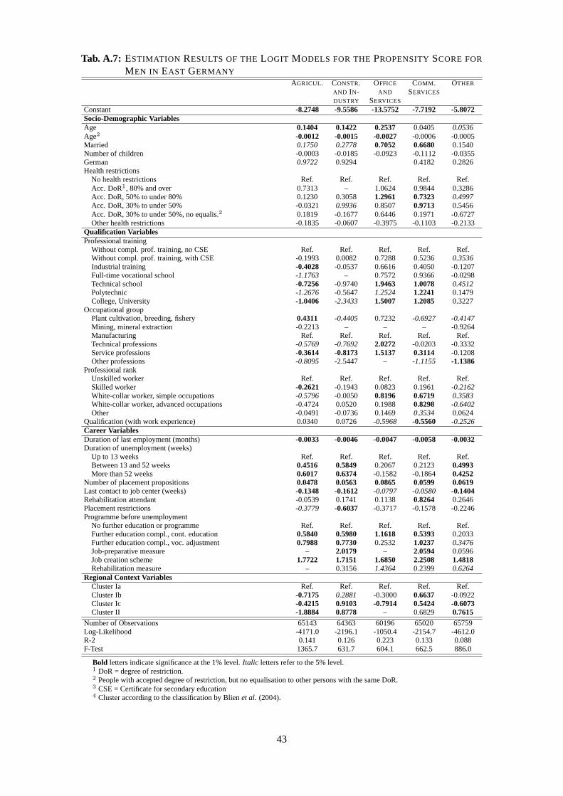
Tab. A.7: ESTIMATION RESULTS OF THELOGIT MODELS FOR THEPROPENSITYSCORE FOR

MEN IN EAST GERMANYAGRICUL. CONSTR.

AND IN-DUSTRY

OFFICE

AND

SERVICES

COMM .SERVICES

OTHER

Constant -8.2748 -9.5586 -13.5752 -7.7192 -5.8072Socio-Demographic VariablesAge 0.1404 0.1422 0.2537 0.0405 0.0536Age2 -0.0012 -0.0015 -0.0027 -0.0006 -0.0005Married 0.1750 0.2778 0.7052 0.6680 0.1540Number of children -0.0003 -0.0185 -0.0923 -0.1112 -0.0355German 0.9722 0.9294 0.4182 0.2826Health restrictions

No health restrictions Ref. Ref. Ref. Ref. Ref.Acc. DoR1, 80% and over 0.7313 – 1.0624 0.9844 0.3286Acc. DoR, 50% to under 80% 0.1230 0.3058 1.2961 0.7323 0.4997Acc. DoR, 30% to under 50% -0.0321 0.9936 0.8507 0.9713 0.5456Acc. DoR, 30% to under 50%, no equalis.2 0.1819 -0.1677 0.6446 0.1971 -0.6727Other health restrictions -0.1835 -0.0607 -0.3975 -0.1103 -0.2133

Qualification VariablesProfessional training

Without compl. prof. training, no CSE Ref. Ref. Ref. Ref. Ref.Without compl. prof. training, with CSE -0.1993 0.0082 0.7288 0.5236 0.3536Industrial training -0.4028 -0.0537 0.6616 0.4050 -0.1207Full-time vocational school -1.1763 – 0.7572 0.9366 -0.0298Technical school -0.7256 -0.9740 1.9463 1.0078 0.4512Polytechnic -1.2676 -0.5647 1.2524 1.2241 0.1479College, University -1.0406 -2.3433 1.5007 1.2085 0.3227

Occupational groupPlant cultivation, breeding, fishery 0.4311 -0.4405 0.7232 -0.6927 -0.4147Mining, mineral extraction -0.2213 – – – -0.9264Manufacturing Ref. Ref. Ref. Ref. Ref.Technical professions -0.5769 -0.7692 2.0272 -0.0203 -0.3332Service professions -0.3614 -0.8173 1.5137 0.3114 -0.1208Other professions -0.8095 -2.5447 – -1.1155 -1.1386

Professional rankUnskilled worker Ref. Ref. Ref. Ref. Ref.Skilled worker -0.2621 -0.1943 0.0823 0.1961 -0.2162White-collar worker, simple occupations -0.5796 -0.0050 0.8196 0.6719 0.3583White-collar worker, advanced occupations -0.4724 0.0520 0.19880.8298 -0.6402Other -0.0491 -0.0736 0.1469 0.3534 0.0624

Qualification (with work experience) 0.0340 0.0726 -0.5968 -0.5560 -0.2526Career VariablesDuration of last employment (months) -0.0033 -0.0046 -0.0047 -0.0058 -0.0032Duration of unemployment (weeks)

Up to 13 weeks Ref. Ref. Ref. Ref. Ref.Between 13 and 52 weeks 0.4516 0.5849 0.2067 0.2123 0.4993More than 52 weeks 0.6017 0.6374 -0.1582 -0.1864 0.4252

Number of placement propositions 0.0478 0.0563 0.0865 0.0599 0.0619Last contact to job center (weeks) -0.1348 -0.1612 -0.0797 -0.0580 -0.1404Rehabilitation attendant -0.0539 0.1741 0.1138 0.8264 0.2646Placement restrictions -0.3779 -0.6037 -0.3717 -0.1578 -0.2246Programme before unemployment

No further education or programme Ref. Ref. Ref. Ref. Ref.Further education compl., cont. education 0.5840 0.5980 1.1618 0.5393 0.2033Further education compl., voc. adjustment 0.7988 0.7730 0.2532 1.0237 0.3476Job-preparative measure – 2.0179 – 2.0594 0.0596Job creation scheme 1.7722 1.7151 1.6850 2.2508 1.4818Rehabilitation measure – 0.3156 1.4364 0.2399 0.6264

Regional Context VariablesCluster Ia Ref. Ref. Ref. Ref. Ref.Cluster Ib -0.7175 0.2881 -0.3000 0.6637 -0.0922Cluster Ic -0.4215 0.9103 -0.7914 0.5424 -0.6073Cluster II -1.8884 0.8778 – 0.6829 0.7615

Number of Observations 65143 64363 60196 65020 65759Log-Likelihood -4171.0 -2196.1 -1050.4 -2154.7 -4612.0R-2 0.141 0.126 0.223 0.133 0.088F-Test 1365.7 631.7 604.1 662.5 886.0

Bold letters indicate significance at the 1% level.Italic letters refer to the 5% level.1 DoR = degree of restriction.2 People with accepted degree of restriction, but no equalisation to other persons with the same DoR.3 CSE = Certificate for secondary education4 Cluster according to the classification by Blienet al. (2004).

43

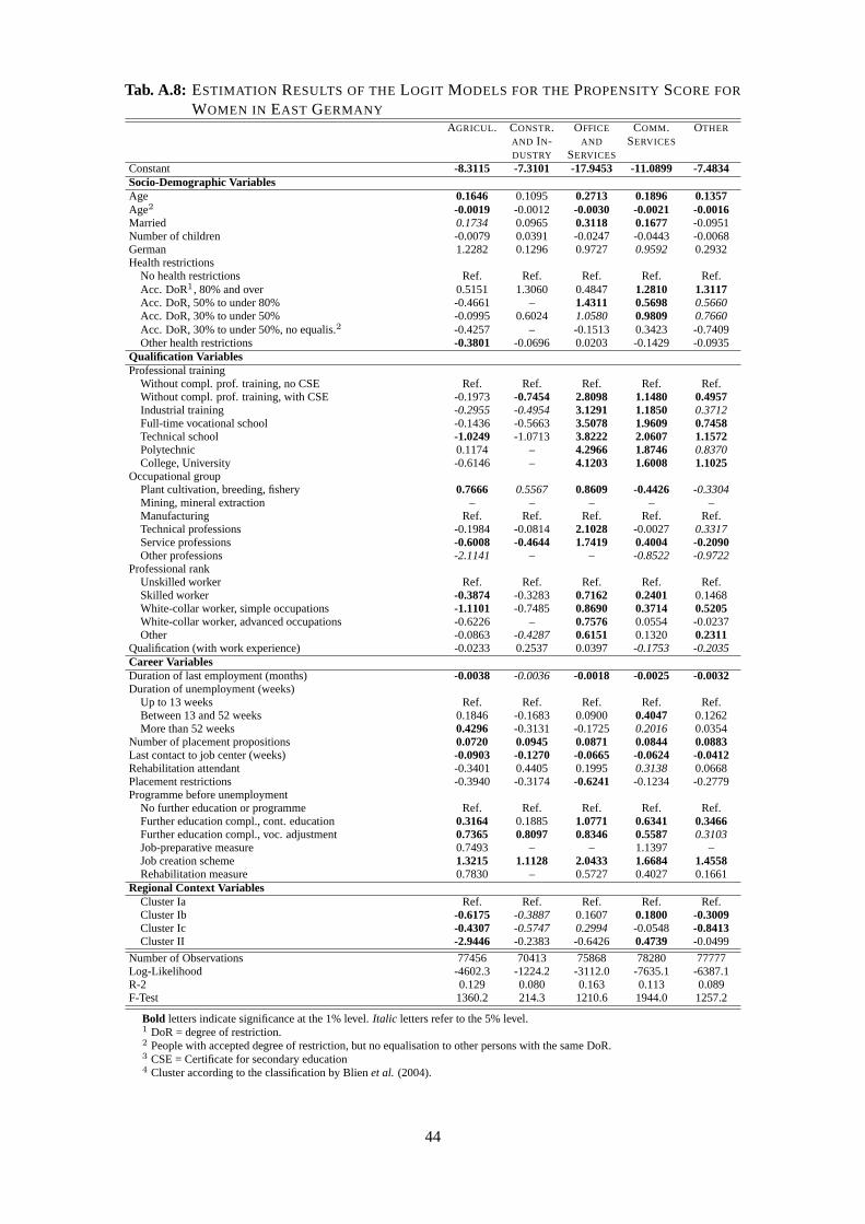
Tab. A.8: ESTIMATION RESULTS OF THELOGIT MODELS FOR THEPROPENSITYSCORE FOR

WOMEN IN EAST GERMANYAGRICUL. CONSTR.

AND IN-DUSTRY

OFFICE

AND

SERVICES

COMM .SERVICES

OTHER

Constant -8.3115 -7.3101 -17.9453 -11.0899 -7.4834Socio-Demographic VariablesAge 0.1646 0.1095 0.2713 0.1896 0.1357Age2 -0.0019 -0.0012 -0.0030 -0.0021 -0.0016Married 0.1734 0.0965 0.3118 0.1677 -0.0951Number of children -0.0079 0.0391 -0.0247 -0.0443 -0.0068German 1.2282 0.1296 0.9727 0.9592 0.2932Health restrictions

No health restrictions Ref. Ref. Ref. Ref. Ref.Acc. DoR1, 80% and over 0.5151 1.3060 0.4847 1.2810 1.3117Acc. DoR, 50% to under 80% -0.4661 – 1.4311 0.5698 0.5660Acc. DoR, 30% to under 50% -0.0995 0.6024 1.0580 0.9809 0.7660Acc. DoR, 30% to under 50%, no equalis.2 -0.4257 – -0.1513 0.3423 -0.7409Other health restrictions -0.3801 -0.0696 0.0203 -0.1429 -0.0935

Qualification VariablesProfessional training

Without compl. prof. training, no CSE Ref. Ref. Ref. Ref. Ref.Without compl. prof. training, with CSE -0.1973 -0.7454 2.8098 1.1480 0.4957Industrial training -0.2955 -0.4954 3.1291 1.1850 0.3712Full-time vocational school -0.1436 -0.5663 3.5078 1.9609 0.7458Technical school -1.0249 -1.0713 3.8222 2.0607 1.1572Polytechnic 0.1174 – 4.2966 1.8746 0.8370College, University -0.6146 – 4.1203 1.6008 1.1025

Occupational groupPlant cultivation, breeding, fishery 0.7666 0.5567 0.8609 -0.4426 -0.3304Mining, mineral extraction – – – – –Manufacturing Ref. Ref. Ref. Ref. Ref.Technical professions -0.1984 -0.0814 2.1028 -0.0027 0.3317Service professions -0.6008 -0.4644 1.7419 0.4004 -0.2090Other professions -2.1141 – – -0.8522 -0.9722

Professional rankUnskilled worker Ref. Ref. Ref. Ref. Ref.Skilled worker -0.3874 -0.3283 0.7162 0.2401 0.1468White-collar worker, simple occupations -1.1101 -0.7485 0.8690 0.3714 0.5205White-collar worker, advanced occupations -0.6226 – 0.7576 0.0554 -0.0237Other -0.0863 -0.4287 0.6151 0.1320 0.2311

Qualification (with work experience) -0.0233 0.2537 0.0397 -0.1753 -0.2035Career VariablesDuration of last employment (months) -0.0038 -0.0036 -0.0018 -0.0025 -0.0032Duration of unemployment (weeks)

Up to 13 weeks Ref. Ref. Ref. Ref. Ref.Between 13 and 52 weeks 0.1846 -0.1683 0.0900 0.4047 0.1262More than 52 weeks 0.4296 -0.3131 -0.1725 0.2016 0.0354

Number of placement propositions 0.0720 0.0945 0.0871 0.0844 0.0883Last contact to job center (weeks) -0.0903 -0.1270 -0.0665 -0.0624 -0.0412Rehabilitation attendant -0.3401 0.4405 0.1995 0.3138 0.0668Placement restrictions -0.3940 -0.3174 -0.6241 -0.1234 -0.2779Programme before unemployment

No further education or programme Ref. Ref. Ref. Ref. Ref.Further education compl., cont. education 0.3164 0.1885 1.0771 0.6341 0.3466Further education compl., voc. adjustment 0.7365 0.8097 0.8346 0.5587 0.3103Job-preparative measure 0.7493 – – 1.1397 –Job creation scheme 1.3215 1.1128 2.0433 1.6684 1.4558Rehabilitation measure 0.7830 – 0.5727 0.4027 0.1661

Regional Context VariablesCluster Ia Ref. Ref. Ref. Ref. Ref.Cluster Ib -0.6175 -0.3887 0.1607 0.1800 -0.3009Cluster Ic -0.4307 -0.5747 0.2994 -0.0548 -0.8413Cluster II -2.9446 -0.2383 -0.6426 0.4739 -0.0499

Number of Observations 77456 70413 75868 78280 77777Log-Likelihood -4602.3 -1224.2 -3112.0 -7635.1 -6387.1R-2 0.129 0.080 0.163 0.113 0.089F-Test 1360.2 214.3 1210.6 1944.0 1257.2

Bold letters indicate significance at the 1% level.Italic letters refer to the 5% level.1 DoR = degree of restriction.2 People with accepted degree of restriction, but no equalisation to other persons with the same DoR.3 CSE = Certificate for secondary education4 Cluster according to the classification by Blienet al. (2004).

44

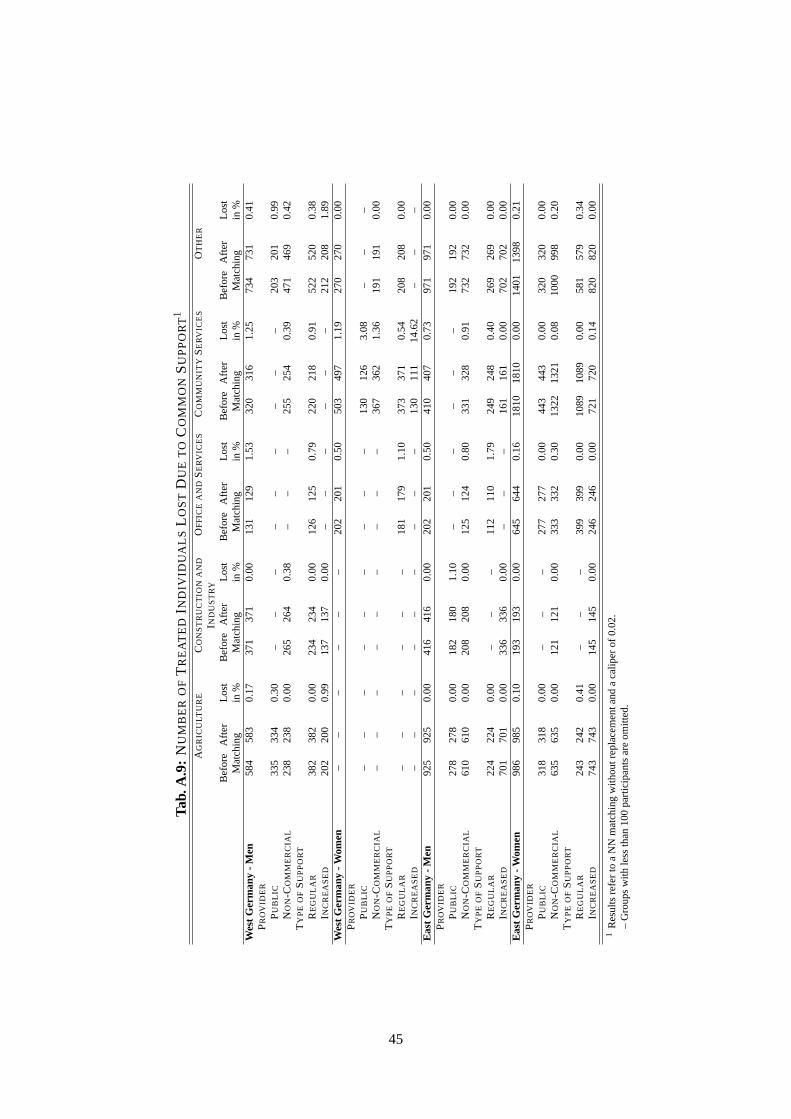
Tab.

A.9

:N

UM

BE

RO

FT

RE

AT

ED

IND

IVID

UA

LS

LO

ST

DU

ET

OC

OM

MO

NS

UP

PO

RT1

AG

RIC

ULT

UR

EC

ON

ST

RU

CT

ION

AN

D

IND

US

TR

Y

OF

FIC

EA

ND

SE

RV

ICE

SC

OM

MU

NIT

YS

ER

VIC

ES

OT

HE

R

Bef

ore

Afte

rLo

stB

efor

eA

fter

Lost

Bef

ore

Afte

rLo

stB

efor

eA

fter

Lost

Bef

ore

Afte

rLo

stM

atch

ing

in%

Mat

chin

gin

%M

atch

ing

in%

Mat

chin

gin

%M

atch

ing

in%

Wes

tGer

man

y-

Men

584

583

0.17

371

371

0.00

131

129

1.53

320

316

1.25

734

731

0.41

PR

OV

IDE

R

PU

BL

IC33

533

40.

30–

––

––

––

––

203

201

0.99

NO

N-C

OM

ME

RC

IAL

238

238

0.00

265

264

0.38

––

–25

525

40.

3947

146

90.

42T

YP

EO

FS

UP

PO

RT

RE

GU

LA

R38

238

20.

0023

423

40.

0012

612

50.

7922

021

80.

9152

252

00.

38IN

CR

EA

SE

D20

220

00.

9913

713

70.

00–

––

––

–21

220

81.

89W

estG

erm

any

-W

omen

––

––

––

202

201

0.50

503

497

1.19

270

270

0.00

PR

OV

IDE

R

PU

BL

IC–

––

––

––

––

130

126

3.08

––

–N

ON

-CO

MM

ER

CIA

L–

––

––

––

––

367

362

1.36

191

191

0.00

TY

PE

OF

SU

PP

OR

T

RE

GU

LA

R–

––

––

–18

117

91.

1037

337

10.

5420

820

80.

00IN

CR

EA

SE

D–

––

––

––

––

130

111

14.6

2–

––

Eas

tGer

man

y-

Men

925

925

0.00

416

416

0.00

202

201

0.50

410

407

0.73

971

971

0.00

PR

OV

IDE

R

PU

BL

IC27

827

80.

0018

218

01.

10–

––

––

–19

219

20.

00N

ON

-CO

MM

ER

CIA

L61

061

00.

0020

820

80.

0012

512

40.

8033

132

80.

9173

273

20.

00T

YP

EO

FS

UP

PO

RT

RE

GU

LA

R22

422

40.

00–

––

112

110

1.79

249

248

0.40

269

269

0.00

INC

RE

AS

ED

701

701

0.00

336

336

0.00

––

–16

116

10.

0070

270

20.

00E

astG

erm

any

-W

omen

986

985

0.10

193

193

0.00

645

644

0.16

1810

1810

0.00

1401

1398

0.21

PR

OV

IDE

R

PU

BL

IC31

831

80.

00–

––

277

277

0.00

443

443

0.00

320

320

0.00

NO

N-C

OM

ME

RC

IAL

635

635

0.00

121

121

0.00

333

332

0.30

1322

1321

0.08

1000

998

0.20

TY

PE

OF

SU

PP

OR

T

RE

GU

LA

R24

324

20.

41–

––

399

399

0.00

1089

1089

0.00

581

579

0.34

INC

RE

AS

ED

743

743

0.00

145

145

0.00

246

246

0.00

721

720

0.14

820

820

0.00

1R

esul

tsre

fer

toa

NN

mat

chin

gw

ithou

trep

lace

men

tand

aca

liper

of0.

02.

–G

roup

sw

ithle

ssth

an10

0pa

rtic

ipan

tsar

eom

itted

.

45

Summary (200 words):Job creation schemes (JCS) have been one important programme of active labourmarket policy (ALMP) in Germany for a long time. They aim at the re-integration of hard-to-place unem-ployed individuals into regular employment. A thorough microeconometric evaluation of these programmeswas hindered by the fact, that available survey datasets have been too small to account for a possible occur-rence of effect heterogeneity. However, identifying effect heterogeneity can help to improve the design andimplementation of future programmes. Hence, we use administrative data of the Federal Employment Agency,containing over 11,000 participants to analyse the employment effects of JCS on an individual level. We fo-cus explicitly on effect heterogeneity caused by differences in the implementation of programmes, whereas weanalysed these effects with respect to group-specific and regional heterogeneity in a previous paper. At first,we evaluate the effects with respect to the economic sector in which the JCS are accomplished. Second, weanalyse if different types of support lead to different effects. Finally, we examine if there are varying effectswhich can be attributed to different implementing institutions. The results are rather discouraging and showthat JCS are in general not able to improve the re-integration chances of participants into regular employment.

46