Sectoral Analysis of Foreign Investment and Growth In the Developed Countries

by Tam Bang Vu,

College of Business and Economics,

University of Hawaii-Hilo

tamv@hawaii.edu

and Ilan Noy,

Department of Economics,

University of Hawaii-Manoa

noy@hawaii.edu

Working Paper No. 07-25

October 2007

Abstract

Empirical studies on FDI and growth in developed countries have yielded conflicting results using cross-country regressions. We use sectoral data for a group of six country members of the Organization for Economic Cooperation and Development. Our paper is the first to identify the sector-specific impact of FDI on growth in the developed countries. Our results show that FDI might have positive or negative effect on economic growth operating directly and through its interaction with labor. Moreover, we find the effects seem to be very different across countries and economic sectors. Key Words: Foreign direct investment, growth. JEL Classification: F21, F43.

1. Introduction

During the past two decades, foreign direct investment (FDI) has become increasingly

important, with increasing volumes of direct investment flowing between and into the

developed countries recently. Figure 1 presents foreign direct investment flows into and

out of the OECD for 1992-2005. The theoretical literature in economics identifies several

channels through which FDI inflows are predicted to benefit the receiving economy. Yet,

the empirical literature has lagged behind and has had more trouble identifying these

advantages in practice. Most prominently, a large number of applied papers have looked

at the FDI-growth nexus, but their findings have been far from conclusive.1

Notwithstanding the absence of any robust conclusions, most countries continue to

vigorously pursue policies aimed at encouraging more FDI inflows.2

In this paper, we use an endogenous growth framework to estimate the impact of

FDI on growth using sectoral data for the OECD member countries. Using an augmented

production function, we let FDI directly affect GDP growth and also indirectly through

its interaction with labor. This approach creates heteroskedasticity, and so feasible

generalized least squares (FGLS) is employed. The results show that FDI has a positive

and statistically significant effect on economic growth operating both directly and

indirectly through its interaction with labor. Interestingly, the effect is not equally

distributed across economic sectors.

Our paper contributes insights on the FDI-growth nexus in several important

ways. First, we employ a country-panel fixed effects regression-based approach that

1 With the availability of better data, the last few years have seen an especially large number of empirical papers devoted to this question (e.g., Alfaro et al., 2004; Bengoa and Sanchez-Robles, 2003; Durham, 2004; Hsiao and Shen, 2003; and Li and Liu, 2005). 2 For a critical look at the fiscal revenue and spending policies targeting FDI inflows, see Hanson (2001) and Mooij and Ederveen (2003).

1

enables us to disregard variables that measure the time-invariant institutional, legal and

cultural environment in which FDI projects are implemented and which may have an

important impact on growth. These time-invariant institutional details are very difficult to

quantify precisely, and our approach allows us to overcome this potential omitted-

variables bias.

Second, our paper is one of the very first to use data from different sectors to

examine the sectoral differences in the impact of FDI on economic growth. This is

potentially important since much of the recent theoretical and empirical micro-

econometric literature concludes that FDI spillovers, if they exist, are found in intra-

industry rather than in inter-industry settings.3 This finding further justifies our attempt to

ask whether the impact of FDI on growth might be different for different sectors and to

begin to investigate whether particular sectoral characteristics are conducive to a positive

impact of FDI.

Section 2 provides a brief survey on the state of current research on the growth

effects of FDI. Section 3 presents our model and the data we use. Section 4 analyzes the

empirical results, and Section 5 concludes.

2. The Literature

A number of hypotheses have been offered regarding the interaction of foreign

investment and growth. Singer (1950) argued that FDI will "crowd out" domestic

investment since foreign firms often have greater access, at better terms, to international

capital markets and will use the cheaper credit to drive out otherwise productive firms.

3 For a recent survey of the issue of inter- vs. intra-industry spillovers from FDI see Lipsey and Sjöholm (2005).

2

This makes the foreign firms superior to the domestic ones in financing large projects and

in taking advantage of changes in comparative costs, consumers’ tastes, and market

conditions. Findlay (1978) models this channel explicitly using an augmented Solow

model. Assuming that domestic technology is an increasing function of FDI, he finds

that the growth effect of FDI is ambiguous; an increase in the technology level might be

offset by an increase in the dependency on foreign capital.4

Romer (1990) looks at technology as a non-rival input and at foreign direct investment as

a source of technological advance. In this case, the FDI effect is unequivocally positive.

Balasubramanyam et al. (1996) on the other hand, suggests that the growth effects of FDI

might be positive for export promoting (EP) countries but negative for import substituting

(IS) ones; the reduction of foreign import goods in the domestic market reduces

competition and efforts to improve efficiency among the domestic firms.

Reis (2001) uses an endogenous growth model to evaluate the growth effects of FDI

when the investing firm’s profits may be repatriated. She finds that, in equilibrium,

foreign firms replace all domestic firms in the R&D sector. In this model, FDI only adds

a positive effect to growth if the world interest rate is lower than the home interest rate.

These hypotheses guide, to a large extent, all the empirical research that is described in

the following section. While even the theoretical literature sometimes finds certain

conditions under which FDI can be potentially harmful, it largely views direct investment

flows positively. The empirical work on this topic, however, is probably even further

from reaching any consensus view. The early empirical work on the FDI-growth nexus

modified the growth accounting method introduced by Solow (1957). This approach

4 A related channel is the ‘creative destruction’ hypothesis raised by Aghion and Howitt (1992). If the competition from the foreign investors results in the destruction of inefficient firms, the FDI effect will turn out to be positive.

3

defined an augmented Solow model with technology, capital, labor, inward FDI, and a

vector of ancillary variables such as import and export volumes. In light of the developed

theory, most of the empirical research on the effects of FDI flows focused on their impact

on output and productivity, with particular attention being paid to the interactions of FDI

flows with human capital and the level of technology. The hypotheses being examined

center on whether FDI impacts economic activity through its impact on human capital

accumulation, and what are the various interactions between investment flows, adoptions

of new technologies, and the impact of the technology gap between the source and host

countries.

Influenced by Mankiw et al. (1992) pioneering research, most recent empirical

models add education to the standard growth equation as a proxy for human capital.

Blomström et al. (1994) and Coe et al. (1997) find that, for FDI to have positive impacts

on growth, the host country must have attained a level of development that helps it reap

the benefits of higher productivity. In contrast, De Mello (1997) finds that the correlation

between FDI and domestic investment is negative in developed countries.

Li and Liu (2005) find that FDI not only affects growth directly but also indirectly

through its interaction with human capital. In the same paper, Li and Liu (2005) also find

a negative coefficient for FDI when it is interacted with the technology gap between the

source and host economies. Using an equally large sample, Borensztein et al. (1998) find

similar results – i.e., that inward FDI has positive effects on growth with the strongest

impact through the interaction between FDI and human capital.

De Mello (1999) finds positive effects of FDI on economic growth in both

developing and developed countries but concludes that the long-term growth in host

4

countries is determined by the spillovers of technology and knowledge from the investing

countries to host countries. Using annual data for 46 developing countries,

Balasubramanyam et al. (1996) find support for their hypothesis that the growth effect of

FDI is positive for export promoting countries and potentially negative for import

substituting ones.

Alfaro et al. (2004) and Durham (2004) focus on the ways in which the FDI effect

depends on the strength of the domestic financial markets of the host country. Both find

that only countries with well-developed banking and financial institutions gain from FDI.

Additionally, Durham (2004) finds that only countries with strong institutional

development and investor-friendly legal environment enjoy the positive effects of FDI on

growth, while Hsiao and Shen (2003) add that a high levels of urbanization is also

conducive to a positive effect of FDI on growth.

Blonigen and Wang (2005) argue that mixing wealthy and poor countries is

inappropriate in empirical FDI studies. They note that the factors that affect FDI inflows

are different across the income groups. Additionally, they find evidence of beneficial FDI

only for the developing countries, and not for the developed ones; while the crowding out

effect of FDI on domestic investment is only apparent, in their sample, for the richer

countries.

In more recent work, Carkovic and Levine (2005) argue that the positive results

described above are due to a biased estimation methodology. When employing a different

estimation technique (Arellano-Bond GMM) they find no robust relationship between

FDI inflows and domestic growth.

5

In the paper most similar to ours, Alfaro and Charlton (2007) examine the effect

of FDI on growth using sectoral data from OECD member countries during 1990-2001

for nineteen sectors and 22 countries. They investigate the aggregate effect of FDI on

growth using industry-level data, while we focus on the differential sectoral effect of

FDI. In that sense, our paper is the next step beyond their work.5 Two papers to which we

contributed attempt to estimate the impact of FDI using sectoral data for specific case-

studies in emerging markets. Vu et al. (2007) estimate the impact of FDI using sectoral

data from Vietnam and China, while Khaliq and Noy (2007) do the same for Indonesian

data.

3. Model and Data Issues

3.1. The Model

We use an augmented Cobb-Douglas production function:

1

1

m

k ictj k i c t

n Sv a e

ict ict ict ict jctj

Y AL K F C e eψ

φ ictεα β γ = + + +

=

∑= ∏ , (1)

where Y, L, K, and F are real value added, labor, domestic capital and foreign capital⎯in

this case stocks of inward FDI⎯ respectively; C is a vector of control variables in log

forms, and S is a vector of country specific variables in levels. The subscripts i, c, and t

denote sector, country and year, respectively. vi is the sector-specific disturbance, ac the

country-specific disturbance, et the time-specific disturbance and εict the idiosyncratic

5 There are several further differences between our work and theirs. Alfaro et al. (2007)’s dataset is somewhat different than ours. They use the data on flows of inward FDI instead of stock of inward FDI. Additionally, their choices regarding the matching between the different sector-classification systems are different from ours.

6

disturbance. All of the coefficients are individually less than unity, but they do not have

to sum to unity, as constant returns to scale are not assumed.

Taking the logarithms of both sides of equation (1) yields:

1 1

ln ln ln ln ln lnn m

it ict ict ict j ict k ictj k

i c t ict

Y A L K F C S

v a e

α β γ φ ψ

ε= =

= + + + + +

+ + + +

∑ ∑ (2)

Since FDI might affect growth through its interaction with labor, as discussed

above, we write the labor coefficient as:

1 2ict ictFα α α= + , (3)

Substitute equation (3) into equation (2) yields:

1 2 1

1 1

ln ln ln ln ln ln

ln .

ict ict ict ict ict ict

n m

j ict k ict i c t ictj k

Y A L F L K

C S v a e

Fα α β γ

φ ψ ε= =

= + + + +

+ + + + + + +∑ ∑

(4)

Converting equation (4) into the empirical model we estimate:

1 2 3 4 5

1

ict ict ict ict ict

n

j ict i c t ictj

VAL LAB FDI FDILAB CAP

CON v a e

β β β β β

β ε=

= + + + +

+ + + + +∑

(5)

where VAL is the log of value added; LAB is the log of labor, FDI the log of FDI,

FDILAB the interaction term between FDI and the log of labor, CAP the log of capital,

CON the (other) control variables in log forms.

3.2. The Data

Data on shares in total value added (henceforth called the share ratio), investment

(gross fixed capital formation), and employment for 32 sectors of each country in the

7

OECD group are obtained from the OECD Structural Statistic Analysis (STAN), 2006

edition, for 1980-2003. All three variables are expressed as shares in total values of the

economy. Data on the stocks of inward FDI for 22 sectors of each country are from the

OECD International Direct Investment Statistical Yearbook (IDI), 2004, for 1980-2003.

Only twelve sectors match neatly with the STAN data. The aggregate figure for the

OECD member countries are provided in the appendix.6

The remaining sectors of the two data sets are too different from each other and so

are eliminated from our regressions. Hence, the twelve sectors included in our

estimations are agriculture and fishing, mining and quarrying, food products, petroleum-

chemical-rubber-plastic products (henceforth oil and chemical), machinery-computers-

RTV-communication (henceforth machinery), vehicles and other transport equipment

(henceforth transport equipment), electricity-gas-water (henceforth utility), construction,

trade and repairs, hotel and restaurants, financial intermediation, and real estate.

Data on research and development (R&D), imports, and exports from STAN only

contains seven sectors matching the IDI data set and were not used in this paper. Instead,

we use aggregate country annual data on the other macroeconomic control variables from

the World Development Indicators, secondary school enrollments as a proxy for human

capital from the United Nation Common Database, and country-specific political

economy variables from the International Country Risk Guides.

After removing any country that has data on one of the twelve sectors missing

entirely, we obtain data for six countries: Denmark, Germany, Netherlands, Spain, United

6 The twelfth sector of Agriculture and Fishing is a large subset of the STAN data set on Agriculture, Hunting, Forestry, and Fishing. We decided to include this twelfth sector.

8

Kingdom, and The United States; for the years 1989-2003.7 Figure 2 demonstrates that

the general trends we observed for the total FDI flows into the OECD countries also hold

for these six countries with their direct investment accounting for roughly 50 percent of

the total. Figure 3 presents the detailed aggregate flow data for each of these six

countries. Because of the relatively short time period, we calculate three-year averages

for all variables.8

The STAN and the IDI data are both in current US dollars. We first multiply the

share ratios by the aggregate data for each country to obtain values in levels. Next, we

calculate accumulated investment as a proxy for capital. Data are then converted into

constant 2000 US dollars using the implicit GDP deflators before taking the logs of the

relevant variables. Data from the WDI are in constant 2000 US dollars except for data on

total length of railways and roads in kilometers as proxies for infrastructures. Data on

secondary school enrollments from the UN are divided by the population to serve as a

proxy for human capital.

According to Carlin and Mayer (2003) two more variables might affect the

growth of value added: one is the industry's initial output and the other is the industry's

initial share of total value added in the country. However, these two variables are highly

7 Data for Denmark on inward stock of FDI are missing entirely during the periods1980-1990, so we also perform estimations for the period 1992-2003 as a robust check. The data set for Germany from 1980 to 1990 are provided by West Germany only. 8 Rather than the 5-year averages that are more common in much of the growth literature (see Barro and Sala-i-Martin, 2004). If one of the three observations is missing, we average the remaining two observations. If two of the three observations are missing, we take the only data point available as a representative of the three-year period. Since this might bias the results somewhat, we only perform estimations on the six countries that have less than 20% missing observations. Additionally, since most of the missing observations for these six countries belong to the 1989-1991 period, we also perform a robustness test using data for the 1992-2003 period.

9

correlated; hence we only add the initial log of value added to Equation (5) to control for

the industry's mean reversion.

4. Results

4.1. Specification Tests

We carry out a downward piece-wise specification search in order to avoid

omitted variable bias. We start with our list of available variables that is based on past

research. The variables are then eliminated gradually, using multi-colinearity tests. The

model is initially estimated without the interaction term. As a preliminary step, we use

OLS with time dummies to control for autocorrelation and adjust for heteroskedasticity

with a White correction. We do not include sector fixed-effects estimation to preserve

information that might be lost once the time-invariant effects are included.

We first perform multicolinearity tests using the Variance Inflation Factors (VIF)

approach (Kennedy, 2003): When an independent variable, Xi, is regressed on k other

independent variables, the covariance matrix is: 2ˆ (i i kCov X M Xεβ σ 1)i−′= . The inverse of

this correlation matrix is used in detecting multicolinearity. The diagonal elements of this

matrix (the variance inflation factors) are given by 2 1(1 )i ikVIF R −= − , where 2ikR is the R2

from regressing Xi on the k other variables. When there is perfect multicolinearity, R2

equals one, and VIF approaches infinity. Kennedy (2003) recommends elimination of

any variable with VIF greater than ten. After several rounds of elimination, we have

seven variables left for estimations: labor (LAB), FDI, capital (CAP), imports (IM),

roads as a proxy for infrastructure (NFRA), inflation (INFL), and initial value added

(IVAL).

10

We carry out the endogeneity t- test for each right-hand-side variable using both

OLS and fixed effect estimations.9 The results indicate three endogenous variables: FDI,

the interaction term of FDI and labor (FDILAB), and capital (CAP). Hence two stage

least squares (2SLS) estimations are called for. The first lagged values of FDI and

investment (INV) are selected as instrument variables (IVs) for FDI, whereas the first

lagged values of FDILAB and FDI are selected as IVs for FDILAB, and the first lagged

values CAP and INV are selected as IVs for CAP. Performing fixed-effect estimation of

each endogenous variable on the respective IVs, we find that they are individually and

jointly significant, so the validity condition for the IVs is satisfied. The test results for

over-identifying restrictions also show that at least one of the two IVs is not correlated

with the residuals for each case.10 Hence, the exogeneity condition is satisfied.

4.2. Growth Effects of FDI

We begin by examining aggregate effects of FDI. The results of the 2SLS are

given in Table 1 and those of the fixed effect 2SLS (FE2SLS) with country, sectoral, and

time dummies added are given in Table 2. Since we do observe different average growth

rates for different countries, time periods and sectors the FE2SLS results are likely to be

more reliable than those of the 2SLS.

Column 1.1 and 2.1 presents specifications without the primary variables of

interest, but include only the other control variables: labor (LAB), capital (CAP), imports

(IM), infrastructure (NFRA), inflation (INFL), and initial value added (IVAL). We add

9 The endogeneity t-test is a form of the Hausmann (1978) specification test. A right-hand side variable is treated as the instrument in a first-stage regression, and the resulting error is introduced as a regressor in the second-stage regression. If the coefficient on this error term is significantly different from zero, this is taken as evidence of the existence of endogeneity. 10 Please contact Tam Vu at tamv@hawaii.edu for the results of these tests.

11

the FDI measure in columns 1.2 and 2.2, FDILAB in columns 1.3 and 2.3, and both of

them in columns 1.4 and 2.4.

As discussed in Greene (2003) and Wooldridge (2003), an adjusted R-squared in

an IV estimation does not have a meaningful interpretation. Instead of an adjusted R-

squared, the Stata package w use provides the root mean square error (RMSE) that we

report in each of our tables.11 Comparing Table 1 to Table 2, this fitness measure implies

that the results from the FE2SLS fit better than those from the 2SLS estimations.

The signs of the coefficient estimates generally fit our priors except that the initial

value added in 2SLS estimations has positive sign. Nonetheless, it has the correct

negative sign in the FE2SLS. The FDI term enters with a positive and significant effect

at the 1% level for both 2SLS and FE2SLS estimations; but its magnitude more than

doubles in the FE2SLS specification (columns 1.2 and 2.2). A similar increase in the size

of the coefficient can be observed in columns 1.3 and 2.3, in which we include the

interaction term FDILAB, which shows FDI’s indirect effect through interaction with

labor. Including both the level of FDI and the interaction term (in columns 1.4 and 2.4)

does not markedly change the coefficient of FDI. The results in column 2.4, our preferred

specification, show that FDI appears to have a beneficial impact on aggregate growth

both directly and indirectly through its interactions with labor.12

As a robustness check, we also perform regressions on the data set from 1992 to

2003 since the earlier period contains many more missing observations. Table 3 presents

11 Defined as 21 ˆ( )i ii

RMSE y yn

= −∑ .

12 The control variable measuring imports loses its statistical significance in this full specification in column 2.4. This is mostly likely because fo the the correlation between imports and foreign direct investment inflows (the current and capital account).

12

FE2SLS results equivalent to table 2, for this sub-sample of the dataset. Results are very

similar.

The impact we identified for aggregate FDI was statistically significant and

positive. It is possible that the aggregate results mask important differences in the effect

of FDI on economic performance across individual country and sectors – and this is the

primary motivation for our work here. In table 4, we report the estimated results for

regressions that include all of the previously discussed control variables and that also

allow for sector -specific effects of FDI on growth by including sector-slope dummies.

Since the results for the control variables are similar to the previous tables, only results

for the twelve sectors are reported. The results from the 2SLS estimation are in column

4.1, whereas those from the FE2SLS are in columns 4.2 and 4.3. We choose the real

estate as the base dummy and compare the other sectors to this base. From Column 4.2,

the effect of FDI on growth is positive and significant at 1% level for the real estate

sector. The effects for mining and quarrying, food products, transport equipments, and

trade and repairs are not significantly different from that for the real estate. The FDI

effects for the other sectors are much smaller than that for the real estate but all are still

positive and significant.

Columns 4.3 present regression FE2SLS results which include only the FDILAB

interaction terms without the direct effect. The results reveal that indirect effects of FDI

on growth via interaction with labor also differ across sectors. The effect for real estate

sector is positive and significant at 1% level. Only coefficient estimate for construction

sector is not significantly different from that of the base sector. Coefficients for the

remaining sectors are all smaller than that of the real estate. However, they all sum up

13

(together with the baseline sector) to be positive and significant except for the mining and

quarrying sector, for which the effect is not statistically distinguishable from zero.

These results, however, are somewhat different when the direct effect is included

as well as the interaction term (column 4.4). For the direct effect, the real estate sector

shows a negative and significant effect, while all the other sectors are significantly

different from it. But only for mining and quarrying is the total direct effect positive and

significant. Financial intermediation is also negative and significant but is significantly

less negative than real estate. All other coefficients are not significantly different from

zero. For the indirect (interaction) channel, the coefficient for real estate is positive and

significant. Except for the indirect coefficient for construction, which is positive and

significant, all other coefficients are not significantly different from zeros. The results

from this final specification are different from our previous conclusions; and suggest that

potentially the positive results we have found in all other specification are not as robust

as they initially appear.

5. Conclusion

Our results suggest that FDI has a significant and positive effect on economic

growth both directly or through its interaction with labor. However, the effect is not

equally distributed across countries and sectors, and its identification may depend on only

a positive correlation between FDI and growth in only a few sectors. In some sectors, we

find no evidence that FDI enhances economic growth.

The main obstacle we faced in this paper is data. A comprehensive aggregate

sectoral data is sorely lacking, even for the OECD member countries. While it is

14

becoming apparent that the evidence for the beneficial role of FDI is strengthening, better

data with wider coverage should make it feasible to examine many related questions. For

example, the different impact of FDI across sectors, and the possible spillovers between

sectors have not been thoroughly addressed here. Future work should be able to shed a

more precise light on the possibility that FDI in certain sectors is more productive in

generating value added in the same sector, or even better, in other sectors.

15

References:

Alfaro, L. Charlton, A., 2007. Growth and the quality of foreign direct investment: Is all foreign direct investment equal? Manuscript. Alfaro, L., Chanda, A., Kalemli-Ozcan, S. Sayek, S., 2004. FDI and economic growth: The role of local financial markets. Journal of International Economics 64(1), 89-112. Balasubramanyam, V., Salisu, M., Sapsford, D., 1996. FDI and growth in EP and IS countries. The Economic Journal 106(434), 92-105. Barro, R., Sala-i-Martin, X., 2004. Economic Growth. MIT Press, Cambridge. Blomström, M., Lipsey, R. E., Zejan, M., 1994. What explains developing country growth? In: Baumol, W., Nelson, R., Wolff, E. (Eds.), Convergence of Productivity: Cross-National Studies and Historical Evidence. London: Oxford University Press. Blonigen, B., Wang, M., 2005. Inappropriate pooling of wealthy and poor countries in empirical FDI studies.” In: Moran, T. H., Graham, E. M., Blomström, M. (Eds.), Does Foreign Direct Investment Promote Development? Institute of International Economics Press, Washington DC. Borensztein, E., de Gregorio, J., Lee, J. W., 1998. How does foreign direct investment affect economic growth? Journal of international Economics 45, 115-135. Carkovic, M., Levine, R., 2005. Does foreign direct investment accelerate economic growth? In: Moran, T. H., Graham, E. M., Blomström, M. (Eds.), Does Foreign Direct Investment Promote Development? Institute of International Economics Press, Washington DC. Carlin, W., Mayer, C., 2003. Finance, investment, and growth. Journal of Financial Economics 69, 191–226. Coe, D. T, Helpman, E., Hoffmaister, A. W., 1997. North-South R&D spillovers. Economic Journal 107(440), 134-49. De Mello, Jr., L.R., 1997. Foreign direct investment in developing countries and growth: A selective survey. Journal of Development Studies 34, 1-34. De Mello, Jr., L.R., 1999. FDI-led growth: evidence from time series and panel data. Oxford Economic Papers 51, 133-151. Durham, B., 2004. Absorptive capacity and the effects of FDI and equity foreign portfolio investment on economic growth. European Economic Review 48, 285-306. Findlay, R., 1978. Relative backwardness, direct foreign investment, and the transfer of technology: A simple dynamic model. Quarterly Journal of Economics 92(1), 1-16. Greene, W., 2003. Econometric Analysis, Fifth Edition. Pearson/Wesley, Princeton, NJ. Griffifth, W., Hill, C., Judge, G., 1993. Learning and Practicing Econometrics, John Wiley & Sons, Inc. Danvers, MA.

16

Hausman, J. A., 1978. Specification tests in econometrics. Econometrica 46(6), 1251–71. Hsiao, C., Shen, Y., 2003. Foreign direct investment and economic growth: the importance of institutions and urbanization. Economic Development and Cultural Change 51(4), 883-896. Kennedy, P., 2003. A Guide to Econometrics, Fifth Edition. MIT Press, Cambridge, MA. Khaliq, A., Noy, I., 2007. Foreign direct investment and economic growth: Empirical evidence from sectoral data in Indonesia. Manuscript. Li, X., Liu, X., 2005. Foreign direct investment and economic growth: An increasingly endogenous relationship. World Development 33(3), 393-407. Lipsey, R. E., Sjöholm, F., 2005. The impact of inward FDI on host countries: Why such different answers?” In: Moran, T. H., Graham, E. M., Blomström, M. (Eds.), Does Foreign Direct Investment Promote Development? Institute of International Economics Press, Washington DC. Mankiw, G., Romer, D., Weil, N., 1992. A contribution to the empirics of economic growth. Quarterly Journal of Economics 107, 407-437. Reis, A., 2001. On the welfare effects of foreign investment. Journal of International Economics 54, 411-427. Romer, D., 2001. Advanced Macroeconomics. McGraw-Hill/Irwin Publication, New York. Singer, H.W, 1950. The distribution of gains between investing and borrowing countries. American Economic Review 40(2), 473-485. Solow, R., 1957. Technical change and aggregate production function. Review of Economics and Statistics 39, 312-320. Vu, T. B., Gangnes, B., Noy, I., 2007. Is foreign direct investment good for growth? Evidence from sectoral analysis of China and Vietnam. Manuscript. Wooldridge, J., 2003, Introductory Econometrics: A Modern Approach. Thompson, Ohio.

17

Appendix. Sectoral Distribution of the G6: Stock of Inward FDI

Sector 1989-1991 1992-1994 1995-1997 1998-2000 2001-2003

Financial intermediation 161.5 197.8 263.7 399.3 558.1

Mining and quarrying 74.1 67.0 3.9 57.7 83.8

Oil and chemicals 66.1 113.9 187.4 250.9 308.6

Food products 42.7 47.2 54.2 50.1 69.8

Trade and repairs 41.6 41.8 76.1 64.4 73.9

Real estate 36.8 42.8 53.5 67.8 82.5

Machinery 29.0 35.9 51.2 97.4 80.5

Transport equipment 14.3 17.8 27.4 72.8 86.8

Hotels and restaurants 13.1 16.1 19.8 24.8 34.1

Construction 6.3 5.0 7.1 10.7 18.1

Utilities 3.1 3.5 11.0 30.5 55.3

Agriculture and fisheries 2.7 2.9 3.2 3.9 4.1

18

Figure 1. FDI Flows: Total OECD

0

500000

1000000

1500000

1992

1994

1996

1998

2000

2002

2004

Years

US$

Mill

ion

InflowsOutflows

Source: OECD International Direct Investment Statistics Yearbook, 2004, update from the OECD website, www.oecd.org/investment.

19

Figure 2. FDI Flows: The G6 versus Total OECD

Source: OECD International Direct Investment Statistics Yearbook, 2004, update from the OECD website, www.oecd.org/investment. Figure 3. FDI Flows: Individual Countries

Source: OECD International Direct Investment Statistics Yearbook, 2004, update from the OECD website, www.oecd.org/investment.

20

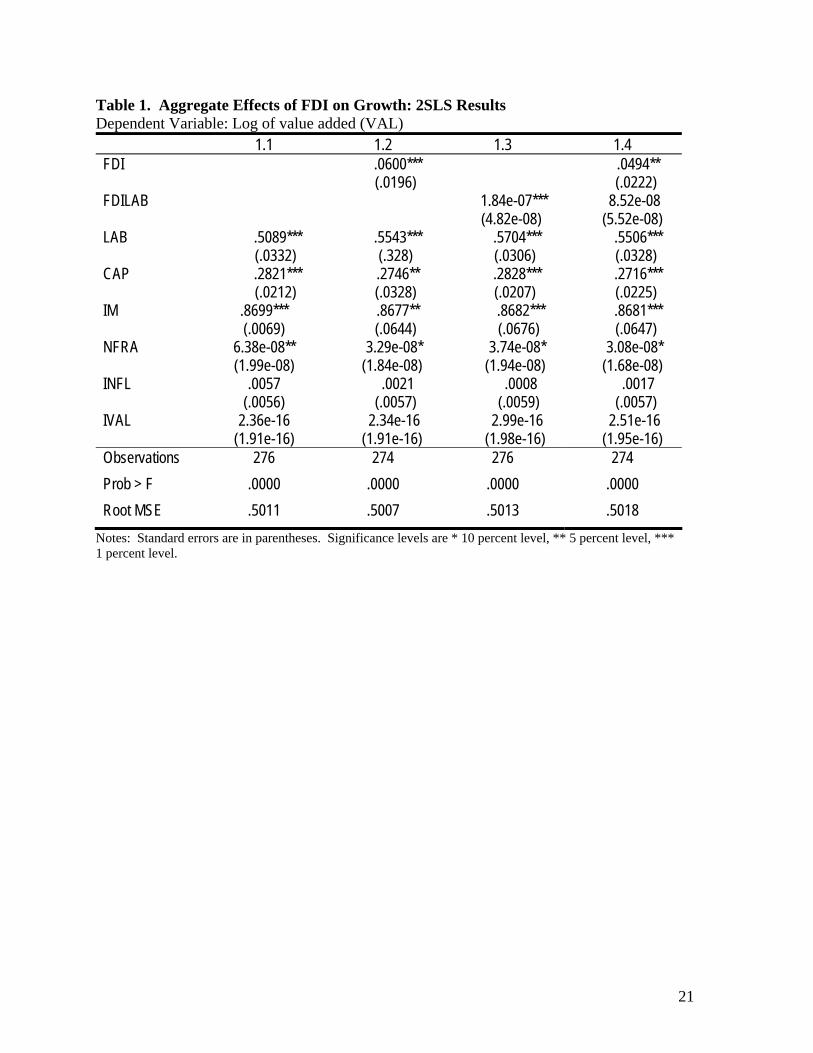
Table 1. Aggregate Effects of FDI on Growth: 2SLS Results Dependent Variable: Log of value added (VAL)

1.1 1.2 1.3 1.4 FDI .0600***

(.0196) .0494**

(.0222) FDILAB 1.84e-07***

(4.82e-08) 8.52e-08

(5.52e-08) LAB .5089***

(.0332) .5543*** (.328)

.5704*** (.0306)

.5506*** (.0328)

CAP .2821*** (.0212)

.2746** (.0328)

.2828*** (.0207)

.2716*** (.0225)

IM .8699*** (.0069)

.8677** (.0644)

.8682*** (.0676)

.8681*** (.0647)

NFRA 6.38e-08** (1.99e-08)

3.29e-08* (1.84e-08)

3.74e-08* (1.94e-08)

3.08e-08* (1.68e-08)

INFL

.0057 (.0056)

.0021 (.0057)

.0008 (.0059)

.0017 (.0057)

IVAL

2.36e-16 (1.91e-16)

2.34e-16 (1.91e-16)

2.99e-16 (1.98e-16)

2.51e-16 (1.95e-16)

Observations 276 274 276 274 Prob > F .0000 .0000 .0000 .0000 Root MSE .5011 .5007 .5013 .5018

Notes: Standard errors are in parentheses. Significance levels are * 10 percent level, ** 5 percent level, *** 1 percent level.

21

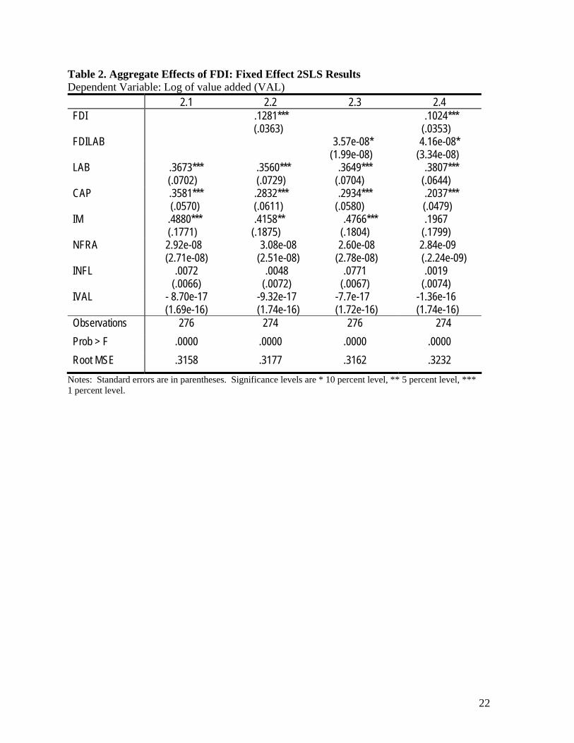
Table 2. Aggregate Effects of FDI: Fixed Effect 2SLS Results Dependent Variable: Log of value added (VAL)

2.1 2.2 2.3 2.4 FDI .1281***

(.0363) .1024***

(.0353) FDILAB 3.57e-08*

(1.99e-08) 4.16e-08*

(3.34e-08) LAB .3673***

(.0702) .3560*** (.0729)

.3649*** (.0704)

.3807*** (.0644)

CAP .3581*** (.0570)

.2832*** (.0611)

.2934*** (.0580)

.2037*** (.0479)

IM .4880*** (.1771)

.4158** (.1875)

.4766*** (.1804)

.1967 (.1799)

NFRA 2.92e-08 (2.71e-08)

3.08e-08 (2.51e-08)

2.60e-08 (2.78e-08)

2.84e-09 (.2.24e-09)

INFL

.0072 (.0066)

.0048 (.0072)

.0771 (.0067)

.0019 (.0074)

IVAL

- 8.70e-17 (1.69e-16)

-9.32e-17 (1.74e-16)

-7.7e-17 (1.72e-16)

-1.36e-16 (1.74e-16)

Observations 276 274 276 274 Prob > F .0000 .0000 .0000 .0000 Root MSE .3158 .3177 .3162 .3232

Notes: Standard errors are in parentheses. Significance levels are * 10 percent level, ** 5 percent level, *** 1 percent level.

22

Table 3. Aggregate Effects of FDI: Fixed Effect 2SLS Results for 1989-2003 Dependent Variable: Log of value added (VAL)

3.1 3.2 3.3 3.4 FDI .1036**

(.0471) .0934**

(.0472) FDILAB 3.26e-08*

(1.94e-08) 3.81e-08*

(2.24e-08) LAB .3672***

(.0815) .3475*** (.0841)

.3656*** (.0698)

.3457*** (.0828)

CAP .3583*** (.0681)

.3151*** (.0757)

.3039*** (.0817)

.3195*** (.0772)

IM .4434** (.2025)

.3843* (.2142)

.4342** (.2061)

.3738* (.2177)

NFRA 2.99e-08 (2.87e-08)

2.73e-08 (2.66e-08)

2.74e-08 (2.73e-08)

2.44e-09 (.2.68e-09)

INFL

.0045 (.0082)

.0037 (.0087)

.0045 (.0082)

.0038 (.0087)

IVAL

- 1.18e-16 (1.95e-16)

-1.17e-16 (1.99e-16)

-1.10e-16 (1.98e-16)

-1.09e-16 (2.01e-16)

Observations 216 214 216 214 Prob > F .0000 .0000 .0000 .0000 Root MSE .3272 .3250 .3232 .3258

Notes: Standard errors are in parentheses. Significance levels are * 10 percent level, ** 5 percent level, *** 1 percent level.

23

Table 4. Sectoral Effects of FDI Dependent Variable: Log of value added (VAL)

4.4 FDIxSi +FDIxLABxSi + Si + Ti + Ci Variable

4.1 FDIxSi

4.2 FDIxSi + Si +

Ti + Ci

4.3 FDIxLABxSi +

Si + Ti + Ci FDIxSi FDIxLABxSi

Real Estate .1445*** (.0405)

.3965*** (.1298)

6.81e-06*** (1.34e-06)

-1.830*** (.5012)

.00002*** (4.36e-06)

Agriculture and Fishery

-.1239*** (.0287)

-.3187*** (.1227)

-.00001* (6.19e-06)

1.915*** (.4999)

-8.63e-06 (.00002)

Mining and Quarrying

-.1176*** (.0269)

-.2541 (.1630)

-6.75e-06*** (1.55e-06)

1.965*** (.4913)

-.00002*** (4.38e-06)

Food Products

-.0929*** (.0249)

-.1748 (.1172)

-4.05e-6*** (1.15e-06)

1.581*** (.4396)

-.000015*** (3.71e-06)

Oil and Chemical

-.0883*** (.0235)

-.2668** (.1277)

-6.48e-06*** (1.31`e-06)

1.616*** (.4591)

-.000019*** (4.26e-06)

Machinery

-.0734*** (.0237)

-.3038** (.1298)

-6.29e-06*** (1.32e-06)

1.742*** (.4772)

-.000018*** (4.20e-06)

Transport Equipments

-.1157*** (.0259)

-.2089 (.1388)

-5.57e-06*** (1.28e-06)

1.748*** (.4723)

-.000018*** (4.12e-06)

Electricity Gas and Water

-.0962*** (.0208)

-.3363*** (.1303)

-5.50e-06*** (1.38e-06)

1.709*** (.4767)

-.000017*** (4.02e-06)

Construction -.0060 (.0266)

-.2424* (.1347)

6.61e-06 (2.10e-05)

1.768*** (.4561)

-9.37e-06 (5.93e-06)

Trade and Repairs

-.0328 (.0218)

-.1487 (.1243)

-6.45e-06*** (1.37e-06)

1.733*** (.4568)

-.000019*** (4.26e-06)

Hotels and Restaurants

-.0815*** (.0303)

-.3222** (.1479)

-5.51e-06*** (1.33e-06)

1.767*** (.4805)

-.000017*** (4.04e-06)

Financial Intermediation

-.0576** (.0234)

-.2819* (.1476)

-6.65e-06*** (1.38e-06)

1.302*** (.4394)

-.000019*** (4.28e-06)

Observations 274 274 274 274 Prob > F .0000 .0000 .0000 .0000 Root MSE .4622 .3311 .3504 .3934

Notes: C, S and T are country, sector, and time dummies, respectively. The coefficient reported for real estate is the slope coefficient on FDI or FDIxLAB (real estate is the omitted sectoral dummy). Standard errors are in parentheses. Significance levels are *10 percent level, **5 percent level, ***1 percent level.

24