Sections and gathers for planar re...

6.2. INTRODUCTION TO DIP 151

6.2 INTRODUCTION TO DIP

The study of seismic travel-time dependence upon source-receiver o�set begins by

calculating the travel times for rays in some ideal environments.

6.2.1 Sections and gathers for planar re ectors

The simplest environment for re ection data is a single horizontal re ection interface,

which is shown in Figure 6.12. As expected, the zero-o�set section mimics the earth

Figure 6.12: Simplest earth model. ofs-simple [NR]

model. The common-midpoint gather is a hyperbola whose asymptotes are straight

lines with slopes of the inverse of the velocity v1. The most basic data processing is

called common-depth-point stack or CDP stack. In it, all the traces on the common-

midpoint (CMP) gather are time shifted into alignment and then added together.

The result mimics a zero-o�set trace. The collection of all such traces is called the

CDP-stacked section. In practice the CDP-stacked section is often interpreted and

migrated as though it were a zero-o�set section. In this chapter we will learn to avoid

this popular, oversimpli�ed assumption.

The next simplest environment is to have a planar re ector that is oriented ver-

tically rather than horizontally. This is not typical, but is included here because

the e�ect of earth dip is more comprehensible in an extreme case. Now the wave

propagation is along the air-earth interface. To avoid confusion the re ector may be

inclined at a slight angle from the vertical, as in Figure 6.13.

Figure 6.13 shows that the travel time does not change as the o�set changes. It

may seem paradoxical that the travel time does not increase as the shot and geophone

get further apart. The key to the paradox is that midpoint is held constant, not

shotpoint. As o�set increases, the shot gets further from the re ector while the

geophone gets closer. Time lost on one path is gained on the other.

152 CHAPTER 6. OFFSET, ANOTHER DIMENSION

Figure 6.13: Near-vertical re ector, a gather, and a section. ofs-vertlay [NR]

A planar re ector may have any dip between horizontal and vertical. Then the

common-midpoint gather lies between the common-midpoint gather of Figure 6.12

and that of Figure 6.13. The zero-o�set section in Figure 6.13 is a straight line, which

turns out to be the asymptote of a family of hyperbolas. The slope of the asymptote

is the inverse of the velocity v1.

6.2.2 The dipping bed

While the travel-time curves resulting from a dipping bed are simple, they are not

simple to derive. Before the derivation, the result will be stated: for a bed dipping

at angle � from the horizontal, the travel-time curve is

t2 v2 = 4 (y � y0)2 sin2 � + 4h2 cos2 � (6:3)

For � = 45�, equation (6.3) is the familiar Pythagoras cone|it is just like t2 =

z2 + x2. For other values of �, the equation is still a cone, but a less familiar one

because of the stretched axes.

For a common-midpoint gather at y = y1 in (h; t)-space, equation (6.3) looks

like t2 = t20+ 4h2=v2apparent. Thus the common-midpoint gather contains an exact

hyperbola, regardless of the earth dip angle �. The e�ect of dip is to change the

asymptote of the hyperbola, thus changing the apparent velocity. The result has

great signi�cance in applied work and is known as Levin's dip correction [1971]:

vapparent =vearth

cos(�)(6:4)

(See also Slotnick [1959]). In summary, dip increases the stacking velocity.

Figure 6.14 depicts some rays from a common-midpoint gather. Notice that

each ray strikes the dipping bed at a di�erent place. So a common-midpoint gather is


yyo

Figure 6.14: Rays from a common-midpoint gather. ofs-dipray [NR]

not a common-depth-point gather. To realize why the re ection point moves on the

re ector, recall the basic geometrical fact that an angle bisector in a triangle generally

doesn't bisect the opposite side. The re ection point moves up dip with increasing

o�set.

Finally, equation (6.3) will be proved. Figure 6.15 shows the basic geometry along

with an \image" source on another re ector of twice the dip. For convenience,

o s yg

s ’

Figure 6.15: Travel time from image source at s0 to g may be expressed by the lawof cosines. ofs-lawcos [NR]

the bed intercepts the surface at y0 = 0. The length of the line s0g in Figure 6.15 is

determined by the trigonometric Law of Cosines to be

t2 v2 = s2 + g2 � 2 s g cos 2�

t2 v2 = (y � h)2 + (y + h)2 � 2 (y � h)(y + h) cos 2�

t2 v2 = 2 (y2 + h2) � 2 (y2�h2) (cos2 � � sin2 �)

t2 v2 = 4 y2 sin2 � + 4h2 cos2 �

which is equation (6.3).


Another facet of equation (6.3) is that it describes the constant-o�set section.

Surprisingly, the travel time of a dipping planar bed becomes curved at nonzero

o�set|it too becomes hyperbolic.

6.2.3 The point response

Another simple geometry is a re ecting point within the earth. A wave incident on the

point from any direction re ects waves in all directions. This geometry is particularly

important because any model is a superposition of such point scatterers. Figure 6.16

shows an example. The curves in Figure 6.16 include at spots for the same reasons

Figure 6.16: Response of two point scatterers. Note the at spots. ofs-twopoint [NR]

that some of the curves in �gures6.12 and 6.13 were straight lines.

The point-scatterer geometry for a point located at (x; z) is shown in Figure 6.17.

The equation for travel time t is the sum of the two travel paths

t v =qz2 + (s � x)

2+qz2 + (g � x)

2(6:5)

6.2.4 Cheops' pyramid

Because of the importance of the point-scatterer model, we will go to considerable

lengths to visualize the functional dependence among t, z, x, s, and g in equation

(6.5). This picture is more di�cult|by one dimension|than is the conic section of

the exploding-re ector geometry.

To begin with, suppose that the �rst square root in (6.5) is constant because

everything in it is held constant. This leaves the familiar hyperbola in (g; t)-space,

except that a constant has been added to the time. Suppose instead that the other


h

g

x

s

h

y

z

Figure 6.17: Geometry of a point scatterer. ofs-pgeometry [NR]

square root is constant. This likewise leaves a hyperbola in (s; t)-space. In (s; g)-

space, travel time is a function of s plus a function of g. I think of this as one coat

hanger, which is parallel to the s-axis, being hung from another coat hanger, which

is parallel to the g-axis.

A view of the travel-time pyramid on the (s; g)-plane or the (y; h)-plane is shown

in Figure 6.18a. Notice that a cut through the pyramid at large t is a square,

the corners of which have been smoothed. At very large t, a constant value of t is

the square contoured in (s; g)-space, as in Figure 6.18b. Algebraically, the squareness

becomes evident for a point re ector near the surface, say, z ! 0. Then (6.5) becomes

v t = js � xj + jg � xj (6:6)

The center of the square is located at (s; g) = (x; x). Taking travel time t to increase

downward from the horizontal plane of (s; g)-space, the square contour is like a hor-

izontal slice through the Egyptian pyramid of Cheops. To walk around the pyramid

at a constant altitude is to walk around a square. Alternately, the altitude change of

a traverse over g at constant s is simply a constant plus an absolute-value function,

as is a traverse of s at constant g.

More interesting and less obvious are the curves on common-midpoint gathers and

constant-o�set sections. Recall the de�nition that the midpoint between the shot and

geophone is y. Also recall that h is half the horizontal o�set from the shot to the

geophone.

y =g + s

2(6.7)

h =g � s

2(6.8)

A traverse of y at constant h is shown in Figure 6.18. At the highest elevation on the

traverse, you are walking along a at horizontal step like the at-topped hyperboloids


Figure 6.18: Left is a picture of the travel-time pyramid of equation ?? for �xedx and z. The darkened lines are constant-o�set sections. Right is a cross sectionthrough the pyramid for large t (or small z). (Ottolini) ofs-cheop [NR]

of Figure 6.16. Some erosion to smooth the top and edges of the pyramid gives a model

for nonzero re ector depth.

For rays that are near the vertical, the travel-time curves are far from the hyper-

bola asymptotes. Then the square roots in (6.5) may be expanded in Taylor series,

giving a parabola of revolution. This describes the eroded peak of the pyramid.

6.2.5 Random point scatterers

Figure 6.19 shows a synthetic constant-o�set section (COS) taken from an earth

model containing about �fty randomly placed point scatterers. Late arrival times

Figure 6.19: Constant-o�set section over random point scatterers. ofs-randcos [NR]


appear hyperbolic. Earlier arrivals have attened tops. The earliest possible arrival

corresponds to a ray going horizontally from the shot to the geophone.

Figure 6.20 shows a synthetic common-shot pro�le (CSP) from the same earth

model of random point scatterers. Each scatterer produces a hyperbolic arrival.

Figure 6.20: Common-shot pro-�le over random point scatterers.ofs-randcsp [NR]

The hyperbolas are not symmetric around zero o�set; their locations are random.

They must, however, all lie under the lines jg� sj = vt. Hyperbolas with sharp tops

can be found at late times as well as early times. However, the sharp tops, which are

from shallow scatterers near the geophone, must lie near the lines jg � sj = vt.

The left side of Figure 6.21 shows a synthetic common-midpoint gather (CMP)

from an earth model containing about �fty randomly placed point scatterers.

Figure 6.21: Common-midpoint gather on earth of randomly located point scatterers(left). The same gathers after NMO correction (right). ofs-randcmp [NR]

Because this is a common-midpoint gather, the curves are symmetric through zero

o�set. (The negative o�sets of �eld data are hardly ever plotted). Some of the


arrivals have attened tops, which indicate scatterers that are not directly under the

midpoint.

Normal-moveout (NMO) correction is a stretching of the data to try to atten the

hyperbolas. This correction assumes at beds, but it also works for point scatterers

that are directly under the midpoint. The right side of Figure 6.21 shows what

happens when normal-moveout correction is applied on the random scatterer model.

Some re ectors are attened; others are \overcorrected."

6.2.6 Forward and backward scattering: Larner's streaks

At some locations, near-surface waves overwhelm the deep re ections of geologic

interest. Compounding our di�culty, the near-surface waves are usually irregular

because the earth is comparatively more irregular at its surface than deeper down.

On land, these interfering waves are called ground roll. At sea, they are called water

waves (not to be confused with surface waves on water).

A model for such near-surface noises is suggested by the vertical re ecting wall in

Figure 6.13. In this model the waves remain close to the surface. Randomly placed

vertical walls could result in a zero-o�set section that resembles the �eld data of

Figure 6.22. Another less extreme model for the surface noises is the at-topped

curves in the random point-scatterer model.

Figure 6.22: CDP stack with water noise from the Shelikof Strait, Alaska. (by per-mission from Geophysics, Larner et al. [1983]) ofs-shelikof [NR]

In the random point-re ector model the velocity was a constant. In real life the

earth velocity is generally slower for the near-surface waves and faster for the deep

re ections. This sets the stage for some unexpected noise ampli�cation.


CDP stacking enhances events with the stacking velocity and discriminates against

events with other velocities. Thus you might expect that stacking at deeper, higher

velocity would discriminate against low-velocity, near-surface events. Near-surface

noises, however, are not re ections from horizontal layers; they are more like re ec-

tions from vertical walls or steeply dipping layers. But equation (6.4) shows that dip

increases the apparent velocity. So it is not surprising that stacking at deep-sediment,

high velocities can enhance surface noises. Occurrence of this problem in practice was

nicely explained and illustrated by Larner et al. [1983]

6.2.7 Velocity of sideswipe

Shallow-water noise can come from waves scattering from a sunken ship or from

the side of an island or iceberg several kilometers to the side of the survey line.

Think of boulders strewn all over a shallow sea oor, not only along the path of

the ship, but also o� to the sides. (Reality is more impressive. Wind blown ice

ows drag themselves along the bottom making huge scars in it.) The travel-time

curves for re ections from the boulders nicely matches the random point-scatterer

model. Because of the long wavelengths of seismic waves, our sending and receiving

equipment does not enable us to distinguish waves going up and down from those

going sideways.

Imagine one of these shallow scatterers several kilometers to the side of the ship.

More precisely, let the scatterer be on the earth's surface, perpendicular to the mid-

point of the line connecting the shot point to the geophone. A common-midpoint

gather for this scatterer is a perfect hyperbola, as from the deep re ector contribu-

tions on Figure 6.20. Since it is a water-velocity hyperbola, this scatterered noise

should be nicely suppressed by CDP stacking with the higher, sediment velocity. So

the \streaking" scatterers in Figure 6.22 are not sidescatter.

The \streaking" scatterers are those neither along the survey line nor those per-

pendicular to it. The \in-line" scatterers have in�nite velocity (on the at spot). The

scatterers perpendicular to the survey line have the water velocity. Scatterers at other

angles have inbetween velocities and they stack strongly at the sediment velocity and

account for the streaks.

6.2.8 The migration ellipse

Another insight into equation (6.5) is to regard the o�set h and the total travel time

t as �xed constants. Then the locus of possible re ectors turns out to describe an

ellipse in the plane of (y�y0; z). The reason it is an ellipse follows from the geometric

de�nition of an ellipse. To draw an ellipse, place a nail or tack into s on Figure 6.17

and another into g. Connect the tacks by a string that is exactly long enough to

go through (y0; z). An ellipse going through (y0; z) may be constructed by sliding a

pencil along the string, keeping the string tight. The string keeps the total distance

tv constant.


Recall that one method for migrating zero-o�set sections is to take every data

value in (y; t)-space and use it to superpose an appropriate semicircle in (y; z)-space.

For nonzero o�set the circle should be generalized to an ellipse (Figure 3.6).

It is not easy to show that equation (6.5) can be cast in the standard mathematical

form of an ellipse, namely, a stretched circle. But the result is a simple one, and an

important one for later analysis, so here we go. Equation (6.5) in (y; h)-space is

t v =qz2 + (y � y0 � h)

2+qz2 + (y � y0 + h)

2(6:9)

To help reduce algebraic verbosity, de�ne a new y equal to the old one shifted by y0.

Also make the de�nitions

t vrock = 2 d = 2 t vhalf (6.10)

a = z2 + (y + h)2 (6.11)

b = z2 + (y � h)2 (6.12)

a � b = 4 y h (6.13)

With these de�nitions, (6.9) becomes

2 d =pa +

pb (6:14)

Square to get a new equation with only one square root.

4 d2 � (a + b) = 2papb (6:15)

Square again to eliminate the square root.

16 d4 � 8 d2 (a + b) + (a + b)2 = 4 a b (6.16)

16 d4 � 8 d2 (a + b) + (a � b)2 = 0 (6.17)

Introduce de�nitions of a and b.

16 d4 � 8 d2 [ 2 z2 + 2 y2 + 2h2] + 16 y2 h2 = 0 (6:18)

Bring y and z to the right.

d4 � d2 h2 = d2 (z2 + y2) � y2 h2 (6.19)

d2 (d2 � h2) = d2 z2 + (d2 � h2) y2 (6.20)

d2 =z2

1 � h2

d2

+ y2 (6.21)

Finally, recalling all earlier de�nitions,

t2 v2half =z2

1 � h2

t2 v2half

+ (y � y0)2 (6:22)

Fixing t, equation (6.22) is the equation for a circle with a stretched z-axis. Our

algebra has con�rmed that the \string and tack" de�nition of an ellipse matches the

\stretched circle" de�nition. An ellipse in model space is the earth model given the

observation of an impulse on a constant-o�set section.

6.3. SURVEY SINKING WITH THE DOUBLE-SQUARE-ROOT EQUATION 161

h hy

z

yo

Figure 6.23: Migration ellipse. ofs-ellipse [NR]

6.3 SURVEY SINKINGWITH THE DOUBLE-SQUARE-

ROOT EQUATION

Exploding-re ector imaging will be replaced by a broader imaging concept, survey

sinking. A new equation called the double-square-root (DSR) equation will be de-

veloped to implement survey-sinking imaging. The function of the DSR equation

is to downward continue an entire seismic survey, not just the geophones but also

the shots. After deriving the DSR equation, the remainder of this chapter will be

devoted to explaining migration, stacking, migration before stack, velocity analysis,

and corrections for lateral velocity variations in terms of the DSR equation.

Peek ahead at equation (6.35) and you will see an equation with two square roots.

One represents the cosine of the wave arrival angle. The other represents the takeo�

angle at the shot. One cosine is expressed in terms of kg, the Fourier component

along the geophone axis of the data volume in (s; g; t)-space. The other cosine, with

ks, is the Fourier component along the shot axis.

Our �eld seismograms lie in the (s; g)-plane. To move onto the (y; h)-plane in-

habited by seismic interpreters requires only a simple rotation. The data could be

Fourier transformed with respect to y and h, for example. Then downward continu-

ation would proceed with equation (6.48) instead of equation (6.35).

The DSR equation depends upon the reciprocity principle which we will review

�rst.


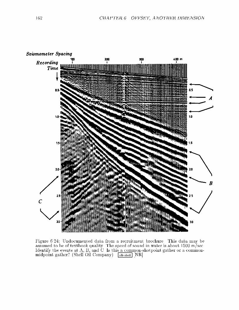
Figure 6.24: Undocumented data from a recruitment brochure. This data may beassumed to be of textbook quality. The speed of sound in water is about 1500 m/sec.Identify the events at A, B, and C. Is this a common-shotpoint gather or a common-midpoint gather? (Shell Oil Company) ofs-shell [NR]


6.3.1 Seismic reciprocity in principle and in practice

The principle of reciprocity says that the same seismogram should be recorded if

the locations of the source and geophone are exchanged. A physical reason for the

validity of reciprocity is that no matter how complicated a geometrical arrangement,

the speed of sound along a ray is the same in either direction.

Mathematically, the reciprocity principle arises because the physical equations

of elasticity are self adjoint. The meaning of the term self adjoint is illustrated in

FGDP where it is shown that discretized acoustic equations yield a symmetric matrix

even where density and compressibility are space variable. The inverse of any such

symmetric matrix is another symmetric matrix called the impulse-response matrix.

Elements across the matrix diagonal are equal to one another. Each element of any

pair is a response to an impulsive source. The opposite element of the pair refers to

the interchanged source and receiver.

A tricky thing about the reciprocity principle is the way antenna patterns must be

handled. For example, a single vertical geophone has a natural antenna pattern. It

cannot see horizontally propagating pressure waves nor vertically propagating shear

waves. For reciprocity to be applicable, antenna patterns must not be interchanged

when source and receiver are interchanged. The antenna pattern must be regarded

as attached to the medium.

I searched our data library for split-spread land data that would illustrate reci-

procity under �eld conditions. The constant-o�set section in Figure 6.25 was recorded

by vertical vibrators into vertical geophones. The survey was not intended to be a

test of reciprocity, so there likely was a slight lateral o�set of the source line from the

receiver line. Likewise the sender and receiver arrays (clusters) may have a slightly

di�erent geometry. The earth dips in Figure 6.25 happen to be quite small although

lateral velocity variation is known to be a problem in this area.

In Figure 6.26, three seismograms were plotted on top of their reciprocals. Pairs

were chosen at near o�set, at mid range, and at far o�set. You can see that reciprocal

seismograms usually have the same polarity, and often have nearly equal amplitudes.

(The �gure shown is the best of three such �gures I prepared).

Each constant time slice in Figure 6.27 shows the reciprocity of many seismogram

pairs. Midpoint runs horizontally over the same range as in Figure 6.25. O�set

is vertical. Data is not recorded near the vibrators leaving a gap in the middle.

To minimize irrelevant variations, moveout correction was done before making the

time slices. (There is a missing source that shows up on the left side of the �gure).

A movie of panels like Figure 6.27 shows that the bilateral symmetry you see in

the individual panels is characteristic of all times. Notice however that there is a

signi�cant departure from reciprocity on the one-second time slice around midpoint

120.

In the laboratory, reciprocity can be established to within the accuracy of mea-

surement. This can be excellent. (See White's example in FGDP). In the �eld,

the validity of reciprocity will be dependent on the degree that the required con-


Figure 6.25: Constant-o�set section from the Central Valley of California. (Chevron)ofs-toldi [ER]

Figure 6.26: Overlain reciprocal seismograms. ofs-reciptrace [ER]


Figure 6.27: Constant time slices after NMO at 1 second and 2.5 seconds. ofs-recipslice

[ER]

ditions are ful�lled. A marine air gun should be reciprocal to a hydrophone. A

land-surface weight-drop source should be reciprocal to a vertical geophone. But a

buried explosive shot need not be reciprocal to a surface vertical geophone because

the radiation patterns are di�erent and the positions are slightly di�erent. Fenati and

Rocca [1984] studied reciprocity under varying �eld conditions. They reported that

small positioning errors in the placement of sources and receivers can easily create dis-

crepancies larger than the apparent reciprocity discrepancy. They also reported that

theoretically reciprocal experiments may actually be less reciprocal than presumably

nonreciprocal experiments.

Geometrical complexity within the earth does not diminish the applicability of

the principle of linearity. Likewise, geometrical complexity does not reduce the appli-

cability of reciprocity. Reciprocity does not apply to sound waves in the presence of

wind. Sound goes slower upwind than downwind. But this e�ect of wind is much less

than the mundane irregularities of �eld work. Just the weakening of echoes with time

leaves noises that are not reciprocal. Henceforth we will presume that reciprocity is

generally applicable to the analysis of re ection seismic data.

6.3.2 The survey-sinking concept

The exploding-re ector concept has great utility because it enables us to associate

the seismic waves observed at zero o�set in many experiments (say 1000 shot points)

with the wave of a single thought experiment, the exploding-re ector experiment.

The exploding-re ector analogy has a few tolerable limitations connected with lateral

velocity variations and multiple re ections, and one major limitation: it gives us no

clue as to how to migrate data recorded at nonzero o�set. A broader imaging concept

is needed.


Start from �eld data where a survey line has been run along the x-axis. Assume

there has been an in�nite number of experiments, a single experiment consisting of

placing a point source or shot at s on the x-axis and recording echoes with geophones

at each possible location g on the x-axis. So the observed data is an upcoming wave

that is a two-dimensional function of s and g, say P (s; g; t).

Previous chapters have shown how to downward continue the upcoming wave.

Downward continuation of the upcoming wave is really the same thing as downward

continuation of the geophones. It is irrelevant for the continuation procedures where

the wave originates. It could begin from an exploding re ector, or it could begin at

the surface, go down, and then be re ected back upward.

To apply the imaging concept of survey sinking, it is necessary to downward

continue the sources as well as the geophones. We already know how to downward

continue geophones. Since reciprocity permits interchanging geophones with shots,

we really know how to downward continue shots too.

Shots and geophones may be downward continued to di�erent levels, and they

may be at di�erent levels during the process, but for the �nal result they are only

required to be at the same level. That is, taking zs to be the depth of the shots and

zg to be the depth of the geophones, the downward-continued survey will be required

at all levels z = zs = zg.

The image of a re ector at (x; z) is de�ned to be the strength and polarity of

the echo seen by the closest possible source-geophone pair. Taking the mathematical

limit, this closest pair is a source and geophone located together on the re ector. The

travel time for the echo is zero. This survey-sinking concept of imaging is summarized

by

Image(x; z) = Wave(s = x; g = x; z; t = 0) (6:23)

For good quality data, i.e. data that �ts the assumptions of the downward-continuation

method, energy should migrate to zero o�set at zero travel time. Study of the energy

that doesn't do so should enable improvement of the model. Model improvement

usually amounts to improving the spatial distribution of velocity.

6.3.3 Review of the paraxial wave equation

An equation was derived for paraxial waves. The assumption of a single plane wave

means that the arrival time of the wave is given by a single-valued t(x; z). On a plane

of constant z, such as the earth's surface, Snell's parameter p is measurable. It is

@t

@x=

sin �

v= p (6:24)

In a borehole there is the constraint that measurements must be made at a constant

x, where the relevant measurement from an upcoming wave would be

@t

@z= � cos �

v= �

vuut 1

v2� @t

@x

!2

(6:25)


Recall the time-shifting partial-di�erential equation and its solution U as some arbi-

trary functional form f :

@U

@z= � @t

@z

@U

@t(6.26)

U = f

t �

Z z

0

@t

@zdz

!(6.27)

The partial derivatives in equation (6.26) are taken to be at constant x, just as is

equation (6.25). After inserting (6.25) into (6.26) we have

@U

@z=

vuut 1

v2� @t

@x

!2@U

@t(6:28)

Fourier transforming the wave�eld over (x; t), we replace @=@t by � i!. Likewise, for

the traveling wave of the Fourier kernel exp(� i!t + ikxx), constant phase means

that @t=@x = kx=!. With this, (6.28) becomes

@U

@z= � i!

s1

v2� k2x

!2U (6:29)

The solutions to (6.29) agree with those to the scalar wave equation unless v is

a function of z, in which case the scalar wave equation has both upcoming and

downgoing solutions, whereas (6.29) has only upcoming solutions. Chapter 4 taught

us how to go into the lateral space domain by replacing ikx by @=@x. The resulting

equation is useful for superpositions of many local plane waves and for lateral velocity

variations v(x).

6.3.4 The DSR equation in shot-geophone space

Let the geophones descend a distance dzg into the earth. The change of the travel

time of the observed upcoming wave will be

@t

@zg= �

vuut 1

v2� @t

@g

!2

(6:30)

Suppose the shots had been let o� at depth dzs instead of at z = 0. Likewise then,

@t

@zs= �

vuut 1

v2� @t

@s

!2

(6:31)

Both (6.30) and (6.31) require minus signs because the travel time decreases as either

geophones or shots move down.


Simultaneously downward project both the shots and geophones by an identical

vertical amount dz = dzg = dzs. The travel-time change is the sum of (6.30) and

(6.31), namely,

dt =@t

@zgdzg +

@t

@zsdzs =

@t

@zg+

@t

@zs

!dz (6:32)

or

@t

@z= �

0B@vuut 1

v2� @t

@g

!2

+

vuut 1

v2�

@t

@s

!21CA (6:33)

This expression for @t=@z may be substituted into equation (6.26):

@U

@z= +

0B@vuut 1

v2�

@t

@g

!2

+

vuut 1

v2� @t

@s

!21CA @U

@t(6:34)

Three-dimensional Fourier transformation converts upcoming wave data u(t; s; g)

to U(!; ks; kg). Expressing equation (6.34) in Fourier space gives

@U

@z= � i !

264vuut 1

v2�

kg

!

!2

+

vuut 1

v2� ks

!

!2375 U (6:35)

Recall the origin of the two square roots in equation (6.35). One is the cosine of the

arrival angle at the geophones divided by the velocity at the geophones. The other is

the cosine of the takeo� angle at the shots divided by the velocity at the shots. With

the wisdom of previous chapters we know how to go into the lateral space domain

by replacing ikg by @=@g and iks by @=@s. To incorporate lateral velocity variation

v(x), the velocity at the shot location must be distinguished from the velocity at the

geophone location. Thus,

@U

@z=

264vuut � � i!

v(g)

�2

� @2

@g2+

s �� i!

v(s)

�2

� @2

@s2

375 U (6:36)

Equation (6.36) is known as the double-square-root (DSR) equation in shot-

geophone space. It might be more descriptive to call it the survey-sinking equation

since it pushes geophones and shots downward together. Recalling the section on

splitting and full separation we realize that the two square-root operators are com-

mutative (v(s) commutes with @=@g), so it is completely equivalent to downward

continue shots and geophones separately or together. This equation will produce

waves for the rays that are found on zero-o�set sections but are absent from the

exploding-re ector model.


6.3.5 The DSR equation in midpoint-o�set space

By converting the DSR equation to midpoint-o�set space we will be able to identify

the familiar zero-o�set migration part along with corrections for o�set. The trans-

formation between (g; s) recording parameters and (y; h) interpretation parameters

is

y =g + s

2(6.37)

h =g � s

2(6.38)

Travel time t may be parameterized in (g; s)-space or (y; h)-space. Di�erential rela-

tions for this conversion are given by the chain rule for derivatives:

@t

@g=

@t

@y

@y

@g+

@t

@h

@h

@g=

1

2

@t

@y+

@t

@h

!(6.39)

@t

@s=

@t

@y

@y

@s+

@t

@h

@h

@s=

1

2

@t

@y� @t

@h

!(6.40)

Having seen how stepouts transform from shot-geophone space to midpoint-o�set

space, let us next see that spatial frequencies transform in much the same way.

Clearly, data could be transformed from (s; g)-space to (y; h)-space with (6.37) and

(6.38) and then Fourier transformed to (ky; kh)-space. The question is then, what form

would the double-square-root equation (6.35) take in terms of the spatial frequencies

(ky; kh)? De�ne the seismic data �eld in either coordinate system as

U(s; g) = U 0(y; h) (6:41)

This introduces a new mathematical function U 0 with the same physical meaning as

U but, like a computer subroutine or function call, with a di�erent subscript look-up

procedure for (y; h) than for (s; g). Applying the chain rule for partial di�erentiation

to (6.41) gives

@U

@s=

@y

@s

@U 0

@y+

@h

@s

@U 0

@h(6.42)

@U

@g=

@y

@g

@U 0

@y+

@h

@g

@U 0

@h(6.43)

and utilizing (6.37) and (6.38) gives

@U

@s=

1

2

@U 0

@y� @U 0

@h

!(6.44)

@U

@g=

1

2

@U 0

@y+

@U 0

@h

!(6.45)


In Fourier transform space where @=@x transforms to ikx, equations (6.44) and (6.45),

when i and U = U 0 are cancelled, become

ks =1

2(ky � kh) (6.46)

kg =1

2(ky + kh) (6.47)

Equations (6.46) and (6.47) are Fourier representations of (6.44) and (6.45). Substi-

tuting (6.46) and (6.47) into (6.35) achieves the main purpose of this section, which

is to get the double-square-root migration equation into midpoint-o�set coordinates:

@

@zU = � i

!

v

264vuut 1 �

vky + vkh

2!

!2

+

vuut 1 � vky � vkh

2!

!2375 U (6:48)

Equation (6.48) is the takeo� point for many kinds of common-midpoint seismo-

gram analyses. Some convenient de�nitions that simplify its appearance are

G =v kg

!(6.49)

S =v ks

!(6.50)

Y =v ky

2 !(6.51)

H =v kh

2 !(6.52)

Chapter 3 showed that the quantity v kx=! can be interpreted as the angle of a wave.

Thus the new de�nitions S and G are the sines of the takeo� angle and of the arrival

angle of a ray. When these sines are at their limits of �1 they refer to the steepest

possible slopes in (s; t)- or (g; t)-space. Likewise, Y may be interpreted as the dip

of the data as seen on a seismic section. The quantity H refers to stepout observed

on a common-midpoint gather. With these de�nitions (6.48) becomes slightly less

cluttered:

@

@zU = � i!

v

�q1� (Y +H)2 +

q1� (Y �H)2

�U (6:53)

Most present-day before-stack migration procedures can be interpreted through

equation (6.53). Further analysis of it will explain the limitations of conventional

processing procedures as well as suggest improvements in the procedures.

EXERCISES:

1 Adapt equation (6.48) to allow for a di�erence in velocity between the shot and

the geophone.

6.4. THE MEANING OF THE DSR EQUATION 171

2 Adapt equation (6.48) to allow for downgoing pressure waves and upcoming shear

waves.

6.4 THE MEANING OF THE DSR EQUATION

The double-square-root equation contains most nonstatistical aspects of seismic data

processing for petroleum prospecting. This equation, which was derived in the previ-

ous section, is not easy to understand because it is an operator in a four-dimensional

space, namely, (z; s; g; t). We will approach it through various applications, each of

which is like a picture in a space of lower dimension. In this section lateral velocity

variation will be neglected (things are bad enough already!). Begin with

dU

dz=

� i!

v

� p1 � G2 +

p1 � S2

�U (6.54)

dU

dz=

� i!

v

� q1 � (Y +H)2 +

q1 � (Y �H)2

�U (6.55)

6.4.1 Zero-o�set migration (H = 0)

One way to reduce the dimensionality of (6.55) is simply to set H = 0. Then the

two square roots become the same, so that they can be combined to give the familiar

paraxial equation:

dU

dz= � i!

2

v

s1 �

v2 k2y

4!2U (6:56)

In both places in equation (6.56) where the rock velocity occurs, the rock velocity

is divided by 2. Recall that the rock velocity needed to be halved in order for �eld

data to correspond to the exploding-re ector model. So whatever we did by setting

H = 0, gave us the same migration equation we used in chapter 3. Setting H = 0

had the e�ect of making the survey-sinking concept functionally equivalent to the

exploding-re ector concept.

6.4.2 Zero-dip stacking (Y = 0)

When dealing with the o�set h it is common to assume that the earth is horizontally

layered so that experimental results will be independent of the midpoint y. With such

an earth the Fourier transform of all data over y will vanish except for ky = 0, or,

in other words, for Y = 0. The two square roots in (6.54) and (6.55) again become

identical, and the resulting equation is once more the paraxial equation:

dU

dz= � i!

2

v

s1 � v2 k2h

4!2U (6:57)


Figure 6.28: With an earth model of three layers, the common-midpoint gathersare three hyperboloids. Successive frames show downward continuation to successivedepths where best focus occurs. ofs-dc2 [NR]

Using this equation to downward continue hyperboloids from the earth's surface, we

�nd the hyperboloids shrinking with depth, until the correct depth where best focus

occurs is reached. This is shown in Figure 6.28.

The waves focus best at zero o�set. The focus represents a downward-continued

experiment, in which the downward continuation has gone just to a re ector. The

re ection is strongest at zero travel time for a coincident source-receiver pair just

above the re ector. Extracting the zero-o�set value at t = 0 and abandoning the

other o�sets is a way of eliminating noise. (Actually it is a way of de�ning noise).

Roughly it amounts to the same thing as the conventional procedure of summation

along a hyperbolic trajectory on the original data. Naturally the summation can be

expected to be best when the velocity used for downward continuation comes closest

to the velocity of the earth. Later, o�set space will be used to determine velocity.

6.4.3 Conventional processing|separable approximation

The DSR operator is now de�ned as the parenthesized operator in equation (1b):

DSR(Y;H) =q1 � (Y �H)2 +

q1 � (Y +H)2 (6:58)

In Fourier space, downward continuation is done with the operator exp(i!v�1 DSR z).

There is a serious problem with this operator: it is not separable into a sum of an


o�set operator and a midpoint operator. Nonseparable means that a Taylor series for

(6.58) contains terms like Y 2H2. Such terms cannot be expressed as a function of Y

plus a function of H. Nonseparability is a data-processing disaster. It implies that

migration and stacking must be done simultaneously, not sequentially. The only way

to recover pure separability would be to return to the space of S and G. (That is a

drastic alternative, far from conventional processing. We will return to it later).

Let us review the general issue of separability. The obvious way to get a separable

approximation of the operatorp1 � X2 � Y 2 is to form a Taylor series expansion,

and then drop all the cross terms. A more clever approximation isp1 � X2 +p

1 � Y 2 � 1, which �ts all Y exactly when X = 0 and all X exactly when Y = 0.

Applying this idea (though not the same equation) to the DSR operator gives

SEP(Y;H) = 2 + [DSR(Y; 0) � 2] + [DSR(0; H) � 2] (6.59)

SEP(Y;H) = 2 [1 + (p1 � Y 2 � 1) + (

p1 � H2 � 1)] (6.60)

Notice that at H = 0 (6.59) and (6.60) become equal to the DSR operator. At Y = 0

(6.59) and (6.60) also become equal to the DSR operator. Only when both H and Y

are nonzero does SEP depart from DSR.

The splitting of (6.59) and (6.60) into a sum of three operators o�ers an advantage

like the one o�ered by the 2-D Fourier kernel exp(ikyy + ikhh), which has a phase

that is the sum of two parts. It means that Fourier integrals may have either y or h

nested on the inside. So downward continuation with SEP could be done in (kh; ky)-

space as implied by (6.55), or we could choose to Fourier transform to (h; ky), (kh; y),

or (y; h) by appropriate nesting operations.

It is convenient to give familiar names to the three terms in (6.60). The �rst is

associated with time-to-depth conversion, the second with migration, and the third

with normal moveout.

SEP(Y;H) = TD + MIG(Y ) + NMO(H) (6:61)

The approximation (6.59) and (6.60) can be interpreted as \standard processing."

The �rst stage in standard processing is NMO correction. In (6.59) and (6.60) the

NMO operator downward continues all o�sets at the earth's surface, to all o�sets at

depth. Selecting zero o�set is no more than abandoning all other o�sets. Like stacking

over o�set, selecting zero o�set reduces the amount of data under consideration.

Ordinarily the abandoned o�sets are not migrated. (Alternately, a clever proce-

dure for changing stacking velocities after migration involves migrating several o�sets

near zero o�set).

Since all terms in the SEP operator are interchangeable, it would seem wasteful

to use it to migrate all o�sets before stack. The result of doing so should be identical

to after-stack migration.


6.4.4 Various meanings of H = 0

Recall the various forms of the stepout operator:

Forms of stepout operator 2H=v

ray trace Fourier PDE

dt

dh

kh

!@th =

tR�1

dt@

@h

Reciprocity suggests that travel time is a symmetrical function of o�set; thus

dt=dh vanishes at h = 0. In that sense it seems appropriate to apply equation (6.56)

to zero-o�set sections. More precisely, the ray-trace expression dt=dh strictly applies

only when a single plane wave is present. Spherical wavefronts are made from the

superposition of plane waves. Then the Fourier interpretation ofH is slightly di�erent

and more appropriate. To set ! = 0 would be to select a zero frequency component,

a simple integral of a seismic trace. To set kh = 0 would be to select a zero spatial-

frequency component, that is, an integration over o�set. Conventional stacking may

be de�ned as integration (or summation) over o�set along a hyperbolic trajectory.

Simply setting kh = 0 is selecting a hyperbolic trajectory that is at, namely, the

hyperbola of in�nite velocity. Such an integration will receive its major contribution

from the top of the data hyperboloid, where the data events come tangent to the

horizontal line of integration. (For some historical reason, such a data summation

is often called vertical stack). Of the total contribution to the integral, most comes

from a zone near the top, before the stepout equals a half-wavelength. The width

of this zone, which is called a Fresnel zone, is the major factor contributing to the

integral. The Fresnel zone has been extracted from a �eld pro�le in Figure 6.29.

The de�nition of the Fresnel zone involves a frequency. For practical purposes

we may just look at zero crossings. Examining Figure 6.29 near one second we see

a variety of frequencies. In the interval between t = 1:0 and t = 1:1 I see about

two wavelengths of low frequencies and about 5 wavelengths of high frequencies. The

highest frequencies are the main concern, because they de�ne the limit of seismic

resolution. The higher frequency has about 100 half wavelengths between time zero

and a time of one second. As a rough generality, this observed value of 100 applies to

all travel times. That is, at any travel time, the highest frequency that has meaningful

spatial correlations is often observed to have a half period of about 1/100 of the total

travel time. We may say that the quality factor Q of the earth's sedimentary crust is

often about 100. So the angle that we are typically thinking about is cos 8� = :99.

Theoretically, the main di�erences between a zero-o�set section and a vertical

stack are the amplitude and a small phase shift. In practical cases they are unlikely


Figure 6.29: (left) A land pro�le from Denmark (Western Geophysical) with theFresnel zone extracted and redisplayed (right). ofs-denmark [ER]


to migrate in a signi�cantly di�erent way. It would be nice if we could �nd an equation

to downward continue data that is stacked at velocities other than in�nite velocity.

The partial-di�erential-equation point of view of setting H = 0 is identical with

the Fourier view when the velocity is a constant function of the horizontal coordinate;

but otherwise the PDE viewpoint is a slightly more general one. To be speci�c, but

not cluttered, equations (6.54) and(6.55) can be expressed in 15� retarded, space-

domain form. Thus,"@

@z+

v

� i! 8

@2

@y2+

@2

@h2

! #U 0 = 0 (6:62)

Integrate this equation over o�set h. The integral commutes with the di�erential op-

erators. Recall that the integral of a derivative is the di�erence between the function

evaluated at the upper limit and the function evaluated at the lower limit. Thus,

@

@z+

v

� i! 8

@2

@y

2 !�ZU dh

�+

v

� i! 8

@U

@h

��h = +1

h = �1= 0 (6:63)

The wave should vanish at in�nite o�set and so should its horizontal o�set derivative.

Thus the last term in (6.63) should vanish. So, setting H = 0 has the meaning

(Paraxial operator (vertical stack = 0 (6:64)

A problem in the development of (6.64) was that, twice, it was assumed that ve-

locity is independent of o�set: �rst, when the thin-lens term was omitted from (6.62),

and second, when the o�set integration operator was interchanged with multiplication

by velocity. If the velocity depends on the horizontal x-axis, then it certainly depends

on both midpoint and o�set. In conclusion: If velocity changes slowly across a Fres-

nel zone, then setting H = 0 provides a valid equation for downward continuation of

vertically stacked data.

6.4.5 Clayton's cosine corrections

A tendency exists to associate the sine of the earth dip angle with Y and the sine

of the shot-geophone o�set angle with H. While this is roughly valid, there is an

important correction. Consider the dipping bed shown in Figure 6.30.

The dip angle of the re ector is �, and the o�set is expressed as the o�set angle

�. Clayton showed, and it will be veri�ed, that

Y = sin � cos � (6.65)

H = sin � cos � (6.66)

For small positive or negative angles the cosines can be ignored, and it is then

correct to associate the sine of the earth dip angle with Y and the sine of the o�set


Figure 6.30: Geometry of a dip-ping bed. The line bisecting theangle 2� does not pass throughthe midpoint between g and s.(Clayton) ofs-clay [NR]

sg

angle with H. At moderate angles the cosine correction is required. At angles ex-

ceeding 45� the sensitivities reverse, and conventional wisdom is exactly opposite to

the truth. The reader should be wary of informal discussions that simply associate

Y with dip and H with velocity. \Larner's streaks" were an example of mixing the

e�ects of dip and o�set. Indeed, at steep dips the usual procedure of using H to

determine velocity should be changed somehow to use Y .

Next, (6.65) and (6.66) will be proven. The source takeo� angle is s, and the

incident receiver angle is g. First, relate s and g to � and �. Adding up the angles

of the smaller constructed triangle gives

(�

2� s � �) + � +

�

2= �

s = � � � (6.67)

Adding up the angles around the larger triangle gives

g = � + � (6:68)

To associate the angles at depth, � and �, with the stepouts dt=ds and dt=dg at the

earth's surface requires taking care with the signs, noting that travel time increases

as the geophone moves right and decreases as the shot moves right. Recall from

equations (6.46), (6.47), (6.49), (6.50), (6.51) and (6.52), the de�nitions of apparent

angles Y and H,

Y � H = S =v ks

!= v

dt

ds= � sin s = sin(� � �) (6.69)

Y + H = G =v kg

!= v

dt

dg= + sin g = sin(� + �) (6.70)

Adding and subtracting this pair of equations and using the angle sum formula from

trigonometry gives Clayton's cosine corrections (8):

Y =1

2sin(� + �) +

1

2sin(� � �) = sin � cos � (6.71)

H =1

2sin(� + �) � 1

2sin(� � �) = sin � cos � (6.72)


6.4.6 Snell-wave stacks and CMP slant stacks

Setting the takeo� angle S to zero also reduces the double-square-root equation to

a single-square-root equation. The meaning of S = 0 is that ks = 0 or equivalently

that the data should undergo a summation (without time shifting) over shot s. Such

a summation simulates a downgoing plane wave. The imaging principle behind the

summation would be to look at the upcoming wave at the arrival time of the down-

going wave. S could also be set equal a constant, to simulate a downgoing Snell

wave.

A Snell wave is a generalization of a downgoing plane wave at nonvertical inci-

dence. The shots are not �red simultaneously, but sequentially at an inverse rate of

dt=ds = S=v. This could be simulated with �eld data by summing across the (t; s)-

plane along a line of slope dt=ds. Setting S to be some constant, say S = v dt=ds,

also reduces the double-square-root equation to a paraxial wave equation, just the

equation needed to downward continue the downgoing Snell wave experiment. Snell

waves could be constructed for various p = dt=ds values. Each could be migrated and

imaged, and the images stacked over p. These ideas have been around longer than

the DSR equation, yet they have gained no popularity. What could be the reason?

A problem with Snell wave simulation is that the wave�eld is usually sampled at

coarse intervals along a geophone cable, which itself never seems to extend as far as

the waves propagate. Crafty techniques to interpolate and extrapolate the data are

frustrated by the fact that on a common-geophone gather, the top of the hyperbola

need not be at zero o�set. For dipping beds the earliest arrival is often o� the end of

the cable. So the data processing depends strongly on the missing data.

These di�culties provide an ecological niche for the common-midpoint slant stack,

namely, H = pv. (A fuller explanation of slant stack comes later.) At common

midpoint the hyperbolas go through zero o�set with zero slope. The data are thus

more amenable to the interpolation and extrapolation required for integration over a

slanted line. Setting H = pv yields

kz = � !

v

� q1 � (Y + pv)2 +

q1 � (Y � pv)2

�(6:73)

This has not reduced the DSR equation to a paraxial wave equation, but it has

reduced the problem to a form manageable with the available techniques, such as the

Stolt or phase-shift methods. Details of this approach can be found in the dissertation

of Richard Ottolini [1982].

6.4.7 Why not downward continue in (S,G)-space?

If the velocity were known and the only task were to migrate, then there would be

no fundamental reason why the downward continuation could not be done in (S;G)-

space. But the velocity really isn't well known. The sensitivity of migration to

velocity error increases rapidly with angle, and angle accuracy is the presumed ad-

vantage of (S;G)-space. Furthermore, the �nite extent of the recording cable and the


tendency to spatial aliasing create the same problems with (S;G)-space migration as

are experienced with Snell stacks. I see no fundamental reason why (S;G)-space mi-

gration should be any better than CMP slant stacks, and the aliasing and truncation

situations seem likely to be worse. Less ambitious and more practical approaches to

the wide-angle migration problem are found later in this chapter.

On the other hand, lateral velocity variation (if known) could demand that mi-

gration be done in (s; g)-space.

Still another reason to enter shot-geophone space would be that the shots were

far from one another. Then the data would be aliased in both midpoint space and

o�set space.

Chapter 7

Velocity and dip moveout

7.1 STACKING AND VELOCITY ANALYSIS

Hyperbolic stacking over o�set may be the most important computer process in the

prospecting industry. It is more important than migration because it reduces the

data base from a volume in (s; g; t)-space to a plane in (y; t)-space. At the present

time few people who interpret seismic data have computerized seismic data movies,

so most interpreters must have their data stacked before they can even look at it.

Migration merely converts one plane to another plane. Furthermore, migration has

the disadvantage that it sometimes compounds the mess made by near-surface lateral

velocity variation and multiple re ections. Stacking can compound the mess too, but

in bad areas nothing can be seen until the data is stacked. In addition to its other

drawing points, stacking gives as a byproduct estimates of rock velocity.

Historically, stacking has been done using ray methods, and it is still being done

almost exclusively in this way. Migration, on the other hand, is more often done

using wave-equation methods, that is to say, by Fourier or �nite-di�erence methods.

Both migration and stacking are hyperbola-recognition processes. The advantages of

wave-equation methods in migration have been many. Shouldn't these advantages

apply equally to stacking? It would seem so, but current industrial practice does not

bear this out. The reasons are not yet clear. So the latter part of this section really

belongs to a research monograph with the facetious title \Theory That Should Work

Out Soon." More advanced ideas of velocity estimation are later. Wave-equation

stacking and velocity-determination methods are ingenious. Perhaps they have not

yet been satisfactorily tested, or perhaps they are just imperfectly assembled. The

reader can guess, and time will tell.

One possible reason why much of this theory is not in routine industrial use is that

the issue of stacking to remove redundancy may be more appropriately a statistical

problem than a physical one. To allow for this contingency I have included a bit on

\wave-equation moveout," a way of deferring statistical analysis until after downward

continuation. Another possibility is that the problems of missing data o� the ends

of the recording cable and spatial aliasing within the cable may be more exibly

181

182 CHAPTER 7. VELOCITY AND DIP MOVEOUT

attacked by ray methods than by wave-equation methods. For this contingency I

have included a brief subsection on data restoration. Whatever the case, the data-

manipulation procedures in this chapter should be helpful.

7.1.1 Normal moveout (NMO)

Normal moveout correction (NMO) is a stretching of the time axis to make all seis-

mograms look like zero-o�set seismograms. In its simplest form, NMO is based on

the Pythagorean relation t2NMO = t2 � x2=v2. In a constant velocity earth, the

NMO correction would take the asymptote of the hyperbola family and move it up

to t = 0. This abandons anything on the time axis before the �rst arrival, and

stretches the remainder of the seismogram. The stretching is most severe near the

�rst arrival, and diminishes at later times. In the NMO example in Figure 7.1 you

will notice the low frequencies caused by the stretch.

NMO correction may be done to common-shot �eld pro�les or to CMP gathers.

NMO applied to a �eld pro�le makes it resemble a small portion of a zero-o�set

section. Then geologic structure is prominently exhibited. NMO on a CMP gather

is the principal means of determining the earth's velocity-depth function. This is

because CMP gathers are insensitive to earth dip.

Mathematically, the NMO transformation is a linear operation. It may seem para-

doxical that a non-uniform axis-stretching operation is a linear operation, but axis

stretching does satisfy the mathematical conditions of linearity. Do not confuse the

widespread linearity condition with the less common condition of time invariance.

Linearity requires only that for any decomposition of the original data P into parts

(say P1 and P2) the sum of the NMOed parts is equal the NMO of the sum. Ex-

amples of decompositions include: (1) separation into early times and late times, (2)

separation into even and odd time points, (3) separation into high frequencies and

low frequencies, and (4) separation into big signal values and small ones.

To envision NMO as a linear operator, think of a seismogram as a vector. The

NMO operator resembles a diagonal matrix, but the matrix contains interpolation

�lters along its diagonal, and the interpolation �lters are shifted o� from the diagonal

to create the desired time delay.

7.1.2 Conventional velocity analysis

A conventional velocity analysis uses a collection of trial velocities. Each trial velocity

is taken to be a constant function of depth and is used to moveout correct the data.

Figure 7.2 (left) exhibits the CMP gather of Figure 7.1 (left) after moveout correction

by a constant velocity. Notice that the events in the middle of the gather are nearly

attened, whereas the early events are undercorrected and later events are overcor-

rected. This is typical because the amount of moveout correction varies inversely with

velocity (by Pythagoras), and the earth's velocity normally increases with depth. A

measure of the goodness of �t of the NMO velocity to the earth velocity is found by

7.1. STACKING AND VELOCITY ANALYSIS 183

Figure 7.1: CMP gather (Western Geophysical) from the Gulf coast shown at the leftwas NMO corrected and displayed at the right. vdmo-cmpnmo [ER]


summing the CDP gather over o�set. Presumably, the better the velocities match,

the better (bigger) will be the sum. The process is repeated for many velocities.

The amplitude of the sum, contoured as a function of time and velocity, is shown in

Figure 7.2 (right).

Figure 7.2: NMO at constant velocity with velocity analysis. (Hale) vdmo-cmphale

[NR]

In practice additional steps may be taken before summing. The traces may be

balanced (scaled to be equal) in their powers and in their spectra. Likewise the

amplitude of the sum may be normalized and smoothed. (See Taner and Koehler

[1969]). Also the data may be edited and weighted as explained in the next subsection.

The velocity giving the best stack is an average of the earth's velocity above the

re ector. The precise de�nition of this average is deferred till later.


7.1.3 Mutes and weights

An important part of conventional processing is the de�nition of a mute. A mute is a

weighting function used to suppress some undesirable portions of the data. Figure 7.3

shows an example of a muted �eld pro�le. Weights and mutes have a substantial

Figure 7.3: Left is a land pro�le from Alberta (Western Geophysical). On the rightit is muted to remove ground roll (at center) and head waves (the �rst arrivals).vdmo-mute [ER]

e�ect on the quality of a stack. So it is not surprising that in practice, they are the

subject of much theorizing and experimentation.

Often the mute is a one-dimensional function of r = h=t. Reasons can be given

to mute data at both large and small values of r.

At small values of r, energy is found that remains near the shot, such as falling

dirt or water or slow ground roll.

At large values of r, there are problems with the �rst arrival. Here the NMO

stretch is largest and most sensitive to the presumed velocity. The �rst arrival is often

called a head wave or refraction. Experimentally, a head wave is a wave whose travel

time appears to be a linear function of distance. Theoretically, a head wave is readily

de�ned for layered media. The head wave has a ray that propagates horizontally

along a layer boundary. In practice, a head wave may be weaker or stronger than the

re ections. A strong head wave may be explained by the fact that re ected waves

spread in three dimensions, while head waves spread in only two dimensions.

Muting may be regarded as weighting by zero. More general weights may be

chosen to produce the most favorable CDP stack. A sophisticated analysis would

certainly include noise and truncation. Let us do a simpli�ed analysis. It leads to the

most basic weighting function.

Ordinarily we integrate over o�set along a hyperbola. Instead, think of the three-

dimensional problem. You really wish to integrate over a hyperbola of revolution.

Assume that the hyperboloid is radially symmetric. Weighting the integrand by h


allows the usual line integral to simulate integration over the hyperboloid of revolu-

tion. A second justi�cation for scaling data by o�set h before stacking is that there

is less velocity information near zero o�set, where there is little moveout, and more

velocity information at wider o�set where �t=�h is larger.

7.1.4 NMO equations

The earth's velocity typically ranges over a factor of two or more within the depth

range of a given data set. Thus the Pythagorean analysis needs reexamination. In

practice, depth variable velocity is often handled by inserting a time variable velocity

into the Pythagorean relation. (The classic reference, Taner and Koehler [1969],

includes many helpful details). This approximation is much used, although it is not

di�cult to compute the correct nonhyperbolic moveout. Let us see how the velocity

function v(z) is mathematically related to the NMO. Ignoring dip, NMO converts

common-midpoint gathers, one of which, say, is denoted by P (h; t), to an earth model,

say,

Q(h; z) = earth(z) � const(h) (7:1)

Actually, Q(h; z) doesn't turn out to be a constant function of h, but that is the goal.

The NMO procedure can be regarded as a simple copying. Conceptually, it is

easy to think of copying every point of the (h; t)-plane to its appropriate place in the

(h; z)-plane. Such a copying process could be denoted as

Q[h; z(h; t)] = P (h; t) (7:2)

Care must be taken to avoid leaving holes in the (h; z)-plane. It is better to scan

every point in the output (h; z)-plane and �nd its source in the (h; t)-plane. With a

table t(h; z), data can be moveout corrected by the copying operation

Q(h; z) = P [h; t(h; z)] (7:3)

Using the terminology of this book, the input P (h; t) to the moveout correction

is called a CMP gather, and the output Q is called a CDP gather.

In practice, the �rst step in generating the travel-time tables is to change the

depth-variable z to a vertical travel-time-variable � . So the required table is t(h; �).

To get the output data for location (h; �) you take the input data at location (h; t).

The most straightforward and reliable way to produce this table seems to be to march

down in steps of z, really � , and trace rays. That is, for various �xed values of Snell's

parameter p, you compute t(p; �) and h(p; �) from v(�) by integrating the following

equations over � :

dt

d�=

dz

d�

dt

dz= v

1

v cos �=

1q1 � p2 v(�)2

(7.4)

dh

d�=

dz

d�

dh

dz= v tan � =

p v(�)2q1 � p2 v(�)2

(7.5)


(In equations (7.4) and (7.5) dt=dz and dh=dz are based on rays, not wavefronts).

Given t(p; �) and h(p; �), iteration and interpolation are required to eliminate p and

�nd t(h; �). It sounds awkward|and it is|because at wide angles there usually

are head waves arriving in the middle of the re ections. But once the job is done

you can save the table and reuse it many times. The multibranching of the travel

time curves at wide o�set motivates a wave-equation based velocity analysis. The

greatest velocity sensitivity occurs just where the classic hyperbolic assumption and

the single-arrival assumption break down.

7.1.5 Linearity allows postponing statistical estimation

The linearity of wave-equation data processing allows us to decompose a dataset into

parts, process the parts separately, then recombine them. The result is the same as

if they were never separated.

For example, suppose a CMP gather is divided into two parts, say, inner traces

A and outer traces B. Let (A; 0) denote a CMP gather where the outer traces have

been replaced by zeroes. Likewise, (0; B) could be another copy of the gather where

the inner traces have been replaced by zeroes. We could downward continue (A; 0)

and separately downward continue (0; B). After downward continuation, (A; 0) and

(0; B) could be added. Alternately, we could pause, do some thinking about statistics,

and then choose to combine them with some weighting function. Figure 7.4 shows

a dataset of three traces decomposed into three datasets, one for each trace.

= ++

Figure 7.4: A three-trace CMP gather decomposed by traces. At the left, impulseson the data are interpolated, depicting a hyperbola. At the right, data points areexpanded into migration semicircles, each of which goes through zero o�set at theapex of the hyperbola. vdmo-decomp [NR]

Semicircles depict the separate downward continuation of each trace. Each semicircle

goes through zero o�set, giving the appropriately stretched, NMOed trace.

The idea of using a weighting function is a drastic departure from our previous

style of analysis. It represents a disturbing recognition that we have been neglect-

ing something important in all scienti�c analysis, namely, statistics! What are the

ingredients that go into the choice of a weighting function? They are many. Signal

and noise variances play a role. Some channels may be noisy or absent. When �nal

display is contemplated, it is necessary to consider human perception and the need to

compress the dynamic range, so that small values can be perceived. Dynamic-range


compression must be considered not only in the obvious (h; t)-space, but also in fre-

quency space, dip space, or any other space in which the wave�elds may get too far

out of balance.

There are many ways to decompose a dataset. The choice depends on your sta-

tistical model and your willingness to repeat the processing many times. Perhaps the

parts of the data gather should be decomposed not by their h values but by their

values of r = h=t. Clearly, there is a lot to think about.

7.1.6 Lateral interpolation and extrapolation of a CMP gather

Practical problems dealing with common-midpoint gathers arise because of an in-

su�cient number of traces. Truncation problems are those that arise because the

geophone cable has a �xed length that is not as long as the distance over which

seismic energy propagates. Figure 7.5 shows why cable truncations are a problem

for conventional, ray-trace, stacking methods as well as for wave-equation methods.

Aliasing problems are those that arise because shots and geophones are not close

Figure 7.5: Normal moveout at the earth velocity brings the cable truncations on goodevents to a good place, causing no problems. The cable truncations of di�ractionsand multiples, however, move to a0 and c0, where they could be objectionable. Suchcorruption could make folly of sophisticated time-series analysis of the waveform foundon a CDP stack. vdmo-nmotrunc [NR]

enough together. Spatial aliasing of data on the o�set axis seems to be a more serious

problem for wave-equation methods than it is for ray-trace methods. The reason is

that normal-moveout correction reduces the spatial frequencies. Gaps in the data,


resulting from practical problems with the geophones, cable, and access to the terrain,

are also frequently a snag.

Here these problems will all be attacked together with a systematic approach to

estimating missing traces. The technique to be described is the simplest member of a

more general family of missing data estimation procedures currently being developed

at the Stanford Exploration Project.

First do normal-moveout correction, that is, stretch the time axis to atten hyper-

bolas. The initial question is what velocity to use for the normal-moveout correction.

For trace interpolation the appropriate moveout velocity turns out to be that of the

dominating energy on the gather. On a given dataset this velocity could be primary

velocity at some times and multiple velocity at other times. The reason for such

a nonphysical velocity is this: the strong events must be handled well, in order to

save the weak ones. Truncations of weak events can be ignored as a \second-order"

problem. The practical problem is usually to suppress strong water-velocity events

in the presence of weak sedimentary re ections, particularly at high frequencies. In

principle, we might be seeking weak P � SV waves in the presence of strong P � P

waves.

After NMO, the residual energy should have little dip, except of course where

missing data, now replaced by zeroes, forces the existing data to be broad-banded in

spatial frequency. In order to improve our view of this badly behaved energy, we pass

the data through a \badpass" �lter, such as the high-pass recursive dip �lter.

k2

� i!

� + k2

� i!

(7:6)

Notice that this �lter greatly weakens the energy with small k, that is, the energy

that was properly moveout corrected. On the other hand, near the missing traces,

notice that the spectrum should be broad-band with k and that such energy passes

through the �lter with almost unit gain.

The output from the \badpass" �lter is now ready to be subtracted from the

data. The subtraction is done selectively. Where recorded data exists, nothing is

subtracted. This completes the �rst iteration. Next the steps are repeated, and

iterated. Convergence is �nally achieved when nothing comes out of the badpass

�lter at the locations where data was not recorded. An example of this process can

be found in Figure 7.6.

The above procedure has ignored the possibility of dip in the midpoint direction.

This procedure is also limited because it ignores the possibility that several veloci-

ties may be simultaneously present on a dataset. To really do a good job of extending

such a dataset may require a parsimonious model and a velocity spectral concept such

as the ones developed later.


Figure 7.6: Field pro�le from Alaska with missing channels on the left (WesternGeophysical), restored by iterative spatial �ltering on the right. (Harlan) vdmo-miss�l

[NR]


7.1.7 In and out of velocity space

Summing a common-midpoint gather on a hyperbolic trajectory over o�set yields a

stack called a constant-velocity or a CV stack. A velocity space may be de�ned as a

family of CV stacks, one stack for each of many velocities. CV stacking is a transfor-

mation from o�set space to velocity space. CV stacking creates a (t; v)-space velocity

panel from a (t; h)-space common-midpoint gather. Conventional industrial veloc-

ity estimation amounts to CV stacking supplemented by squaring and normalizing.

Linear transformations such as CV stack are generally invertible, but the transforma-

tion to velocity space is of very high dimension. Forty-eight channels and 1000 time

points make the transformation 48,000-dimensional. With present computer technol-

ogy, matrices this large cannot be inverted by algebraic means. However, there are

some excellent approximate means of inversion.

For unitary matrices, the transpose matrix equals the inverse matrix. In wave-

propagation theory, a transpose operator is often a good approximation to an inverse

operator. Thorson [1984] pointed out that the transpose operation to CV stacking is

just about the same thing as CV stacking itself. To do the operation transposed to

CV stacking, begin with a velocity panel, that is, a panel in (t; v)-space. To create

some given o�set h, each trace in the (t; v)-panel must be �rst compressed to undo

the original NMO stretch. That is, events must be pushed from the zero-o�set time

that they have in the (t; v)-panel to the time appropriate for the given h. Then stack

the (t; v)-panel over v to produce the seismogram for the given h. Repeat the process

for all desired values of h. The program for transpose CV stack is like the program

for CV stack itself, except that the stretch formula is changed to a compensating

compression.

The inversion of a CV stack is analogous to inversion of slant stack or Radon

transformation. That is, the CV stack is almost its own inverse, but you need to

change a sign, and at the end, a �ltering operation, like rho �ltering, is also needed

to touch up the spectrum, thereby �nishing the job. It is the rho �ltering that

distinguishes inverse CV stack from the transpose of CV stack.

The word transpose refers to matrix transpose. It is di�cult to visualize why

the word transpose is appropriate in this case because we are discussing data spaces

that are two-dimensional and operators that are four-dimensional. But if you will

map these two- and four-dimensional objects to familiar one- and two-dimensional

objects by a transformation then you will see that the word transpose is entirely

appropriate. The rho-type �ltering required for CV stacks is slightly more complicated

than ordinary rho �ltering|refer to Thorson [1984].

Figure 7.7 shows an example of Thorson's velocity space inversion. Panel D is the

original common-midpoint gather. Next is panel LU, the approximate reconstruc-

tion of D from velocity space. The hyperbolic events are reconstructed much better

than the random noise. The random noise was not reconstructed so well because

the range of velocities in the CV stack was limited between water velocity and 3.5

km/sec. The next two panels (U) and (LTD) are theoretically related by the \rho"


Figure 7.7: Panel D at the left is a CMP gather from the Gulf of Mexico (WesternGeophysical). The second panel (LU) is reconstructed data obtained from the thirdpanel (U) by inverse NMO and stack. The last panel (LTD) is a CV stack of the �rstpanel. (Thorson) vdmo-thor [NR]

�ltering. LTD is the CV stack of D. LU is the transpose CV stack of U.

It is worth noting that there is a substantial amount of work in computing a

velocity panel. A stack must be computed for each velocity. Velocity discrimination

by wave-equation methods will be described next. The wave-equation methods are

generally cheaper, though not fully comparable in e�ect.

7.1.8 The (z,t)-plane method

In the 15� continuation equation Uzt = �12v Uhh, scaling the depth z is indistinguish-

able from scaling the velocity. Thus, downward continuation with the wrong velocity

is like downward continuation to the wrong depth. Stephen M. Doherty [1975] used

this idea in a velocity-estimation scheme|see Figure 7.8.

The idea is to downward continue with a preliminary velocity model and to display

the zero-o�set trace, a function of t0, at all travel-time depths � . If the maximum

amplitude occurs at t0 = � , then your preliminary model is good. If the maximum

is shifted, then you have some analysis to do before you can say what velocity should

be used on the next iteration.


Figure 7.8: Two displays of the (z; t)-plane at zero o�set. The earth model is eightuniformly spaced re ectors under a water layer (a family of hyperboloids in (h; t) atz = 0). The left display is the zero-o�set trace. The amplitude maximum at thefocus is not visually striking, but the phase shift is apparent. The right display is thez-derivative of the envelope of the zero-o�set trace. A linear alignment along z0 = vt0

is more apparent. (Doherty) vdmo-doherty [NR]


7.1.9 Decomposing a gather by velocity

A process will be de�ned that can partition a CMP gather, both re ections and head

waves, into one part with RMS velocity greater than that of some given model �v(z)

and another part with velocity less than �v(z).

After such a partitioning, the low-velocity noise could be abandoned. Or the earth

velocity could be found through iteration, by making the usual assumption that the

velocity spectrum has a peak at earth velocity. As will be seen later, various data

interpolation, lateral extrapolation, and other statistical procedures are also made

possible by the linearity and invertibility of the partitioning of the data by velocity.

The procedure is simple. Begin with a common-midpoint gather, zero the nega-

tive o�sets, and then downward continue according to the velocity model �v(z). The

components of the data with velocity less than �v(z) will overmigrate through zero

o�set to negative o�sets. The components of the data with velocity greater than �v(z)

will undermigrate. They will move toward zero o�set but they will not go through.

So the low-velocity part is at negative o�set and the high-velocity part is at positive

o�set. If you wish, the process can then be reversed to bring the two parts back to

the space of the original data.

Obviously, the process of multiplying data by a step function may create some

undesirable di�ractions, but then, you wouldn't expect to �nd an in�nitely sharp

velocity cuto� �lter. Clearly, the false di�ractions could be reduced by using a ramp

instead of a step. An alternative to zeroing negative h would be to go into (kh; !)-

space and zero the two quadrants of sign disagreement between kh and !.

This partitioning method unfortunately does not, by itself, provide a velocity

spectrum. Energy away from h = 0 is unfocused and not obviously related to velocity.

The need for a velocity spectrum motivates the development of other processes.

7.1.10 Re ected head waves on sections

It is common for an interpreter looking at a stacked section to identify a re ected head

wave. Experimentally it is just a hyperbolic asymptote seen in (y; t)-space. Theoret-

ically, it is a ray that moves away from a source along a horizontal interface until it

encounters an irregularity, a fault perhaps, from which it re ects and returns toward

the source. Re ected head waves are sometimes called re ected refractions. This

event provides an easy velocity estimate, namely, v = 2 dy=dt. From a processing

point of view, such a velocity measurement is unexpected, because automatic process-

ing extracts all velocity information in o�set space, a space which many interpreters

prefer to leave inside the computer. Of course, for a re ected head wave to be identi-

�ed, a special geological circumstance must be present|a scatterer strong enough to

have its hyperbolic asymptote visible. The point scatterer must also be strong enough

to get through the typical suppression e�ects of shot and geophone patterns and CDP

stacking. The most highly suppressed events, water velocity and ground roll, are just

those whose velocities are most often apparent on stacked sections. (Recall Larner's


streaks).

Velocity estimates made from re ections are averages of all the layers above the

re ection point. To get depth resolution, it is necessary to subtract velocity estimates

of di�erent depth levels. Because of the subtraction, accuracy is lost. So with re ected

waves, there is naturally a trade-o� between accuracy and depth resolution. On the

other hand, velocity estimates from head waves naturally have a high resolution in

depth.

Processing seems to ignore or discriminate against the backscattered head wave,

yet it is often seen and used. There must be an explanation. Perhaps there is also a

latent opportunity. From a theoretical point of view, Clayton's cosines showed that

at wide angles the velocity and dip sensitivity of midpoint and o�set are exchanged.

At late times another factor becomes signi�cant: the aperture of a cable length can

be much less than the width of a migration hyperbola. So, although it is easy to �nd

an asymptote in midpoint space, there is little time shift at the end of the cable in

o�set space.

What processing could take advantage of lateral re ectivity and could enhance,

instead of suppress, our ability to determine velocity in this way? Start by stacking

at a high velocity. Then use the idea that at any depth z, the power spectrum of the

data U(!; ky) should have a cuto� at the evanescent stepout p(z) = ky=! = 1=v(z).

This would show up in a plot of the power spectrum U�U , or better yet of the dip

spectrum, as a function of depth. Perhaps it would be still better to visually inspect

the seismic section itself after �ltering in dip space about the expected velocity.

The wave-extrapolation equation is an all-pass �lter, so why does the power spec-

trum change with depth? It changes because at any depth z it is necessary to exclude

all the seismic data before t = 0. This data should be zeroed before computing the

dip spectrum. The procedure is depicted in Figure 7.9.

y

t t’ t t’

y

t t’

y

Figure 7.9: The dip-spectrum method of velocity determination. To �nd the velocityat any depth, seek the steepest dip on the section at that depth. On the left, at theearth's surface, you see the surface ground roll. In frames B and C the slowest eventsare the asymptotes of successively faster hyperbolas. vdmo-specz [NR]

To my knowledge this method has never been tried. I believe it is worth some

serious testing. Even in the most layered of geological regions there are always faults

and irregularities to illuminate the full available spectrum. Di�culty is unlikely to

come from weak signals. More probably, the potential for di�culty lies in near-surface

velocity irregularity.


EXERCISES:

1 Assume that the data P (y; h; t) is constant with midpoint y. Given a common-

midpoint gather P (h; t; z = 0), de�ne a Stolt-type integral transformation from

P (h; t; z = 0) to P (h = 0; t; z) based on the double-square-root equation:

@

@zP = � i

!

v

�q1 � (Y +H)2 +

q1 � (Y �H)2

�P

As with Stolt migration, your answer should be expressed as a 2-D inverse Fourier

transform.

2 Start with a CDP gather u(h; t) de�ned (by reciprocity) at both positive and

negative values of h. Describe the e�ect of the following operations: Fourier

transform to U(kh; !); multiply by 1 + sgn(!) sgn(kh); transform back to (h; t)-

space.

Figure 7.10: What is this? vdmo-exer [NR]

7.2 MIGRATION WITH VELOCITY ESTIMATION

We often face the three complications dip, o�set, and unknown velocity at the same

time. The double-square-root equation provides an attractive avenue when the veloc-

ity is known, but when it isn't, we are left with velocity-estimation procedures, such

as that in the previous section, which assume no dip. In this section a means will be

developed of estimating velocity in the presence of dip.

7.2.1 Dip moveout|Sherwood's devilish

Recall Levin's expression for the travel time of the re ection from a bed dipping at

angle � from the horizontal:

t2 v2 = 4 (y � y0)2 sin2 � + 4h2 cos2 � (7:7)

7.2. MIGRATION WITH VELOCITY ESTIMATION 197

In (h; t)-space this curve is a hyperbola. Scaling the velocity by cos � makes

the travel-time curve identical to the travel-time curve of the dip-free case. This is

the conventional approach to stacking and velocity analysis. It is often satisfactory.

Sometimes it is unsatisfactory because the dip angle is not a single-valued function

of space. For example, near a fault plane there will be di�ractions. They are a

superposition of all dips, each usually being weaker than the re ections. Many dips

are present in the same place. They blur the velocity estimate and the stack.

In principle, migration before stack|some kind of implementation of the full DSR

equation|solves this general problem. But where do we get the velocity to use in the

migration equations? Although migration is somewhat insensitive to velocity when

only small angles are involved, migration becomes sensitive to velocity when wide

angles are involved.

The migration process should be thought of as being interwoven with the velocity

estimation process. J.W.C. Sherwood [1976] showed how the two processes, migration

and velocity estimation, should be interwoven. The moveout correction should be

considered in two parts, one depending on o�set, the NMO, and the other depending

on dip. This latter process was conceptually new. Sherwood described the process as a

kind of �ltering, but he did not provide implementation details. He called his process

Devilish, an acronym for \dipping-event velocity inequalities licked." The process

was later described more functionally by Yilmaz as prestack partial migration, but

the process has �nally come to be called simply dip moveout (DMO). We will �rst see

Sherwood's results, then Rocca's conceptual model of the DMO process, and �nally

two conceptually distinct, quantitative speci�cations of the process.

Figure 7.11 contains a panel from a stacked section. The panel is shown several

times; each time the stacking velocity is di�erent. It should be noted that at the low

velocities, the horizontal events dominate, whereas at the high velocities, the steeply

dipping events dominate. After the Devilish correction was applied, the data was

restacked as before. Figure 7.12 shows that the stacking velocity no longer depends

on the dip. This means that after Devilish, the velocity may be determined without

regard to dip. In other words, events with all dips contribute to the same consistent

velocity rather than each dipping event predicting a di�erent velocity. So the Devilish

process should provide better velocities for data with con icting dips. And we can

expect a better �nal stack as well.

7.2.2 Rocca's smear operator

Fabio Rocca developed a clear conceptual model for Sherwood's dip corrections. Fig-

ure 7.13 illustrates Rocca's concept of a prestack partial-migration operator. Imag-

ine a constant-o�set section P (t; y; h = h0) containing an impulse function at some

particular (t0; y0). The earth model implied by this data is a re ector shaped like an

ellipse, with the shot point at one focus and the receiver at the other. Starting from

this earth model, a zero-o�set section is made by forward modeling|that is, each

point on the ellipse is expanded into a hyperbola. Combining the two operations|


Figure 7.11: Conventional stacks with varying velocity. (distributed by Digicon, Inc.)vdmo-digicon [NR]

7.2. MIGRATION WITH VELOCITY ESTIMATION 199

Figure 7.12: Devilish stacks with varying velocity. (distributed by Digicon, Inc.)vdmo-devlish [NR]

Figure 7.13: Rocca's prestack partial-migration operator is a superposition of hyper-bolas, each with its top on an ellipse. Convolving (over midpoint) Rocca's operatoronto a constant-o�set section converts the constant-o�set section into a zero-o�setsection. (Gonzalez) vdmo-rocca [ER]


constant-o�set migration and zero-o�set di�raction|gives the Rocca operator.

The Rocca operator is the curve of osculation in Figure 7.13, i.e., the smile-shaped

curve where the hyperbolas reinforce one another. If the hyperbolas in Figure 7.13

had been placed everywhere on the ellipse instead of at isolated points, then the

osculation curve would be the only thing visible (and you wouldn't be able to see

where it came from).

The analytic expression for the travel time on the Rocca smile is the end of a

narrow ellipse, shown in Figure 7.14. We will omit the derivation of the equation

Figure 7.14: Rocca's smile. (Ronen) vdmo-rocca2 [NR]

for this curve which turns out to be

1 =(y � y0)

2

h2+

t2

t20(7:8)

The Rocca operator appears to be velocity independent, but it is not completely so

because the curve cuts o� at dt=dy = 2=v.

The Rocca operator transforms a constant-o�set section into a zero-o�set section.

This transformation achieves two objectives: �rst, it does normal-moveout correction;

second, it does Sherwood's dip corrections. The operator of Figure 7.13 is convolved

across the midpoint axis of the constant-o�set section, giving as output a zero-o�set

section at just one time, say, t0. For each t0 a di�erent Rocca operator must be

designed. The outputs for all t0 values must be superposed. Figure 7.15 shows a

superposition of several Rocca smiles for several values of t0.

This operator is particularly attractive from a practical point of view. Instead

of using a big, wide ellipse and doing the big job of migrating each constant-o�set

section, only the narrow, little Rocca operator is needed. From Figure 7.15 we see

that the energy in the dip moveout operator concentrates narrowly near the bottom.

In the limiting case that h=vt0 is small, the energy all goes to the bottom. When all

Sections and gathers for planar re...

Documents

Transcript of Sections and gathers for planar re...