SECTION X SUBSURFACE WASTEWATER ABSORPTION SYSTEM DESIGN ...
85
SECTION X SUBSURFACE WASTEWATER ABSORPTION SYSTEM DESIGN TABLE OF CONTENTS Page TC-1 of 3 Sub-Section No and Title Page No. A. Introduction 1 B. Vertical and Horizontal Separating Distances 1 1. Introduction 1 2. Goals for Removal/Inactivation of Pathogens 2 3. Vertical Separating Distance 2 4. Horizontal Separating Distances 3 C. Long Term Acceptance Rate (LTAR) 4 1. General 4 2. Results of Additional Research 6 3. Calculating LTAR 7 D. Effective Leaching Area (ELA) 10 1. General 10 2. Calculation of Effective Leaching Area (ELA) 11 E. Linear Loading Rates 12 1. General 12 2. Sloping Sites 12 3. Sites with Very Low Hydraulic Gradients 15 F. Fill Systems 19 1. General 19 2. Types of Fill Systems 19 3. Requirements for Fill Material 21 4. Hydraulic Analysis 23 5. Construction Quality Control 37 6. Placement of Fill 40 7. Regulatory Constraints on the Use of Fill 40 G. Nutrient Reduction (Nitrogen and Phosphorus) 41 1. General 41 2 Nitrogen Dilution by Infiltrated Precipitation 41 3. Additional Pretreatment for Nitrogen Removal 48 4. Phosphorus Removal 49 H. Flow Equalization 51 I. Flow Distribution 56 1. General 56 2. Gravity Flow Distribution 57 3. Automatic Dosing Siphons 57 4. Low Pressure Distribution 58 5. Design Methodology for Low Pressure Distribution Systems (PDS) 71 6. Maintenance of Pressure Distribution Systems 72 J. Recommended Types of Subsurface Wastewater Adsorption Systems 73 K. Maximum Distance from Ground Surface to Bottom of SWAS 73 L. Surfaces over SWAS 74 M. Enhanced Pretreatment SWAS 74 N. Broken Stone and Screened Gravel Aggregate 74
Transcript of SECTION X SUBSURFACE WASTEWATER ABSORPTION SYSTEM DESIGN ...

SECTION X SUBSURFACE WASTEWATER ABSORPTION SYSTEM DESIGN
TABLE OF CONTENTS
Page TC-1 of 3
Sub-Section No and Title Page No.
A. Introduction 1 B. Vertical and Horizontal Separating Distances 1
1. Introduction 1 2. Goals for Removal/Inactivation of Pathogens 2 3. Vertical Separating Distance 2 4. Horizontal Separating Distances 3
C. Long Term Acceptance Rate (LTAR) 4 1. General 4 2. Results of Additional Research 6 3. Calculating LTAR 7
D. Effective Leaching Area (ELA) 10 1. General 10 2. Calculation of Effective Leaching Area (ELA) 11
E. Linear Loading Rates 12 1. General 12 2. Sloping Sites 12
3. Sites with Very Low Hydraulic Gradients 15 F. Fill Systems 19
1. General 19 2. Types of Fill Systems 19 3. Requirements for Fill Material 21 4. Hydraulic Analysis 23 5. Construction Quality Control 37 6. Placement of Fill 40 7. Regulatory Constraints on the Use of Fill 40
G. Nutrient Reduction (Nitrogen and Phosphorus) 41 1. General 41 2 Nitrogen Dilution by Infiltrated Precipitation 41 3. Additional Pretreatment for Nitrogen Removal 48 4. Phosphorus Removal 49
H. Flow Equalization 51 I. Flow Distribution 56
1. General 56 2. Gravity Flow Distribution 57 3. Automatic Dosing Siphons 57 4. Low Pressure Distribution 58 5. Design Methodology for Low Pressure Distribution Systems (PDS) 71 6. Maintenance of Pressure Distribution Systems 72
J. Recommended Types of Subsurface Wastewater Adsorption Systems 73 K. Maximum Distance from Ground Surface to Bottom of SWAS 73 L. Surfaces over SWAS 74 M. Enhanced Pretreatment SWAS 74 N. Broken Stone and Screened Gravel Aggregate 74

SECTION X SUBSURFACE WASTEWATER ABSORPTION SYSTEM DESIGN
TABLE OF CONTENTS
11/22/06 Page TC- 2 of 3
Sub-Section No and Title Page No.
O. Horizontal Layout of Trench, Gallery and Chamber Rows 75 P. Vertical Alignment of Individual Gallery and Chamber Rows 75 Q. Systems in Flood Plains 76 R. Construction of Subsurface Wastewater Absorption Systems 77 S. References 79
FIGURES
Figure No and Title On or Following Page No.
LTAR-1 Long Term Acceptance Rate vs. Hydraulic Conductivity 5 LTAR-2 Adjustment of LTAR Based on Wastewater Strength 9 LL-1 SWAS on a Sloping Site 14 LL-2 SWAS on a Site with Low Hydraulic Gradient Conditions 16 FS-1 SWAS on a Sloping Site, Fill Required 25 FS-2 Lateral Sand Filter 28 FS-3A Lateral Sand Filter - Constant Bottom Slope 31 FS-3B Lateral Sand Filter - Constant Bottom Slope, Phreatic Surface Profile 32 FS-3C Lateral Sand Filter, Constant Hydraulic Gradient 34 FS-3D Lateral Sand Filter-Constant Hydraulic Gradient, Bottom Surface Profile 35 QC-1 Number of Samples Required for 90% Confidence that the Calculated Mean is Within 10% of the True Mean 39 N-1 Percent Infiltration vs. CN Number 42 N-2 Idealized Sketch-Effective Dilution Area for Nitrogen Plumes 46 EQ-1 Mass Curve of Cumulative Water Use 54 PDS-1 Typical Layouts of Pressure Distribution Systems 59 PDS-2 Pressure Distribution System Layout on Level Ground 62 PDS-3A Pressure Distribution System Layout on Sloping Ground 63 PDS-3B Alternate Pressure Distribution System Layout on Sloping Ground 64 PDS-4 Typical Details of Center Manifold PDS (Orifices facing Down) 66 PDS-5 Typical Details of Center Manifold PDS (Orifices facing up) 67 PDS-6 PDL Support Detail 68
SECTION X SUBSURFACE WASTEWATER ABSORPTION SYSTEM DESIGN
TABLE OF CONTENTS
Page TC-3 of 3
TABLES
Table No On or Following Page No.
Table FS-1 NRCS Soil Classification by Particle Size Ranges 23 Table N-1A Lateral Extent of 10 mg/L Nitrogen Plume in Glacial Till 44 Table N-1B Lateral Extent of 10 mg/L Nitrogen Plume in Stratified Drift 45 Table EQ-1 Water Use Data 53 Table EQ-2 Calculations to Validate Volume of Equalization Tankage Determined by Graphical Method (6750 gal) 55 Table J-1 Gradation Requirements for Broken Stone and Screened Gravel Aggregate 75
Section X, Page 1 of 82
SECTION X SUBSURFACE WASTEWATER ABSORPTION SYSTEM DESIGN A. Introduction This section provides guidance for design of subsurface wastewater absorption systems (SWAS) under various conditions that control such designs, including:
• soil characteristics, • ground water conditions, • wastewater flows and characteristics, • long term acceptance rates, • effective infiltrative surface areas, • linear loading rates, • vertical separating distance to the seasonal high ground water table, • travel times from the SWAS to a point of concern, • flow distribution, • systems in natural soils, and, • systems constructed in fill materials.
B. Vertical and Horizontal Separating Distances 1. Introduction The U.S. EPA indicates that over one-half of the waterborne disease outbreaks in the United States are due to the consumption of contaminated ground water. While some of these outbreaks are caused by chemical contamination, the majority are caused by consumption of groundwater that has been contaminated due to the presence of bacteria and viruses in domestic wastewater that has been discharged onto or into the soil. In particular, in recent times the U.S. EPA and public health agencies have become concerned with viruses. Viruses are of major concern because of their ability to survive for long periods of time in the subsurface and still remain infectious, and the very small number (as little as one virulent particle in some cases) are thought to cause disease. While there are some bacteria and parasites that can cause infection if ingested in small numbers, of greatest concern are the viruses that may find their way into the ground water. 2. Goals for removal/inactivation of Pathogens Protozoa and helminths are occasionally found in septic tank effluent but are not usually found in groundwater beneath a SWAS. Because of their relatively large size, pathogens such as helminths (parasitic worms, such as roundworms and tapeworms) and protozoa (Cryptosporidium parvum and Giardia lamblia, and their cysts or oocysts) are generally removed in the biomat that forms at the soil interface of the SWAS and in the underlying unsaturated soils before reaching the water table, although this might not be the case for very coarse soils. However, bacteria and viruses are much smaller and, when discharged to a SWAS, can move into ground and surface waters, initiate significant health problems, and promote outbreaks of waterborne disease (VA Division of Health-1990). While pathogenic bacteria are of public health concern, studies have shown that viruses travel further and can exist in a viable state for a much longer time than pathogenic bacteria. Therefore, viruses are of

Section X, Page 2 of 82
significant concern with respect to public health considerations. Where adequate removal/inactivation of viruses is obtained, it is probable that adequate removal of other pathogenic microorganisms has also occurred. The Department had a detailed review and study of the literature conducted on the fate and transport of pathogens in the subsurface (Jacobson-2002). The results of that study indicated that it is reasonable to establish a goal of at least a 5 log10 (99.999%) removal/inactivation of viruses from domestic wastewater discharged to an OWRS before the commingled wastewater/ground water reaches a sensitive receptor, and that a greater removal/inactivation is preferable. 3. Vertical Separating Distance Recent detailed studies in Florida, Colorado and Massachusetts have confirmed earlier studies that indicated a three Log10 (99.9%) removal/inactivation of viruses can be obtained when domestic wastewater has:
a.) been pretreated in a septic tank and discharged to a properly designed SWAS,
b.) percolated through the biomat that forms at the SWAS-soil interface and, c.) has moved slowly down through at least three feet of suitable aerobic,
unsaturated soil.
Under design flow conditions, additional vertical separating distance may be necessary to provide adequate hydraulic reserve capacity. While the examples contained in this section do not address reserve hydraulic capacity, adequate reserve capacity shall be provided in the system design. This should be discussed with Department staff.
4. Horizontal Separating Distance While the most significant renovation of septic tank effluent occurs at the biomat that develops at the soil interface with the SWAS and in the unsaturated soil beneath the SWAS, renovation of the percolate from the SWAS continues after it reaches the saturated zone. The effectiveness of renovation in the saturated zone depends on factors such as the type and strain of virus, physical, chemical and biological characteristics of the virus, the physical and chemical characteristics of the soil through which the percolate flows, the temperature of the ground water, and the natural processes that tend to remove or degrade viruses in the subsurface. These natural processes include sorption, ion-exchange, dispersion, and microbial degradation. Numerous studies have been conducted in an attempt to quantify the rate of virus removal in the ground water. The only factor that has consistently been shown to demonstrate a statistically significant correlation with the decay rate of viruses under saturated flow conditions has been the ground water temperature. Yates et al. (1987) determined from 172 virus experiments conducted at temperatures ranging from 4° to 32°C that the virus inactivation rate could be expressed by the following equation:

Section X, Page 3 of 82
Inactivation Rate, Log10 day-1 = (0.018 x T)-0.0144,
where T = ground water temperature, °C. The mean ground water temperature in Connecticut, in the zone affected by seasonal fluctuations, can be assumed to be at least 10°C, except in the extreme northeastern and northwestern corners of the state. Inserting that value in the equation above results in an inactivation rate of 0.036 log10 day-1. This indicates that, in Connecticut, viruses can survive for long periods of time in the ground water. If the goal for virus removal/inactivation is selected to be five (5) log10 for sensitive receptors, and a three (3) log10 removal/inactivation is anticipated before the wastewater reaches the ground water, an additional two (2) log10 inactivation would be required as the viruses travel with the ground water. Based on an inactivation rate of 0.036 log10 per day, a travel time of 56 days is indicated between a SWAS and existing and potential sensitive receptors such as:
a. the outer limit of the cone of depression of a public (community) drinking water supply well,
b. a surface water body used, or intended to be used, as a source of public (community) drinking water supply,
c. a private drinking water supply well serving an individual residence. d. an impoundment used for aquaculture.
The minimum required travel time to all other points of concern should be not less than 21 days, and a greater travel time is preferable.
It should be noted that some investigators have found that passage of raw wastewater through a septic tank resulted in a reduction of virus concentration in the tank effluent. For example, Higgins et al. (2000) found a 74% (< 1 log10) reduction. On the other hand, other investigators have found little or no such reduction. Thus, while a septic tank may effect some reduction in virus concentration, the amount of reduction is in question. Therefore, any reduction in virus concentration effected by a septic tank is considered to be a safety factor and any such reduction should not be credited as part of the five (5) log10 reduction goal. C. Long Term Acceptance Rate (LTAR) 1. General The Department’s criteria for hydraulic design of a subsurface wastewater absorption system (SWAS) are based on consideration of both the hydraulic capacity of the soil in which the system is located, and the long term acceptance rate (LTAR) of pretreated wastewater by the biocrust (biomat) that develops at the soil/SWAS interface (infiltrative surfaces). The determination of the soil hydraulic capacity has been addressed in Section VI- Hydraulic Capacity Analysis. This sub-section addresses the selection of the LTAR of the SWAS infiltrative surfaces. As indicated in Section II, the thickness and susceptibility of the biocrust to clogging is related to the dissolved and suspended organic matter remaining in the pretreated wastewater (the “organic loading rate”). Excessive organic loading rates will result in conditions leading to a thicker biological/zoogleal layer that severely reduces the rate of flow into the unsaturated soil zone and causes anaerobic conditions to persist.

Section X, Page 4 of 82
The LTAR may be defined as the infiltrative surface loading rate at which a SWAS will continuously accept effluent for a long period of time, and is dependent upon the soil characteristics, the biomat, and the wastewater characteristics (Anderson, et al.-1991). Healy and Laak (1974) determined the following relationship between the LTAR of a soil and the soil hydraulic conductivity:
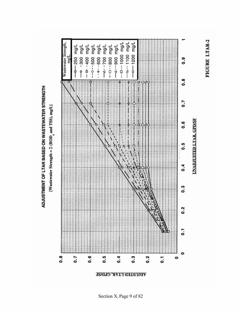
LTAR = 5K - [1.2/(Log10K)]. In this formula LTAR is in units of gpd/ft2 and K, saturated hydraulic conductivity, is in units of ft/minute. Figure LTAR-1 presents this expression in graphical format. For effluent from household septic tanks, the maximum stable LTAR value allowed by the CTDEP is 0.80 gallons per day per square foot of effective leaching area. This corresponds to a K value of ~28 ft/day (0.0197 ft/min. or 0.010 cm/sec). Siegrist (1987) stated that the rate of discharge from a SWAS to the underlying unsaturated zone should not exceed 3% to 5% of the saturated hydraulic conductivity. He stated that such low discharge rates (hydraulic loading rates) are required in order to maintain adequate soil aeration and the low soil moisture content in the unsaturated zone that will allow intimate contact between the percolate from the SWAS and the soil particles. These conditions are required for removal/attenuation of pathogens and other contaminants in the percolate. The LTAR rates obtained from Figure LTAR-1 satisfy this requirement. Laak (1970) hypothesized that the service life of a SWAS is related to the sum of the BOD5 and TSS and that increasing the pretreatment of domestic wastewater prior to discharge to a SWAS would increase the service life of the SWAS. Based on the results of his studies at the University of Toronto (Laak-1966), he suggested an expression for the affect of BOD5 and TSS in septic tank effluent on the development of the clogging mat at the SWAS-soil interface (Laak-1977). This expression could be used to calculate the increase in infiltrative surface area required for strong wastewater or the decrease in such area where reliable enhanced pretreatment is provided. An “adjustment factor”, based on the Laak expression, can be used to determine the leaching surface application rate to be used for high-strength (or low strength) wastewater. This factor is derived from the mathematical expression shown below (Laak-1977), which relates the five-day Biochemical Oxygen Demand (BOD5) and Total Suspended Solids (TSS) concentrations in such wastewaters, to the average concentrations of BOD5 and TSS found in the effluent of septic tanks receiving household wastewater:
LTAR Adjustment Factor = [250/(BOD5 + TSS)]1/3 In the preceding mathematical expression, the BOD5 and TSS are expressed in milligrams per liter, and represent the values of these constituents in the pretreated wastewater discharged to the SWAS.

Section X, Page 5 of 82

Section X, Page 6 of 82
Thus, for wastewaters having BOD5 and TSS values higher (stronger) than normal domestic wastewater, the LTAR value is decreased, and for wastewaters having lower (weaker) values, the LTAR value is increased. Where the septic tank effluent does not receive additional treatment prior to discharge to a SWAS, the maximum LTAR recommended = 0.8 gpd/sf of effective infiltrative area (ELA). Where additional treatment is provided, the maximum LTAR value recommended is 1.2 gallons per day per square foot of effective bottom area only. This limiting value is used to ensure the unsaturated soil conditions necessary in the soil beneath the SWAS for effective removal/inactivation of bacteria and viruses. 2. Results of Additional Research Considerable research has been conducted since the current method for determining LTAR was developed. (Anderson, et al-1981; Otis, R.J.-1984; Siegrist, et al-1984a&b; Siegrist-1987a & b; Tyler and Converse-1989; Jensen and Siegrist-1991; Tyler and Converse-1994; Loudon, et al-1998; Loudon-1999; Matejcek, et al-2000; Erlsten and Bloomquist-2001; Tyler-2001). Of considerable interest with respect to long term acceptance rates for wastewater strengths considerably higher than household wastewater are the very recent studies by Matejcek, et al-2000 and Erlsten and Bloomquist-2001. Matejcek et al (2000) conducted a thorough and well-documented study on long term acceptance rates for restaurant wastewater. Wastewater physical and chemical characteristics were determined for 133 samples of septic tank effluent from fifteen randomly chosen restaurants in Florida. Failure occurred primarily in the lysimeters with two feet of unsaturated soil that were dosed with medium and high strength wastewater. Twenty-four lysimeters failed during the 112-day study with 20 failures occurring between 20 and 47 days. No failures were recorded in lysimeters dosed with low strength wastewaters, which received a daily mass loading (BOD5 and TSS) of 0.0015 lb/ft2/day. In addition, the cumulative mass loaded on the low strength columns exceeded the cumulative mass loading of the failed columns dosed with medium strength wastewater. Conclusions reached by Matejcek et al. (ibid.) with respect to long term acceptance rates for restaurant wastewater were as follows: 1. Hydraulic loading alone does not cause drainfields to fail. Effluent concentration
and hydraulic loading both contribute to clogging and formation of biomat, resulting in failure.
2. Fine sand soil columns receiving less than 0.0015 lb/ft2/day of contaminant mass
(sum of BOD and TSS) did not fail. Similar columns receiving 0.0043 lb/ft2/day did fail. Therefore, there is a possible threshold at which drainfields fail due to daily mass loading. In this case, it appears to be between 0.0015 and 0.0043 lb/ft2/day for the fine sand soil.

Section X, Page 7 of 82
A similar case can be made for all four soil types. Below the thresholds, drainfields appear to be able to adequately treat the daily load and are poised for the next application with no apparent permanent failure.
Recommendations made by Matejcek et al. (ibid.) with respect to long term acceptance rates included: 1. Limits should be established for restaurant effluent with concentrations to be in
the low wastewater strength category (similar concentrations to those of wastes from domestic systems).
2. Drainfield sizing should include mass loading rates and hydraulic loading rates
based on soil properties. Mass loading rates should not exceed 0.0015 lb/ft2/day, but this value may need to be reduced based on soil properties.
However, Erlsten and Bloomquist (2001) reported on subsequent phases of the University of Florida’s Onsite Sewage Treatment and Disposal Systems and Long Term Acceptance Rate study. In phase 2, the mass loading threshold was shown to lie between 0.0015 and 0.0024 lb/ft2/day of combined CBOD5
(carbonaceous BOD5) and TSS loading. The purpose of the phase 3 study was to further refine the apparent threshold above which lysimeter failure occurred consistently. The results obtained from the phase 3 study confirmed the upper limit established in the phase 2 study. 3. Calculating LTAR The data on which Healy and Laak based their LTAR expression was obtained from residential sites discharging to stone filled trenches and were adjusted to a one foot ponding depth. If the infiltrative surface area hydraulic loading rates determined from the Healy and Laak LTAR expression are to be used for design of large scale on-site systems receiving a higher organic strength wastewater, the organic loading rates should be adjusted to that of household septic tank effluent. If it is assumed that the “strength” of household septic tank effluent (concentrations of BOD5 + TSS) = 250 mg/L, the equivalent “strength” loading, at 1 gpd/ft2, = 91 lbs./acre/day or 0.0021 lbs/ft2/day. At the maximum allowable LTAR (hydraulic loading rate) of 0.8 gpd/ft2, this equivalent loading rate becomes 72.6 lbs/acre/day, or 0.0017 lbs/ft2/day. This falls within the mass loading threshold range of 0.0015-0.0024 lbs/ft2/day found by Erlsten and Bloomquist (2001). The upper end of that range (0.0024 lbs/ft2/day) would be representative of a wastewater strength of about 360 mg/L. The mid-point of that range is 0.0020 lbs/ft2/day. The 250 mg/L value for the sum of household septic tank BOD5 + TSS came from Laak (1977) and apparently was based on household wastewater characteristics determined several decades ago. Additional data that has become available since that time appears to indicate that this value may be a little low. This may be partially due to the reduced flow fixtures that have been on the market for almost two decades, including both the 3.5 gallon per flush toilet and the newer 1.6 gallon per flush toilet, plus reduced flow lavatory and shower head fixtures. This reduction in flow can be expected to result in a corresponding increase in the septic tank effluent pollutant concentrations. However, a decrease in flow should show an increase in septic tank efficiency, and thus the effects of decreased flow may cancel each other.

Section X, Page 8 of 82
A method has been developed for adjusting the LTAR by using the Laak formula with the values obtained therefrom truncated when they exceed a mass loading of 0.0020 lbs./sf/day. A graph entitled “Adjustment of LTAR based on Wastewater Strength” is shown in Figure LTAR-2. The adjusted LTAR determined from Figure LTAR-2 is then further adjusted on the basis of the concentration of TN anticipated to be found in the pretreated wastewater discharged to the SWAS. This will account for the increased oxygen demand (nitrogenous oxygen demand) exerted by the bacteria that oxidize the TN to nitrates where the TN concentration exceeds the TN concentration found in household wastewater. Thus, where the TN concentration in the pretreated wastewater is greater than 56 mg/L, the adjusted LTAR based on wastewater strength is multiplied by the following factor:
TN adjustment factor = 56 mg/L[typical septic tank effluent] Pretreated Wastewater TN concentration, mg/L.
[The 56 mg/L is based on an upper limit of TN for raw residential wastewater of 70 mg/L and a removal rate of 20% in the septic tank. (70 mg/L *(1-0.20) = 56 mg/L)] The procedures discussed above provide a means for determining the infiltrative surface loading rates based both on hydraulic and organic loading rates.
Section X, Page 9 of 82

Section X, Page 10 of 82
D. Effective Leaching Surface Area 1. General The effective leaching (infiltrative) surface area (ELA) of a SWAS is the interface area between the soil and the facilities used for applying the pretreated wastewater to the soil. The wastewater application facilities, commonly referred to as leaching systems, may consist of: 1) flow distribution piping embedded in a coarse aggregate (commonly referred to as
stone, broken stone or “gravel”) filled trench, 2) a row, or rows, of precast concrete gallery units or plastic chamber units with open
bottom and coarse aggregate placed along the sides of the units and flow distribution piping installed within the units,
3) flow distribution piping embedded in a coarse aggregate leaching bed, but only where enhanced pretreatment is provided, or
4) other wastewater leaching units that are approved by the Department. As previously discussed under subsection C, the Healy and Laak expression for LTAR was based on a stone-filled trench ponded to a depth of one foot. Thus, the unit value (per linear ft. of trench) for ELA was the trench bottom contact area plus the sidewall contact area (one ft of height on each side of the trench). Several investigators have determined that, where gallery or chamber units are installed without coarse aggregate placed between the units and the soil interface (so called “gravel-less leaching systems”), infiltration of the pretreated wastewater into the soil is considerably more efficient. They attribute this increased efficiency to the lack of the “masking (shadowing) effect” of the broken stone or natural gravel. The masking effect on the infiltrative surface area by stone or gravel has been discussed for many years (Bouma and Magdoff -1974; Siegrist - 1987; Tyler, Converse and Milter-1991, Siegrist and Van Cuyk. 2001.). Recent studies have indicated that gravel-less leaching systems can be loaded at rates equal to 1.7 to 2.0 times the loading rate of systems using gravel. (Hoxie and Frick-1984; Tyler, Converse and Milter, ibid; Siegrist and Van Cuyk, ibid). On the other hand, while White and West (2003) agreed that gravel-less systems are more efficient in permitting the infiltration of wastewater through the biomat, they disagreed with the masking concept. The results of their studies indicated that it is the fines associated with the “gravel” aggregate that eventually slough off the aggregate and accumulate at the infiltrative surface that cause a reduction in leaching capacity. Their premise was later refuted by Siegrist, et al. (2004). Amerson and others (1991) stated “the presence of fines is the predominant factor in infiltration rate reductions. One to four percent of gravel fines by weight resulted in a significant reduction in infiltration rates by 35 to 65 percent.” While most state regulatory agencies require that the “gravel” be washed prior to use, in practice washed gravel is not always used. Even after washing, gravel used in constructing a SWAS still contains a small amount of fines (typically 3 to 5 percent), ranging in size from 2 mm to less than 20 µm. Over a short period of time, the fines wash from the gravel and settle at the bottom of the trench. Fines are a significant problem as they significantly reduce flow rates (White and West-ibid.).

Section X, Page 11 of 82
Regardless of whether it is the lack of fines, the absence of the “masking effect”, or both, that results in the observed increase in infiltrative efficiency of gravel-less systems, the increase appears to have been validated by several detailed studies. Therefore, the Department has determined that “gravel-less” systems can be allowed a higher ELA than that allowed for a leaching system where gravel is used and has adopted a factor of 1.5 for computing the unit value for ELA for gravel-less leaching systems. 2. Calculation of Effective Leaching Area (ELA) The following formula should be used to calculate the unit value for ELA/lf. The formula takes into account both masked and unmasked infiltrative surface areas, the hydraulic head on the infiltrative surfaces and an allowance for reserve storage area.
ELA/lf = [1.5 x inside clear (unmasked) bottom area of leaching unit + 1.0 x effective stone-masked bottom area] + [1.0 x effective height of stone-masked sidewall areas of leaching units*]
Where: Leaching Unit = stone-filled trench, concrete gallery unit,
plastic chamber unit, or other type of unit approved by the Department
Effective Sidewall Height = from Leaching Unit bottom to wastewater
inlet invert, in ft, but not more than one foot (30 cm).
* For gallery and plastic chamber units, inclusion of sidewall height in calculating the ELA will
only be permitted if the wastewater can flow into the sidewall areas through openings in the sidewalls that are less than one foot from the bottom of the unit.
Stone-masked Sidewall ELA, sf/lf = 2 x Effective Sidewall Height, in ft.
Stone-masked Bottom ELA, sf/lf = Bottom contact area of stone placed beneath
or on sides of Leaching Unit (1 ft. maximum either side of Leaching Unit), in ft. (Maximum allowable width of Leaching Unit plus sidewall stone = 6 ft)
Where a stone-bottomed leaching bed is used in a Lateral Sand Filter, the entire bed bottom area should be considered stone masked.
Unmasked Bottom Area, sf/lf = average inside clear bottom area of Leaching
Unit/lf. [It is acknowledged that additional sidewall height will provide additional ELA when the depth of ponding above the bottom of a Leaching Unit exceeds one ft (30 cm); however this is considered to be a safety factor and is not used in computing the unit value for ELA.]
Section X, Page 12 of 82
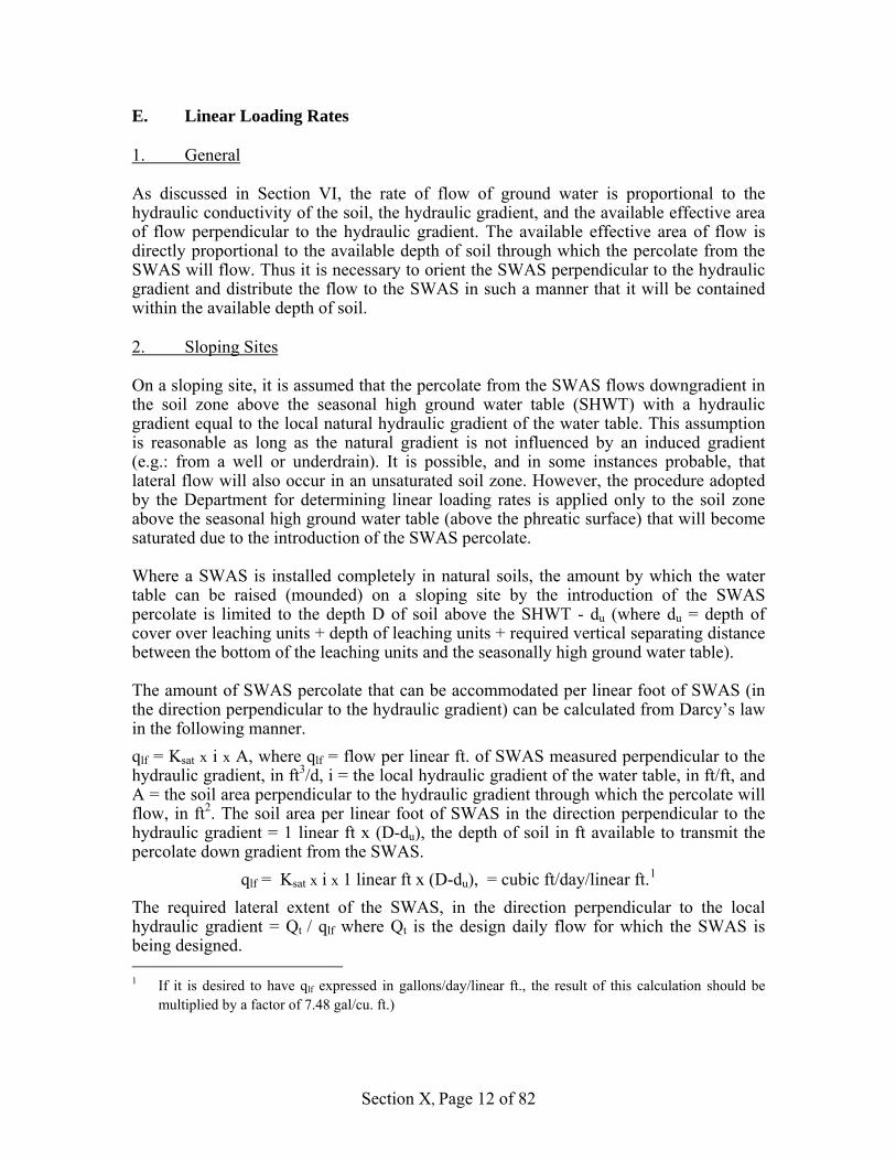
E. Linear Loading Rates 1. General As discussed in Section VI, the rate of flow of ground water is proportional to the hydraulic conductivity of the soil, the hydraulic gradient, and the available effective area of flow perpendicular to the hydraulic gradient. The available effective area of flow is directly proportional to the available depth of soil through which the percolate from the SWAS will flow. Thus it is necessary to orient the SWAS perpendicular to the hydraulic gradient and distribute the flow to the SWAS in such a manner that it will be contained within the available depth of soil. 2. Sloping Sites On a sloping site, it is assumed that the percolate from the SWAS flows downgradient in the soil zone above the seasonal high ground water table (SHWT) with a hydraulic gradient equal to the local natural hydraulic gradient of the water table. This assumption is reasonable as long as the natural gradient is not influenced by an induced gradient (e.g.: from a well or underdrain). It is possible, and in some instances probable, that lateral flow will also occur in an unsaturated soil zone. However, the procedure adopted by the Department for determining linear loading rates is applied only to the soil zone above the seasonal high ground water table (above the phreatic surface) that will become saturated due to the introduction of the SWAS percolate. Where a SWAS is installed completely in natural soils, the amount by which the water table can be raised (mounded) on a sloping site by the introduction of the SWAS percolate is limited to the depth D of soil above the SHWT - du (where du = depth of cover over leaching units + depth of leaching units + required vertical separating distance between the bottom of the leaching units and the seasonally high ground water table). The amount of SWAS percolate that can be accommodated per linear foot of SWAS (in the direction perpendicular to the hydraulic gradient) can be calculated from Darcy’s law in the following manner. qlf = Ksat x i x A, where qlf = flow per linear ft. of SWAS measured perpendicular to the hydraulic gradient, in ft3/d, i = the local hydraulic gradient of the water table, in ft/ft, and A = the soil area perpendicular to the hydraulic gradient through which the percolate will flow, in ft2. The soil area per linear foot of SWAS in the direction perpendicular to the hydraulic gradient = 1 linear ft x (D-du), the depth of soil in ft available to transmit the percolate down gradient from the SWAS.
qlf = Ksat x i x 1 linear ft x (D-du), = cubic ft/day/linear ft.1 The required lateral extent of the SWAS, in the direction perpendicular to the local hydraulic gradient = Qt / qlf where Qt is the design daily flow for which the SWAS is being designed. 1 If it is desired to have qlf expressed in gallons/day/linear ft., the result of this calculation should be
multiplied by a factor of 7.48 gal/cu. ft.)

Section X, Page 13 of 82
The total effective leaching surface area required per linear foot of SWAS = qlf/LTAR (with LTAR adjusted as may be required by wastewater strength). The number of rows of leaching units required for the SWAS then depends upon the effective leaching surface area of the selected leaching units or trenches. The procedure for determining the required lateral extent of a SWAS is illustrated in the following example, using U.S. units. Refer to Figure LL-1. EXAMPLE: A SWAS needs to be designed for a facility that will generate a maximum day flow (Q) of 6000 gpd. The available site has the following characteristics: The width of the site perpendicular to the local hydraulic gradient = 280 ft. The depth to the seasonal high ground water table (SHWT) = 10 ft. The local natural hydraulic gradient = 0.09 ft/ft. It is proposed to use leaching galleries having a height of 1.5 ft and to provide 1 ft. of cover over the top of the leaching galleries. In this example, the required vertical height of unsaturated soil below the bottom of the leaching galleries and the mounded seasonal high ground water table = 3 ft. du = 1.0 ft. + 1.5 ft + 3.0 ft. = 5.5 ft D-du = 10 ft - 5.5 ft = 4.5 ft. (Note that this is the maximum allowable height of
mounding above the seasonal high ground water table due to discharge of the percolate from the SWAS).
The design Ksat of the existing unsaturated soil, from 5.5 ft. below the ground surface to the SHWT was determined to be 8.0 ft/day. The allowable linear loading rate, qlf = 8.0 ft/day x 0.09 ft/ft x 1 lf x 4.5 ft. = 3.24 cu.
ft./day/lf. x 7.48 g/cu. ft. = 24.2 gpd/lf The required width of SWAS perpendicular to the local hydraulic gradient = Q/qlf = 6000 gpd/24.2 gpd/lf = 248 lf. Since the lot width is 280 ft, there appears to be ample room to install the SWAS, absent any local requirements for property line setbacks that may restrict the width of the SWAS. (Of course, the ability to use this site will also depend upon having sufficient distance between the SWAS and the closest point of concern to meet the travel time requirements, the phosphorus attenuation capabilities of the soils, the ability to meet the TN requirements at the closest point of concern and the ability to provide adequate hydraulic and infiltrative reserve.) Examples where the existing natural soils do not have sufficient capability to conduct the percolate away from the SWAS are given in the sub-section on Fill Systems.

Section X, Page 14 of 82
Section X, Page 15 of 82
3. Sites With Very Low Hydraulic Gradients On a site where the local hydraulic gradient is very low, a 3-Dimensional Hydraulic Capacity analysis is required, as discussed in Section VI. The approach to determining ground water mounding under such conditions is different from that used where there is a significant slope to the hydraulic gradient. In the low hydraulic gradient situation, a configuration of the SWAS must be assumed and the resulting mound height calculated to determine if there will be at least 3 ft. of unsaturated soil beneath the bottom of the SWAS and the SHWT. This may involve several iterations before the final configuration of the SWAS is selected. The following example, using U.S. units, indicates how the ground water mounding under such conditions may be calculated. EXAMPLE: (Refer to Figure LL-2.) A SWAS needs to be designed for a facility that will generate a maximum day flow (Q) of 6000 gpd. The available site has the following characteristics: The lot dimensions of the proposed site of the SWAS = 400 ft wide perpendicular to the hydraulic gradient and 600 ft long in the direction of the hydraulic gradient. The depth from ground surface to the seasonal high ground water table (SHWT) = 8 ft. The depth from the SHWT to the limiting horizon = 12 ft. The local natural hydraulic gradient = 0.001 ft/ft. and is considered to be negligible for the purposes of this example. The soils beneath the site consist of sands that extend from about 2 ft. below ground level down to the limiting horizon, which is bedrock. A water table exists above the bedrock at all times of the year. It is proposed to use 2.5 ft. high by 4.0 ft wide x 8.0 ft. long precast concrete gallery units with one foot of broken stone alongside the gallery sides. The effective leaching area for these units is given as 9.25 sq. ft./lf. The tops of the galleries will be one ft. below existing grade. The required vertical height of unsaturated soil below the bottom of the leaching galleries and the mounded seasonal high ground water table = 3 ft. du = 1.0 ft. + 2.5 ft. + 3.0 ft. = 6.5 ft. D-du = 8 ft (the depth from ground surface to the SHWT) - 6.5 ft = 1.5 ft. (Note that this is the maximum allowable height of mounding above the seasonal high ground water table due to discharge of the percolate from the SWAS). The design value selected for Ksat of the existing sandy soil, from 3.5 ft. below the ground surface to the bedrock = 25 ft/day = 0.0174 ft./min. From Figure LTAR-1, the long-term acceptance rate = 0.77 gpd/sf of effective leaching area. The pretreated effluent is estimated to have concentrations of BOD5 and TSS typical of effluent from a domestic septic tank, and therefore no adjustment for the LTAR is required. The total effective leaching area required = 6,000 gpd/0.77 gpd/sf = 7792 sq. ft. The total linear feet of leaching galleries required = 7792 sf/9.25 sf/lf = 840 lf.

Section X, Page 16 of 82

Section X, Page 17 of 82
An initial trial layout of the SWAS assumes 3 rows of leaching galleries spaced at 18-ft c.c. The leaching galleries are fabricated in 8-ft sections. Thus, each row will consist of 35 sections, yielding a total of 105 sections with a total of 840 lf of leaching galleries. The center to center spacing between rows of leaching galleries = 18 ft, the width of each gallery row will be 6 ft (including a one ft. width of stone along the sidewalls) and the length of each row will be 35 sections x 8 ft./section = 280 ft. Thus, the overall footprint of the SWAS will be (2 x 18 ft + 6 ft.) x 280 ft = 42 ft x 280 ft. = 11,760 sq. ft. A computer program for an analytical model of ground water mounding beneath a ground water recharge basin (“Flow From Wells and Recharge Pits” - Ref. Section VI, Subsection H.3.) is used to assess the hydraulic capacity of the proposed site. The SWAS footprint is assumed to be equivalent to a ground water recharge basin of the same dimensions. The analytical model requires the following input: • Transmissivity of the aquifer (saturated soil) material. (This is equivalent to the
hydraulic conductivity, (K, ft/d) x the depth of the aquifer (ft).) In this case, the transmissivity is calculated to be 25 ft/day x 12 ft = 300 sq. ft./day. In this example the aquifer is assumed to be homogeneous, isotrophic, and of infinite areal extent.
• The dimensions of the equivalent recharge basin (width and length). In this case,
these dimensions are 42 ft. and 280 ft. respectively. • The hydraulic loading rate of the basin. In this case, the equivalent unit hydraulic
loading on the footprint area of the basin = 6,000 gpd/(42 x 280) sq. ft. = 0.51 gpd/sf = 0.068 cu. ft/day/sq. ft., or 0.068 ft/day.
• The duration the basin will be loaded, in days. In this case, loading periods equal to
10 years and 20 years were selected. • The incremental distance from the center of the basin along the mound profile in the
X and Y directions for which the mound height will be calculated. In this case, an incremental distance of 20 ft. was selected. (Note; this information is useful for computing travel times to the closest points of concern, as the slope of the mounded water table (the hydraulic gradient) will vary with distance from the center of the SWAS.)
• The depth from ground surface to the (seasonally high) water table. In this case, 8 ft. • This data, when entered into the analytical model indicated a mound height of 1.8 ft
would develop beneath the SWAS during the first ten years of loading and a mound height of 2.0 ft would occur after 20 years of loading. This indicates the mound height will probably not significantly exceed 2.0 ft. over a very long time period.
Since the calculated maximum height of the mound is 2.0 ft, which is greater than D-du (1.5 ft), the design is unsatisfactory with respect to the required 3 ft of vertical separating distance as the mounded water table will rise to 2.5 ft below the SWAS.

Section X, Page 18 of 82
It should be noted that additional assumptions of the SWAS footprint, type of leaching unit, etc. will allow iterations of the computer model to optimize the design with respect to SWAS dimensions, length and number of gallery rows, etc. A comparison of the results obtained from the analytical computer model was made with the results obtained from the simple well formula given in Section VI. This formula is:
Q = (π k (H2 -h2))/ln (R/r) = (π k (H2 -h2))/2.3Log10 (R/r) Where :
k = saturated hydraulic conductivity (ft/d), H = height of the ground water mound above an impermeable lower boundary at a
distance r from the center of the recharge basin (ft), h = the original saturated thickness of the aquifer (ft), R = the radial distance (ft) from the center of the recharge basin to an aquifer
boundary or an assumed outer limit of the mound (where H ~ h), and, r = the radial distance (ft) from the center of the recharge basin to a point on the
mound for which H is calculated. The bottom area of the SWAS was calculated to be 11,760 sq. ft. The radius of a circular area having the same bottom area = (11,760 /π)0.5 = 61 ft. In order to compare the results of the simple well formula with the analytical computer model, the value of R must be large enough to simulate an aquifer of infinite lateral extent2. Therefore, R has arbitrarily been assumed to be 100 x the equivalent radius of the recharge basin; i.e. 100 x 61 ft = 6100 ft. The value of r has been assumed as five feet; that is, the value of H will be computed at a distance of 5 feet from the center of the equivalent circular recharge basin.
2.3 x log10 (R/r) = 2.3 x log10 (6100/5) = 7.1. From Figure LL-2, h = 12 ft. [H2 - h2] = Q x 2.3 x Log10 R/r = 802 ft/day x 7.1 = 72.5 ft2 πK π x 25 ft/day
H2 = 72.5 + (12)2 = 216.5 ft2. H = 14.7 ft. and the mound height = H-h = 14.7-12 = 2.7 ft.
Thus, the simple well formula predicts that the mounded SHWT will rise to 8 ft. - 2.7 ft. = 5.3 ft below the ground surface. This will only be 1.8 ft below the bottom of the SWAS, which is not acceptable. On the other hand, the analytical computer program predicts that the mounded SHWT will rise to 6.0 ft (8.0 ft.-2.0 ft.) below the ground surface, which is also unacceptable, as there will only be 2.5 ft of unsaturated soil beneath the SWAS. Thus, in both cases, fill would be required to provide the required 3 ft vertical separating distance. In this example, the results of the two methods of mounding analysis are similar; that is, the site does not have sufficient hydraulic capacity to provide the required 3-ft. vertical separating distance. In other cases the results might be different. For example, had the depth from ground surface to the SHWT been 9.0 ft instead of 8.0 ft., the results from the 2 It should also be noted that the results from the simple well formula are somewhat sensitive to values of R assumed, except where it is known that H~h at the assumed value of R (i.e.: where R extends to a surface water body, open drainage ditch or ground water interceptor drain).
Section X, Page 19 of 82
analytical computer program would have indicated that the site had sufficient hydraulic capacity (i.e.: mounded SHWT at 3.5 ft below the bottom of the SWAS). However, the simple well formula would have indicated that the design was not suitable, as the mounded SHWT would have risen to 2.8 ft below the bottom of the SWAS. This illustrates the need to carefully consider the method to be used in estimating the height of the ground water mound beneath an SWAS. F. Fill Systems 1. General The principles set forth in sections II, III, and IV are also applicable to the design of fill systems. However, the design and construction of fill systems will require significantly more effort and the cost to design and construct such systems are likely to be very much greater than for systems installed in natural soils. There are also regulatory constraints on the use of fill, as discussed further in subsection F.7. 2. Types of Fill Systems Fill systems constructed to supplement natural soils are generally proposed where the existing soil is suitable with respect to hydraulic conductivity, wastewater renovative capacity, and depth to bedrock or other hydraulically restrictive layer, but a high ground water table will not permit the SWAS to have the required vertical separating distance above the mounded seasonal high ground water table that will exist during system operation. In this case, the soil downgradient of the SWAS has adequate hydraulic capacity to conduct the percolate from the SWAS for a sufficient distance downgradient to meet travel time requirements, but fill is needed to elevate the area in which the SWAS will be installed. Fill systems constructed to replace natural soils are designated by the Department as Lateral Sand Filters, and are generally proposed in the following cases. Case a.1. The existing soil is suitable with respect to hydraulic conductivity and
wastewater renovation, but there is an insufficient depth of such soil above bedrock or other hydraulically restrictive layer (i.e. insufficient hydraulic capacity and insufficient unsaturated vertical separating distance).
Case a.2. An existing system has failed because the existing soil has inadequate
hydraulic capacity or wastewater renovative capacity (or both), or there is insufficient separating distance above the seasonally high mounded ground water table, or the ground water table is at or below the surface of the bedrock.
In the cases of a.1. and a.2, the soils below and downgradient of the SWAS have inadequate hydraulic and renovative capacity. Therefore, sufficient fill must be placed to provide the required three feet of unsaturated soil of suitable renovative capacity below the bottom of the SWAS, and to provide the additional hydraulic capacity to conduct the percolate from the SWAS for a sufficient distance downgradient to meet the travel time requirements. It will also be necessary to provide a hydraulic barrier between the bottom of the fill and the soil on which the

Section X, Page 20 of 82
fill is placed to ensure that the percolate from the SWAS does not reach a ground water table located at or below the surface of the fractured bedrock before it is sufficiently renovated. The reason for the barrier is addressed below.
In the absence of definitive and conclusive evidence to the contrary, the Department will assume that all bedrock is fractured (the predominant condition in Connecticut) or contains large solution voids or channels such as exist in the karstic bedrock areas in northwestern Connecticut. Where the existing soils have adequate hydraulic capacity but a high water table requires the use of fill to provide the required vertical separating distance, it is assumed that the percolate will flow downward through the unsaturated zone until it reaches the water table3 in the soil above the bedrock and then will flow laterally in the direction of ground water flow in response to the hydraulic gradient. This assumption is considered reasonable because vertical mixing of the percolate with the ground water is usually slow and limited to several feet. Therefore, vertical movement of the contaminants remaining in the percolate into the bedrock aquifer can be ignored. However, there is a need to be very careful where the soils are shallow to bedrock and where the seasonal ground water table is in the bedrock. This situation is represented by cases a.1. and a.2. and is often found on the crest of hills and ridges. The soil mantle at these locations often consists of well-drained or excessively well-drained soils or has inclusions of such soils that allow infiltrating water to rapidly reach the bedrock aquifer. Under these conditions, it is probable that any pathogens and pollutants remaining in the percolate from the SWAS after it flows through the unsaturated zone could easily reach the bedrock aquifer. In such cases, it is difficult to determine the travel time of the percolate and a conservative assumption is made that it can travel quite rapidly through the bedrock fractures to a point of concern due to uncertainty in fracture distribution and orientation. In addition, the percolate in such cases will not receive the additional renovation normally provided by horizontal travel through a suitable soil aquifer for a sufficient period of time. Thus, the percolate must be prevented from entering the fractured bedrock until it has met the prescribed travel time requirement of the Department. Where it is necessary to locate an OWRS in such an area, a hydraulic barrier beneath the entire fill system may be required. Another situation that needs careful attention is when the seasonal high water table is above the bedrock, but the water table recedes into the bedrock during the drier portions of the year. In this case, the bedrock aquifer can become contaminated in the same manner as described above. Where initial subsurface investigations indicate the absence of a water table in the soils or unconsolidated substratum, further investigations should be 3 However, some investigators (e.g. Crosby, et al -1968; Pask -1988, 1994; and Mooers and Waller-1996) have shown that under certain conditions lateral flow will also occur in the unsaturated zone.

Section X, Page 21 of 82
conducted during the driest period of the year.4. (However, such investigations might be problematic if significant rainfall events occur in the normally driest portion of the year.) If these further investigations confirm that the water table may recede into the bedrock any time during the year, the Department may require that an approved hydraulic barrier be provided beneath the entire fill system. Where a hydraulic barrier is required, the hydraulic conductivity and thickness of the barrier soil must be such that the vertical travel time through the barrier and any existing soil or substratum materials below the barrier will be equivalent to the travel times prescribed by the Department elsewhere in this document. 3. Requirements for Fill Material Where fill is required only to provide vertical separation between the bottom of a SWAS and the seasonal high ground water table (leaching fill), the required vertical saturated hydraulic conductivity (Ksat.) of the fill material, after placement and compaction, is based on the unit hydraulic loading rate selected for design (e. g,: if a hydraulic loading rate of 0.8 gpd/sf, the maximum LTAR permitted, is selected for design of a SWAS, a Ksat. value ≥ 29 ft/day is required). Coarse sand, as defined in Appendix B, should not be used for leaching fill. It is also important that the vertical hydraulic conductivity of the fill should not be significantly lower than that of any soil horizon on which it is placed. If this should occur, it is possible for the fill with the lower K value to become saturated with the percolate from the SWAS before the percolate will flow downward through the fine soil-coarse soil interface. This situation can occur due to the soil moisture tension (matrix potential) being greater than the gravitational potential. In such cases, water will not cross the boundary between the upper fine soil and the lower coarser soil until the voids (capillaries) in the fine soil are filled. In such circumstances, it is likely that the requirement for unsaturated soil conditions would not be met in the fill. Thus, the use of soils having predominantly small particle sizes (e.g. fine sands, loamy sands and sandy loams) for fill material placed above coarser textured soils becomes problematic, and should be avoided. Where fill is required to provide the saturated hydraulic capacity to conduct the flow laterally from the bottom of the unsaturated zone for a distance sufficient to meet the travel time requirement of the Department, the hydraulic conductivity required will be based on the linear loading rate, the slope of the mounded seasonal high ground water table, the depth of the fill and the SWAS configuration. In this case, the designer can adjust any or all of these parameters to obtain a cost-effective system, although the adjustments are usually constrained by site features such as existing ground slope, the width and length of the site, and the characteristics of available fill materials. By making several trial analyses, the designer can determine the required hydraulic conductivity of the fill. 4 The presence of a permanent water table above bedrock may be indicated by the presence of a soil horizon with a gleyed (gray to bluish hue, chroma color ≤ 2) matrix. However, some low chroma colors may occur in unsaturated materials that contain little to no oxidized iron; this may more often be the case in sandy soils (fine-grained soils usually contain some iron). In such cases, the soil may or may not be permanently saturated. Therefore, it is important that saturation be confirmed by other means than soil color before assuming that the presence of gleyed soil indicates continual soil saturation.

Section X, Page 22 of 82
Where fill is required to meet vertical separation and lateral travel time requirements, it is possible that two types of fill material might be required. One type of fill would be required for the unsaturated zone beneath the SWAS and another for the fill in the saturated zone beneath and down-gradient of the SWAS. Ideally, suitable fill material would consist of a medium sand with a small amount of silt and clay particles having a sufficient reactive mineral content to which the contaminants in the percolate that are not removed by filtration can be sorbed as discussed in Section II of this document. It is this sorption that plays a large role in the ability of the soil to remove or attenuate pathogenic, organic and inorganic contaminants. However, in practice, medium sand with any significant amount of fine particles would have a significant reduction in hydraulic conductivity when the fill is placed and compacted (Ref: Subsection D of Section VI of this document). Thus the selection of fill material almost always involves a compromise between adequate hydraulic conductivity and adequate renovative capacity. It has been found that, to avoid significant reduction of hydraulic conductivity due to compaction of the fill, the percentage (by weight) of fine particles passing the 100 and 200 mesh sieves should be limited to 6% (≤ 4% is preferable) and 3% respectively. In addition, the fill should not be too well graded from coarse to fine, as such material will tend to pack tightly when compacted, resulting in low values of Ksat. Thus, the use of fill materials with a uniformity coefficient (d60/d10) > 4 should be avoided. It should be noted that in most cases, fill meeting the above requirements is obtained from commercial pits that extend a considerable distance below the soil solum (A and B horizons). In many cases, the fill is obtained near the bottom of the pits, where the deposition of colloids, soluble salts, and mineral particles by the process of illuviation has not occurred to a significant extent. In such cases, the sand may not have the phosphorus removal properties of the soils that lie closer to the ground surface. Therefore it will be necessary to evaluate the ability of such fill materials to sorb phosphorus, rather than use P sorption capacity values contained in the literature or given in Section II of this document, which are normally based on soils obtained from the soil solum. To determine phosphorus removal capabilities of proposed fill material, laboratory batch equilibrium experiments should be conducted to generate phosphorus adsorption isotherms on which the phosphorus sorption capacity (mg P sorbed/100 g of soil) can be based. The particle size distribution of the fill material should be determined by sieve and hydrometer analyses (e.g. ASTM Standard Test Method D 422) for a number of proposed fill samples. It is recommended that the nest of sieves used should include those U.S. Standard Sieve sizes that will permit soil classification in accordance with the U. S. Department of Agriculture Natural Resources and Conservation Service (NRCS-formerly the SCS) soil texture classification method. This method classifies soils by particle size as shown in the following table.

Section X, Page 23 of 82
TABLE FS-1
NRCS SOIL CLASSIFICATION BY PARTICLE SIZE RANGES
Classification Particle Size Range, mm gravel 2.0-75.0 very coarse sand 1.0-2.0 coarse sand 0.5-1.0 medium sand 0.25-0.50 fine sand 0.10-0.25 very fine sand 0.05-0.10 silt 0.002-0.05 clay <0.002
A nest of sieves that includes the 3”, 3/4”, #4, #10, #18, #35, #60, #100, and #200 standard sieves will provide data for a plot of a particle size distribution curve. This data will aid in classification of the soil in conformance with the NRCS soil texture method for all but the silt and clay fractions. The hydrometer analysis will provide information on the relative amount of silt and clay present. The information obtained from sieve analyses and hydrometer analyses can also be used to define the soil texture, using the soil textural classification system adopted by the NRCS (See Appendix B). The fill material must be placed in layers (lifts) not to exceed 12 inches in loose depth and compacted to a specified density. If this is not done, the hydraulic conductivity of the fill eventually will be significantly reduced due to settlement caused by gravitational affects and the affect of infiltrated precipitation. If each layer of fill is compacted to at least 90% of maximum density5, it is unlikely that any further compaction will occur. (N.B. However, where fill is placed in areas subject to heavy wheel loadings, it should be compacted to 95% of maximum density.) The hydraulic conductivity of each layer of fill must therefore be determined after it has been placed and compacted. Initial testing of representative fill material samples should be conducted by a soil testing laboratory by compacting the material to at least 90% of maximum modified Proctor density in order to determine the hydraulic conductivity of the material after compaction. After the samples have been adequately compacted, tube samples of the compacted material should be taken and the hydraulic conductivity determined as discussed in Section VI of this document. Because of the inherent variation in soil properties and test results, there will be a range of K values obtained from such tests. Therefore, the K values specified for the fill material should span a range that can reasonably be attained in the field. 4. Hydraulic Analysis Where fill is placed to increase the hydraulic capacity of a site, it will be necessary to carry out a hydraulic analysis to determine the thickness and lateral dimensions of the fill required. These hydraulic analyses will differ in detail and complexity depending upon the nature of the fill system. 5 As determined by the modified Proctor compaction test performed in conformance with ASTM D1557, Method D

Section X, Page 24 of 82
Case a. Fill required for adequate vertical separation distance above seasonal high
ground water table (Leaching Fill). In this case, the flow from the SWAS will basically be vertically downward through the fill (leaching fill) and existing subsoils until it reaches the water table. The depth of leaching fill that will be required will depend upon the calculated increase in the height of the seasonal high water table. For sloping sites, where the ground water table slope is similar to the surface slope, such calculations are similar to those shown for basic site hydraulic capacity analyses in Section VI, Subsection F 3 of this document. For cases where the existing ground water table is essentially horizontal, a three dimensional analysis will be required, as discussed in Section VI, Subsection G of this document. The lateral extent (width of the leaching fill) will depend upon the maximum lateral extent of the SWAS (parallel to the surface contours). The leaching fill should extend for a distance of at least five feet beyond the entire perimeter of the SWAS facilities to provide for some lateral dispersion of the percolate. The finished grade over the SWAS should have a slope of at least 2% to permit precipitation to flow off of the filled area. The depth of the leaching fill and any existing soil that will remain unsaturated must be such as to provide sufficient phosphorus sorption capacity as discussed in subsection G.4 of this section. A berm of compacted inorganic material (glacial till) having a relatively low hydraulic conductivity compared to the leaching fill material should be placed completely around the perimeter of the leaching fill material and should be toed into the existing surface for a depth of at least one foot. This berm should have a top width of at least five feet and of such additional width that may be necessary to accomodate compaction equipment. An example of such a system is shown in Figure FS-1. Case b. Fill Required for Providing Adequate Vertical Separation Distance Above
Selected Soil Horizons With respect to hydraulic capacity computations, Case b is a combination of Cases a and c and the methods described herein for those cases can be used for Case b. It should be noted, however, that there would be at least two soil horizons involved in conducting the SWAS percolate away from the SWAS. These would include the fill horizon and at least one existing soil horizon, and thus a different K value should be used to determine the hydraulic capacity of each horizon. Case c. Lateral Sand Filters. A fill system used to increase the hydraulic capacity of a site by constructing part or all of the system above existing grade has been designated as a Lateral Sand Filter (LSF) by the Department. Several lateral sand filters have been approved and constructed in Connecticut.

Section X, Page 25 of 82

Section X, Page 26 of 82
Hydraulic analyses for determining the thickness and lateral dimensions of the fill will differ in detail and complexity depending upon the nature and configuration of the system. A number of variables have to be considered in the design of a LSF, including: • length, width, height, and cross-section geometry, • the existing local hydraulic gradient, or the established hydraulic gradient, • the LSF site area, geometry and topographic constraints • the amount of existing soil above the bedrock on the site, • the position of the water table with respect to the bedrock, • the hydraulic capacity of the existing soil, • the landscape position of the LSF on the site, • the soil materials readily available, and the range of soil hydraulic conductivities, • the design flow and organic loading, • the configuration of the leaching system, • the required travel time of the SWAS percolate, • points of concern within and adjacent to the proposed site, and • Applicant’s ownership or control of zone of influence extending to a wetland or
surface water body. Many of these variables are interrelated; and as the values of one variable or more are changed, they will have an affect on the configuration of the LSF; (e.g., LSF length, width, depth and cross-section geometry and the hydraulic gradient). The LSF basically consists of the sand used to provide renovation of pretreated wastewater contained within a three-sided U-shaped berm, constructed of low permeability soil materials, that directs the flow of liquid in the LSF down-gradient to the open end of the system. The renovated wastewater then seeps from the toe of the sand fill as a non-point source discharge. The designer of a LSF has the ability to specify and control certain design parameters that could not be specified or controlled for a system constructed in native soils. For example, soil materials can be selected (and thus the hydraulic conductivity (K) values, within a reasonably close range) and, within site boundary and topographic constraints, the hydraulic gradient can be selected and the system configuration can be varied without concern for natural soil conditions, boundary conditions and topographic constraints. However, this latitude in design comes at a very significant cost. The cost to design and construct a LSF can be at least an order of magnitude greater than for similarly sized systems constructed in natural soils that have adequate hydraulic and renovative capacities. This is due to the fact that design of an LSF system is more complicated, and the construction and quality control testing is more difficult, as compared to what would be experienced for systems of equal capacity constructed in natural soils. Major cost factors are the importation of select fill materials, careful placement and compaction of the fill, the associated extensive laboratory and field testing that is required to obtain dependable data for design and during construction for quality control, and the extensive construction inspection that must be employed. The design of an LSF is more involved because the latitude in selecting design values may require a number of iterations of the design in order to arrive at one that is cost-effective and meets the water quality goals of the Department.

Section X, Page 27 of 82
In practice, however, there are other materials and components of the LSF that are required to insure the integrity of the system. These include, but are not necessarily limited to: • a low-permeability layer of soil beneath the sand. in certain instances, to confine the
pretreated wastewater to the sand fill, • pervious toe drains (usually constructed of geotextile fabric, broken stone and riprap)
at the outside toes of the berms and at the toe of slope at the downslope end of the sand fill to prevent slope failure due to excess pore water pressure,
• materials to stabilize the downslope end of the sand fill to prevent sloughing and erosion of the fill,
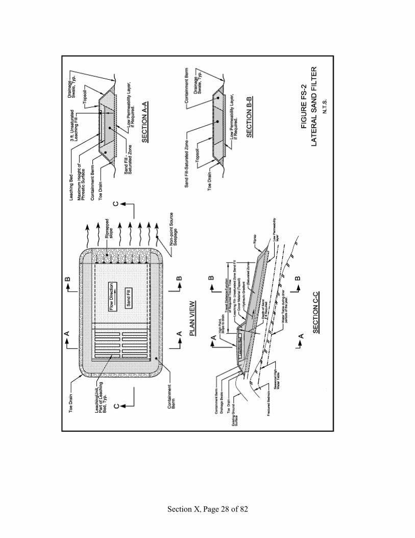
• vegetated topsoil for cover over the berms and top of the sand fill, and, • the materials required for the SWAS Figure FS-2 shows typical sections through a LSF. This figure depicts many of the conditions that may be encountered when the use of a LSF is being considered. Suggested steps for preliminary design of an LSF are given below. Unless otherwise stated, the hydraulic conductivity, K, is the horizontal saturated hydraulic conductivity of the soil materials. A. Design the portion of the LSF located down-gradient of the leaching fill area. The
objective here is to compute the required cross-sectional area of the saturated sand fill through which the design wastewater daily flow (Qdf), will flow to the down-gradient end of the LSF. Where a liner is required below the LSF, the design flow must also include the precipitation that infiltrates through the top of the LSF (Qpi). 1. Compute the total design flow, Qt.
This includes the design wastewater daily flow (Qdf) and, where a low permeability liner is required below the LSF, the precipitation that will fall on and infiltrate the LSF (Qpi). (A reasonable precipitation value might be based on the average daily precipitation during the maximum monthly precipitation that occurs late in the year, when the ground has not yet frozen but evapotranspiration is negligible. A conservative approach, with respect to the hydraulic calculations for the LSF, would be to assume that all of this precipitation infiltrates the top surface of the LSF). Qt is actually a variable because the amount of the infiltrated precipitation added to Qdf, as one proceeds from the up-gradient end to the downgradient end of the LSF, increases with the incremental increase of surface area as the flow proceeds downgradient. However, the total precipitation infiltrated through the top surface of the LSF is a relatively small part of Qt and therefore the entire amount of the precipitation infiltrating through all of the top surfaces of the LSF, (Qpi), can be added to Qdf. This will provide a small factor of safety when computing the required depth of the saturated sand fill.
Section X, Page 28 of 82

Section X, Page 29 of 82
2. Compute the total required effective leaching area (ELA) based on the leaching units selected.
3. Assume a layout of leaching units that will provide the required ELA and
determine the width of the required leaching area perpendicular to the hydraulic gradient and the length of the leaching area in the direction of the hydraulic gradient.
4. Assume a value of K for the compacted sand fill. (Ref: Appendix C.) 5. Assume a value for the hydraulic gradient.
While the designer has some latitude in selecting the hydraulic gradient, in most instances, the hydraulic gradient should be configured as closely as possible to the pre-existing topography to minimize construction costs. However, in some cases the distance from the leaching fill area to the downgradient property line, or other point of concern, may be constrained. It may then be necessary to reduce the hydraulic gradient and thus reduce the required travel distance since the travel distance is inversely related to the hydraulic gradient when K is held constant. Another means of reducing the travel distance is to select a fill material with a lower value for K for computing travel time. However, this will have an affect on the required flow area perpendicular to the hydraulic gradient.
6. Calculate the required flow area cross-section perpendicular to the hydraulic gradient. The required flow area is computed from the Darcy’s law Qt = K i A. Thus, A = Qt /(K i). (To get A in square feet, Qt must be in units of cubic ft/day and K must be in units of ft/day.)
7. Determine the geometry of the flow area cross-section, which will normally be in
the form of a trapezoid, with a bottom width smaller than the top width, due to the shape of the containment berms.
The side slopes of the trapezoid will be the same as the inside slope of the containment berms. A reasonable first assumption for these slopes is 2 horizontal to 1 vertical. The bottom width of the trapezoid (Wb) will equal the width of the required leaching area perpendicular to the hydraulic gradient as calculated in step No. 3. The area of the trapezoid, A = Wb H + 2H2, where H is the required depth of sand. Also, from Step No. 6 above, A = Qt/(Ki); therefore, Qt /(K i) = Wb H + 2 H2. All terms in this equation except H are known and H can be determined by solving the resulting quadratic equation.
8. The length of the LSF, of cross-section A, down-gradient of the leaching fill area
will depend upon the values of K used to calculate travel time, the slope of the phreatic surface, or hydraulic gradient, i, and the required travel distance.

Section X, Page 30 of 82
The required travel distance in the LSF downgradient of the leaching fill area (travel distance) = travel time required, in days, x (K i)/n. For most of this distance, the phreatic surface will have a constant gradient (i) and depth (H). The design values of K and n (porosity) used to compute travel distance are normally considered to be constant for the entire LSF. However, from a point near the crest of the sloping seepage face at the down-gradient end of the LSF to the point where the phreatic surface will intersect the seepage face, the phreatic surface will become steeper. The velocity in this portion of the LSF will be significantly higher than in the full fill section because of the increase in the slope of the phreatic surface as the flow approaches the seepage face. A flow net analysis in this portion of the LSF can be made that will define the steeper phreatic surface. This will enable calculation of the travel time from the crest of the slope to the point of seepage breakout at the face of the slope as a function of the increasing hydraulic gradient. However, a simpler method of defining the phreatic surface in this portion of the LSF can be used without significant error. This method assumes the phreatic surface to be a straight line drawn from a point on the phreatic surface beneath the crest of the slope to the toe of the sand fill. The slope of this line can be taken as the hydraulic gradient for computing the travel time increment in this portion of the LSF. The required length of the LSF, from the downgradient end of the SWAS to the crest of the slope at the downgradient end of the LSF, can then be computed using the required travel time less the aforesaid time increment and the procedure for computing travel distance given above.
B. Design the saturated portion of the LSF beneath the leaching fill area. The objective
here is to compute the required cross-sectional area and depth of the saturated sand fill through which the design wastewater daily flow (Qdf), plus precipitation that infiltrates through the leaching fill (Qpi) where a liner is used, will flow in a horizontal direction beneath the unsaturated portion of the leaching fill. There are several methods that can be used to compute the depth of the saturated sand fill.
1. One method of computing the depth of the saturated sand fill is to assume a
constant bottom slope for the saturated fill, as shown in Figure FS-3 A. Having established the depth of flow in the lateral sand filter downgradient of the leaching fill area, the depth of the leaching fill below the SWAS can be determined by calculation of the phreatic surface below the SWAS. Refer to Figure FS-3B, which is an enlargement of Section C-C shown in Figure FS-3A.
The phreatic surface profile below the SWAS leaching units is determined by the following form of Darcy’s Law: I = Qt/KA, where Qt = total design flow at any selected point on the profile, A = the cross-sectional area of flow at Qt, and K is the hydraulic conductivity for the sand fill. The phreatic surface profile is determined by summation of the qd and qpi values for each sub-area shown in Figure FS-3B and treating the flow as a line source at the centerline of each row of leaching units.

Section X, Page 31 of 82

Section X, Page 32 of 82

Section X, Page 33 of 82
Computation of the phreatic surface profile by the above equation is accomplished by assuming a constant bottom slope of the entire LSF fill, including that portion of the fill beneath the SWAS. Therefore, the hydraulic gradient required to conduct flow through the saturated sand cross-section varies linearly as a function of Qt. The resulting phreatic surface profile has a hydraulic gradient equal to that of the sand fill downgradient of the SWAS and the hydraulic gradient at the up-gradient end of the LSF approaches zero. The generalized procedure for making these computations is shown in Figure FS-3B.
2. Another method to compute the depth of the saturated sand fill is to assume a
constant hydraulic gradient for the full length of the LSF, as shown in Figure FS-3C. The generalized procedure for making these computations is shown in Figure FS-3D. In this method, the bottom slope of the fill beneath the SWAS will vary.
3. A third method is to vary both the depth of the saturated fill and hydraulic
gradient beneath the SWAS. This is a more involved procedure, requiring several iterations because of the two unknown variables, H and i, and may be of limited practical use.
C. Compute the depth of low permeability layer required beneath the LSF.
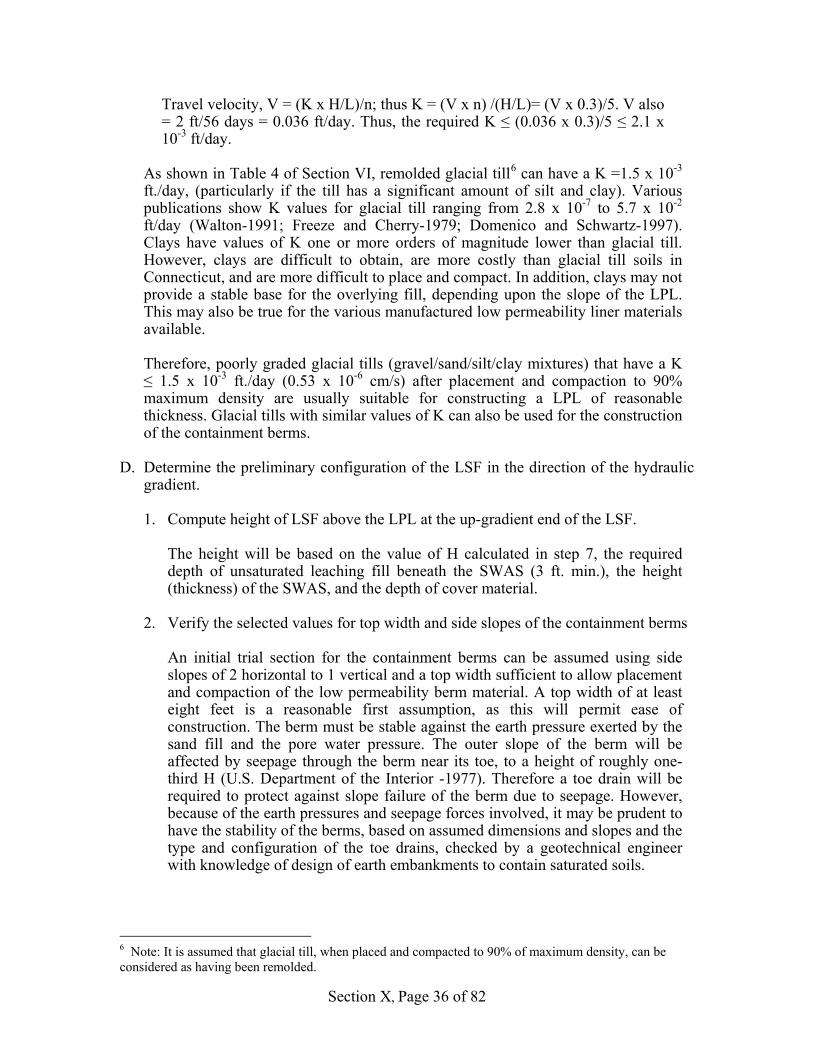
To calculate the required depth of the low permeability layer (LPL), if such a layer is required, the hydraulic gradient through the LPL and the vertical K of the layer must be known. The hydraulic gradient = H/L, where H is the height of the water table in the sand above the LPL and L is the thickness of the LPL. Therefore, the height of the water table, (H), above the LPL must first be determined. With H known from step A.7, the required minimum vertical K for the LPL based on an assumed value for L, and value of n can be calculated, or the required value for L can be calculated for an assumed known value of vertical K and n. Assuming a value of L for the LPL, which is also the travel distance corresponding to the required travel time, and having previously determined H, the hydraulic gradient through the LPL is known and the corresponding value for the vertical K may be calculated. The travel time through the LPL = V x T= [(K x H/L)/n] x T, where V = the linear velocity of flow through the LPL, T = the required travel time, and n = the porosity of the LPL. V x T also equals the required value L. Thus, L/T = (K x H/L)/n, and L = [T/n] x [K x (H/L)]. This equation for L cannot be solved directly, because it contains three unknowns, H, K and n. However, after determining the value of H from step 7, assuming a value for maximum allowable K and n will permit the calculation of L, or assuming a value for L and n, the maximum value for K can be determined. For example:
H for a particular LSF has been calculated to be ten feet. Assume the thickness of the LPL =2 ft =L. Then H/L = 10/2 = 5. Assume a reasonable porosity for glacial till is 0.3. Assume the required travel time is 56 days.

Section X, Page 34 of 82

Section X, Page 35 of 82
Section X, Page 36 of 82
Travel velocity, V = (K x H/L)/n; thus K = (V x n) /(H/L)= (V x 0.3)/5. V also = 2 ft/56 days = 0.036 ft/day. Thus, the required K ≤ (0.036 x 0.3)/5 ≤ 2.1 x 10⁻³ ft/day.
As shown in Table 4 of Section VI, remolded glacial till6 can have a K =1.5 x 10⁻³ ft./day, (particularly if the till has a significant amount of silt and clay). Various publications show K values for glacial till ranging from 2.8 x 10⁻⁷ to 5.7 x 10⁻² ft/day (Walton-1991; Freeze and Cherry-1979; Domenico and Schwartz-1997). Clays have values of K one or more orders of magnitude lower than glacial till. However, clays are difficult to obtain, are more costly than glacial till soils in Connecticut, and are more difficult to place and compact. In addition, clays may not provide a stable base for the overlying fill, depending upon the slope of the LPL. This may also be true for the various manufactured low permeability liner materials available. Therefore, poorly graded glacial tills (gravel/sand/silt/clay mixtures) that have a K ≤ 1.5 x 10⁻³ ft./day (0.53 x 10⁻⁶ cm/s) after placement and compaction to 90% maximum density are usually suitable for constructing a LPL of reasonable thickness. Glacial tills with similar values of K can also be used for the construction of the containment berms.
D. Determine the preliminary configuration of the LSF in the direction of the hydraulic gradient.
1. Compute height of LSF above the LPL at the up-gradient end of the LSF.
The height will be based on the value of H calculated in step 7, the required depth of unsaturated leaching fill beneath the SWAS (3 ft. min.), the height (thickness) of the SWAS, and the depth of cover material.
2. Verify the selected values for top width and side slopes of the containment berms
An initial trial section for the containment berms can be assumed using side slopes of 2 horizontal to 1 vertical and a top width sufficient to allow placement and compaction of the low permeability berm material. A top width of at least eight feet is a reasonable first assumption, as this will permit ease of construction. The berm must be stable against the earth pressure exerted by the sand fill and the pore water pressure. The outer slope of the berm will be affected by seepage through the berm near its toe, to a height of roughly one-third H (U.S. Department of the Interior -1977). Therefore a toe drain will be required to protect against slope failure of the berm due to seepage. However, because of the earth pressures and seepage forces involved, it may be prudent to have the stability of the berms, based on assumed dimensions and slopes and the type and configuration of the toe drains, checked by a geotechnical engineer with knowledge of design of earth embankments to contain saturated soils.
6 Note: It is assumed that glacial till, when placed and compacted to 90% of maximum density, can be considered as having been remolded.

Section X, Page 37 of 82
The horizontal travel time (T) through the side of the berm to the toe drain must also be checked. This travel time is a function of the highest value for H previously determined, the 95 percentile value for K for the compacted berm material, the hydraulic gradient through the berm and the net bottom width of the berm, (Wb), exclusive of the width occupied by the toe drain. The hydraulic gradient at the bottom of the berm can be taken as H/Wb. Thus, the travel time = V x T where V = (K x H/Wb)/n.
3. Methods and materials for stabilizing the downslope end of the LSF must also be
selected. Such stabilization can consist of the installation of geotextile fabric and riprap, or by other suitable means.
4. After the configuration of the LSF has been determined, the stability of all
elements of the LSF should be checked. Calculations should be made to determine if the LSF will be a stable earth structure during and after construction and after being placed into operation and subjected to steady-state seepage (pore) pressures. Such calculations should be made by a person qualified to perform stability analyses of earth structures. Factors of safety against failure should be at least 1.3 during and after construction and 1.5 after the LSF is placed into operation.
It is evident from the above discussion that, for a given design flow, configuration of the LSF will be effected by a number of factors including: a.) the range of K values for the sand fill and low permeability materials, b.) the selected hydraulic gradient, c.) the required travel time, d.) the cross-section selected for the containment berms, e.) the configuration of the SWAS and f.) the earth slope on which the LSF will be constructed. Thus it may take several iterations of the design process to arrive at a cost-effective design for the LSF that will make use of suitable available materials while meeting site and boundary constraints. 5. Construction Quality Control After initial testing of the fill materials has been satisfactorily completed as discussed below, the materials can be delivered to the project site. These materials should be subject to further testing during construction, including grain size analysis, density of soil in place after compaction, modified Proctor density tests, and hydraulic conductivity. The number of samples to be taken and tests to be made for density of soil in place, and hydraulic conductivity, can be determined from Figure QC-1 based on the sample coefficient of variation (Cv) for each previous lift. For the first lift, a reasonable estimate of the expected Cv should be made, based on the results obtained from the initial laboratory testing. Experience has indicated that where suitable fill material is used, the value for Cv may range between 0.2 and 0.3. All samples should be taken at random locations within the filled area; however the samples should be representative of the fill placed throughout the area. Therefore, the fill area should be divided by a grid pattern, with individual rectangles with the grid pattern having an area not greater than 2,500 sq. ft. The samples for each fill lift should be taken at random locations within each grid rectangle.

Section X, Page 38 of 82
Any layer of fill material that does not meet the compaction and hydraulic conductivity requirements should be removed and replaced with material that, after compaction, will meet those requirements. The moisture content of the fill should be controlled as required to meet the compaction requirements and can be estimated from the results of the initial moisture-density compaction tests and the subsequent tests for each layer of fill placed. Excessive precipitation, or inadequate watering, can cause problems with compaction of the fill materials. Subfreezing temperatures require frost protection of the emplaced fill. Methods for providing such protection can include placement of loose, uncompacted fill material over the compacted fill or covering the compacted fill with thermal blankets or a thick layer of hay or straw. Failure to attain the required hydraulic conductivity may require further compaction and re-testing if the resulting K values are too high, or scarification of the fill layer and re-compaction of the layer to a lower field density if the K values are too low. In some cases, removal of the fill material and placement of new fill material may be required. In other cases where the K values are too low, it may be cost-effective to allow that layer to remain in place and add an additional layer to the top of the fill to provide the additional hydraulic capacity required. It is also possible that, upon completion of the number of layers as designed, it may be found that the total design hydraulic capacity has been attained. This possibility can be checked by summing up the hydraulic capacity of the individual layers. However, the Department should be consulted before a decision is reached concerning the need of an additional layer under these circumstances. Both laboratory and field testing of all fill materials should be conducted by a commercial laboratory approved by the Department. Tests should be conducted in conformance with the following standards: a. ANSI/ASTM D422 - Particle Size Analysis of Soils (Washed Method) b. ANSI/ASTM D1556 - Test Method for Density of Soil in Place by the Sand-Cone
Method, or c. ANSI/ASTM D2167 - Test Method for Density of Soil in Place by the Rubber
Balloon method, or d. ANSI/ASTM D 2922 - Standard Test Methods for Density of Soil and Soil-Aggregate
in Place by Nuclear Methods (Shallow Depth). e. ANSI/ASTM D1557 - Moisture-Density Relations of Soils and Soil Aggregate
Mixtures Using 10 lb. Rammer and 18 Inch Drop. f. Hydraulic conductivity testing should be performed in conformance with Section VI
of this document.

Section X, Page 39 of 82

Section X, Page 40 of 82
6. Placement of Fill The results of all field inspections should be reported to the Department by a licensed Professional Engineer who has conducted or witnessed such inspections, or who verifies the results of such inspections by a member of his staff who has the proper qualifications to conduct such inspections. Prior to placement of fill, all boulders, rocks, trees, tree stumps, other existing vegetation and organic matter and topsoil should be removed from the area(s) in which the fill is to be placed. (It is important that, for normal fill systems, any organic soil horizon be removed from beneath the entire fill area. Placement and compaction of the fill over organic soil horizons would cause these horizons to be compressed, resulting in a mat of low hydraulic conductivity that would restrict downward flow of the effluent. This is normally not required when constructing a LSF.) The prepared surface should be left in a scarified, unsmeared and uncompacted condition. The fill material should then be placed in layer (lifts) not exceeding one foot in compacted thickness. The fill should be placed by dumping on the edge of the fill area, keeping rubber tired vehicles and equipment off the area. A crawler tractor (bulldozer) should be used to move the fill material into final position. Each layer of fill should be compacted to at least 90% of its maximum modified Proctor density as determined by compaction testing. After each layer of fill material has been satisfactorily compacted (as determined from soil density tests), tube samples should be taken to confirm that the desired hydraulic conductivity has been attained. Samples should also be obtained for particle size (sieve) analyses. After placement of the fill has been satisfactorily completed, it should be covered with topsoil, limed and fertilized as required, and then seeded and mulched. The seed mixture specified for the vegetated cover surfaces over the sand fill should be carefully chosen to withstand the relatively harsh conditions that may exist because of the lack of a B soil horizon. Despite the fact that the LSF contains a significant depth of saturated soil, the actual phreatic surface (water table) will most likely be well below the topsoil layer due to use of conservative design flows and design assumptions and the relatively coarse nature of the sand fill materials. Consequently, seed mixtures tolerant of droughty conditions should be specified. 7. Regulatory Constraints on the Use of Fill Filling for subsurface wastewater renovation systems is an area where pure engineering analysis comes into conflict with construction reality and regulatory requirements. The basic goal of the Department is that in-place measurable, testable natural soil formations provide the treatment prior to a broad non-point source discharge. The ultimate use of fill is described in this section under “Lateral Sand Filters”, where the fill provides the treatment normally provided by natural in-place soils and renovated wastewater seeps out of the toe of the fill embankment. Any proposal for use of a lateral sand filter will receive a very stringent review due to the following realities:
1. Wastewater renovation analysis is never very exact.

Section X, Page 41 of 82
2. Exact specified materials are difficult to acquire and may be drastically altered by placement methods.
3. The cost of such an installation, particularly engineering inspection and testing, is
very high. If an error is made, the cost of correction may become prohibitive. G. Nutrient Reduction (Nitrogen and Phosphorus) 1. General A discussion on the importance of reduction of the amount nitrogen and phosphorus discharged to the environment via an OWRS is given in Section II. In the following, where computations of nitrogen dilution or phosphorus immobilization in the soil are made, the wastewater flow used in such computations should be the design average daily flow, rather than the design maximum day flow. 2. Nitrogen Dilution by Infiltrated Precipitation The model used by the Department for nitrogen dilution by infiltrated precipitation, as presented in Healy and May (1982, rev. 1997) is retained in this document. However the methodologies for determining the amount of rainfall that infiltrates to the ground water, and the effective infiltration area, have been revised. A study of available publications on water resources in Connecticut and rainfall-runoff relationships lead to adoption of a method for defining the percent of precipitation that infiltrates to the ground water under various soil conditions (Jacobson-2001). The results, given in graphical form in Figure No. N-1, permits determination of the percentage of infiltration based on the Runoff Curve Number (CN) method developed by the US S.C.S.(U.S.D.A.-1986). The curve shown in Figure No. N-1 is intended to be used with a composite CN value computed for that portion of a project site that can logically be assumed to contribute infiltration for dilution of nitrogen discharged from a SWAS. The soil types and Hydrologic Soil Group classifications for soils at a project site can be obtained from maps and tables contained in the S.C.S. Soil Surveys for the various counties in Connecticut. The corresponding CN values can be obtained from Tables 2a-2c in the S.C.S./N.R.C.S. publication TR-55 (U.S.D.A.-1986). The procedures for computing a composite CN value for a project site are explained in TR-55, are familiar to most consulting engineers, and need not be given here. Using the total lot area as the effective infiltration area, where the SWAS occupies only a small portion of the lot width, results in overestimating the affect of nitrogen dilution by infiltrated precipitation. After wastewater percolates downward from a SWAS to the ground water table, it generally flows as a plume in the local direction of ground water flow and gradually spreads transverse to the direction of the local ground water flow. The spreading of the nitrogen plume depends on the characteristics of the aquifer. When the lot width is substantially greater than the width of the SWAS, the spread may not be such that the plume covers the entire lot area, and therefore the total lot area should not be used as the effective infiltration area.

Section X, Page 42 of 82

Section X, Page 43 of 82
Mass transport processes determine the extent of plume spread and the geometric character of the contaminant concentration distribution (Domenico and Schwartz-1990). The principal processes responsible for the mass transport of chemicals dissolved in the ground water include advection, dispersion, and retardation. For non-reactive (conservative) chemicals, only the advection and dispersion processes are of concern. Based on the information previously discussed concerning the fate and transport of nitrogen (specifically, nitrates) in ground water, it can be considered as a non-reactive contaminant. An elementary approach for modeling the effective dilution area was developed based on the concepts of hydrodynamic dispersion discussed in Freeze and Cherry (1979) and of contaminant transport in Domenico and Schwartz (1990). Domenico and Schwartz (1990) provide an analytical equation developed by Domenico and Robbins (1985) for advective and dispersive mass transport of a contaminant from a continuous finite planar source. A two-dimensional solution (vertical dispersion assumed negligible) was deemed reasonable for delineating the horizontal extent(boundary) of a nitrogen plume. Therefore, the Domenico and Robbins equation was adjusted for a two-dimensional plume analysis (horizontal x and y directions) by eliminating the term for dispersion in the vertical direction as suggested in Domenico and Schwartz (1990). The analytical equation was solved for values of the horizontal perpendicular offset (y) from the plume centerline to the point on the plume boundary where the N concentration in the ground water is reduced from the initial concentration (Co) in the percolating wastewater to a concentration (C)=10 mg/l (Jacobson-2001). Thus, within the plume boundary, the N concentrations vary from the initial concentration C0 to a concentration of 10 mg/L, while outside of the plume boundary the concentration of N is less than 10 mg/L. Tables were prepared to provide values of y, at various distances (designated as x) down-gradient from the SWAS, for various values of the initial concentration (Co) of N in the wastewater percolating downward from a SWAS and for various lateral dimensions of the SWAS. Separate tables are provided for glacial till (Table No. N-1A) and stratified drift aquifers (Table No. N-1B). These tables can be used to determine the lateral extent of the effective infiltration area. Figure No. N-2 presents an idealized view of the lateral extent of the plume concentration contour of 10 mg/l at a distance of x meters down-gradient of a SWAS, and indicates how the information obtained from Tables N-1A and N-1B can be used to determine the effective infiltration area. It should be noted that, when the horizontal perpendicular offset (y) from the plume centerline to the point on the plume boundary where the N concentration is 10 mg/l, (for a given value of x from the SWAS to the Applicant’s downgradient property line), indicates the plume boundary extends beyond a side boundary of the Applicant’s property, it will be necessary to enter either Table N-1A or Table N-1B with the value of the shortest horizontal perpendicular offset (y) from the plume centerline to the nearest side boundary and solve for a revised distance x. It is this revised distance that should be used, together with the values for Xswas and Xu to determine the length of the effective infiltration area (See Figure N-2 for depiction of (y), (x), Xswas and Xu).

Section X, Page 44 of 82
Notes:
1. Co = Nitrogen concentration in discharge from SWAS. 2. x = longitudinal horizontal distance from SWAS to point of concern, measured parallel to the local
direction of ground water flow. 3. Y = horizontal dimension of SWAS measured perpendicular to the local direction of ground water
flow. 4. For intermediate values of Co, Y and y, interpolate from tables. 5. Refer to Figure N-2 for depiction of x, Y, and y.
Co,mg/L x=0 x=100 x=200 x=300 x=400 x=500 x=0 x=100 x=200 x=300 x=400 x=500
y= y= y= y= y= y= y= y= y= y= y= y=24 50 54 58 58 58 58 100 104 108 113 116 11730 50 59 67 73 73 73 100 109 117 126 134 14136 50 62 74 83 87 87 100 112 124 135 147 15842 50 64 78 91 99 102 100 114 129 143 159 17048 50 66 82 97 109 115 100 116 133 149 165 18054 50 68 86 103 118 126 100 118 136 154 172 18960 50 69 89 107 123 134 100 119 139 158 177 19666 50 71 91 111 128 142 100 121 141 162 182 20372 50 72 93 114 133 148 100 122 143 165 187 208
Co,mg/L x=0 x=100 x=200 x=300 x=400 x=500 x=0 x=100 x=200 x=300 x=400 x=500
y= y= y= y= y= y= y= y= y= y= y= y=24 150 154 158 163 167 171 200 204 208 213 217 22130 150 159 167 176 185 193 200 209 217 226 236 24336 150 162 174 185 197 209 200 212 224 236 247 25942 150 164 179 193 207 227 200 214 229 243 257 27148 150 166 183 199 215 231 200 216 233 249 265 28154 150 168 186 204 222 240 200 218 236 254 272 29060 150 169 189 208 227 247 200 219 23 258 277 29766 150 171 191 212 232 253 200 221 241 262 282 30372 150 172 193 215 237 259 200 222 243 265 287 309
Co,mg/L x=0 x=100 x=200 x=300 x=400 x=500 x=0 x=100 x=200 x=300 x=400 x=500
y= y= y= y= y= y= y= y= y= y= y= y=24 250 254 258 262 267 271 300 304 308 313 317 32130 250 258 267 276 285 293 300 308 317 326 335 34336 250 262 274 285 297 309 300 312 324 335 347 35942 250 264 279 293 307 321 300 315 329 343 357 37148 250 267 283 299 315 331 300 317 333 349 365 38154 250 268 286 308 322 340 300 318 336 354 372 39060 250 269 289 308 327 347 300 319 339 358 377 39766 250 270 291 312 332 353 300 320 341 362 382 40372 250 271 293 315 337 359 300 321 343 365 387 409
Y=400 Ft.
Y=500 Ft.
Y=300 Ft.
Y=600 Ft.
y=Distance perpendicular to direction of ground water flow, from centerline of plume to plume C = 10 mg/L
TABLE N-1A
Lateral Extent of 10 mg/L Nitrogen Plume in Glacial Till
Y=100 Ft. Y=200 Ft.

Section X, Page 45 of 82
Notes:
1. Co = Nitrogen Concentration in discharge from SWAS. 2. x = longitudinal horizontal distance from SWAS to point of concern, measured parallel to local
direction of ground water flow. 3. Y = horizontal dimension of SWAS measured perpendicular to the local direction of ground water
flow. 4. For intermediate values of Co, Y and y, interpolate from tables. 5. Refer to Figure N-2 for depiction of x, Y, and y.
Co,mg/L x=0 x=100 x=200 x=300 x=400 x=500 x=0 x=100 x=200 x=300 x=400 x=500
y= y= y= y= y= y= y= y= y= y= y= y=24 50 52 54 56 58 59 100 102 104 106 108 11130 50 54 59 63 67 70 100 104 109 113 117 12236 50 56 62 68 74 79 100 106 112 118 124 13042 50 57 64 71 78 85 100 107 114 121 129 13648 50 58 66 74 82 90 100 108 116 124 133 14154 50 59 68 77 86 94 100 109 118 127 136 14560 50 60 69 79 89 98 100 110 119 129 139 14866 50 60 71 81 91 101 100 110 121 131 141 15272 50 61 72 83 93 104 100 111 122 133 143 154
Co,mg/L x=0 x=100 x=200 x=300 x=400 x=500 x=0 x=100 x=200 x=300 x=400 x=500
y= y= y= y= y= y= y= y= y= y= y= y=24 150 152 154 156 158 161 200 202 204 206 208 21130 150 154 159 163 167 172 200 204 209 213 217 22236 150 156 162 168 174 180 200 206 212 218 224 23042 150 157 164 171 179 186 200 207 214 221 229 23648 150 158 166 174 183 191 200 208 216 224 233 24154 150 159 168 177 186 195 200 209 218 227 236 24560 150 160 169 179 189 198 200 210 219 229 239 24866 150 160 171 181 191 202 200 210 221 231 241 25272 150 161 172 183 193 204 200 211 222 233 243 254
Co,mg/L x=0 x=100 x=200 x=300 x=400 x=500 x=0 x=100 x=200 x=300 x=400 x=500
y= y= y= y= y= y= y= y= y= y= y= y=24 250 252 254 256 258 261 300 302 304 306 308 31130 250 254 259 263 267 272 300 304 309 313 317 32236 250 256 262 268 274 280 300 306 312 318 324 33042 250 257 264 271 279 286 300 307 314 321 329 33648 250 258 266 274 283 291 300 308 316 324 333 34154 250 259 268 277 286 295 300 309 318 327 336 34560 250 260 269 279 289 298 300 310 319 329 339 34866 250 260 271 281 291 302 300 311 321 331 341 35172 250 261 272 283 293 304 300 311 322 333 343 354
y=Distance perpendicular to direction of ground water flow, from centerline of plume to plume C = 10 mg/L
TABLE N -1B
Lateral Extent of 10 mg/L Nitrogen Plume in Stratified Drift
Y=100 Ft. Y=200 Ft.
Y=400 Ft.
Y=500 Ft.
Y=300 Ft.
Y=600 Ft.

Section X, Page 46 of 82
Section X, Page 47 of 82
Nitrogen Dilution Model The mathematical expression of the nitrogen dilution model used by the Department is as follows: Ngw = [(Qww x Nww) /(Qww + Qip)], where: Ngw = nitrogen concentration in ground water at the point of concern, [M/V] Qww = daily design volume of wastewater, [L3] Nww = nitrogen concentration in the wastewater reaching the ground water, = 60% of the raw wastewater total nitrogen concentration, [M/V] Qip = daily volume of infiltrated precipitation, [L3] Also, Qip = %I x Ae /100 where %I = percent infiltration, from Figure N-1, and Ae= effective infiltration area, = (Xd + Xu + XSWAS)(2y), [L2] As shown on Figure N-2,
Xd = longitudinal horizontal distance from the downgradient side of the SWAS to the down gradient point of concern, measured parallel to the local direction of ground water flow [L]
Xu = longitudinal horizontal distance from the up-gradient side of the SWAS to the up gradient property line, measured parallel to the local direction of ground water flow [L]
XSWAS = horizontal width of SWAS, measured parallel to the local direction of ground water flow [L]
y = horizontal transverse distance from the point of concern on the longitudinal centerline of nitrogen plume to the plume concentration contour = 10 mg/l nitrogen, measured perpendicular to direction of local ground water flow, obtained from Tables No. N-1A or Table N-1B (by interpolation if necessary) [L]
Y = horizontal transverse width of SWAS, measured perpendicular to direction of local ground water flow [L]
An example of the use of the model equation follows. A design average daily flow of 5,000 gallons of wastewater discharged from a school is to be discharged from a SWAS to a glacial till aquifer. The raw wastewater has a total nitrogen concentration of 80 mg/l. There is sufficient depth of unsaturated soil to permit installation of the SWAS in the existing soil while still maintaining the required separating distance between the bottom of the SWAS and the mounded ground water. The width of the SWAS measured perpendicular to the direction of the local ground water gradient = 256 ft and the SWAS is located 164 ft from the applicant’s up-gradient property line. The dimension of the SWAS parallel to the direction of the local ground water gradient = 46 ft The distance from the SWAS to the closest down gradient point of concern, measured parallel to the direction of the local ground water gradient, = 400 ft The composite SCS Curve Number (CN) for the soil in the area of the proposed SWAS = 72. Annual average precipitation = 48 inches (equivalent to 0.13 inches/day).

Section X, Page 48 of 82
a. From Figure No. N-1, for a CN value of 72, the percent of precipitation infiltrating to the ground water = 43%. (Stated another way, the decimal fraction of total precipitation infiltrating to the ground water = 0.43)
b. The total nitrogen concentration in the wastewater discharged from the SWAS (Co), Nww, = 0.6 x 80 mg/l = 48 mg/L.
c. From Table No. N-1A (for glacial till aquifers), for Co = 48 mg/l, Y = 256 ft. and x = 400 ft, y = 193 ft (by interpolation between Y= 200 ft. and 300 ft. Therefore, Ae, the effective infiltration area, = (2 x 193) x (164+ 46 + 400) ft = 235,400 sq. ft, or 21,870 sq. meters.
d. Qip, the annual daily volume of infiltrated precipitation, = 0.43 x 0.13 in/day x 2.54 cm/inch x (1 m/100 cm) x 21,870 sq. meters = 0.43 x 0.003 meters/d x 21,870 sq. meters =31.1 cu. meters x 1000 liters/cu. meter = 31,100 liters/d.
e. Qww = 5,000 gal/d x 3.785 liters/gal = 18,925 liters/d. f. Qww x Nww = [18,925 liters/d x 48 mg/l] = 908,400 mg/d g. Qww + Qip = [18,925 liters/d +31,100 liters]/d = 50,025 liters/d. Ngw = [(Qww x Nww) / (Qww + Qip) ] = 908,400 mg/d/50,025 l/d = 18.2 mg/l. Since this concentration > 10 mg/l, additional pretreatment will be necessary as the nitrate nitrogen will not be sufficiently diluted by infiltrated precipitation. As alternatives, the width of the SWAS could be increased to increase the nitrogen dilution area; or, if that was not possible, additional land that would contribute to nitrogen dilution could be acquired by purchase or easement. The nitrogen dilution model equation can also be re-arranged to solve for the reduction in Nww required to be obtained by additional pretreatment in order to meet the requirement that Ngw ≤ 10 mg/l. In this case, the equation takes the following form:
Maximum allowable Nww = 10[(Qww+Qip)/Qww]. In the example just given, the maximum allowable Nww=10 x [(18,925 liters/d + 31,100 liters/d) /18,925 liters/d] = 26.4 mg/l. Thus, additional pretreatment would be required to reduce the total nitrogen in the wastewater discharged to the SSDS from 48 mg/l to 26.4 mg/l. 3. Additional Pretreatment for Nitrogen Removal Physical/chemical processes and biological processes can be used for nitrogen removal. However, physical/chemical processes are not considered to be suitable for on-site wastewater renovation systems because of the cost of such processes, the operational problems inherent in such processes, and the need for highly skilled operation. In fact, while physical/chemical processes were once considered to be attractive for nitrogen removal at municipal wastewater treatment facilities, they have largely been abandoned in favor of biological processes. Biological nitrogen removal is a two-step process involving nitrification and de-nitrification. As previously discussed in Section II of this document, nitrification is the biological oxidation of ammonium (NH4+) to nitrate (NO3-), and de-nitrification is the biological reduction of NO3- to nitrogen gas.
Section X, Page 49 of 82
There are two basic types of wastewater treatment systems used in the biological nitrogen removal process. One type consists of the suspended growth system, in which the microorganisms that remove the impurities from the wastewater are maintained in suspension in intimate contact with the wastewater to be treated. The other consists of the fixed film system, in which the microorganisms are attached to some type of media, with the wastewater either passing through the media or the media passing through the wastewater. There are also hybrid systems that combine both suspended growth and fixed film processes. The Department has approved several types of facilities that employ either suspended growth or fixed film processes, or hybrid processes, for pretreatment. Further discussion on enhanced pretreatment for nitrogen removal, including requirements for design, construction, operation, and maintenance, is given in Enhanced Pretreatment, Section XI of this document. 4. Phosphorus Removal The model used by the Department for removal of phosphorus (P) in the percolate from a SWAS assumes that 30% of the P is removed in the septic tank and in the biomat that forms at the SWAS-soil interface. The remainder must be removed in the soil beneath the SWAS. Studies have indicated that very limited P transport to ground water occurs in aerobic, water-unsaturated soils of suitable texture and chemical characteristics. In most soils in which Fe, Al and Ca are present in reactive form, aerobic conditions exist, and flow rates are minimal, P movement is minimal and pollution of ground and surface waters from P applied in a SWAS is considered unlikely. In recent extensive field studies, the evidence suggested that P removal in the subsurface is influenced by mineral precipitation reactions in the unsaturated zone which tend to be irreversible On the other hand, while some P may be removed in the saturated (ground water) zone beneath and down-gradient of the SWAS there is potential for the migration of P in the saturated zone under certain conditions. P removal in the ground water zone appears to be dominated by sorption reactions that are readily reversible (Robertson and Harman-1999). P has been detected above background levels in ground water adjacent to and down-gradient of subsurface wastewater absorption systems under conditions of saturated flow, high water tables, or high hydraulic loading rates (Reneau-1979). Therefore, absent any enhanced pretreatment for P removal, it should be demonstrated that the P in the percolate from a SWAS will be removed in the unsaturated soil zone beneath the SWAS. The Department model assumes that P removed in the unsaturated zone is initially sorbed onto active soil particles, but that over a 6 month period, the sorbed P will combine with Fe, Al or Ca in the soil to form less soluble precipitates. As the precipitates form, the original sorption sites are regenerated. It should be demonstrated that the unsaturated soil beneath a SWAS has the capacity to sorb at least 6 months of the P in the percolate from the SWAS. Therefore, it is necessary to determine the P sorption capacity of the unsaturated soils below the SWAS area and the total mass of soil that the percolate from a SWAS will contact as it moves downward through the unsaturated zone.

Section X, Page 50 of 82
Test procedures are available to conservatively estimate the P sorption capacity. Such tests should be conducted for existing relatively coarse textured soils (e.g.: sands and gravelly sands) and for soils proposed to be used in fill systems in which a SWAS is proposed to be constructed. P-Sorption tests are recommended because reliance on published data on P sorption may prove to be problematic and require unanticipated future retrofitting of an OWRS with enhanced pretreatment for P removal should the P sorption capacity be exhausted and travel of P in the subsurface become significant. The phosphorus sorption test should conform to the procedure “Phosphorus Sorption Isotherm Determination” (Graetz, and Nair - 2000) included in the Appendices (Appendix F). unless otherwise approved by the Department. Where the existing unsaturated soils beneath a SWAS have a low P sorption capacity, it will be necessary to limit the rate at which P is applied to the soil. Limiting the P application rate involves adjusting the infiltrative surface P loading rate to that of the long-term P sorption rate of the soil. This can be accomplished by adjusting the infiltrative surface hydraulic loading rate. If this is not feasible, there are two options that can be considered for the selected site. Suitable fill can be placed in the SWAS area above the existing unsaturated zone to provide additional thickness (mass) of unsaturated soil in order to meet the 6-month P sorption requirement. If the capability of the soils for long-term immobilization of P is problematic and placing additional suitable fill is not feasible, enhanced pretreatment for the removal of P from the wastewater can be provided. Further discussion on such pretreatment is given in Section XI (Enhanced Pretreatment) of this document. The following assumptions are made in estimating the P removal capabilities of the unsaturated soil beneath a SWAS. 1) The effective horizontal area through which the percolate from the SWAS flows is
equal to the bottom width and the effective sidewall heights of the leaching units. This assumes that the flow through the effective sidewall area is dispersed over a horizontal area, located in the same horizontal plane as the bottom area, equal to the unfolded effective sidewall area, and that there is no dispersion of the percolate beyond the effective horizontal area.
2) The percolate from the SWAS flows vertically downward through the finer soil pores,
and in thin films over some of the soil particle surfaces in the larger soil pores due to the affinity of water to the surface of soil solids. It is assumed that this results in approximately 50% of the soil in the unsaturated zone being wetted.
3) The P-sorption capacity of a soil, in milligrams P per 100 grams (dry weight) of soil,
has been determined on the basis of P-sorption tests on representative samples of the soil beneath the SWAS and comparison with published capacity values of similar soils.
4) The dry unit weight of the soil beneath the SWAS is known. 5) The unsaturated soil beneath the effective horizontal area of the SWAS must be such
as to adsorb at least 6 months of the P in the percolate from the SWAS.
Section X, Page 51 of 82
An example of calculations used to determine the suitability of a site for P removal is given below. The design average daily flow is 6,000 gpd. This flow will be discharged via a low-pressure distribution system to a leaching system consisting of 866 lf of leaching gallery units. The leaching gallery units will have a bottom width of 6 ft., including one ft. of broken stone on each side of the gallery units. The effective sidewall height = 1 ft. Thus, the total equivalent horizontal area = 866 lf x (6+2) ft/lf. = 6928 sq. ft. The depth of unsaturated soil is 3 ft. The effluent P concentration in the SWAS percolate is estimated to be 9 mg/L, based on sampling of septic tank effluent from similar facilities. Based on the results of P sorption tests of the soil beneath the SWAS and a review of relevant literature, a P sorption value of 8 mg P /100 grams of soil has been selected. The total PO4-P discharged to the unsaturated leaching material each day = 6,000 gpd x 3.785 liters/gal x 9 mg/L = 204,390 mg. Thus, the total P discharged over a one month period = 30.4 days per average month x 204,390 mg /day = 6.2 x 10⁶ mg P. The unsaturated leaching material has an average dry unit weight of 105 lb./cu. ft at 90% of maximum density. 105 lb./cu. ft. x 454 gm/lb. = 47,700 gm./cu. ft. The mass of soil over which the P-laden water will flow = 0.5 x 6928 sq. ft x 3 ft of depth x 47,700 gm./cu. ft. = 4.95 x 10⁸ grams. The total sorption capacity of this soil = 8 mg /100 grams soil x 4.95 x 10⁸ grams = 3.96 x 10⁷ mg. P. Thus, the unsaturated leaching fill can sorb 3.96 x 10⁷ mg P/6.2 x 106 mg P/month = 6.4 months of P in the percolate from the SWAS. The site appears to be satisfactory with respect to P removal. H. Flow Equalization Where water use varies widely on a daily basis, it is often cost-effective to design large scale on-site wastewater renovation systems on the basis of a uniform flow rate and provide some equalization storage to even out the daily variations in flow rate. The cost of providing equalization storage is often a small fraction of the additional cost for providing a subsurface soil absorption system to accommodate higher flow rates. There is a secondary benefit to using equalization storage in that it tends to dampen the variations in wastewater constituent concentrations. Thus, flow equalization allows downstream processes to operate at more uniform flow rates and contaminant loadings, and this is beneficial to the operating stability and efficiency of these processes. Where enhanced pretreatment facilities are needed, flow equalization will allow designing these facilities for the equalized rather than peak flows, thus reducing the size and cost of these facilities. Flow equalization facilities can be designed to function on either an in-stream or off-stream basis. In the in-stream case, all flow passes through the equalization basin. In the off-stream case, only the flow that exceeds the desired uniform flow rate is diverted to the equalization facilities. The in-stream case is more beneficial because it is more effective in dampening the variations in wastewater constituents, and should normally be used.

Section X, Page 52 of 82
While flow equalization can be used to equalize hourly flows, and this approach is sometimes used for large wastewater treatment facilities, a reasonably conservative approach for on-site facilities is to use the average daily water use during the maximum month as the uniform flow rate. Determination of the equalization storage volume required for a selected uniform flow rate can be made by analyzing mass curves of the actual daily wastewater flows to be received by the on-site facilities over selected periods of time. In many cases, information will not be available for wastewater flows, and thus water use data as determined from daily water meter readings must be used. In the latter case, care should be exercised to avoid use of data that includes water used outdoors and for other consumptive uses that will not be discharged to the on-site system. A mass curve of daily wastewater flows is simply a plot of the cumulative daily flows over a selected period of time. In order to assess the yearly variations in daily flows, an initial analysis of cumulative flows over a two to three year period should be performed. This is accomplished by tabulating values of the accumulated flows and elapsed days and then preparing a graphical mass curve by plotting the accumulated flows on the vertical axis vs. elapsed days for the period being investigated on the horizontal axis. A sloping line is then plotted on the graph with the slope of the line being equal to the desired uniform daily flow rate. Lines parallel to the uniform flow rate line are then plotted so as to be tangent to the upper and lower extremities of the mass flow curve. The required equalization volume is the maximum vertical distance between these two lines. The scale of the mass curve graph is often such that an accurate value of the maximum vertical distance is not possible. Therefore, the cumulative flow data for that portion of the mass flow curve in the area of the maximum vertical distance can be analyzed mathematically to validate the required equalization storage volume determined graphically. Use of the mass curve and mathematical methods of determining flow equalization storage are given in the following example. While this example is for a design wastewater flow rate less than 5,000 gpd (the threshold for a large-scale OWRS), it will serve to indicate the procedure for determining flow equalization storage. In this example, no wastewater flow data were available and thus water meter readings were utilized, after determining that essentially all water used would be used for sanitary purposes and would be discharged to the on-site system. Inspection of the tabulated water meter readings indicated that the period from June 2000 to May 2001 represented the highest annual water use for over a 2-year period. The average daily water use, maximum daily water use, and the maximum 7-Consecutive Day Moving Average (7CDMA) of water use for that period were determined, as shown in Table 1.

Section X, Page 53 of 82
TABLE EQ -1
WATER USE DATA
Average Daily Maximum Daily Max. Value Month Water Use, Gals. Water Use, Gals. 7CDMA, Gals. June 2000 1200 2800 1943 July 2000 1952 2700 2157 Aug. 2000 2252 4700 2871 Sept. 2000 1103 3800 1829 Oct. 2000 564 1100 90 Nov. 2000 147 367 328 Dec. 2000 127 700 300 Jan. 2001 295 2900 724 Feb. 2001 200 1134 657 Mar. 2001 206 600 343 April 2001 307 1000 529 ` May 2001 948 2700 1162 The information shown in Table EQ-1 indicated that highest period of water use occurred during the period from June through September 2000, the maximum monthly water use occurred in August 2000, and the average daily flow during that month was 2,252 gpd. Table EQ -1 also indicated that the maximum value in the 7CDMA also occurred in August 2000. Accordingly, a mass curve spanning the period from July through September was prepared and is shown in Figure EQ-1. The slope of the lines of tangency = 2,252 gpd, the average daily water use during the maximum month. From this curve, it was determined that the maximum vertical distance between the lines of tangency was found to be equivalent to 6,500± gallons. A storage volume of 6750 gallons was assumed for a detailed analysis. A tabulation of the water use data from August 13, 2000 through September 14, 2000 was then prepared (Table EQ-2). Starting on a date when the mass curve was tangent to the lower line of tangency (no equalization storage required) the average daily flow during the maximum month (2,252 gpd) was subtracted from the daily water use values in Table EQ-2 to arrive at the volume to be stored. For each day, the volume to be stored was subtracted from the total equalization storage volume determined from analysis of the mass curve. The results indicated that on August 13th the equalization storage tank was empty and by August 25th, the tank was essentially full. However, on August 26th, the tank began to empty and by September 4th it was again empty and after September 8th it remained empty during the remainder of the period of interest. The maximum required storage volume was computed to be 6,750 gal - 122 gal = 6628 gal. Thus, the approximate equalization storage volume determined graphically was validated mathematically. The wastewater in the flow equalization tank must be pumped to the downstream facilities at a daily rate of 2252 gals. Thus, the pumping capacity must be equal to 2,252 gallons divided by the pump running time. Assuming the active pump would deliver four doses per day to the pressure distribution system, the average dose would be 2,252/4 = 563 gallons. Assuming a volume of 50 gallons drains back from the flow distribution system when the pump stops, the total volume per dose would be 613 gallons.

Section X, Page 54 of 82

Section X, Page 55 of 82
Date Water Use Cum. Wtr. 7CDMA Vol. To be Storage GPD Use, Gal. GPD Stored, Gal. Remaining, Gal
8/13/00 6,750 Tank Empty8/14/00 2,033 125100 2,014 0 6,7508/15/00 3,500 128600 2,186 1,248 5,5028/16/00 2,500 131100 2,286 248 5,2548/17/00 2,200 133300 2,329 -52 5,3068/18/00 4,700 138000 2,714 2,448 2,8588/19/00 2,450 140450 2,774 198 2,6608/20/00 2,450 142900 2,833 198 2,4628/21/00 2,300 145200 2,871 48 2,4148/22/00 2,600 147800 2,743 348 2,0668/23/00 2,200 150000 2,700 -52 2,1188/24/00 2,700 152700 2,771 448 1,6708/25/00 3,800 156500 2,643 1,548 122 Tank Essentially Full8/26/00 1,600 158100 2,521 -652 7748/27/00 1,600 159700 2,400 -652 1,4268/28/00 1,600 161300 2,300 -652 2,0788/29/00 1,400 162700 2,129 -852 2,9308/30/00 1,500 164200 2,029 -752 3,6828/31/00 2,100 166300 1,943 -152 3,834
9/1/00 1,200 167500 1,571 -1,052 4,8869/2/00 1,425 168925 1,546 -827 5,7139/3/00 1,425 170350 1,521 -827 6,5409/4/00 1,425 171775 1,496 -827 6,750 Tank Empty9/5/00 1,425 173200 1,500 -827 6,7509/6/00 3,800 177000 1,829 1,548 5,2029/7/00 800 177800 1,643 -1,452 6,6549/8/00 1,100 178900 1,629 -1,152 6,750 Tank Empty9/9/00 967 179867 1,563 -1,285 6,750
9/10/00 967 180834 1,498 -1,285 6,7509/11/00 966 181800 1,432 -1,286 6,7509/12/00 600 182400 1,314 -1,652 6,7509/13/00 1,600 184000 1,000 -652 6,7509/14/00 1,100 185100 1,043 -1,152 6,750
Calculations to Validate Volume of Equalization TankageDetermined by Graphical Method (6750 Gal.)
TABLE EQ-2
Section X, Page 56 of 82
The pump discharge rate would be such as to maintain a flow velocity of at least 2 ft/sec in the force main and pressure distribution manifold. For example, for a 4-inch dia. manifold, the nominal cross-sectional area would be 0.087 sq. ft. At 2 ft/sec, the flow would be 0.174 cu ft/sec, which is equivalent to ~ 78 gal/min. and the dosing time would be 613 gal/78 gal/min = ~ 8 min. The final liquid capacity of the flow equalization tank must be greater than the required equalization volume. The additional capacity is required for the drain-back volume, the volume required to submerge the pump volute when the liquid level reaches the lowest level in the tank, and some ventilation space between the high liquid level and the inside top of the equalization tank. Additional capacity is also needed to provide emergency storage should events occur that would not permit normal operations. Additional discussion on these requirements is covered under Pump Chambers elsewhere in this document. I. Flow Distribution 1. General The basic objective of flow distribution is to uniformly distribute septic tank effluent to the infiltrative surfaces of the leaching system to permit full utilization of the renovative capacity of the soil. There is considerable debate as to whether the distribution should be by means of gravity flow to the various units of the leaching system, or by means of a pressure distribution system (PDS). In the latter case, this would require delivery of septic tank effluent under pressure to the PDS. The proponents of gravity flow distribution postulate that once a mature biomat is developed at the infiltrative surfaces of the leaching system, the flow-restricting nature of the biomat will cause ponding within the system and thus even distribution will occur naturally. Another reasonable argument is to “keep it simple”. Pumping stations (or dosing siphons where permitted) used for pressure distribution can and do malfunction, require periodic inspection and maintenance efforts above that required by a gravity flow system, and, until overt failure of the system occurs, these requirements may be largely ignored by the owners of small systems. Thus, the additional construction and maintenance costs for a PDS cannot be justified for small systems serving individual residences and other facilities with similar wastewater flows. The proponents of pressure distribution counter with the following arguments. Given the hydraulic conditions that exist in the usual gravity flow distribution system, it is probable that the septic tank effluent will not be uniformly distributed to the various leaching units that constitute the leaching system, let alone be evenly distributed within each individual unit. They also point out that it can take a considerable period of time (measured in months) for a mature biomat to develop. In the rows of trenches, galleries, or chambers, until a mature biomat develops, gravity flow distribution will result in the septic tank effluent being discharged to the soil within a short distance of the inlet end of the leaching system units.

Section X, Page 57 of 82
Thus, the loading rate on the infiltrative surface in this localized area will be substantially greater than the design leaching surface application rate, resulting in overtaxing of the soil’s renovative capacity and contamination of the ground water. Further, a much heavier biomat will develop, beginning at the entrance to a leaching trench, gallery, or chamber. As this heavier mat develops, the flow through the infiltrative surface at the entrance will be severely restricted, and the flow will then be distributed to another localized area, with the same result, and so on, until the distal (far) end of the leaching facility is reached. This is sometimes referred to as “creeping failure” if the heavy biomat causes severe ponding, resulting in backups in the sanitary waste plumbing facilities or surfacing of the septic tank effluent (overt failure). Most proponents of pressure distribution systems will acknowledge that completely uniform flow distribution is not obtained by such systems. This is because the distribution piping contains holes usually spaced several feet apart, and the areas between the holes do not get evenly dosed until a mature biomat develops in such systems. However, a PDS approaches a reasonable uniform distribution and is reputed to mitigate the development of an excessively heavy biomat. 2. Gravity Flow Distribution There are devices available (e.g. tipping buckets, flow control orifices and weirs, etc.) to aid in equalizing the flow to the various pipes that make up a gravity flow type of SWAS. However, while these may assist in equalizing the flow to each gravity flow distribution pipe, they do little to distribute the flow uniformly along the length of each pipe, particularly for long lengths of pipe that are usually found in large scale on-site wastewater renovation systems. 3. Automatic Dosing Siphons Automatic dosing siphons have had a long history of use for distributing pretreated wastewater to subsurface wastewater absorption systems. Burks and Minnis (1994) state: “Siphons are used because they require no energy and, in theory, work indefinitely if they are properly installed and maintained. In practice, however, siphons may fail because they leak or become plugged. Pumps provide a more reliable dosing method.” Siphons may be useful for intermittent dosing of a SWAS that is designed for gravity flow, but are not suitable for low pressure distribution systems because of the low discharge head (generally not greater than three ft.) developed by a siphon. In certain instances, where the siphon chamber is located at an elevation significantly higher than the SWAS, sufficient elevation head may be available. While siphon chambers have been used in the past where the elevation difference between the siphon chamber and the pressure distribution piping system was sufficient, they cannot match the performance that a modern pumping system can deliver.

Section X, Page 58 of 82
4. Low Pressure Distribution Low-pressure distribution of wastewater to a SWAS is desirable for all on-site systems subject to the jurisdiction of the Department. It is recommended that serious consideration be given to the use of low-pressure distribution where the SWAS will be installed in sands and when the design flow is greater than 1,500 gpd. (Recall that all on-site systems located on property owned by the applicant that in the aggregate have a total design flow > 5,000 gpd fall under the jurisdiction of the Department.). Low-pressure distribution of wastewater to a SWAS should be used in cases where: • The SWAS is situated in coarse grained soils (K classified as very rapid by the
NCRS). • Systems include enhanced pretreatment. • Systems are predominantly used on a seasonal basis (i.e. during a particular time of
the year, rather than on a continuous year-round basis). Low pressure distribution is necessary in such cases to reasonably equalize distribution of the effluent over the entire infiltrative surfaces of the SWAS so as to maximize the use of ability of the soil to renovate the pretreated effluent. It will also assist in maintaining aerobic conditions in the unsaturated zone beneath the SWAS. Uneven distribution of the pretreated effluent can result in localized overloading of the soil, leading to anaerobic conditions, short-circuiting through the soil, and localized reduction or elimination of the unsaturated soil zone between the bottom of the SWAS and the seasonal high ground water table. This soil must remain unsaturated and aerobic in order to maximize renovation of the wastewater. Uniform distribution is achieved using a pressure distribution system (PDS) that consists of a dosing tank equipped with centrifugal pumps and associated controls, a force main, a distribution manifold, and pressure distribution laterals (PDLs). The force main delivers the dosed flow from the dosing tank to the manifold, which is designed to provide essentially equal distribution of flow to the PDLs that are connected to the manifold. The PDLs in turn are designed to provide essentially equal distribution of flow along their lengths via orifice holes drilled in the laterals. There are several configurations that can be used for a PDS, as shown in Figure PDS-1. The configuration to be used will depend on local site conditions, the size of the system and the preference of the designer. Design and construction of pressure distribution systems should conform to the following criteria and requirements. 1) PDLs may be installed in plastic chambers, precast concrete galleries, stone filled
trenches or stone leaching beds. However, stone leaching beds should only be used where enhanced pretreatment is provided.
2) Where septic tank effluent is being distributed, consideration should be given to using
plastic chambers or rock-filled trenches, rather than precast concrete galleries, whenever design conditions permit. Plastic chambers or rock-filled trenches are preferred because of their greater resistance to the corrosive effect of hydrogen sulfide gases released by the spraying of the effluent from the orifices.

Section X, Page 59 of 82

Section X, Page 60 of 82
3) PDLs should be placed along the longitudinal centerline of the precast concrete
galleries, plastic chambers or stone filled trenches. PDLs in stone leaching beds should be installed in parallel, at a center-to-center distance not greater than six (6) ft.
4) The design of a pressure distribution network should provide essentially equal
distribution, as described below, throughout the SWAS. 5) There should be a maximum of 10% difference in discharge rate between any two
orifices in a PDL connected to the same manifold. 6) The maximum length of a PDL, for a given orifice diameter and spacing, should be
that at which the difference between the rates of discharge between any two orifices in the same PDL does not exceed 10%. PDLs should not be telescoped in size. [N.B. Telescoping of PDLs would make cleanout and unclogging of orifices difficult to accomplish.]
7) The maximum length of a pressure distribution manifold for a given total discharge
rate (sum of the discharges from all orifices in all PDLs) should be that length at which the variation in flow between any two PDLs in a PDS does not exceed 10%. To minimize friction losses and assure even flow distribution to the distribution laterals, manifolds should be as short as possible. This will also enable optimization of the manifold diameter. Manifolds may be telescoped in size.
8) The force main from pump station to the pressure distribution manifold, and the
manifold(s), should be sized to provide a minimum velocity of two feet (0.6 m) per second.
9) The PDS should be designed to maintain a minimum pressure of at least 3 ft of head
(0.9 m) at the distal end of each PDL. 10) The minimum dose should be at least five times the volume of liquid contained in the
PDS under pipe-full conditions, plus the quantity of wastewater that drains back to the dosing tank between doses (the drain-back volume, as discussed elsewhere in this document).
Note: For medium and coarse-grained soils, there should be at least 4 dosing cycles
per day based on the design flow for the system. This requirement may, in some cases, and particularly during the first design iteration, appear to conflict with the minimum dose requirement in 10.above. Optimizing the design of the PDS, by adjusting the diameter of the laterals and the diameter and spacing of the orifices, can often eliminate such apparent conflicts, and such optimization should be the goal for every PDS design.
11) For naturally existing fine-grained soils (fine sand, very fine sand, sandy loams,
loamy sands), there should be one dose per day based on the design flow for the system and the minimum dose volume requirement indicated in 10) above.

Section X, Page 61 of 82
12) Pressure distribution piping, including force main, manifold, and laterals, should be
smooth, rigid, plastic pipe. Acceptable pipe and fittings are as listed below, or equal products as may be approved by the Department:
A. Schedule 40 PVC conforming to ASTM D-1785, and plastic ball valves and
fittings conforming to ASTM D-2466 with solvent-welded joints. Threaded joints are not acceptable except where otherwise recommended herein.
B. AWWA C900 PVC Pressure Pipe and AWWA C907 PVC Pressure Fittings
or cement lined Cast Iron mechanical joint fittings, and resilient seated gate valves (AWWA C509); with thrust restraints as required to prevent separation of the pipe and fitting joints.
C. Manually operated Plug Valves, and Pinch Valves with elastomer inner bodies
or linings, may be used in lieu of plastic ball valves for isolation and control purposes. Pinch valves should be provided with a means to positively open the inner body when the valve is opened by the valve handle.
D. To allow for lateral deflection and/or angular movement of piping components
due to earth settling or superimposed loads, flexible connections should be provided wherever such movement can be anticipated. Such connections should consist of flexible hose, or flexible polyethylene pipe, with two stainless steel worm-gear type hose clamps at each end of hose, or approved equal, with thrust restraints to prevent separation of the hose-to-pipe connections.
E. All components of valves and fittings, including flexible connectors, should
be suitable for a long life (≥ 30 years) under the expected service conditions (e.g. pressure, temperature, corrosiveness of liquid, frequency of use, etc.).
13) On level terrain, all pressure distribution manifolds and laterals should be laid level.
Distribution piping serving separate sections of a large SWAS may be installed at different elevations provided the overall design ensures even distribution. Differences in top of pipe elevation anywhere along the length of any one lateral should not exceed 2 in. (5 cm) from a true level. A typical layout of a PDS on level ground is shown in Figure PDS-2.
14) Alternate layouts of a PDS on sloping ground are shown in Figures PDS-3A and
PDS-3B. Other layouts are also possible. However, on sloping ground, the manifold should be located at an elevation below that of the lowest PDL, to avoid siphoning of liquid from the manifold into the PDL. In addition, check valves should be provided on each PDL feeder pipe to prevent backflow from a higher PDL to lower PDLs via the manifold. [ N.B. Siphoning could result in overloading the lower PDLs and result in trickling flow to the laterals that can cause clogging of the orifices due to the low orifice velocity that would result.] It is recommended that the “true-union” type of PVC ball check valve be used, since this configuration allows for the working part of the check valve to be removed from the system and repaired or replaced without having to disturb the check valve-to-piping connections.
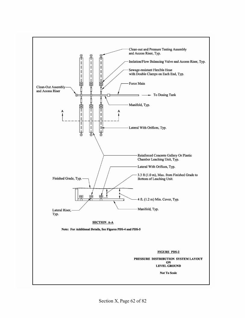
Section X, Page 62 of 82

Section X, Page 63 of 82

Section X, Page 64 of 82
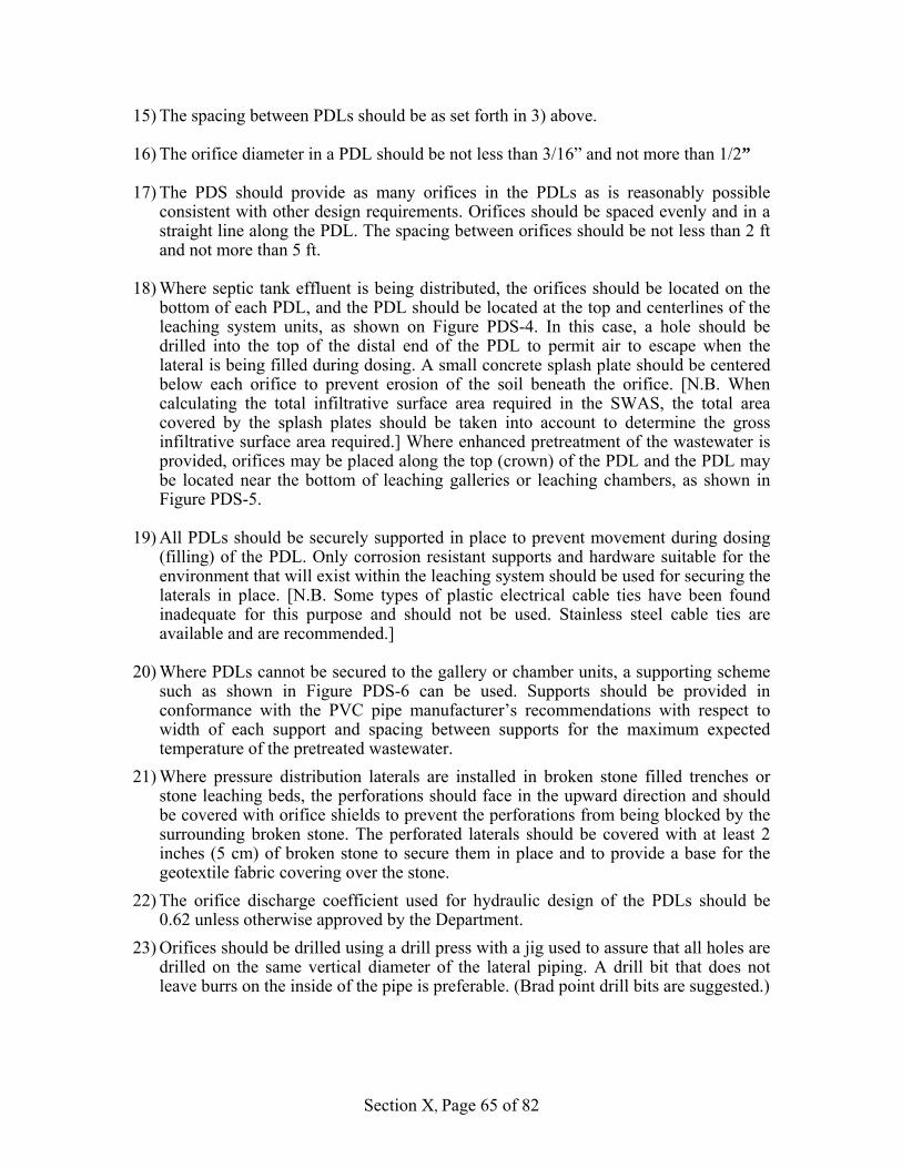
Section X, Page 65 of 82
15) The spacing between PDLs should be as set forth in 3) above. 16) The orifice diameter in a PDL should be not less than 3/16” and not more than 1/2” 17) The PDS should provide as many orifices in the PDLs as is reasonably possible
consistent with other design requirements. Orifices should be spaced evenly and in a straight line along the PDL. The spacing between orifices should be not less than 2 ft and not more than 5 ft.
18) Where septic tank effluent is being distributed, the orifices should be located on the
bottom of each PDL, and the PDL should be located at the top and centerlines of the leaching system units, as shown on Figure PDS-4. In this case, a hole should be drilled into the top of the distal end of the PDL to permit air to escape when the lateral is being filled during dosing. A small concrete splash plate should be centered below each orifice to prevent erosion of the soil beneath the orifice. [N.B. When calculating the total infiltrative surface area required in the SWAS, the total area covered by the splash plates should be taken into account to determine the gross infiltrative surface area required.] Where enhanced pretreatment of the wastewater is provided, orifices may be placed along the top (crown) of the PDL and the PDL may be located near the bottom of leaching galleries or leaching chambers, as shown in Figure PDS-5.
19) All PDLs should be securely supported in place to prevent movement during dosing
(filling) of the PDL. Only corrosion resistant supports and hardware suitable for the environment that will exist within the leaching system should be used for securing the laterals in place. [N.B. Some types of plastic electrical cable ties have been found inadequate for this purpose and should not be used. Stainless steel cable ties are available and are recommended.]
20) Where PDLs cannot be secured to the gallery or chamber units, a supporting scheme
such as shown in Figure PDS-6 can be used. Supports should be provided in conformance with the PVC pipe manufacturer’s recommendations with respect to width of each support and spacing between supports for the maximum expected temperature of the pretreated wastewater.
21) Where pressure distribution laterals are installed in broken stone filled trenches or stone leaching beds, the perforations should face in the upward direction and should be covered with orifice shields to prevent the perforations from being blocked by the surrounding broken stone. The perforated laterals should be covered with at least 2 inches (5 cm) of broken stone to secure them in place and to provide a base for the geotextile fabric covering over the stone.
22) The orifice discharge coefficient used for hydraulic design of the PDLs should be 0.62 unless otherwise approved by the Department.
23) Orifices should be drilled using a drill press with a jig used to assure that all holes are drilled on the same vertical diameter of the lateral piping. A drill bit that does not leave burrs on the inside of the pipe is preferable. (Brad point drill bits are suggested.)

Section X, Page 66 of 82

Section X, Page 67 of 82
Section X, Page 68 of 82

Section X, Page 69 of 82
24) Irrespective of what type of drill bit is used, any burrs on the inside and outside of the PDL piping, and any cuttings resulting from drilling of the orifices should be carefully removed without disturbing the drill holes (orifices). Removal of burrs on the inside of the PDL can be accomplished by pushing a pipe of a smaller diameter than the lateral through the pipe with the orifices oriented in the 6 O’clock (downward) position.
25) The PDLs should drain between doses, to prevent freezing. However, in order to minimize the drain-back volume, the force main and pressure distribution manifolds should be installed at a depth below the laterals, where freezing will not occur, and should not be designed to drain between doses. The minimum depth from finished ground surface to the top of the force main and pressure distribution manifolds should not be less than 4 feet (1.2 m). Refer to Figures PDS-4 and PDS-5.
26) Valves should be installed at the proximal (inlet) end of each PDL to permit balancing the flows to all the PDLs. These valves should be PVC True-Union type ball valves, plug valves, pinch valves, or other types of valves suitable for the service conditions to be encountered. Access risers, with frost proof frames and covers, or other means acceptable to the Department, should be installed to provide free access to these valves. Typical details for balancing valve installations are shown in Figures PDS-4 and PDS-5.
27) Provisions should be made for cleaning PDLs (flushing of sediment and unblocking clogged orifices), and to enable checking of operating pressures in the PDLs. These should consist of PVC sanitary tees installed at the proximal (near) end and distal (far) end of each PDL to facilitate cleaning the PDLs and also to provide for visual evidence of balanced flow, as described hereinafter. The branch of the tee should face vertically upwards and should be provided with a removable clean-out stub, as shown in Figures PDS-4 and PDS-5. The clean-out stub should be removable to insure that cleaning tools can enter directly into the sanitary tee if the stub interferes with access.
28) The sanitary tees, clean-out stub, and associated fittings should be of the same nominal diameter as the PDL. Access risers, with frost proof frames and covers or other freeze protection means should be installed to provide free access to the sanitary tee risers.
29) Provisions should be made for cleaning of manifolds. These should be similar to the
provisions made for cleaning of PDLs as described above and as shown in Figures PDS-4 and PDS-5.
30) During construction, the orifices, and ends of all PDLs, manifolds, and force mains
that have not been sealed with clean-out plugs, should be protected to keep rodents, insects, dirt and other debris out of the piping.
31) After construction has been completed, and before flow balancing is undertaken, the
flow balancing valves on each PDL should be closed and the plugs removed from the clean-out stubs at the ends of the pressure distribution manifold(s). The force main and pressure distribution manifold(s) should then be thoroughly flushed with clean water until all debris that may have entered the piping has been removed.
32) The flushing plugs should then be reinstalled at the ends of the pressure distribution
manifold(s)to affect a watertight closure.
Section X, Page 70 of 82
33) After the force main and pressure distribution manifold have been thoroughly flushed, the balancing valves at the proximal end of each PDL should be opened, beginning with the laterals at the proximal end of the distribution manifold. The threaded plug should then be removed from the top of the clean-out stub at the distal end of each PDL. The PDL should then be thoroughly flushed with clean water, after which the threaded plug should be replaced. This procedure should then be repeated for each PDL, proceeding in the direction toward the distal end of the manifold.
34) After the PDS has been flushed clean, it should be flow-balanced (calibrated) in the
following manner:
a. Remove the threaded plugs at the top of the clean-out stubs at the distal ends of PDLs connected at the same location along the manifold.
b. Connect clear PVC test standpipes, of the same diameter as the PDLs, with a thread x socket adapter cemented thereto, to the clean-out stubs. The height of each test standpipe should be such that the liquid in the standpipe should remain at least a few feet below the open top of the standpipe when the PDS is being dosed at the normal dose rate. Clean water may be used for calibration purposes.
c. During dosing, the observed static elevation of the liquid level in the clear
standpipes at the ends of the laterals being tested should be marked on the standpipes and recorded. A surveyor’s level should be used to determine the static elevations based on the project bench mark elevation.
The difference in liquid level elevations in the standpipes at the distal end of each pair of PDLs installed at the same elevation and being fed from the same location on the manifold should not exceed 4 in. Also, the average pressure head in any pair of PDLs should not differ by more than 6 in. from the average pressure head in any other pair of PDLs. If either of these tolerances is exceeded, the flow balancing valves should be adjusted until the liquid levels and pressure heads are within the stated tolerances. The pressure heads can be determined by measuring the distance from the liquid level in the standpipes to the top of the laterals. [N.B. When the PDS has been suitably flow balanced, the position of the valve handle should be marked on the top of the valve body for future reference in resetting the valve position should the valve setting be changed during cleaning or isolation of the PDLs.]
d. If the PDS cannot be adjusted to meet the liquid level elevation and pressure
tolerances given above, the PDS should be investigated by the Project Engineer to determine the reason for this discrepancy. The Project Engineer should then advise the Department of his findings, conclusions, and recommendations for any corrective actions that may need to be taken.
Section X, Page 71 of 82
The design of a PDS should be accomplished using detailed hydraulic calculations rather than using nomographs, curves or tables. These calculations can be performed manually, or by use of a computer spreadsheet program developed for this purpose, or by use of special computer programs developed for this purpose or that can be utilized (adapted) for this purpose.
Care should be taken in using computer programs to insure that the correct orifice coefficient (0.62) is used, as some computer programs may be based on discharge coefficients for flow control devices other than orifices. The design calculations for a PDS should be submitted to the Department for review along with documentation for any spreadsheet program or other computer program used in designing the system. The documentation should show the methodology used by the program [flow charts, algorithms, hydraulic formulas, spreadsheet formulas, etc.]. In the case of special computer programs, supporting information should also be submitted demonstrating that the program has been checked for various cases by manual calculations or by actual experiments conducted in the laboratory or in the field to substantiate the program results. 5. Design Methodology for Low Pressure Distribution Systems A methodology commonly used for design of a PDS is given below. Publications containing detailed information and procedures that may be found useful for design of a pressure distribution system are listed in the bibliography at the end of this section. • Select SWAS configuration. Determine the total length of leaching system galleries
or chambers required, based on the total infiltrative surface area required and the infiltrative surface area allowance per linear foot of leaching system used.
• The infiltrative surface area required will be based on the adjusted LTAR, which in
turn is based on the saturated hydraulic capacity of the soil and the wastewater strength, as discussed elsewhere in this document. [N.B. When calculating the total infiltrative surface area required in the SWAS, the total area covered by splash plates beneath downward facing orifices should be taken into account to determine the gross infiltrative surface area required.]
• Divide the total length of galleries or chambers required into equal length rows. The
length of a row, and the number of such rows, will depend upon the site-specific linear hydraulic loading rate that the soil will accept and convey away from the SWAS while still providing the required depth of unsaturated soil between the bottom of the SWAS and the mounded seasonal high ground water table.
• Determine the configuration of the PDS, including type of manifold. Chose the orifice
size and spacing. The orifice size and spacing should conform to the limits established herein and should not be any greater than necessary to meet the dosing requirements while insuring that essentially equal distribution will occur along the length of each lateral and between laterals. Shorter spacing between orifices will provide better utilization of the renovative capacity of the soil.

Section X, Page 72 of 82
• Chose the lateral diameter. The lateral diameter should be such that the difference in
pressures between the proximal orifice and the distal orifice should not exceed 10% of the operating pressure specified for the orifices.
• Select manifold size. The manifold diameter should be such that the difference in
pressure (the total head) between the proximal lateral-to-manifold connection and the distal lateral-to-manifold connection should not exceed 10% of the operating head required at the proximal orifice for each lateral.
• Optimize the PDS design. Repeat steps 1-5 until the PDS design is optimized with
respect to flow balancing, minimum dose volume, number of doses per day, and dosing pump capacity.
Pressure distribution systems installed on sloping terrain require special attention to insure that the PDS meets the requirements set forth above. It is left to the ingenuity of the designer to determine the best type of PDS to be used for a particular sloping site. In such cases, it may be necessary to use more than one configuration of a PDS, or to vary the pipe diameters, orifice diameters and/or orifice spacing for individual PDLs, in order to obtain the equal distribution desired. [N.B. Care should be taken if orifice diameters and/or spacing change within the same PDS, as this can lead to errors in construction of the PDS, due to installing a PDL in the wrong location.] Consideration should also be given to using stainless steel orifice plates inserted in unions to provide equal distribution of flow into the PDLs at their various elevations in the PDS. It may also be necessary to utilize more pumps than are required for a PDS situated on level ground, with different pumps being dedicated to each part of the SWAS that lies at an elevation different from that of the other portions. 6. Maintenance of Pressure Distribution Systems PDLs should be inspected and flushed periodically to ensure proper distribution. This should be done at least once per year. Inspection should include checking the residual pressure at the distal ends of the laterals and comparing the results with the results initially obtained when the PDS was flow balanced. When the results indicate the residual pressure exceeds 130% of the initial value, the PDLs should be cleaned to unclog the orifices. An initial indication of clogged orifices may be a significant increase in the running times of the dosing pumps, but experience has indicated that increases in residual pressure are a more sensitive indication of clogging as compared to pump running time. Flushing of the PDLs can be accomplished by using the cleanouts provided at the distal end of each lateral. Flushing may be accomplished by use of the pretreated effluent and the pumps in the dosing tank. Provisions should be made for capturing the flushing water and discharging it to a septic tank pumper truck. Periodically, the manifold should be flushed to remove any sediment accumulations, using the cleanout provided at the distal end of the manifold. Flushing may be accomplished by use of the pretreated effluent and the pumps in the dosing tank. Provisions should be made for capturing the flushing water and discharging it to a septic tank pumper truck, or flow equalization tank, if provided, or to the second compartment of the septic tank. In the latter case, the discharge rate should be such as will not unduly disturb the operation of the septic tank.

Section X, Page 73 of 82
Unclogging of the orifices can be accomplished by using a plumber’s snake equipped with a bristle brush head, or by a water jet device used for such purposes, or by other suitable methods, using the cleanouts provided at each end of the lateral. The residual pressure at the distal end should then be rechecked to ensure it has dropped to its initial value. J. Recommended Types of Subsurface Wastewater Absorption Systems
1. Rows of Stone filled Trenches 2. Rows of Precast Reinforced Concrete Shallow Galleries. 3. Rows of Factory Manufactured Plastic Chambers. 4. Beds composed of stone filled beds, rows of Shallow Concrete Galleries or Plastic
Chambers, but only when enhanced pretreatment of the wastewater is provided. 5. Systems using other types of leaching units that have been approved by the
Department.
Note: Enhanced pretreatment is defined as that which will provide an effluent having mean BOD5 and TSS concentrations ≤ 30 mg/L respectively. Where enhanced pretreatment for nitrogen removal is required, the effluent should have a mean BOD5 concentration ≤ 15 mg/L.
Concrete galleries and plastic chambers should be designed and constructed to support the load of the overburden soil and the vehicular wheel loads that can be expected to be imposed upon these units. For long-term durability, concrete galleries should be constructed using a concrete mixture that will have a 28-day compressive strength of not less than 4,000 pounds per sq. in.
K. Maximum Distance from Ground Surface to Bottom of SWAS
1. It is desirable to minimize the distance from the finished ground surface to the bottom of the SWAS in order to provide the shortest path for diffusion of air into the unsaturated zone beneath the SWAS. Many studies have shown that aerobic conditions in this zone are required in order to provide adequate renovation of the wastewater. Therefore, it is preferable to use shallower-depth trenches, galleries and chambers.
2. A reasonable goal is to keep the vertical distance from finished grade (the ground surface that will exist after construction of the SWAS is completed) to the bottom of the SWAS at 3.3 ft or less. This distance should not be exceeded unless satisfactory provisions are made for introduction of oxygen to the unsaturated zone beneath the SWAS.

Section X, Page 74 of 82
L. Surfaces over SWAS
1. No roadway, driveway, parking area, turning area or other area surfaced so as to be considered impervious should be located above a SWAS unless otherwise approved by the Department. Where a SWAS is permitted to be located beneath an impervious surface, it should be provided with an air delivery system to provide a means of introducing atmospheric oxygen into the unsaturated zone beneath the SWAS.
2. Where ventilation piping is provided, it should terminate in an air intake riser with
a U-bend, with terminal end of bend at least 30” above finished grade. The intakes should be covered with corrosion resistant screening to prevent entry of vermin and other small animals. The intake risers should be located where they are not susceptible to damage.
M. Enhanced Pretreatment SWAS
When highly pretreated wastewater (BOD5 and TSS ≤ 30 mg/L respectively) will be discharged to a SWAS, the system may consist of beds, as described below.
1. Precast concrete galleries or plastic leaching chambers, with 24 inches of broken
stone placed between adjacent rows of galleries or chambers, 3 inches of broken stone beneath the galleries or chambers, and 12 inches of broken stone placed along the outside sidewall areas of the outer rows of galleries or chambers.
2. Rows of galleries or chambers placed side by side, with no broken stone on the
bottom, and 12 inches of stone on the outside sidewall areas of the bed. Where chambers are used, broken stone should be placed in the areas between the adjacent chamber walls, to the full height of the chambers.
3. Beds of broken stone at least 12 inches in depth below the PDLs. The PDLs
should be placed in parallel lines not more than 6 feet apart. 4. The maximum LTAR for highly pretreated wastewater should be 1.2 gpd/sf of
bottom area or 5% of the vertical saturated hydraulic conductivity, whichever is less.
N. Broken Stone and Screened Gravel Aggregate
1. Aggregate used for construction of an SWAS should consist of washed broken stone or washed screened gravel conforming to the gradation given in Table J-1.

Section X, Page 75 of 82
TABLE J-1
Gradation Requirements for Broken Stone and Screened Gravel Aggregate
U.S.A. Standard Series Sieves, ASTM E-11 mm Sieve No*. Percent Passing 50 2 100 38.1 11/2 90-100 25 1 20-55 19 3/4 0-10 9.5 3/8 0-5 0.425 40 0-2 0.075 200 0-1 2. Aggregate should consist of sound, tough, durable stone or gravel, free from
silt, dirt, soft, thin, elongated, friable, laminated, micaceous or disintegrated pieces, meeting the following requirements:
a. Soundness: When tested with magnesium sulfate solution for soundness
using AASHTO Method T 104, the aggregate should not have a loss of more than 10% at the end of five cycles.
b. Hardness: >3 on Moh’s hardness scale. (Note: Aggregate that will not
leave residue of aggregate material when used to scratch a copper penny, or the penny will not scratch the aggregate, will meet this requirement.)
3. No aggregate fill should be placed on the bottom area of the SWAS within the
limits of the inside bottom dimensions of the galleries or chambers, unless the wastewater has received enhanced pretreatment.
O. Horizontal Layout of Trench, Gallery and Chamber Rows
1. All trench, gallery and chamber rows should generally follow ground contours.
2. Where septic tank effluent is discharged to an SWAS, the minimum center to center distance between individual trench, gallery or chamber rows should not be less than 3 times the outside width of the trench, gallery or chamber row.
3. The maximum length of individual gallery and chamber rows should be based on the length of the pressure distribution system perforated pipe laterals determined as set forth elsewhere in this document.
P. Vertical Alignment of Individual Gallery and Chamber Rows
The bottoms of gallery and chamber rows fed by pressure distribution laterals extending from the essentially the same location on a pressure distribution manifold should be at the same elevation and level throughout their length.
Section X, Page 76 of 82
Q. Systems in Flood Plains On-site wastewater renovation systems (OWRS) installed in designated flood plains, or other areas subject to flooding (herein considered as undesignated flood plains), should conform to the following requirements, unless any local regulatory agency or Federal Emergency Management Agency(FEMA) requirements are more stringent, in which case those local or Federal requirements should govern.
1. No fill should be placed in a flood plain for construction of an OWRS, including
access ways to the OWRS, unless specific approval for such fill is obtained from those regulatory agencies having jurisdiction over placement of fill in flood plains.
2. An OWRS located in a flood plain should be located on the highest feasible
naturally occurring area of the project site and should have preference in location over all other improvements except the water supply well.
3. The minimum bottom elevation of a subsurface wastewater absorption system
(SWAS) should be no lower in elevation than one foot above the elevation of the “10 year” still water level designated by FEMA for the area in which the SWAS will be located.
4. Tops of grease traps and septic tanks installed in flood plains should be no lower
in elevation than two feet above the elevation of the “10” year flood still water level, and risers should be provided with watertight covers.
5. Pretreatment facilities (excluding septic tanks), control buildings, pump
chambers, and emergency electrical generation equipment and their mechanical and electrical components should be located above the 100 year flood still water level designated by FEMA or protected from such floods by methods approved by the Department.
6. In Coastal areas subject to high-velocity wave action (V zones as defined by
FEMA), and in floodway and floodway fringe areas in A zones (as defined by FEMA) subject to soil erosion by flowing water, all above-ground structures should be designed and anchored to prevent floatation, collapse, and lateral movement resulting from hydrodynamic and hydrostatic loads, including the affects of buoyancy. All underground tanks, including but not limited to fuel tanks, grease traps, septic tanks, equalization tanks, other pretreatment process tanks, valve chambers, and pump chambers, should be protected from damage due to erosion by wave action and flood water velocity and anchored to prevent floatation, and should be provided with watertight access covers.
7. In flood plains, the surfaces of walkways and drives that provide access to
pretreatment facilities (excluding grease traps and septic tanks), control buildings, pump chambers, and emergency electrical generation equipment and their mechanical and electrical components should be no lower in elevation than one foot above the “10 year” flood still water level.

Section X, Page 77 of 82
8. As soon as a flooding event is over, and the water levels have receded to the point where the on-site system can be inspected, any damage to the system and the adjacent ground should be reported to the Department and repaired to the satisfaction of the Department. Particular attention should be paid to inspecting and cleaning any grease trap and septic tank effluent filters.
R. Construction of Subsurface Wastewater Absorption Systems
1. Construction of a SWAS should not be undertaken when the ground is frozen or when the ambient temperature is below freezing, or during and immediately following a precipitation event.
2. The initial and any reserve areas set aside for the SWAS, as well as the area
immediately down-gradient of the system, should be protected as much as possible from compaction by the contractor’s equipment. The use of rubber-tired equipment such as trucks, compactors, backhoes, bucket loaders, etc. should be restricted in these areas. In sandy soils, where such compaction may only be moderate, significant reductions in the soil hydraulic conductivity may occur. In loamy soils, (particularly in silt and clay loams) such compaction can reduce the hydraulic conductivity by orders of magnitude and result in a system failure. Therefore, use of tracked equipment is preferable to wheeled equipment, as the former will exert much less compactive force on the soil.
3. Care should be taken to avoid, as much as possible, the clogging of infiltrative
surfaces during construction by smearing with the excavation equipment. If such surfaces are smeared, they should be properly scarified to remove the smeared soils. Loose materials caused by scarification should be removed from the area of the SWAS.
4. Proper materials should be used for construction of the system and careful
attention should be paid to the various elevations and grades required for the infiltration surfaces and installation of the various pipes and leaching units.
5. Excavated material should be placed sufficiently distant from the area in which
the SWAS is to be constructed so that it cannot be washed into the excavated area during precipitation events. The excavated material should be placed up-gradient of the SWAS and not in the down-gradient area between the SWAS and the nearest point of concern, to avoid changing the hydraulic carrying capacity of the soil by compaction. In some cases, it may be necessary to install a silt fence or hay bales between the piles of excavated material and the area(s) of the SWAS to avoid siltation of such area(s).
6. Where stone-filled trenches, galleries or chambers are to be installed in fill, the
fill should be placed to the full design height before excavating for installation of the trenches, galleries or chambers. Fill material should be placed by dumping around the edge of the SWAS area, keeping rubber tired vehicles and equipment off the area. Track-mounted equipment should be used to move the fill material into place.

Section X, Page 78 of 82
7. The bottom of the areas excavated for installation of leaching units should be checked to insure that it conforms to the lines and grades shown on the approved construction drawings, and any deviations found should be corrected.
8. Where additional fill is required to bring the bottom of the excavation to grade, it
should conform to and be placed in accordance with the construction specifications approved by the Department and as specified elsewhere in this document. When the bottom elevation of the excavation is satisfactory and adequately compacted, it should be raked with a garden or landscape rake to a depth of at least one inch before placement of stone, galleries, or chambers, or pressure distribution piping.
9. After the leaching facilities and associated effluent distribution systems are
installed, the top of aggregate fill should be protected by a durable geotextile fabric.
10. The fabric should be listed on the Connecticut Department of Transportation’s
Approved Products List for geotextile - Subsurface Drainage, Class A, and should be of the non-woven type.
11. Where an SWAS is installed in a fill system, the fabric should extend horizontally
to at least 1 ft beyond the top edge of the aggregate fill in each lateral direction. Where an SWAS is installed in original ground, the fabric should extend vertically upwards along the sides of the trench at least 6 inches.
12. Geotextile fabric should also be placed over each joint of leaching units, with at
least 6 inches of overlap on each side of the joint, and should extend horizontally or vertically as indicated above for fabric over the top of aggregate fill.
13. Backfill should be carefully placed and over-compaction of this material should
be avoided. The top six (6) inches (15 cm) of earth cover material placed over the SWAS should be suitable for establishing a healthy turf.
14. The ground surface over the entire SWAS should be graded and maintained to
divert surface water away from the top of the system. The SWAS should be protected from siltation or erosion during and after construction.
15. All of the areas disturbed by construction, not otherwise scheduled to be surfaced,
should be limed, fertilized, seeded and mulched so as to establish a healthy turf.
16. Grassed areas in and around SWAS should be moved at least three times during the growing season.

Section X, Page 79 of 82
S. References Amerson, R.S., E.J. Tyler, and J.C. Converse. 1991. Infiltration as Affected by
Compaction, Fines and Contact Area of Gravel. In: Onsite Wastewater Treatment, Proc. of the 6th National Symposium on Individual and Small Community Sewage Systems. ASAE., St. Joseph, MI. pp. 243-247.
Anderson, J. L., R.E. Machmeier, and M.J. Hansel. 1981. Long-Term Acceptance Rates
of Soils for Wastewater. In: Proceedings of the Third National Symposium on Individual and Small Community Sewage Treatment. ASAE, Chicago, Illinois. December 1981: pp. 93-100.
Anderson, D.L, A.L. Lewis, and K.M. Sherman. 1991. Human Enterovirus Monitoring at
Onsite Sewage Disposal Systems in Florida. In Proceedings of the Sixth National Symposium on Individual and Small Community Sewage Systems. American Society of Agricultural Engineers St. Joseph, Michigan December 1991.
Bouma, J. and F.R. Magdoff. 1974. The Development of Soil Clogging in Sands
Leached with Septic Tank Effluent. In: 1974 Proc. ASAE St. Joseph, MI pp. Burks, B.D. and M.M. Minnis. 1994 Onsite Wastewater Treatment Systems. Hogarth
House, LTD. Madison, WI. Chapter 5 - Hydraulics. pp. 99-112 Crosby, J.W., D.L. Johnstone, C.H. Drake and R.L. Fenton. 1968. Migration Of
Pollutants In Glacial Outwash Environment. Water Resources Res. V.4, pp. 1095-1115.
Domenico, P.A. and G. A. Robbins 1995. A New Method of Contaminant Plume
Analysis. Ground Water, V. 23, No 4. July-Aug. 1985. Domenico, P.A. and F.W. Schwartz 1990. Physical and Chemical Hydrogeology. John
Wiley & Sons. New York, NY. July 1990. Erlsten, S. and D. Bloomquist. 2001. Long Term Acceptance Rates of Common Floridian
Soils. Departments of Environmental Engineering Sciences and Civil & Coastal Engineering. Univ. of Florida. Gainsville, FL.
Freeze, R.A. and J.A. Cherry 1979. Groundwater. Prentice-Hall, Inc. Englewood Cliffs, NJ Graetz, D.A. and V.D. Nair. 2000. Phosphorus Sorption Isotherm Determination. In:
Methods of Phosphorus Analysis for Soils, Sediments, Residuals, and Waters. Southern Cooperative Series Bulletin No. 396. G. M. Pierzynski, Ed. Department of Agronomy, Kansas State Univ. Manhattan, KS.
Healy, K.A. and R. Laak. 1974. Site Evaluation and Design of Seepage Fields. Jour.
Environ. Eng. Div. ASCE. V. 100. EE5: pp 1133-1146.

Section X, Page 80 of 82
S. References, Continued Healy, K.A. and R. May 1982 Seepage and Pollutant Renovation - Analysis for Land
Treatment, Sewage Disposal Systems (Rev. 1997). CT. Department of Environmental Protection. Hartford, CT.
Higgins, J., G. Heufelder and S. Foss. 2000. Removal of MS2 Coliphage by Standard
Septic Tank-Leach Trench Septic Systems. MA. Dept. of Environmental Protection Training Center. Millbury, MA.
Hoxie, D.C. and A. Frick. 1984. Subsurface Wastewater Disposal Systems Designed in
Maine by the Site Evaluation Method. Life Expectancy, System Design and Land Use Trends. In: Proc. of the Fourth National Symposium on Individual and Small Community Sewage Systems. ASAE. St. Joseph, MI. pp 362-371
Jacobson, N.L. 2001. Nutrient Reduction - Nitrogen. CT DEP. Hartford, CT. Jacobson, N.L. 2002. Analysis of Vertical Separating Distance Between Septic Tank Leaching
Systems and Ground Water. Report to the Connecticut Department of Environmental Protection. Hartford, CT., November 2002
Jensen, P. D., and R.L. Siegrist. 1991. Integrated Loading Rate Determination for
Wastewater Infiltration System Sizing. In: Proceedings of the Sixth National Symposium on Individual and Small Community Sewage Systems. ASAE. Chicago, IL. Dec. 1991. pp. 183-191.
Laak, R. 1966 The Effect of Aerobic and Anaerobic Household Sewage Pretreatment
on Seepage Beds. Ph.D. Thesis, University of Toronto, Canada. Laak, R. 1970. Influence of Domestic Wastewater Pretreatment on Soil Clogging.
Journal WPCF, Vol. 42, No. 8, Part 1, August 1970: pp. 1495-1500. Laak, R. 1977. Septic Tank and Leaching Field Operation, Problems and Renovation.
Section 2. Clogging Consideration. Presented at: Wastewater Treatment Systems for Private Homes and Small Communities. Central New York Regional Planning and Development Board. Syracuse, NY. June 22-23, 1977.
Loudon, T. L., G.S. Salthouse, and D.L. Mokma. 1998. Wastewater Quality and Trench
System Design Effects on Soil Acceptance Rates. In: Proceedings of the Eight National Symposium on Individual and Small Community Sewage Systems. ASAE. Orlando, Fl., March 1998. pp. 186-194.
Loudon, T. L. and D.L. Mokma. 1999. Trench Infiltration as Influenced by Soil Type,
Depth, Application Method and Effluent Quality. In: Proceedings 10th Northwest On-Site Wastewater Treatment Short Course and Equipment Exhibition. University of Washington. Seattle, WA. pp. 341-352.

Section X, Page 81 of 82
S. References, Continued Matejcek, B.C., S. Erlsten, and D. Bloomquist. 2000. Determination of Properties and
the Long Term Acceptance Rates of Effluents from Food Service Establishments that Employ Onsite Sewage Treatment. Departments of Environmental Engineering Sciences and Civil & Coastal Engineering. Univ. of Florida. Gainsville, FL. 167 pgs.
Mooers, J.D. and D.H. Waller 1996. Vertical Separation and Groundwater Mounding
Beneath Septic Systems-Appendix 1: Mound Calculation Program. In: On-Site Wastewater Research Program – Final Report, Phase III 1994-1996. Report to Province of Nova Scotia. Center for Water Resources Study, Technical University of Nova Scotia.
Otis, R.J. 1984. In: Proc. Fourth National Symposium on Individual and Small
Community Sewage Systems. December 10-11, 1984 New Orleans, LA. ASAE. St. Joseph, MI. pp. 238-249.
Pask, D.A. 1988. Hydrogeological Aspects of On-Site Sewage Disposal into Surficial
Soils in Nova Scotia. Nova Scotia Department of Health. Halifax, N.S. Canada.
Pask, D. 1994. Lateral Thinking in Ground Water Flow: Introducing Contour Disposal
Fields. Small flows, V. 8, No. 1 Winter 1994. NSFC, West Virginia U. Morgantown, WV.
Reneau, R. B., Jr. 1979. Changes in concentrations of selected chemical pollutants in wet,
tile-drained soil systems as influenced by disposal of septic tank effluents. J. Environ. Qual., V 8, pp 189-196.
Siegrist, R. L., D. L. Anderson, and J.C. Converse. 1984a. On-Site Treatment and
Disposal of Restaurant Wastewater. Small Scale Management Project, Univ. of Wisconsin-Madison. Madison, WI.
Siegrist, R. L., D. L. Anderson, and J.C. Converse. 1984b. Commercial Wastewater On-
Site Treatment and Disposal. In: Proc. of Fourth National Symposium on Individual and Small Community Sewage Systems. ASAE, St. Joseph, MI. pp. 210-219.
Siegrist, R. L. 1987a. Hydraulic Loading Rates for Soil Absorption Systems Based On
Wastewater Quality. In: Proceedings of the Fifth National Symposium on Individual and Small Community Sewage Systems, Chicago, IL. December 1987. pp. 232-241.
Siegrist, R. L., 1987b. Soil Clogging During Subsurface Wastewater Infiltration as
Affected by Effluent Composition and Loading Rate. J. Environ. Qual., V. 16, No. 2, 1987. pp. 181-187.

Section X, Page 82 of 82
S. References, Continued Siegrist, R. L., and S. Van Cuyk. 2001. Wastewater Soil Absorption Systems: The
Performance Effects of Process and Environmental Conditions. In: Proceedings of the Ninth National Symposium on Individual and Small Community Sewage Systems. Fort Worth, TX. March 2001. ASAE. St. Joseph, MI. pp 41-51.
Siegrist, R.L., J.E. McCray, and K.S. Lowe. 2004. Wastewater Infiltration into Soil and
the effects of Infiltrative Surface Architecture. Small Flows Quarterly, V. 5, No. 1. NSFC, West Virginia U. Morgantown, WV.
Tyler, E. J. and J.C. Converse 1989. Hydraulic Loading Based Upon Wastewater
Effluent Quality. Proceedings 6th Northwest On-Site Wastewater Treatment Short Course, University of Washington, Seattle, WA. September 1989: pp. 163-172.
Tyler, E. J. and J.C. Converse 1994. Soil Acceptance of Onsite Wastewater as Affected
by Soil Morphology and Wastewater Quality. In: Proceedings of the Seventh International Symposium on Individual and Small Community Sewage Systems. ASAE. Atlanta, GA. December 1994. pp. 185-194.
Tyler, E. J. 2001. Hydraulic Wastewater Loading Rates To Soil. In: Proceedings of the
Ninth National Symposium on Individual and Small Community Sewage Systems. ASAE. Fort Worth, TX. March 2001. pp. 80-86.
U.S.D.A. (1986). U. S. Department of Agriculture, Soil Conservation Service 1986.
Technical Release 55 (TR 55). 2nd Ed. Urban Hydrology for Small Watersheds.
U.S. Department of the Interior, Bureau of Reclamation. 1977. Design of Small Dams
U.S. Gov. Printing Office. Washington, DC White, K.D., and L. T. West. 2003. In Ground Dispersal of Wastewater Effluent: The
Science of Getting Water into the Ground. Small Flows Quarterly, V. 4, No. 2, pp. 28-35. NSFC, West Virginia U. Morgantown, WV.
Yates, M.V. and S.R. Yates. 1987. A Comparison Of Geo-Statistical Methods For
Estimating Virus Inactivation Rates In Ground Water. Wat. Res. V. 21, pp. 1119-1125.