Section 3.1-1 Copyright © 2014, 2012, 2010 Pearson Education, Inc. Lecture Slides Elementary...

Section 3.1-1Copyright © 2014, 2012, 2010 Pearson Education, Inc.

Lecture Slides

Elementary Statistics Twelfth Edition

and the Triola Statistics Series

by Mario F. Triola


Chapter 3Statistics for Describing,

Exploring, and Comparing Data

3-1 Review and Preview

3-2 Measures of Center

3-3 Measures of Variation

3-4 Measures of Relative Standing and Boxplots


Chapter 1Distinguish between population and sample, parameter and statistic, good sampling methods: simple random sample, stratified sample, etc.

Chapter 2Frequency distributions, summarizing data with graphs, describing the center, variation, distribution, outliers, and changing characteristics over time in a data set

Review


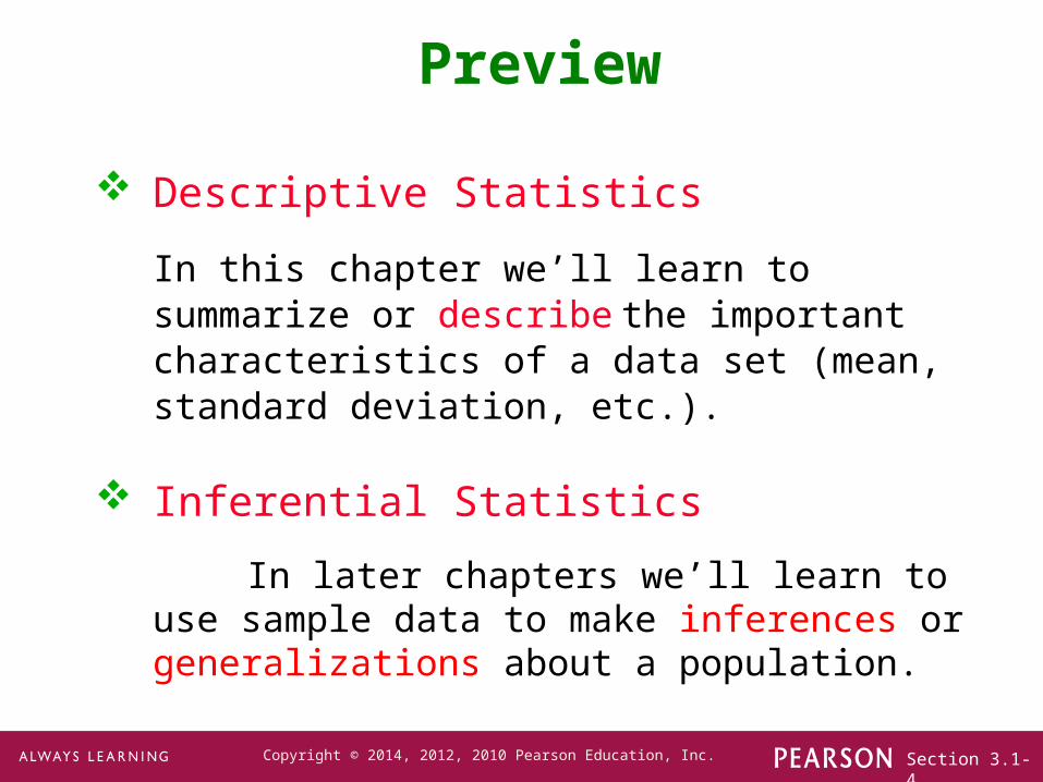
Descriptive Statistics

In this chapter we’ll learn to summarize or describe the important characteristics of a data set (mean, standard deviation, etc.).

Inferential Statistics

In later chapters we’ll learn to use sample data to make inferences or generalizations about a population.

Preview


Key Concept

Characteristics of center of a data set.

Measures of center, including mean and median, as tools for analyzing data.

Not only determine the value of each measure of center, but also interpret those values.


Basics Concepts of Measures of Center

Measure of Center

the value at the center or middle of a data set

Part 1


Arithmetic Mean

Arithmetic Mean (Mean)the measure of center obtained by adding the values and dividing the total by the number of values

What most people call an average.


Notation

denotes the sum of a set of values.

is the variable usually used to represent the individual data values.

represents the number of data values in a sample.

represents the number of data values in a population.

x

n

N


x

x

N

xx

n

Notation

is pronounced ‘mu’ and denotes the mean of all values in a population

is pronounced ‘x-bar’ and denotes the mean of a set of sample values


Advantages

Sample means drawn from the same population tend to vary less than other measures of center

Takes every data value into account

Mean

Disadvantage

Is sensitive to every data value, one extreme value can affect it dramatically; is not a resistant measure of center


Table 3-1 includes counts of chocolate chips in different cookies. Find the mean of the first five counts for Chips Ahoy regular cookies: 22 chips, 22 chips, 26 chips, 24 chips, and 23 chips.

Example 1 - Mean

SolutionFirst add the data values, then divide by the number of data values.

x x

n2222262423

5117

5 23.4 chips


often denoted by (pronounced ‘x-tilde’)

Median

Medianthe middle value when the original data values are arranged in order of increasing (or decreasing) magnitude

is not affected by an extreme value - is a resistant measure of the center

x


Finding the Median

1. If the number of data values is odd, the median is the number located in the exact middle of the list.

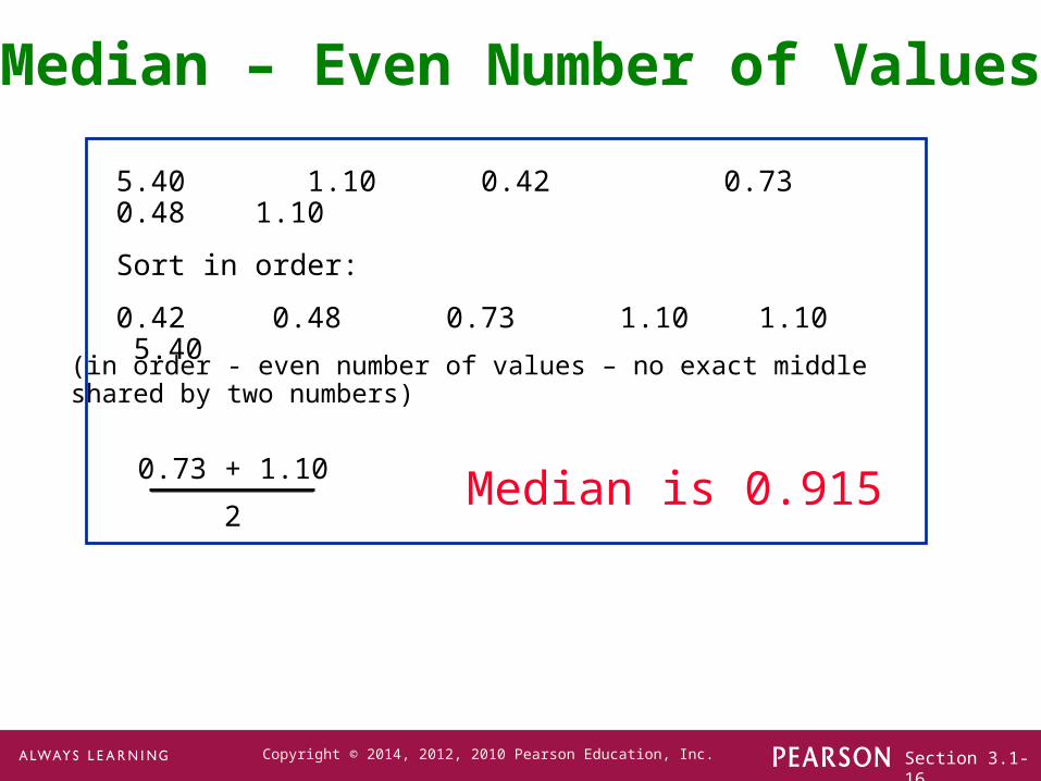
2. If the number of data values is even, the median is found by computing the mean of the two middle numbers.

First sort the values (arrange them in order). Then –


5.40 1.10 0.42 0.73 0.48 1.10 0.66

Sort in order:

0.42 0.48 0.66 0.73 1.10 1.10 5.40

(in order - odd number of values)

Median is 0.73

Median – Odd Number of Values


5.40 1.10 0.42 0.73 0.48 1.10

Sort in order:

0.42 0.48 0.73 1.10 1.10 5.40

0.73 + 1.10

2

(in order - even number of values – no exact middleshared by two numbers)

Median is 0.915

Median – Even Number of Values


Mode Mode

the value that occurs with the greatest frequency

Data set can have one, more than one, or no mode

Mode is the only measure of central tendency that can be used with nominal data.

Bimodal two data values occur with the same greatest frequency

Multimodal more than two data values occur with the same greatest frequency

No Mode no data value is repeated


a. 5.40 1.10 0.42 0.73 0.48 1.10

b. 27 27 27 55 55 55 88 88 99

c. 1 2 3 6 7 8 9 10

Mode - Examples

Mode is 1.10

No

Mode

Bimodal - 27 & 55


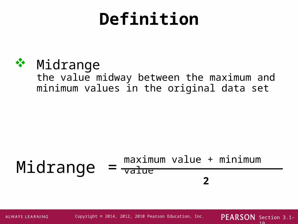
Midrangethe value midway between the maximum and minimum values in the original data set

Definition

Midrange = maximum value + minimum value

2


Sensitive to extremesbecause it uses only the maximum and minimum values, it is rarely used

Midrange

Redeeming Features

(1) very easy to compute

(2) reinforces that there are several ways to define the center

(3) avoid confusion with median by defining the midrange along with the median


Carry one more decimal place than is present in the original set of values

Round-off Rule for Measures of Center


Think about the method used to collect the sample data.

Critical Thinking

Think about whether the results are reasonable.


Example

Identify the reason why the mean and median would not be meaningful statistics.

a.Rank (by sales) of selected statistics textbooks: 1, 4, 3, 2, 15

b. Numbers on the jerseys of the starting offense for the New Orleans Saints when they last won the Super Bowl: 12, 74, 77, 76, 73, 78, 88, 19, 9, 23, 25


Beyond the Basics of Measures of Center

Part 2


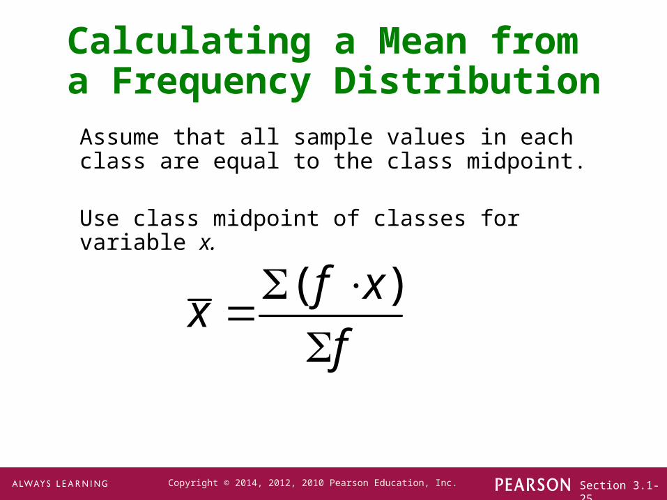
Assume that all sample values in each class are equal to the class midpoint.

Use class midpoint of classes for variable x.

Calculating a Mean from a Frequency Distribution

( )f xx

f


Example• Estimate the mean from the IQ scores in Chapter 2.

( ) 7201.092.3

78

f xx

f


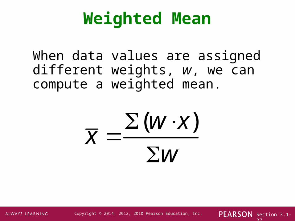
Weighted Mean

When data values are assigned different weights, w, we can compute a weighted mean.

( )w xx

w


In her first semester of college, a student of the author took five courses.

Her final grades along with the number of credits for each course were A

(3 credits), A (4 credits), B (3 credits), C (3 credits), and F (1 credit).

The grading system assigns quality points to letter grades as follows:

A = 4; B = 3; C = 2; D = 1; F = 0.

Compute her grade point average.

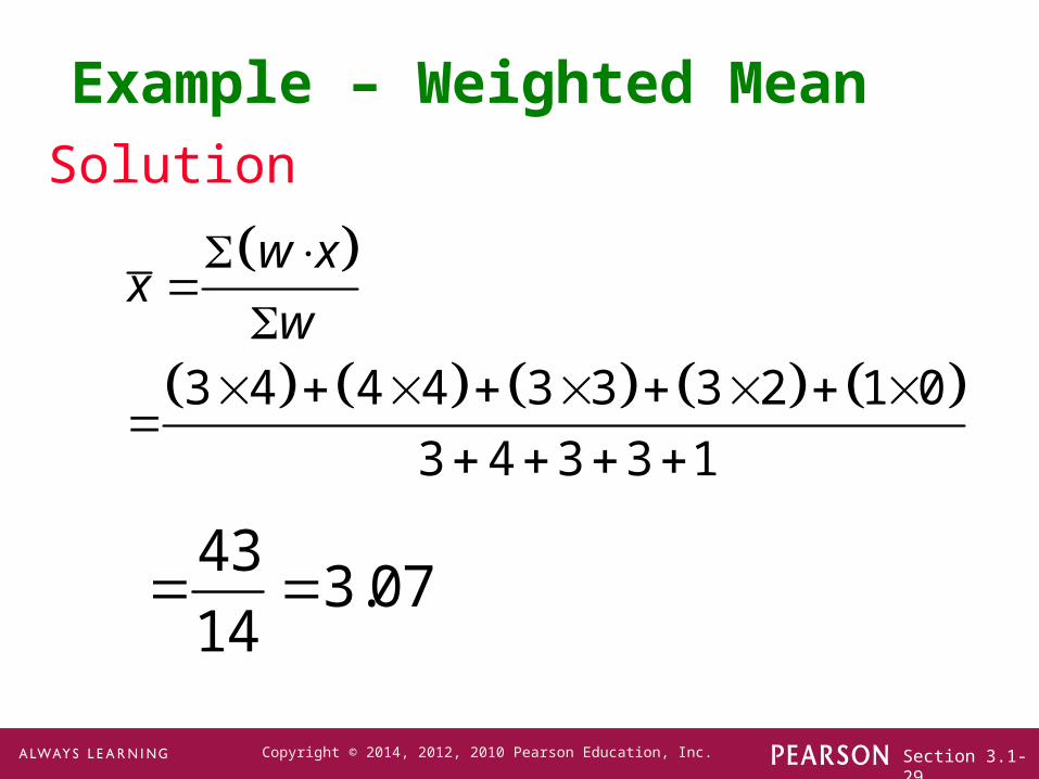
Example – Weighted Mean

SolutionUse the numbers of credits as the weights: w = 3, 4, 3, 3, 1.

Replace the letters grades of A, A, B, C, and F with the corresponding quality points: x = 4, 4, 3, 2, 0.


Solution

Example – Weighted Mean

3 4 4 4 3 3 3 2 1 0

3 4 3 3 1

w xx

w

.43

3 0714


Key Concept

Discuss characteristics of variation, in particular, measures of variation, such as standard deviation, for analyzing data.

Make understanding and interpreting the standard deviation a priority.


Basics Concepts of Variation

Part 1


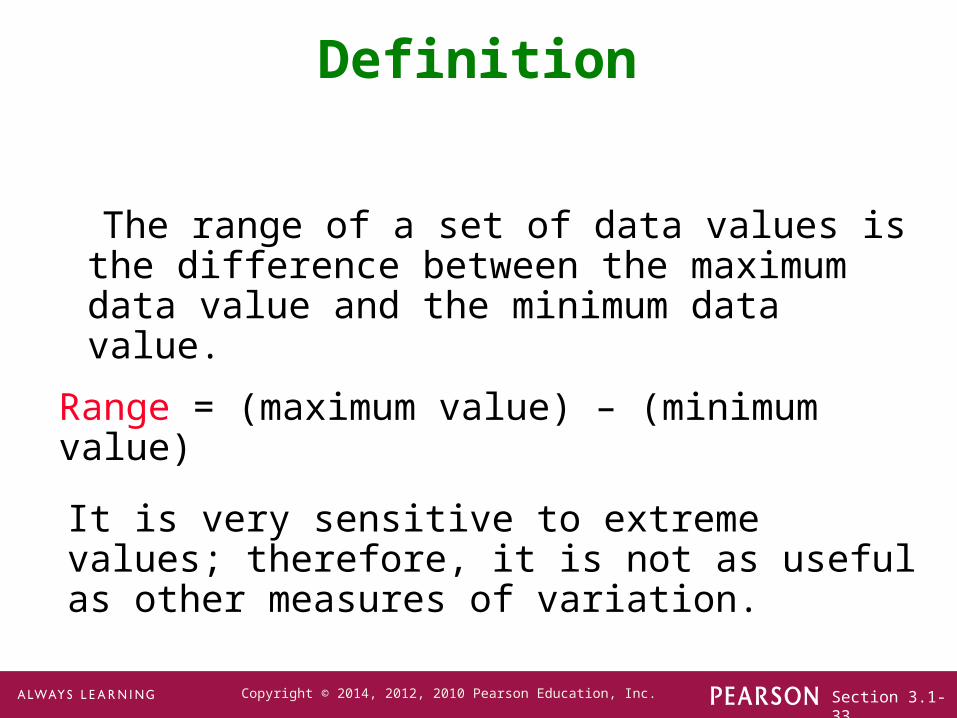
Definition

The range of a set of data values is the difference between the maximum data value and the minimum data value.

Range = (maximum value) – (minimum value)

It is very sensitive to extreme values; therefore, it is not as useful as other measures of variation.


Round-Off Rule for Measures of Variation

When rounding the value of a measure of variation, carry one more decimal place than is present in the original set of data.

Round only the final answer, not values in the middle of a calculation.


Definition

The standard deviation of a set of sample values, denoted by s, is a measure of how much data values deviate away from the mean.


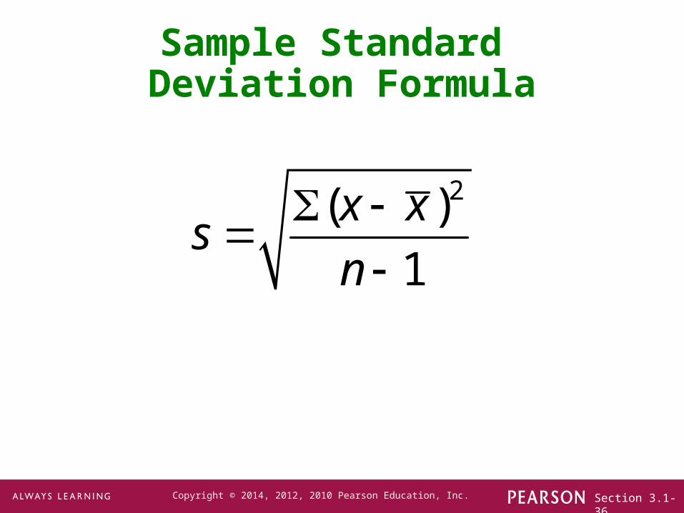
Sample Standard Deviation Formula

2( )

1

x xs

n


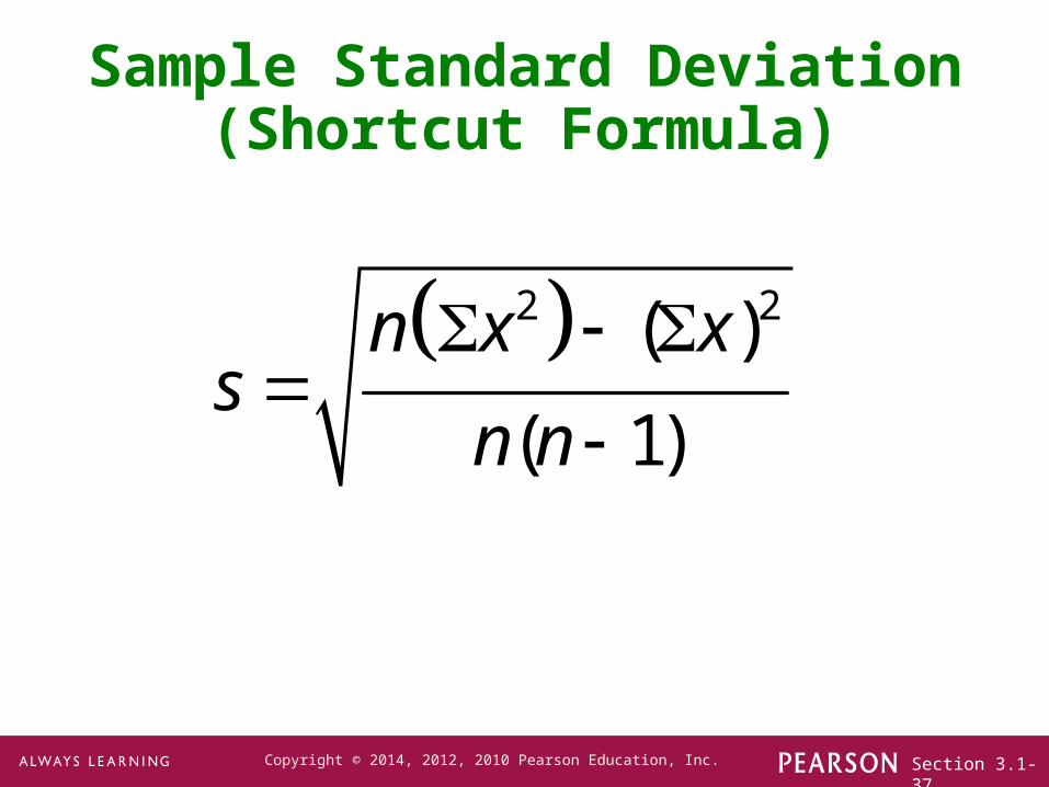
Sample Standard Deviation (Shortcut Formula)

2 2( )

( 1)

n x xs

n n


Standard Deviation – Important Properties

The standard deviation is a measure of variation of all values from the mean.

The value of the standard deviation s is usually positive (it is never negative).

The value of the standard deviation s can increase dramatically with the inclusion of one or more outliers (data values far away from all others).

The units of the standard deviation s are the same as the units of the original data values.


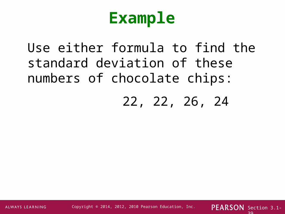
Example

Use either formula to find the standard deviation of these numbers of chocolate chips:

22, 22, 26, 24


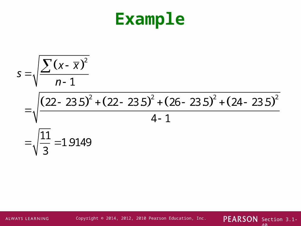
Example

2

2 2 2 2

1

22 23.5 22 23.5 26 23.5 24 23.5

4 1

111.9149

3

x xs

n


Range Rule of Thumb for Understanding Standard Deviation

It is based on the principle that for many data sets, the vast majority (such as 95%) of sample values lie within two standard deviations of the mean.


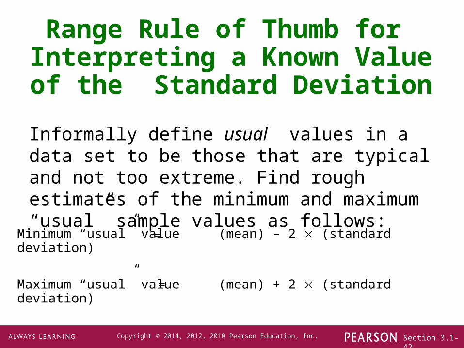
Range Rule of Thumb for Interpreting a Known Value of the

Standard Deviation

Informally define usual values in a data set to be those that are typical and not too extreme. Find rough estimates of the minimum and maximum “usual” sample values as follows:

Minimum “usual” value (mean) – 2 (standard deviation) =

Maximum “usual” value (mean) + 2 (standard deviation) =


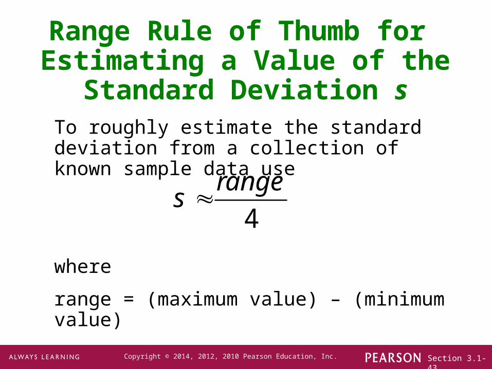
Range Rule of Thumb for Estimating a Value of the

Standard Deviation sTo roughly estimate the standard deviation from a collection of known sample data use

where

range = (maximum value) – (minimum value)

4

ranges


Example

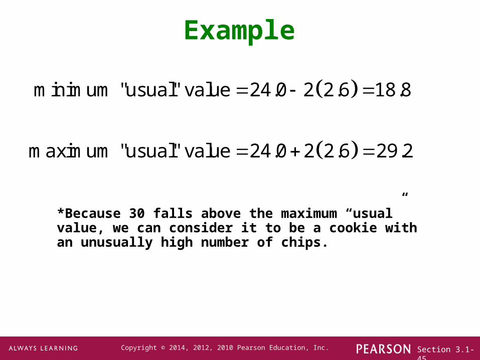
Using the 40 chocolate chip counts for the Chips Ahoy cookies, the mean is 24.0 chips and the standard deviation is 2.6 chips.

Use the range rule of thumb to find the minimum and maximum “usual” numbers of chips.

Would a cookie with 30 chocolate chips be “unusual”?


Example

. . .

. . .

minimum "usual" value 24 0 2 2 6 18 8

maximum "usual" value 24 0 2 2 6 29 2

*Because 30 falls above the maximum “usual” value, we can consider it to be a cookie with an unusually high number of chips.


Comparing Variation inDifferent Samples

It’s a good practice to compare two sample standard deviations only when the sample means are approximately the same.

When comparing variation in samples with very different means, it is better to use the coefficient of variation, which is defined later in this section.


Population Standard Deviation

This formula is similar to the previous formula, but the population mean and population size are used.

2( )x

N


Variance

Population variance: σ2 - Square of the population standard deviation σ

The variance of a set of values is a measure of variation equal to the square of the standard deviation.

Sample variance: s2 - Square of the sample standard deviation s

jarvis01

would make color of sigma to be red just like s especially when the blue font is changed to black


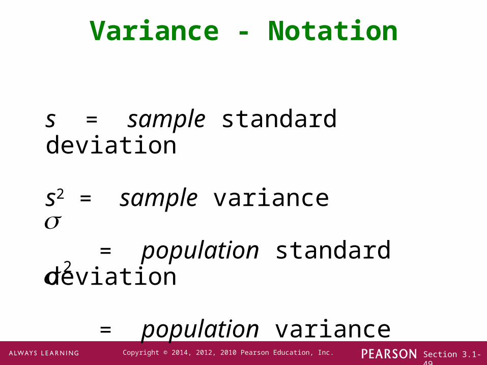
Variance - Notation

s = sample standard deviation

s2 = sample variance

= population standard deviation

= population variance2


Unbiased Estimator

The sample variance s2 is an unbiased estimator of the population variance , which means values of s2 tend to target the value of instead of systematically tending to overestimate or underestimate .

2 22


Beyond the Basics of Variation

Part 2


Rationale for using (n – 1) versus n

There are only (n – 1) independent values. With a given mean, only (n – 1) values can be freely assigned any number before the last value is determined.

Dividing by (n – 1) yields better results than dividing by n. It causes s2 to target whereas division by n causes s2 to underestimate .

22


Empirical (or 68-95-99.7) Rule

For data sets having a distribution that is approximately bell shaped, the following properties apply:

About 68% of all values fall within 1 standard deviation of the mean.

About 95% of all values fall within 2 standard deviations of the mean.

About 99.7% of all values fall within 3 standard deviations of the mean.


The Empirical Rule


Chebyshev’s TheoremThe proportion (or fraction) of any set of data lying within K standard deviations of the mean is always at least 1–1/K2, where K is any positive number greater than 1.

For K = 2, at least 3/4 (or 75%) of all values lie within 2 standard deviations of the mean.

For K = 3, at least 8/9 (or 89%) of all values lie within 3 standard deviations of the mean.


ExampleIQ scores have a mean of 100 and a standard deviation of 15. What can we conclude from Chebyshev’s theorem?

•At least 75% of IQ scores are within 2 standard deviations of 100, or between 70 and 130.

•At least 88.9% of IQ scores are within 3 standard deviations of 100, or between 55 and 145.


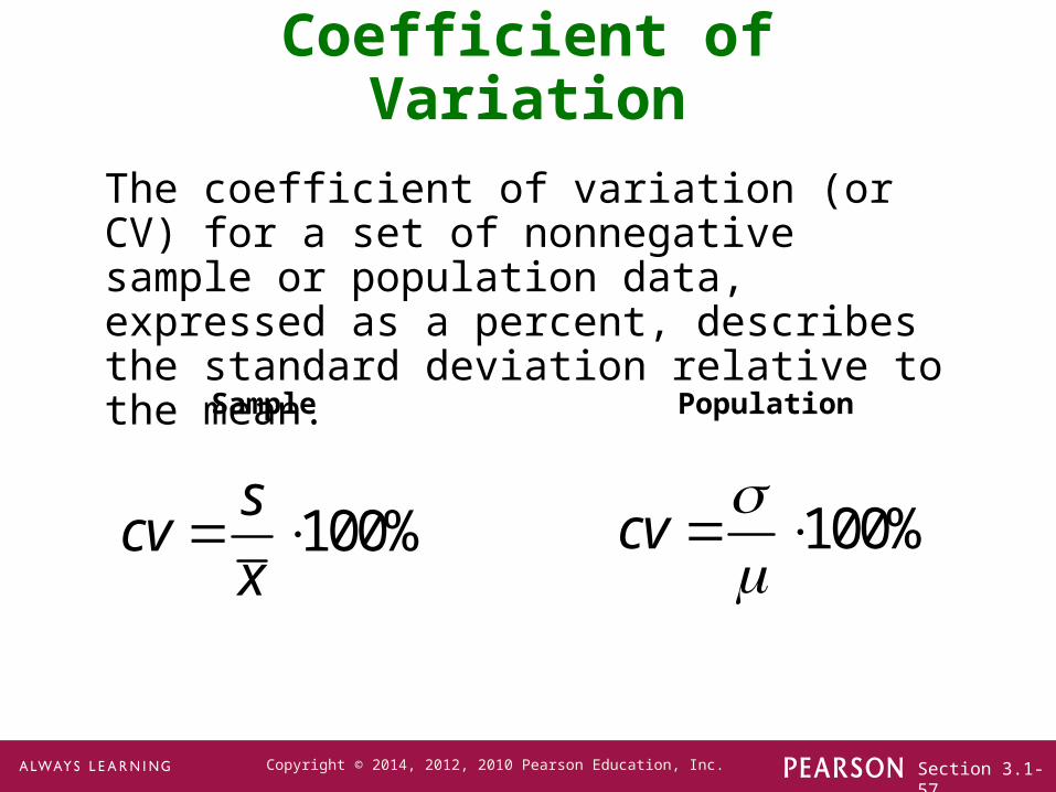
Coefficient of Variation

The coefficient of variation (or CV) for a set of nonnegative sample or population data, expressed as a percent, describes the standard deviation relative to the mean.

Sample Population

100%s

cvx

100%cv


Key Concept

This section introduces measures of relative standing, which are numbers showing the location of data values relative to the other values within a data set.

They can be used to compare values from different data sets, or to compare values within the same data set.

The most important concept is the z score.

We will also discuss percentiles and quartiles, as well as a new statistical graph called the boxplot.


Basics of z Scores, Percentiles, Quartiles, and

Boxplots

Part 1


z Score (or standardized value)

the number of standard deviations that a given value x is above or below the mean

z score

jarvis01

Can you align these two lines so that they align vertically with z? I couldn't move the second line.


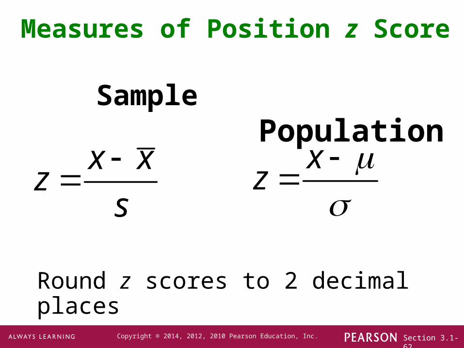
Sample

x xz

s

Population

Round z scores to 2 decimal places

Measures of Position z Score

xz


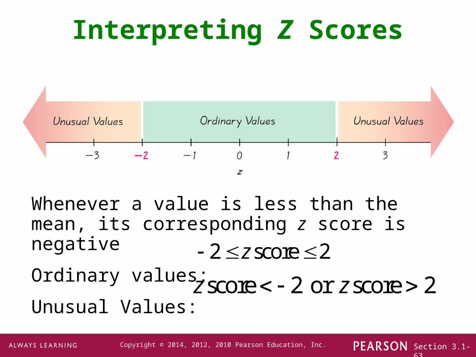
Interpreting Z Scores

Whenever a value is less than the mean, its corresponding z score is negative

Ordinary values:

Unusual Values:

2 score 2z

score 2 or score 2z z


Example

The author of the text measured his pulse rate to be 48 beats per minute.

Is that pulse rate unusual if the mean adult male pulse rate is 67.3 beats per minute with a standard deviation of 10.3?

Answer: Since the z score is between – 2 and +2, his pulse rate is not unusual.

48 67.31.87

10.3

x xz

s


Percentiles

are measures of location. There are 99 percentiles denoted P1, P2, . . ., P99, which divide a set of data into 100 groups with about 1% of the values in each group.


Finding the Percentile of a Data Value

Percentile of value x = • 100number of values less than x

total number of values


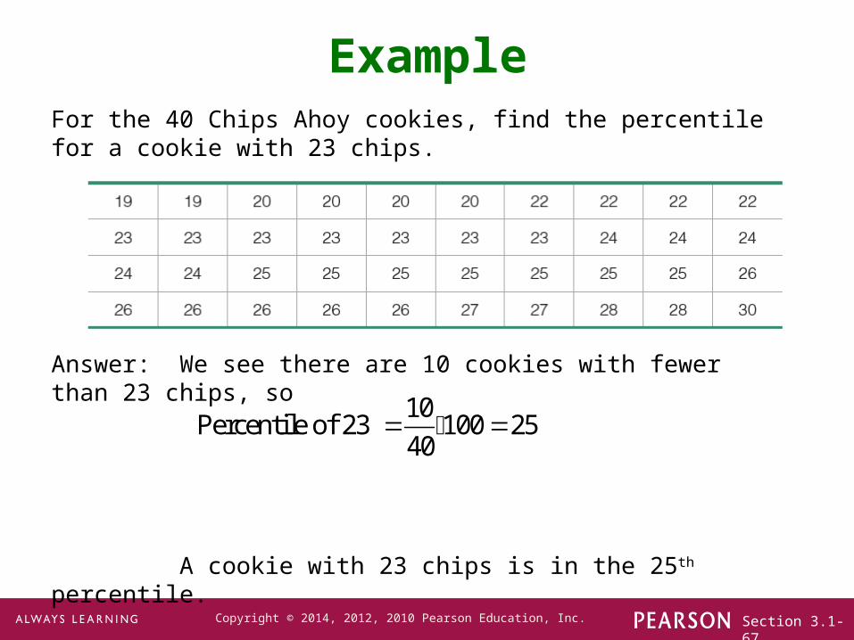
ExampleFor the 40 Chips Ahoy cookies, find the percentile for a cookie with 23 chips.

Answer: We see there are 10 cookies with fewer than 23 chips, so

A cookie with 23 chips is in the 25th percentile.

10Percentile of 23 100 25

40


n total number of values in the data set

k percentile being used

L locator that gives the position of a value

Pk kth percentile

Notation

Converting from the kth Percentile to the Corresponding Data Value

100

kL n


Converting from the kth Percentile to the Corresponding Data Value


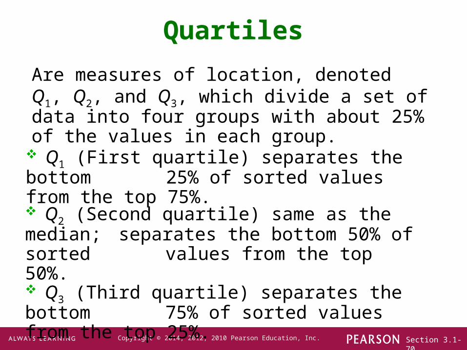
Quartiles

Q1 (First quartile) separates the bottom 25% of sorted values from the top 75%.

Q2 (Second quartile) same as the median; separates the bottom 50% of sorted values from the top 50%.

Q3 (Third quartile) separates the bottom 75% of sorted values from the top 25%.

Are measures of location, denoted Q1, Q2, and Q3, which divide a set of data into four groups with about 25% of the values in each group.


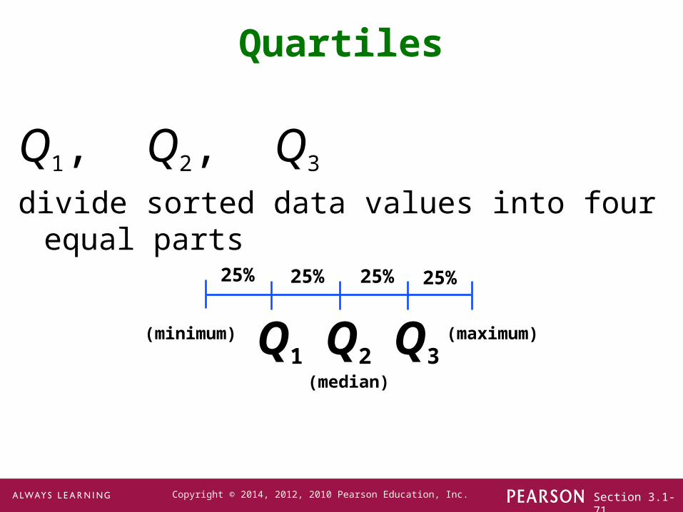
Q1, Q2, Q3 divide sorted data values into four equal parts

Quartiles

25% 25% 25% 25%

Q3Q2Q1(minimum) (maximum)

(median)


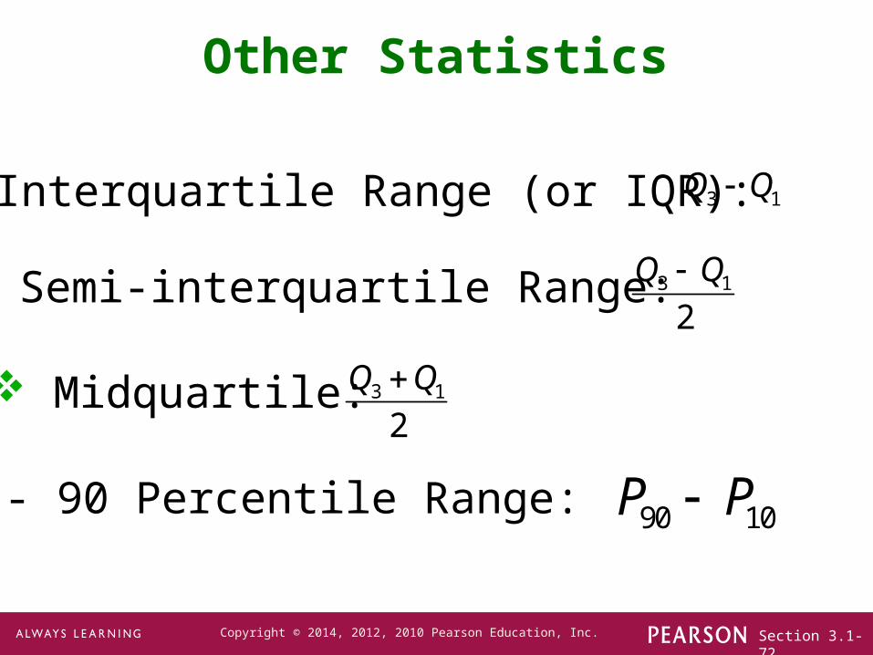
Other Statistics

Interquartile Range (or IQR):

10 - 90 Percentile Range:

Midquartile:

Semi-interquartile Range: 3 1

2

Q Q

3 1Q Q

3 1

2

Q Q

90 10P P


For a set of data, the 5-number summary consists of these five values:

1. Minimum value

2. First quartile Q1

3. Second quartile Q2 (same as median)

4. Third quartile, Q3

5. Maximum value

5-Number Summary


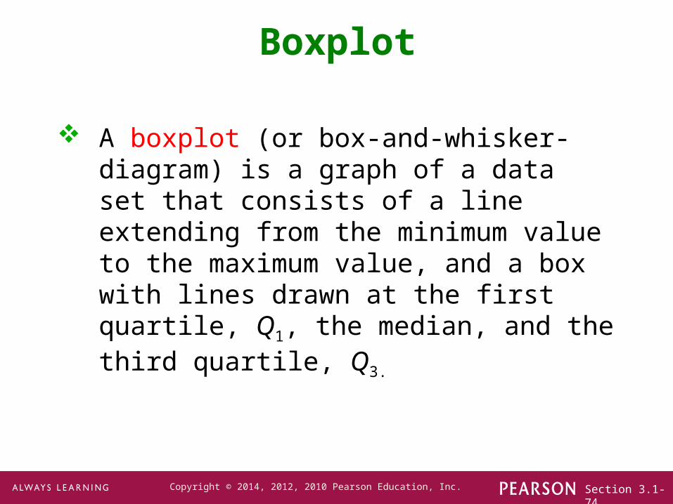
A boxplot (or box-and-whisker-diagram) is a graph of a data set that consists of a line extending from the minimum value to the maximum value, and a box with lines drawn at the first quartile, Q1, the median, and the third quartile, Q3.

Boxplot

jarvis01

Would include a slide on how to construct a boxplot. Would put that slide afterthis one. The procedure is on p. 119.


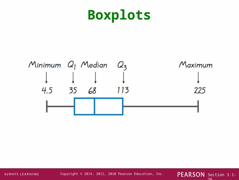
1. Find the 5-number summary.

2. Construct a scale with values that include the minimum and maximum data values.

3. Construct a box (rectangle) extending from Q1 to Q3 and draw a line in the box at the value of Q2 (median).

4. Draw lines extending outward from the box to the minimum and maximum values.

Boxplot - Construction

jarvis01

Would include a slide on how to construct a boxplot. Would put that slide afterthis one. The procedure is on p. 119.


Boxplots


Boxplots - Normal Distribution

Normal Distribution:Heights from a Simple Random Sample of Women


Boxplots - Skewed Distribution

Skewed Distribution:Salaries (in thousands of dollars) of NCAA Football Coaches


Outliers andModified Boxplots

Part 2


Outliers

An outlier is a value that lies very far away from the vast majority of the other values in a data set.


Important Principles

An outlier can have a dramatic effect on the mean and the standard deviation.

An outlier can have a dramatic effect on the scale of the histogram so that the true nature of the distribution is totally obscured.


Outliers for Modified Boxplots

For purposes of constructing modified boxplots, we can consider outliers to be data values meeting specific criteria.

In modified boxplots, a data value is an outlier if it is:

above Q3 by an amount greater than 1.5 IQR

below Q1 by an amount greater than 1.5 IQR

or


Modified Boxplots

Boxplots described earlier are called skeletal (or regular) boxplots.

Some statistical packages provide modified boxplots which represent outliers as special points.


Modified Boxplot Construction

A special symbol (such as an asterisk) is used to identify outliers.

The solid horizontal line extends only as far as the minimum data value that is not an outlier and the maximum data value that is not an outlier.

A modified boxplot is constructed with these specifications:


Modified Boxplots - Example

jarvis01

Would label the boxplot similarly to figure 3-8 on p. 121 so that the lowest and highest data values that are not outliers are identified and the outliers are identified by the dots.


Putting It All Together

So far, we have discussed several basic tools commonly used in statistics –

Context of data

Source of data

Sampling method

Measures of center and variation

Distribution and outliers

Changing patterns over time

Conclusions and practical implications

This is an excellent checklist, but it should not replace thinking about any other relevant factors.

Section 3.1-1 Copyright © 2014, 2012, 2010 Pearson Education, Inc. Lecture Slides Elementary...

Documents

Transcript of Section 3.1-1 Copyright © 2014, 2012, 2010 Pearson Education, Inc. Lecture Slides Elementary...