-1-

SECRETS OF MAGNETO-HYDRODYNAMIC HELL:

The Solar Circulation Paradox and the Geodynamo

Bertrand C. Barrois*

Institute for Defense Analyses

Revised, July 2009

Differential rotation is widely supposed to be essential for the dynamo effects that sustain

solar and planetary magnetic fields, but dynamo effects tend to oppose the flows that

drive them, and it is uncertain what drives differential rotation. The relative sign of the

differential rotation and meridional circulation is not consistent with simple convection

modified by Coriolis forces. We investigate dynamo mechanisms consistent with the

observed solar circulation, and discuss how reactive JxB forces would affect such flows.

We formulate scaling rules that relate the magnetic field strength to mean rotation and

convective heat transport.

Traditional discussions of stellar and planetary dynamos are obscure and

conceptually unsatisfactory. The old language of alpha and omega effects is vague and

begs for better definition. (The alpha effect refers to miscellaneous correlations between

fluctuating magnetic fields and fluid flows, which are presumed to have cross-terms that

regenerate the main magnetic field. The omega effect refers to Coriolis phenomena that

convert poloidal into toroidal flows.)

Kinematic dynamo models, which take a time-independent fluid flow as given,

tell only half the story. It is widely believed that the dynamo effect depends on

differential rotation and/or meridional circulation, which must also be explained. The

signs of these flows are critical to the dynamo, and it seems likely that magnetic as well

as Coriolis forces play a role in driving and/or orienting them.

Some fifty years ago, Bullard & Gellman took the productive approach of

expanding both the magnetic field and the fluid flow in a set of vector spherical

harmonics, and of describing the time-evolution of a kinematic dynamo by coupled

differential equations. But the limitations of their truncated basis soon became apparent,

and ever since, only the foolhardy have dared to simplify.

* Address: IDA, 4850 Mark Center Dr, Alexandria VA 22311. E-mail: BBarrois@ida.org

-2-

Although the lavish simulations now running on supercomputers appear to

contain all the pertinent physics, they are almost too detailed, and it is a challenge to

highlight the relevant patterns and correlations, which is what these notes aim to do.

The Solar Circulation Paradox

Steady flows are observed on the surface of the sun. Rotation is faster at the

equator (25-day period) than at the poles (35-day period). The meridional circulation at

the surface is an order of magnitude slower. It goes from the equator toward the poles,

with a speed approaching 40 m/s at mid-latitudes.

One is immediately tempted to relate these flows via the Coriolis force, but one

must first decide which drives which. Recall that rotations around the z-axis carry X to Y

but carry Y to -X. The relationship depends on who leads, and who follows.

The relative sign of the flows is inconsistent with simple convective mechanisms.

It is easy to see that convection could drive meridional circulation, which brings hot gas

up from the depths. But if the poleward meridional circulation were the driver, the

Coriolis force would make the rotation slower at the equator and faster at the poles,

contrary to fact. If differential rotation were the driver, it should act as a centrifugal

pump, drawing fluid outward at low latitudes, and returning it at higher latitudes, exactly

as observed. But this raises a further riddle: “What could possibly drive differential

rotation?” We will look for explanations in the balance between hydrodynamic forces

and reactive side-effects of the dynamo mechanism.

Fundamental Equations

The time evolution of the magnetic field is governed by the following equation,

which can be derived by assuming that B)v(EJ , and then eliminating E from

Maxwell’s equations. (It is safe to drop the displacement term because slow changes do

not radiate significant amounts of energy.)

)(curlcurl)(curl 1 BBvB

Interpretation: Magnetic field lines are dragged along (“advected”) by the

moving fluid, and are compressed wherever the fluid converges, but tend to diffuse and

dissipate because of finite conductivity. The diffusion term simplifies if the conductivity

() is constant.

B(v)B)v(B)B(vB21div

-3-

The fluid flow is driven by buoyancy, twisted by Coriolis forces, and restrained

by magnetic drag. The buoyancy term is written in terms of excess enthalpy (H) with

expansion coefficient PP CdHVda /]/)(log[ , where H and CP are per gram.

PHa 11 gBJvΩ)v(vv

In our slow-motion approximation, we may assume that the pressure deviation

(P) is chosen to enforce the incompressibility constraint div(v) = 0.

Finally, the excess enthalpy is fed by heat sources and sinks, with ohmic and

hydrodynamic contributions.

HHaJhHH

221)( gvv

Entropy-based accounting would allow us to omit the VdP term, but requires

knowledge of the ambient temperature profile.

HJhTT

SvSo

2211)(

The irreversible diffusion term now generates entropy as well as redistributing it,

thanks to the second-order correlation between T and H. With a little help from

integration by parts, the entropy source is seen to be pCSS / .

The geophysical heat source (h) might be a distributed source such as

radioactivity, while the sink might be heat conduction across the core-mantle boundary.

(A competing hypothesis asserts that the convection is driven by progressive freezing of

the inner core. When pure iron freezes out, streamers of less-dense elements have much

the same buoyancy as heated material. Although the heat of fusion released by freezing

is small, the work done against buoyancy would be vastly greater. In this case, the source

would be localized at the inner boundary, and the sink distributed.)

Settling ultimately converts gravitational potential energy into heat, which is

transported outward to a sink at the outer boundary.

In either case, the equivalent heat transport probably amounts to 1-10 TW. Given

our estimate of the adiabatic temperature gradient at R(outer) = 3580 km, ~ 1.2 deg/km,

heat conduction alone could transport as much as 5 TW, leaving little to be transported by

convection. The settling of denser elements over some five billion years could release

the gravitational equivalent of ~2 TW at R(inner) = 1220 km, and this alternative

mechanism is not prone to serious competition from chemical diffusion, which is much

slower than heat diffusion mediated by conduction electrons.

-4-

In any coarse-grained analysis, thermal and magnetic diffusion are overwhelmed

by turbulent transport, termed hyper-diffusivity, but they are essential in principle to

enable dissipation at short length scales. It is safe to ignore viscosity entirely, because it

does not even enter the MHD stability analysis.

Energy Conservation

Energy takes several forms in the geodynamo -- kinetic, thermal, gravitational,

and electromagnetic -- the sum of which must be conserved second by second.

Moreover, the energy in each of these categories is bounded over the long run. Energy

can slosh back and forth, but there can be no steady transfers between categories.

Magnetic drag draws down the kinetic energy of the fluid at a rate of BvJ ,

while energy is transferred (non-locally) to the electromagnetic fields at a rate of EJ .

Taking the difference, we find that ohmic heating must amount to /2J B)v(EJ .

Since kinetic energy remains bounded, we may conclude that the work done by

buoyancy must ultimately balance the work done by magnetic drag. This consideration

suggests a scaling rule of the form: agFvHagvB ~~22 , where F denotes the

convective heat transport though the system (i.e., flux = power / area). The magnetic

field energy is hundreds or thousands of times greater than the kinetic energy of the fluid.

Such arguments do not reveal where the work is done. Poynting’s vector can

reshuffle electromagnetic energy, and the convection engine can accept heat at one depth

while delivering work at another.

THERMAL

ENERGYKINETIC

ENERGY

B-FIELD

ENERGY

MAG

DRAG

HEAT SOURCE

CONDUCTION THRU

OUTER BOUNDARY

POYNTING

VECTOR

J . E

INERTIAL

CONVECTION

THERMAL

CONVECTION

BUOYANT WORK

OHMIC

HEAT

THERMAL

DIFFUSION

-5-

The dissipation number represents the ratio of work done by buoyancy over the

entire volume (then dissipated by magnetic drag and redeposited) to the net power

transported through the system. It may be estimated as 65.0~agdR .

Magnetic Drag on High-Order Modes

Magnetic drag is not isotropic. A pure BB)v ( force would always oppose

transverse flows, but when the induced currents diverge or dead-end on a boundary,

charge separation will occur, and the resulting E field will offset or cancel Bv . We

may calculate the drag from a uniform magnetic field on a shear flow with )cos(~ xkv

as )))((( vBPBPF

, where the tensor 2/ kkk1P

enforces the constraints

div(v) = div(J) = 0.

Defining 2B , taking 4 gauss for the external dipole field strength

extrapolated into the core, and < 0.6 MS/m for the electrical conductivity, we find 1/ on

the order of a day. (This is suspiciously close to the rotation period. Can it be mere

coincidence? The sun’s ratio of / is three orders of magnitude times greater.)

The toroidal magnetic field internal to the core has no external manifestations but

is thought to be significantly stronger than the external dipole field. The toroidal field

would have no effect on parallel toroidal flows such as differential rotation but could be

the dominant drag on eddies. We will need the language of vector spherical harmonics to

discuss these low-order modes.

Vector Spherical Harmonics

Since both the fluid flow (v) and the magnetic field (B) are divergence-free, it is

convenient to expand them in vector spherical harmonics. These vector functions come

in toroidal and poloidal series, labeled by the familiar quantum numbers L, M, and the

number of radial nodes. They may be constructed as follows, starting with an arbitrary

scalar function F:

)(;)( TSRRT curlFFcurl

Note that the toroidal vector has no radial component, but that if

),()( LMYrfF , the radial component of the poloidal vector will faithfully reproduce

the initial scalar: FLL )1( SR .

The fields and flows obey subtly different boundary conditions. The fluid flow

may not cross a boundary, but its parallel components may slip. The magnetic field must

-6-

join smoothly to a curl-free external field, but its parallel components must taper off

unless there is a surface current. We will use the self-explanatory notation “VS(L,M)”

(and so forth) to describe patterns consistent with these boundary conditions, where U =

steady flow, V = fluctuating flow, B = magnetic field, J = electric current, S = poloidal,

and T = toroidal. Since we are only interested in real functions, we will write (L,M,S)

and (L,M,C) for the sine and cosine functions of azimuth, when the distinction is

significant.

The radial dependence is not indicated. There is no good reason to use spherical

Bessel functions; polynomials are more convenient; and either can be used to construct

an orthonormal basis. It is easy to integrate polynomial functions over the unit ball (the

interior of the unit sphere) using the rule:

!)!3222(

!)!12(!)!12(!)!12(3222

cba

cbazyx

ball

cba

Spherical harmonics are convenient because of the spherical boundary conditions,

but it should be noted that Coriolis forces break the symmetry and that L is a “bad”

quantum number in this problem. Only M and parity are “good” quantum numbers.

There cannot be any correlations between the amplitudes of field and flow components

with different quantum numbers.

It is amusing to note that patterns of the most prominent parities (with respect to

x,y,z or just z) form closed sub-algebras. For example, it would be theoretically possible

to find solutions purely of VS(even,M) + VT(odd,M) + BS(odd,M) + BT(even,M). But

nature seems to have other ideas. The slightest imperfections can mix these patterns with

others of opposite parity, and there is no hint of an even-odd parity imbalance in the

observable geomagnetic field.

The main magnetic field patterns (with a nominal taper) are as follows:

BS(1,0) = )]222(,,[ 222 zyxyzxz from )2/1( 2rzF

BT(2,0) = )1](0,,[ 2rxzyz from )1)(2( 2222 rzyxF

The most prominent flows are meridional circulation and differential rotation:

US(2,0) = )]442(),(),31([ 222222 zyxzsameyzyxx

UT(odd,0) = ]0,,[ xy (untapered)

The conservation of angular momentum demands that all three VT(1,M) flows

remain constant. In a co-rotating frame, they are simply zero.

-7-

Magnetic Drag on Low-Order Modes

We are now in a position to calculate the magnetic drag on low-order modes. The

drag coefficient may be defined as 22

2)(

Bv

EBv . The effects of the pure BT(2,0) field

on VS(L,M) and VT(L,M) flows derived from LM

LYrrF )1( 2 are shown in the table.

It is apparent that magnetic drag is strongest at mid-latitudes, on modes with M ~ L/2.

Magnetic Drag Coefficients due to BT(2,0)

VS(L,M) M=0 M=1 M=2 M=3 M=4

L=1 0.123 0.106

L=2 0.051 0.432 0.202

L=3 0.065 0.247 0.547 0.229

L=4 0.072 0.177 0.415 0.557 0.222

VT(L,M) M=0 M=1 M=2 M=3 M=4

L=1 0 0.434

L=2 0 0.271 0.510

L=3 0 0.176 0.521 0.478

L=4 0 0.117 0.394 0.615 0.418

The calculation says that the toroidal field exerts very little drag on steady

meridional circulation. Moreover, VS(L,0) flows will ultimately distort the toroidal field

so as to further reduce the drag. In the absence of diffusion and/or turbulent transport,

the steady state would have 0)( Bvcurl , and E would cancel Bv . This

leaves the external (poloidal) field extrapolated into the core as the dominant drag on

steady flows.

Convective Stability Analysis

The Bénard analysis of convective instabilities can be heuristically adapted to

reveal the modes that are active after the onset of convection. An eigenvector analysis of

temperature variations, poloidal, and toroidal flows, coupled by buoyancy and Coriolis

forces, suggests that there are three families of modes. In the case of eddies with M>0,

there is a marginally unstable convection mode (restrained only by turbulent transport

phenomena) as well as two strongly damped flow modes. The marginally stable mode is

a “magnetostrophic flow” or “thermal wind”, of the sort used by Graeme Sarson to drive

kinematic dynamos.

-8-

Let denote the deviation from ambient temperature, the mean super-adiabatic

temperature (or composition) gradient, and the thermal expansion (or buoyancy)

coefficient. The linearized equations of motion are

0)(;; vvβΩvgvvθ divP

If we were to neglect the anisotropic effects, namely magnetic drag and Coriolis

forces, the unstable modes (with growth rate ) would emerge as pure L-states from a

generalized eigenvalue problem:

Fr

LLF

2

22 )1()(

gθ with ))(( FcurlcurlvS R

Both magnetic drag and advection by differential rotation tend to mix (L,M)

modes with (L±2,M), provided that M≠0.

If we single-out a specific VS(L,M) mode and neglect its couplings to other

poloidal modes of like parity, the truncated eigenvalue problem takes the form shown

below, with inhomogeneous driving terms added. Let S denote the VS(L,M) velocity,

and T the VT(L±1,M) velocity. Furthermore, let S,T denote the rate(s) of damping due to

magnetic drag, the effective Coriolis parameter related to the rotation rate, g the

effective buoyancy coefficient, and the damping due to turbulent heat transport. All

parameters are defined to be positive, while S & T are positive in the observed directions

(i.e., poleward at the surface, prograde at the equator.)

T

S

T

S

F

F

F

T

Sg

T

Sdt

d

0

0

The effective buoyancy coefficient and Coriolis parameter depend on (L,M) via

2

))(()(

S

effv

αg

vgθv ;

22

2

2

TS

TS

effvv

vΩv .

In a thin shell, representative of the sun’s convective zone, the value of (g) is

greater for L=2 than for L=1. This seems to hold true in the earth as well, although the

temperature and/or composition gradients are poorly known.

The boundedness of the system forbids positive eigenvalues, because they would

indicate runaway growth. Hence, turbulence must build to the point where turbulent

transport phenomena that mimic diffusion can restrain the most unstable mode,

presumably VS(2,0).

-9-

2

TS

Tg

(A similar analysis applies to high-order modes characterized by wave-vector k.

Careful calculation shows that at every latitude , there exists one direction of k at which

magnetic drag is ineffectual and the undamped growth rate approaches g)sin( , but

this exceptional case does not seem to set any time scales.)

The concept of eddy viscosity is somewhat bogus, because genuine diffusion

coefficients have units of L2/T, whereas Kolmogorov’s theory of turbulence maintains

that power spectra and correlation times can be derived by dimensional analysis from a

parameter with units of L2/T

3, which represents the power per unit mass cascading from

low-order to high-order eddy modes. It follows from dimensional analysis that eddy

decay rates scale as the 2/3 power, not the square, of spatial frequency.

If we swallow our misgivings about the effective diffusion coefficient , we can

derive an approximate relationship between and v. Taking 2)/(~ R and

PCF /~ midway between the inner and outer boundaries, we find )/(~ Rv .

The damping time constant 1/ must be on the order of centuries, whereas 1/ is on the

order of hours to days, depending on the strength of the toroidal magnetic field.

These arguments allow us to estimate the Nusselt number, which represents the

renormalization of thermal conductivity by turbulent transport. According to accepted

heuristics, the local temperature gradient should diverge as(x) ~ 1/x when approaching

a boundary, but the divergence cuts off where conduction takes over from convection.

The average temperature gradient T/R will exceed the central gradient dT/dR by a

logarithmic factor of order ~ log(/o). (Beware unknown factors of order unity.)

The inverse matrix reveals the flows in response to various kinds of zero-

frequency driving terms. (Note that det < 0, and that a positive entry signifies positive

response. The relationship of poloidal to toroidal responses is considered “normal” if

0/~/ TTS , which holds for thermally and/or poloidally driven eddies.) By this

definition, the paradoxical solar circulation is considered “abnormal”.

T

S

S

TT

TTS

F

F

F

gg

g

T

S

)(

)(

det

1

2

The sign of a toroidal response to a toroidal driver (the lower-right entry) is

ambiguous. If barely satisfies the stability bound, the net coefficient could be negative,

-10-

and a prograde force could produce a “perversely” retrograde response, or vice versa.

(Think of a sailboat tacking against the wind.)

“Perversity” notwithstanding, the ratio of meridional circulation to differential

rotation would be strictly “normal” in the limit of marginal stability, contrary to nature.

(We gather that the system must operate close, but not too close, to the stability bound.)

The “perverse” response diverges as approaches the stability bound and the

determinant approaches zero. What limits it? We might argue that runaway differential

rotation over-amplifies the BT(2,0) field, thereby self-quenching. (Once again, the

system must operate close, but not too close, to the stability bound.)

We may try to reproduce the observed relationship with a combination of drivers.

It should be self-evident that thermal drivers based on PCJ /2 can be neglected given

high conductivity. The relative importance of different drivers involves the dissipation

ratio, the magnetic diffusion time scale, and the magnetic drag parameter:

1~~2

2

SSPS R

agR

C

g

JB

JS

F

F

We now have a 2x2 matrix. The observed combination of slow meridional

circulation and fast differential rotation demands that TTS FF /~/ , and there is

nothing “perverse” about the sign of the required toroidal driver.

T

Sg

F

F

T

S

T

S

)/(

Effects of Steady Flows

It is often said that conducting fluids drag field lines, but this statement is naive.

If the core rotated as a rigid body, it would have no such effect on a uniform field parallel

to the axis of rotation, because charge separation would establish an E field that cancelled

V×B. This follows from the fact that (×R)×B is curl-free and can be canceled by

This would also be true of rotation-on-cylinders, but the effect of latitude-

dependent differential rotation or rotation-on-planes is to shear the field lines into

hairpins, thereby creating a strong toroidal field, predominantly BT(2,0).

It is possible to set up an idealized problem by abandoning spherical geometry in

favor of straight lines of flow. The effect of a z-directed flow on an x,y-directed field,

-11-

both z-independent, is to create an additional z-directed field that may be calculated from

zz vB )(2 B .

The effect of meridional circulation is to distort the field lines with a touch of

BS(3,0) and ultimately to roll them up. It is possible to solve an idealized “jelly roll”

problem exactly, again by abandoning spherical geometry, with Hankel functions of

complex argument, but the solution is physically unrealistic because the field strength is

amplified by a factor of exp(2) = 535.5 per turn of the spiral, thereby imposing

prohibitive magnetic drag. (This factor is suspiciously close to the number of voting

members of the U.S. Congress. Can it be mere coincidence?) One valuable lesson from

the jelly roll model is that the circulation time cannot be much shorter than the diffusion

time. The exact time-independent solution takes the form:

)]exp()/(Re[...

)(curl :Internal

)sin(;1 :External

)0,,(:nCirculatio

1

2

iirHA

AiA;

ryAB

xy

z

zzz

zx

AB

v

(The coefficient must be chosen to join smoothly to the external field. A central

singularity is inevitable but inoffensive because the total field energy is log-divergent.)

Effects of Eddies

It is possible to make up hypothetical VS(L,M) eddies accompanied by Coriolis-

twisted VT(L±1,M) eddies and to calculate their combined effects on the magnetic field.

These eddies may be somewhat unrealistic in terms of latitude and radial profiles,

because L is a “bad” quantum number. (Strictly speaking, we should be considering

uncorrelated normal modes, as defined by the Karhunen-Loeve decomposition, involving

diagonalization of a covariance matrix of temperatures and/or velocities at many points.

It is difficult to identify these normal modes a priori, except in translationally invariant

systems.)

A key step in constructing the Coriolis-twisted sidekick is to extract the

solenoidal part of Ωv . This involves subtracting the gradient of a scalar, chosen to

cancel any divergence and/or flow through the boundary. Computationally, the best

method is to construct a complete, orthonormal basis of solenoidal functions of sufficient

degree. Unless the original pattern is a mixture of many different harmonics, the

functions can be generated by repeated application of the operator ))(1)(( 2 curlrcurl ,

followed by Gram-Schmidt orthogonalization. Double-precision arithmetic is essential.

-12-

The geometric effect of a VS(L,M,C) eddy is to distort BS(1,0) to a linear

combination of BT(L,M,S) and BS(L±1,M,C). The same eddy can then act a second time

to regenerate BS(1,0). The same is true for the accompanying VT(L±1,M,C) eddy, which

distorts BS(1,0) to a combination of BT(L,M,C) et cetera. However, it turns out that the

sign of the regeneration coefficient is negative. Instead of amplifying the field, two-stage

mechanisms act to diffuse it.

Only VS×BT and VT×BS terms contribute to the dipole moment. Since VT×BT

is purely radial, it cannot generate a JT(1,0) current loop. VS×BS is also impotent, for a

subtler reason. If / were uniform, the contribution of VS×BS to the dipole moment

would integrate to zero. (Quick proof: Consider the M=0 case, in which all flow and

field lines form closed loops in a plane. If a flow line crosses a field line outbound, it

must cross the same field line inbound elsewhere. The result can be extended to M>0

using Wigner’s theorem. Since the Clebsch-Gordan coefficients for (L,M; L±1,-M; 1,0)

do not vanish when M=0, we may conclude that the universal coefficient does.)

Even if / were significantly non-uniform, all reasonable VS×BS mechanisms

(in which the conductivity is a function of depth and/or temperature) seem to produce

damped oscillations. The picture below shows the poloidal flow carrying nested field

lines around in a grand tour. There is no current density at the center of the nested field

loops to counter ordinary ohmic decay. Moreover, the prograde current cannot cancel

the retrograde current due to subtle variations of conductivity because they are at the

same depth.

-13-

Flow transports

magnetic loops

FLOW

FIELD

” VxB > 0

’ VxB < 0Conductivity (P)

varies with depth

(later)

(now)

Pictorial Proof of Cowling’s Theorem

These results are consistent with Cowling’s Theorem, which maintains with great

generality that axisymmetric flows cannot sustain axisymmetric fields, even in the time-

dependent case. The CG coefficient for (L,M; L,-M; 1,0) is proportional to M and

vanishes for M=0. Second-order coefficients will be seen to scale precisely as M2.

We may define dipole “degeneration” coefficients for B = BS(1,0) as follows:

2/122

))((]0,,[

Bv

curlxy Bvv

Dipole Dissipation Coefficients, Two-Stage

VS(L,M) M=0 M=1 M=2 M=3 M=4

L=1 0 -2.08

L=2 0 -0.75 -3.01

L=3 0 -0.39 -1.59 -3.57

L=4 0 -0.25 -1.54 -2.23 -3.96

-14-

Three-Stage Dynamo Mechanisms

Although two-stage mechanisms seem utterly hopeless, some three-stage

mechanisms can produce positive regeneration. For example, an “alpha-omega” effect:

Steady differential rotation pre-distorts BS(1,0) to BT(2,0).

A VS(L,M) eddy distorts BT(2,0) to BS(L±1,M)

Its VT(L±1,M) sidekicks distort BS(L±1,M) to regenerate BS(1,0).

Intermediate BT(L,M) patterns would be allowed by parity, but direct

calculation shows that they are not generated. Moreover, VS×BT terms

cannot contribute to the dipole moment.

The eddies can act in either order with identical effect. The catch is that some

high-M eddies produce strongly negative regeneration, and we would need to explain

them away. As we have seen, magnetic damping is actually stronger on medium-M

eddies at mid-latitudes, but the ratio of nonlinear drivers is unknown.

The figure illustrates the current component that generates the dipole moment,

averaged with respect to longitude. (Prograde is regenerative; retrograde degenerative.)

The predominantly prograde current loops are characteristically split between the

hemispheres, but the sign of the octupole (L=3) moment is not immediately obvious.

PROGRADE

RETROGRADE

Azimuth-Averaged Toroidal Currents for L=3, M=2, in Vertical Plane, and Actual Azimuthal Distribution in a Mid-latitude Horizontal Plane

We may define dipole regeneration coefficients for BS(1,0) as follows, where

u = UT(3,0), v = VS(L,M), and v’ = solenoidal (v×):

-15-

2/12

2/122

)))(((]0,,[

Buv

curlcurlxy Buvv

Dipole Regeneration Coefficients, Three-Stage, UT-VS-VT

UT-VS-VT M=0 M=1 M=2 M=3 M=4 M=5 M=6 M=7 M=8

L=1 0 -0.223

L=2 0 0.128 -0.726

L=3 0 0.120 0.152 -1.187

L=4 0 0.098 0.263 0.089 -1.152

L=5 0

L=6 0 0.070 0.227 0.386 0.381 -0.074 -1.849

L=7 0

L=8 0 0.042 0.168 0.333 0.483 0.542 0.391 -0.171 -1.868

A competing “alpha” effect (with opposite sign) that does not depend upon

differential rotation could be responsible if high-M eddies are dominant:

Steady meridional circulation pre-distorts BS(1,0) to BS(3,0).

A VS(L,M) eddy distorts BS(3,0) to BT(L,M).

The same eddy distorts BT(L,M) to BS(1,0).

Dipole Regeneration Coefficients, Three-Stage, US-VS-VS

US-VS-VS M=0 M=1 M=2 M=3 M=4 M=5 M=6 M=7 M=8

L=1 0 1.521

L=2 0 -0.306 2.451

L=3 0 -0.244 -0.200 2.467

L=4 0 -0.184 -0.486 -0.158 2.047

L=5 0 1.448

L=6 0 -0.116 -0.418 -0.764 -0.915 -0.539 0.790

L=7 0 0.133

L=8 0 -0.080 -0.314 -0.648 -1.023 -1.337 -1.464 -1.232 -0.502

The high-M current loops are concentrated at low latitudes, and the sign of the

octupole (L=3) moment seems consistent with the observed multipole expansion of the

geomagnetic field, despite the retrograde loop near the boundary.

-16-

Azimuth-average Toroidal Currents for L=2, M=2, in Vertical Plane, and Actual Distribution in Equatorial Plane. Alpha mechanism.

By themselves, the coefficients give an incomplete picture of relative strength,

because the ratio of UT×VS×VT to US×VS×VS effects is enhanced by the ratio of steady

UT(2,0) to US(1,0) flows, which is a mystery, but also suppressed by the ratio of

VT(L±1,M) to VS(L,M) eddies, roughly T/ . (Further arguments will suggest that the

mystery ratio is just big enough to make the two dynamo mechanisms competitive.)

For reasons that will soon become perfectly clear, the steady flow must act either

before or after the rapidly fluctuating flows, to avoid suppression of high-frequency

effects. But steady differential rotation cannot act last, because UT(odd,0)×BS(even,0)

has no azimuthal component to regenerate JT(1,0).

Time Dependence

The effect of a fluctuating eddy is to produce a fluctuating magnetic field. We

may single out a Fourier component: )cos(~)( tvtv o . Suppose that the composite eddy

distorts a steady BT(2,0) to BT(L,M) to BS(1,0). Let A,B,C denote the amplitudes of

these field modes. Taking the ordinary decay rates of these modes into account, we have

coupled evolution equations:

CBtvCBAtvB )(;)(

-17-

Then taking A(t) = 1, we find 22

)cos()sin()(

ttvtB o . The in-phase term

combines with v(t) to regenerate a steady field: 22

2

ov

C . Since the

fluctuating flow is not truly periodic, we should average over its bandwidth , roughly

the reciprocal of its correlation time.

1/

222222d

It seems ironic that the decay rate plays a key role in regeneration but ultimately

drops out of the numerator. Without it, B(t) and V(t) would be strictly out of phase.

In summing over active eddy modes, we should get something commensurate

with the decay rate due to pseudo-diffusion: /~)( 2vo . However, this will be

suppressed by a factor of T/ if it depends on cross-terms between VS and VT.

A Marvelous Toy

It is amusing and instructive to consider what would happen in a two-stage model

if the regeneration coefficient were positive. Conflating A with C, we get

CBtvCBCtvB )(;)(

Were it not for the decay terms, v(t) would simply drive any (B,C) state along a

hyperbola of constant (say positive) // 22 CB . Assume that the state were driven far

out along the asymptote. Given , the decay terms could then pull the state to a new

hyperbola, so that the B-intercept would grow. Paradoxically, one drives this system by

damping it, and it naturally settles into the Methuselah mode.

Unfortunately, this is a poor representation of the three-stage process, because the

stage that converts BS(1,0) into BT(2,0) is slow, and the latter is virtually constant.

Reactive Force Terms

The steady meridional circulation and differential rotation will be affected by the

dynamo’s own J×B reactive force terms.

Suppose that a VS(L,M) eddy distorts BT(2,0) to B’, whereas its toroidal

sidekick VT(L±1,M) distorts BT(2,0) to B”. The FS driver for meridional circulation

comes primarily from B"J"B'J' whereas the FT driver for differential rotation

comes from B'J"B"J' .

-18-

The driver coefficients have been normalized to equal values of 2

Sv and 2u ,

where u may be either US(2,0) or UT(3,0). Their signs are completely consistent.

Drivers for Steady UT(3,0) and US(2,0) Circulation

Diff. Rot. M=0 M=1 M=2 M=3 M=4

L=1 0 -6.0

L=2 0 -16.1 -13.9

L=3 0 -14.4 -45.9 -17.5

L=4 0 -6.7 -63.5 -66.5 -18.0

Mer. Circ. M=0 M=1 M=2 M=3 M=4

L=1 4.7 7.2

L=2 25.3 9.9 1.2

L=3 23.2 24.2 10.5 1.4

L=4 19.2 27.2 21.4 10.5 6.3

Direct calculation confirms that the toroidal force terms oppose the observed

differential rotation, which is obviously not what we want. And the poloidal force terms

drive meridional circulation in the observed direction, which is paradoxically not what

we want, because we need something to slow it down.

Referring back to the 2x2 matrix relationship between drivers and responses, we

find that the observed combination of slow meridional circulation and fast differential

rotation demands that TTS FF /~/ . (And we now pull out what is left of our hair.)

The conservation of energy illuminates the paradox. One of our candidate

dynamo mechanisms involves a conspiracy of differential rotation, poloidal, and toroidal

eddies. Conservation of energy requires that the dynamo mechanism oppose one or more

of the motions that drive it, but perhaps not all three. Indeed, direct calculation of the

toroidal drivers confirms that they oppose the observed differential rotation.

As for magnitudes, the matrix relationship between drivers and responses

demanded that extTTS FF //~/ , which could potentially be reconciled with

/~)/(~"/'~/ inteddyTS TSBBFF . But that is small consolation when the signs are

wrong.

The second dynamo mechanism involves a conspiracy of meridional circulation

and poloidal eddies, but BT(2,0) plays no role. These flows distort BS(1,0) to BS(3,0)

and thence to B, and indeed we find that the reactive J×B force opposes the meridional

-19-

circulation. However, the B’ field derived from distorting BT(2,0) is even stronger, so

B'J' overwhelms J×B and drives meridional circulation in the observed direction,

which is not what we want.

What drives differential rotation?

If not the dynamo’s own reactive forces, then what? We must look to

hydrodynamic terms: STTS vvvv )()( . These advection terms would sum to zero

by symmetry if all M-states of given L had equal kinetic energy, but that seems unlikely.

The high-M eddy modes help to drive differential rotation in the observed direction,

whereas low-M modes (M<<L) have the opposite effect.

Eddy velocities should be fastest in the equatorial plane because the main BT(2,0)

field goes through zero there.

Summary: Are we well done yet?

Do we know enough to predict the magnitude of the externally observable dipole

field? Energy balance tells us that agFvBv ~22

int

2

int , but how are we to separate the

eddy velocity from the internal field strength, and then relate the latter to the external

field strength?

Naive dimensional analysis is ultimately inconclusive because we have a choice

among three very different time scales: rotational , thermodynamic 3 2/ RagF ,

and magnetic diffusion 2/1 R . The simplest possible scaling rule would be ......... )()()( , with exponents that sum to one, but dimensional analysis admits

arbitrary functions of dimensionless ratios: )/,/( f .

We would need a system of interlocking relationships among these three known

parameters and four unknown parameters: internal field strength, external field strength,

differential rotation, and eddy velocity. But unfortunately, our current understanding of

differential rotation and the regeneration mechanism are too sketchy.

The Bootstrap Paradox

In the beginning, God created the heavens and the earth. But what about Hell?

The usual answer is that the dynamo mechanism must have amplified a weak magnetic

seed field, but this is easier said than proven.

-20-

The analysis of convective instability says that Coriolis forces are a stabilizing

influence, and that the growth rate → 0 as the magnetic drag → 0.

Moreover, Taylor’s Theorem says that, absent dissipative or advection forces,

Coriolis forces should regiment the flow into z-independent columns unfavorable to

dynamo action. (Quick proof: Take the curl of P10 Ωv .) It takes either

turbulence or magnetic drag to buck the tyranny of Taylor columns. If the dynamo was

inefficient at start-up, we must explain how it managed to overcome ohmic diffusion.

The scaling rules formulated above suggest that Coriolis dominance does not

suppress the magnetic field, and this may point the way to a resolution of the paradox.

Dominance of Low-Order Eddy Modes

In every discussion of turbulent eddies, it is obligatory to quote Jonathan Swift:

Great fleas have little fleas upon their backs to bite ‘em,

And little fleas have lesser fleas, and so ad infinitum.

And the great fleas themselves, in turn, have greater fleas to go on;

While these again have greater still, and greater still, and so on.

We have mentioned that pseudo-diffusion coefficient is a sum over eddy modes,

without inquiring about the contribution of individual modes.

The existence of multiple time scales could undermine the elementary argument

from dimensional analysis commonly used to justify the Kolmogorov spectrum, but the

spectrum nevertheless seems correct because only one family of convective modes is

unstable, while the others are strongly restrained. The Kolmogorov spectrum derives

from a parameter with units of L2/T

3, here v

2, and the spatial frequency k. We want the

combination that has units of L2/T:

3/43/1

223

3

~/ kvVk

kd

The integral over spatial frequency has a low-k cutoff imposed by the dimensions

of the system and converges slowly at high k.

Unfortunately, this argument gives no clue about the distribution with respect to

angular quantum numbers. The activity in any mode can be estimated from the quotient

of a nonlinear driving term, divided by the net decay rate or effective bandwidth of that

mode. For high-order modes, the decay rate () due to pseudo-dissipation scales as k1,

and overwhelms the growth rate (g/). The fact that magnetic drag is very low for

axisymmetric (M=0) flows and highest at mid-latitudes (M~L/2) becomes irrelevant.

-21-

We dare not conclude that isotropy is restored for high-order modes, however, because v

still has preferred directions on account of buoyancy and couples to k via )(v .

Field Reversals

No discussion of dynamo mechanisms is complete without a bit of irresponsible

speculation on the subject of field reversals.

We have seen that eddy modes participate in the candidate dynamo mechanisms

with inconsistent signs. If there exist eddy modes that contribute positively to pseudo-

diffusion but negatively to regeneration, they may be characterized as “anti-dynamo”

modes that might be responsible for flipping the dipole field.

Hypothesis: An n-sigma fluctuation of anti-dynamo modes can provoke a field

reversal. The frequency of occurrence is )2/exp( 2n per correlation interval ~ 1/.

Since an anti-dynamo mode must act via a two-stage process to cause a reversal,

the effect of a fluctuation is proportional to n2v

2. It follows that an n/2-sigma fluctuation

sustained for 4 would be equally potent, but it would occur just as rarely. Several anti-

dynamo modes might cooperate to provoke a reversal, but the basic result is the same,

and v2 should be understood as a sum over all anti-dynamo modes.

How are we to explain why the sun’s dipole field has been oscillating in recent

centuries on a fairly regular 22-year cycle, whereas the earth’s field reverses at erratic

intervals? (There were no reversals during the cretaceous superchron, which lasted

almost 40 million years. The average interval between reversals then slid gradually to

200,000 years, but there have been no reversals during the last 780,000 years, known as

the Brunhes epoch. As for the sun, there were no spots during the Maunder minimum,

1645-1715 AD.)

One hypothesis is that the sun’s field configuration “rotates” between two states

under the influence of a persistent anti-dynamo flow mode. The trouble is that all known

flow modes produce externally observable BS(L,M) fields, along with confined BT(L,M)

fields, but other BS(L,M) modes are not especially prominent during reversals. For

example, VS(1,1) could interconvert BS(1,0) and BT(1,1), but it would also produce

measurable BS(2,1). It has been reported that the BS(1,0) field is appreciably

contaminated with BS(2,2), which indicates the influence of VS(3,2) and VT(2,2).

-22-

A more elaborate hypothesis is that some coherent combination of BS(L±even,M)

and BT(L±odd,M) could “rotate” the main field to a purely toroidal combination of

BT(L±even,M) patterns and back. The toroidal fields would be strictly internal.

Although axisymmetric (M=0) flows are sometimes capable of inducing damped

oscillations of the dipole moment, their influence in the sun can be ruled out on several

grounds. First, is essentially constant, except for a logarithmic factor, and second,

the meridional circulation time is an order of magnitude shorter than the 22-year

oscillation period. (Consolation: There is evidence of a weak 2-year cycle.)

Summary: What needs to be done?

The mechanisms that we have proposed are not robust. There is a tug-of-war

between opposing US-VS-VS and UT-VS-VT effects, which seem to be of comparable

strength, the winner to be decided by the relative amplitude of various eddy modes, and

the balance between regeneration and turbulent diffusion is equally delicate.

The picture painted here raises a multitude of hard issues of nonlinear dynamics

that I will leave for you to ponder:

Symmetry arguments alone cannot identify the normal modes of the system.

Can they be identified by approximations short of detailed simulation?

Can the power spectrum and time scales of the dominant low-order flow

modes be estimated by studying a severely truncated nonlinear system?

How close to the stability bound does the dynamo operate?

Dimensional analysis is a blunt instrument. Can the saturation values of the

internal and external Elsasser ratios be pinned down?

How do the mean values of steady fields compare to the RMS values of

fluctuating fields? Is it legitimate to calculate magnetic drag on the

assumption that steady BT(2,0) is dominant?

-23-

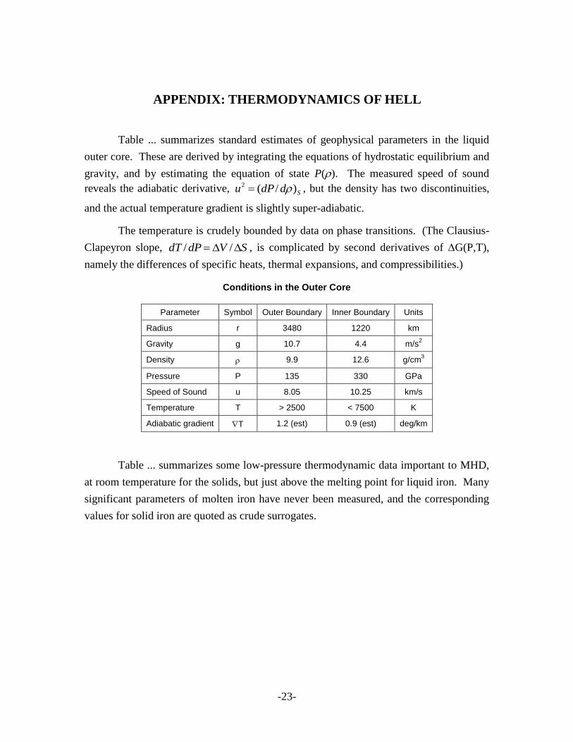
APPENDIX: THERMODYNAMICS OF HELL

Table ... summarizes standard estimates of geophysical parameters in the liquid

outer core. These are derived by integrating the equations of hydrostatic equilibrium and

gravity, and by estimating the equation of state P(). The measured speed of sound

reveals the adiabatic derivative, SddPu )/(2 , but the density has two discontinuities,

and the actual temperature gradient is slightly super-adiabatic.

The temperature is crudely bounded by data on phase transitions. (The Clausius-

Clapeyron slope, SVdPdT // , is complicated by second derivatives of G(P,T),

namely the differences of specific heats, thermal expansions, and compressibilities.)

Conditions in the Outer Core

Parameter Symbol Outer Boundary Inner Boundary Units

Radius r 3480 1220 km

Gravity g 10.7 4.4 m/s2

Density 9.9 12.6 g/cm3

Pressure P 135 330 GPa

Speed of Sound u 8.05 10.25 km/s

Temperature T > 2500 < 7500 K

Adiabatic gradient T 1.2 (est) 0.9 (est) deg/km

Table ... summarizes some low-pressure thermodynamic data important to MHD,

at room temperature for the solids, but just above the melting point for liquid iron. Many

significant parameters of molten iron have never been measured, and the corresponding

values for solid iron are quoted as crude surrogates.

-24-

Low-Pressure Thermodynamic Data

Parameter Symbol Solid Fe Liquid Fe Solid Hg Liquid Hg Units

Temperature -- room 1811 (MP) 234 (MP) room Kelvin

Molar Mass m 55.85 55.85 200.6 200.6 g/mole

Molar Volume V 7.1 8.0 14.13 14.80 cc/mole

Density 7.9 7.0 14.20 13.55 g/cm3

Bulk Modulus -VdP/dV 171 ??? 24.75 27.00 GPa

Speed of Sound u 5.15-5.95 ??? ??? 1.41 km/s

Heat Capacity CP 6.0 9 (solid) 6.60 6.65 cal/deg/mole

Entropy of Fusion S 2.8 2.8 2.33 2.33 cal/deg/mole

Thermal Expansion 35

80 48 180 10-6

deg-1

Thermal Conductivity -- 80 35 (solid) ??? 8.34 W/m/deg

Electrical Conductivity 10.0 0.6 (est.) ??? 1.04 MS/m

Grüneisen Parameter VdP/TdS 1.7 3.0 (est.) 0.6 2.6 --

The heat capacity of an ideal harmonic solid should be about 6 cal/deg/mole.

Solid iron has precisely this value at room temperature, but its heat capacity continues to

rise, peaking near the Curie temperature at 1044 K and approaching 9 cal/deg/mole for

-iron at 1500 K. Much of the excess heat capacity is associated with fluctuations of the

magnetic order parameter.

The speed of sound in solid iron depends on how it is measured. The speed of

sound in a thin fiber depends on Young’s modulus (~210 GPa) but the speed of sound in

bulk matter depends on the C11 modulus (~280 GPa) rather than the bulk modulus for

isotropic compression (~170 GPa). Young’s modulus presumes no transverse stress,

whereas C11 presumes no transverse strain. These moduli can be related by Poisson’s

ratio, p ~ 0.29, defined as the ratio of transverse expansion to longitudinal compression

under unidirectional stress.

)21(3'

pBulk

sYoung

2

11

21

1

' pp

p

sYoung

C

Another key parameter is the thermal expansion coefficient, but it is futile to

extrapolate low-pressure data, because thermal expansion at great depths would entail a

huge amount of work against pressure. However, this coefficient can be related to better

known parameters by the chain rule. (For solids, use the bulk modulus in place of mu2.)

-25-

V

P

VSPP TdS

VdP

mu

C

TdS

VdP

VdP

dV

dT

TdS

VVdT

dV

2

1

The dimensionless ratio VTdSVdP )/( , known as Grüneisen’s parameter, varies

widely, but there is reason to believe that it varies slowly with density. Some of the data

needed to calculate it for molten iron are missing. Using rough surrogates, we can

estimate the mean adiabatic temperature gradient as ~1.1 deg/km, which leaves ample

room for a super-adiabatic gradient to drive the convection. (The derivation uses the

Maxwell relationship that follows from dH = TdS + VdP, as well as the chain rule.)

2u

gT

TdS

VdP

dS

dVg

dP

dTg

dz

dT

VPSS

The physical basis of Grüneisen’s parameter relates to the anharmonicity of the

interatomic potential, and the actual value is consistent with stiff short-range repulsions.

Consider a cubic lattice with spacing 3 Vx , with each atom trapped in a roughly

parabolic potential well with curvature u . The Helmholtz free energy function will take

the form )(3)(loglog3),(23 xuxuTTTVTA . Hence,

u

ux

TdS

VdP

ux

u

dVdT

Ad

dT

dP

TdT

Ad

dT

dS

VVV

6;

2;

32

2

2

2

We can use these data to estimate the Dissipation Number for the earth:

65.00.3/ 2

u

gdR

mC

gdR

P

The last key parameter is the electrical conductivity, which is particularly elusive

but can be related to measured thermal conductivity using the Wiedemann-Franz Law.

The conductivities should scale under compression as 3/1 , based on the electron

density, mean free path, and Fermi velocity.

The thermal conductivity of molten iron has not been published, so we will take

the value for solid iron just below the melting point as an upper bound. (One might

expect the conductivities to drop sharply at the melting point because of increasing

disorder. Melting can be viewed as a catastrophic softening of transverse phonon modes,

and the electrons’ mean free path is determined by electron-phonon scattering. Electrons

couple primarily to longitudinal phonons when the electron-ion interaction is a central

potential, but iron’s conduction electrons reside in D-orbitals, and they would also couple

to transverse phonons.)

-26-

Common estimates of electric conductivity in the core vary from 105 to 10

6 S/m,

where S = siemens = mho. Our upper-bound, 0.6 MS/m, predicts a free decay time of

30,000 years for the dipole field in the absence of a dynamo effect. Taking ~ 4 gauss for

the external dipole field extrapolated into the core, we find 2

extB ~ 1/day, which is

tantalizingly close to the rotation period.

Ab initio calculations (using density functional theory to estimate the electronic

energy and Monte-Carlo methods to compute the partition function) have not yet attained

impressive accuracy or credibility.

Conditions in the Sun

The sun is composed of fully ionized hydrogen and helium, virtually ideal gases.

Within the convective (outer) zone, the relationship is adiabatic: 5/3~ P and 5/2~ PT .

The speed of sound is /)/( 352 PddPu S , and the Grüneisen parameter is 2/3.

Conditions in the Sun’s Convective Zone

Parameter Symbol Outer Boundary Inner Boundary Units

Radius R 696,000 ~ 500,000 km

Gravity g 274 545 m/s2

Pressure P ~ 0 6.5 E12 Pa

Density ~ 0 0.21 g/cc

Temperature T 5800 2.3 E6 Kelvin

Luminosity -- 3.86 E26 3.86 E26 W

Electrical conductivity -- ~ 2 E7 S/m

We can use these relationships to calculate the Dissipation Number for the sun:

6)(log// 522

32 TPdPugdR

The electrical conductivity scales as emne /2 , where n is the number density

of electrons, and the relaxation time. The standard formula for energy loss due to

Coulomb scattering (or just dimensional analysis) suggests that Ze neZmT 422/12/3 /~ ,

with logarithmic corrections, and it follows that ~~~ 5/32/3 PT along the adiabat.

The Spitzer-Härm formula (based on the Boltzmann transport equation) for hydrogen is

2/3

Kelvin)log(

)mho/m0153.0(

T where

pene

kT

6

32

4

)(~

-27-

(Spitzer & Härm did not give a precise expression for , but it is to be interpreted

as follows: is the ratio of the Debye screening length to the impact parameter that

produces a 90-degree deflection, 22 / mvebo .)

Taking 1-2 gauss for the external dipole field of the sun, measured at the poles,

we find that / is roughly 102, vastly greater than for the earth. (The more commonly

cited value of 100 gauss refers to the field strength in solar prominences, and this

distinction has been a source of confusion.)

Bibliography

I.S. Grigoriev, E.Z. Meilikhov; Handbook of Physical Quantities; CRC; 1997

D. Alfe, G.D. Price, M.J. Gillan; “Iron in the Earth’s Core: Liquid-State

Thermodynamics and High-Pressure Melting Curve from Ab Initio Calculations”;

Physical Review B65, 165118; 2002

M. Mitchner, C.H. Kruger Jr.; Partially Ionized Gases; Wiley; 1973

R.T. Merrill, M.W. McElhinny, P.L. McFadden; The Magnetic Field of the Earth:

Paleomagnetism, the Core, and the Deep Mantle; Academic Press; 1998

G. Backus, R. Parker, C. Constable; Foundations of Geomagnetism; Cambridge; 1996

G.R. Sarson; “Kinematic dynamos driven by thermal wind flows”; Proceedings of the

Royal Society of London: A; forthcoming in 2003; preprint:

http://www.mas.ncl.ac.uk/~ngrs/publications.html

U. Frisch; Turbulence: The Legacy of A.N. Kolmogorov; Cambridge; 1995