
Second strain gradient elasticity of nano-objects
33
Second strain gradient elasticity of nano-objects Nicolas M. Cordero a,1 , Samuel Forest a,n , Esteban P. Busso b a Mines ParisTech, Centre des Matériaux, CNRS UMR 7633, BP 87, 91003 Evry Cedex, France b Onera, B.P. 80100, 91123 Palaiseau cedex, France article info Article history: Received 11 January 2015 Accepted 14 July 2015 Keywords: Third gradient elasticity Second strain gradient Surface energy Surface stress Micromorphic continuum Nano-wire Nano-porous material Mechanics of nano-objects Apparent elastic moduli abstract Mindlin's second strain gradient continuum theory for isotropic linear elastic materials is used to model two different kinds of size-dependent surface effects observed in the mechanical behaviour of nano-objects. First, the existence of an initial higher order stress represented by Mindlin's cohesion parameter, b 0 , makes it possible to account for the relaxation behaviour of traction-free surfaces. Second, the higher order elastic moduli, c i , coupling the strain tensor and its second gradient are shown to significantly affect the apparent elastic properties of nano-beams and nano-films under uni-axial loading. These two effects are independent from each other and allow for separated identification of the corresponding material parameters. Analytical results are provided for the size-dependent apparent shear modulus of a nano-thin strip under shear. Finite element simulations are then performed to derive the dependence of the apparent Young modulus and Poisson ratio of nano-films with respect to their thickness, and to illustrate hole free surface re- laxation in a periodic nano-porous material. & 2015 Elsevier Ltd. All rights reserved. 1. Introduction The elastic behaviour of nano-objects has attracted the attention of the scientific community in physics and mechanics with a view to probing the static and dynamic responses of nano-particles, nano-wires, nano-beams and nano-porous materials arising in various fields of engineering (Dingreville et al., 2005; Duan et al., 2009; Thomas et al., 2011). Evidence of size dependent behaviour of such nano-structures is mainly related to surface effects due to the fact that the ratio of their surface to volume becomes dominant. Thus most continuum models developed since the pioneering work of Gurtin and Murdoch (1975, 1978) introduce a membrane-like independent behaviour of surfaces and interfaces to account for both surface energy and surface stress effects (Müller and Saúl, 2004; Dingreville and Qu, 2008). Recent continuum mechanics advances in surface elasticity include extension to finite strain behaviour, a detailed description of edge and corner re- sponses, thermal coupling and surface curvature effects (Javili and Steinmann, 2010; Chhapadia et al., 2011, 2012; Mo- hammadi et al., 2013; Javili et al., 2014). Computational mechanical analysis of nano-objects is possible by means of finite element techniques to discretise the previous surface elasticity models, e.g. Yvonnet et al. (2011), Javili and Steinmann (2011), and Javili et al. (2014). Theoretical and computational surface elasticity can be specialised to the slender and thin bodies very often encountered in actual MEMS/NEMS applications. Beams, plate and shell models of solids endowed with surface energy and surface stress were Contents lists available at ScienceDirect journal homepage: www.elsevier.com/locate/jmps Journal of the Mechanics and Physics of Solids http://dx.doi.org/10.1016/j.jmps.2015.07.012 0022-5096/& 2015 Elsevier Ltd. All rights reserved. n Corresponding author. E-mail addresses: [email protected] (N.M. Cordero), [email protected] (S. Forest), [email protected] (E.P. Busso). 1 Now at Saint-Gobain Research, Aubervilliers, France. Journal of the Mechanics and Physics of Solids ∎ (∎∎∎∎) ∎∎∎–∎∎∎ Please cite this article as: Cordero, N.M., et al., Second strain gradient elasticity of nano-objects. J. Mech. Phys. Solids (2016), http://dx.doi.org/10.1016/j.jmps.2015.07.012i
Transcript of Second strain gradient elasticity of nano-objects
Contents lists available at ScienceDirect
Journal of the Mechanics and Physics of Solids
Journal of the Mechanics and Physics of Solids ∎ (∎∎∎∎) ∎∎∎–∎∎∎
http://d0022-50
n CorrE-m1 N
Pleas(201
journal homepage: www.elsevier.com/locate/jmps
Second strain gradient elasticity of nano-objects
Nicolas M. Cordero a,1, Samuel Forest a,n, Esteban P. Busso b
a Mines ParisTech, Centre des Matériaux, CNRS UMR 7633, BP 87, 91003 Evry Cedex, Franceb Onera, B.P. 80100, 91123 Palaiseau cedex, France
a r t i c l e i n f o
Article history:Received 11 January 2015Accepted 14 July 2015
Keywords:Third gradient elasticitySecond strain gradientSurface energySurface stressMicromorphic continuumNano-wireNano-porous materialMechanics of nano-objectsApparent elastic moduli
x.doi.org/10.1016/j.jmps.2015.07.01296/& 2015 Elsevier Ltd. All rights reserved.
esponding author.ail addresses: [email protected] (N.M. Cow at Saint-Gobain Research, Aubervilliers, F
e cite this article as: Cordero, N.M6), http://dx.doi.org/10.1016/j.jmps.2
a b s t r a c t
Mindlin's second strain gradient continuum theory for isotropic linear elastic materials isused to model two different kinds of size-dependent surface effects observed in themechanical behaviour of nano-objects. First, the existence of an initial higher order stressrepresented by Mindlin's cohesion parameter, b0, makes it possible to account for therelaxation behaviour of traction-free surfaces. Second, the higher order elastic moduli, ci,coupling the strain tensor and its second gradient are shown to significantly affect theapparent elastic properties of nano-beams and nano-films under uni-axial loading. Thesetwo effects are independent from each other and allow for separated identification of thecorresponding material parameters. Analytical results are provided for the size-dependentapparent shear modulus of a nano-thin strip under shear. Finite element simulations arethen performed to derive the dependence of the apparent Young modulus and Poissonratio of nano-films with respect to their thickness, and to illustrate hole free surface re-laxation in a periodic nano-porous material.
& 2015 Elsevier Ltd. All rights reserved.
1. Introduction
The elastic behaviour of nano-objects has attracted the attention of the scientific community in physics and mechanicswith a view to probing the static and dynamic responses of nano-particles, nano-wires, nano-beams and nano-porousmaterials arising in various fields of engineering (Dingreville et al., 2005; Duan et al., 2009; Thomas et al., 2011). Evidence ofsize dependent behaviour of such nano-structures is mainly related to surface effects due to the fact that the ratio of theirsurface to volume becomes dominant. Thus most continuum models developed since the pioneering work of Gurtin andMurdoch (1975, 1978) introduce a membrane-like independent behaviour of surfaces and interfaces to account for bothsurface energy and surface stress effects (Müller and Saúl, 2004; Dingreville and Qu, 2008). Recent continuum mechanicsadvances in surface elasticity include extension to finite strain behaviour, a detailed description of edge and corner re-sponses, thermal coupling and surface curvature effects (Javili and Steinmann, 2010; Chhapadia et al., 2011, 2012; Mo-hammadi et al., 2013; Javili et al., 2014).
Computational mechanical analysis of nano-objects is possible by means of finite element techniques to discretise theprevious surface elasticity models, e.g. Yvonnet et al. (2011), Javili and Steinmann (2011), and Javili et al. (2014). Theoreticaland computational surface elasticity can be specialised to the slender and thin bodies very often encountered in actualMEMS/NEMS applications. Beams, plate and shell models of solids endowed with surface energy and surface stress were
ordero), [email protected] (S. Forest), [email protected] (E.P. Busso).rance.
., et al., Second strain gradient elasticity of nano-objects. J. Mech. Phys. Solids015.07.012i
N.M. Cordero et al. / J. Mech. Phys. Solids ∎ (∎∎∎∎) ∎∎∎–∎∎∎2
developed recently in Altenbach and Eremeyev (2011) and Altenbach et al. (2011, 2012).Physical surface layers and interfaces are not actual infinitesimal surfaces but rather extended thin zones corresponding
to the rows of atoms affected by specific boundary or interface conditions and compatibility requirements. In micro andnano-mechanical approaches, they can therefore be represented by layers of finite thickness, which is sometimes hard to bedefined precisely, with specific elastic properties different from those of the bulk material, as done for instance in thecontext of the three-phase homogenisation model by Marcadon et al. (2007). Surface elasticity models then emerge asasymptotic limits of such layered nanostructures (He and Feng, 2012; Hervé-Luanco, 2014). Effective properties of compositematerials with energetic and elastic interfaces can then be homogenised to determine their particle size-dependentproperties (Javili et al., 2013; Gu et al., 2014).
Surface elasticity involves additional material parameters compared to the bulk constitutive behaviour. These parameterscan be identified either from experimental nano-mechanical tests or from molecular dynamics or ab initio simulations. Firstprinciple simulations were used in Mitrushchenkov et al. (2010), Yvonnet et al. (2011, 2012), and Hoang et al. (2013) toidentify the surface and bulk elastic properties of ZnO nano wires. Marcadon et al. (2013) and Davydov et al. (2013) resortedto molecular statics and dynamics for the identification of the surface-enhanced nano-structure and nano-composite be-haviour. Nano-porous materials were also modelled by means of surface elasticity concepts in Duan et al. (2009) andDormieux and Kondo (2013). Stability requirements for the surface elasticity moduli were discussed by Javili et al. (2012).
Alternative models for the size-dependent behaviour of materials are represented by generalised continua like highergrade media. The second gradient of displacement theory or, equivalently, the first strain gradient theory designed by Casal(1961, 1963), Toupin (1962), Mindlin (1964), and Mindlin and Eshel (1968) was early recognised as a candidate model todescribe capillarity in elastic fluids and free surface effects in crystalline solids. This class of models has the advantage that itdoes not distinguish explicitly the surface from the bulk constitutive behaviour. Higher order elasticity moduli are in-troduced that enrich the bulk strain energy function. Surface effects then arise as a consequence of first and second orderboundary conditions required by the higher grade continuum theories. The capability of the second gradient model toaccount for capillarity effects in fluids was discussed further by Casal (1972), Casal and Gouin (1985), Forest et al. (2011) andAuffray et al. (2013a). The numerous components of the sixth order tensor of first strain gradient elasticity were identifiedfrom atomic potentials in crystalline solids in Zhang and Sharma (2005), Maranganti and Sharma (2007), Boehme et al.(2007), whereas Shodja et al. (2012) resorted to ab initio simulations.
Higher grade continuum theories can be formulated either by means of the method of virtual power according toGermain (1973a,b) and Forest and Sievert (2003), or by extending the Cauchy method to enrich surface tractions as dis-cussed by Dell'Isola and Seppecher (1995, 1997) and Dell'Isola et al. (2012). The application of symmetry conditions to theconstitutive elasticity tensors in gradient continua leads to the definition of proper symmetry classes, as recently done byOlive and Auffray (2013, 2014) and Auffray et al. (2013b).
Mindlin (1965) showed in a milestone paper that the linear elastic isotropic first strain gradient theory is insufficient todescribe internal strains and stresses that develop close to free surfaces. He claimed that their existence requires initial thirdorder stresses to account for cohesion forces. The cohesion material property in an isotropic elastic second strain gradientmedium is fully characterised by a single parameter, b0, that can be linked to surface tension when considering the sharpinterface limit. The need for a third displacement gradient or, equivalently, a second strain gradient theory, and the sig-nificance of the cohesion parameter b0 were recently re-examined for elastic fluids by Forest et al. (2011) and for isotropicsolids by Cordero (2011) and Ojaghnezhad and Shodja (2013). Mindlin's third displacement gradient/second strain gradienttheory has been further developed recently to include dynamics effects (Polizzotto, 2013), and finite deformation (Javiliet al., 2013). The higher order elastic moduli of an isotropic second strain gradient material were recently identified from abinitio simulations by Ojaghnezhad and Shodja (2013). Amiot (2013) showed that these higher order moduli can also beidentified from measurements of cantilever sensors and MEMS/NEMS.
The connection between the elastic properties of second strain gradient materials and surface effects in nano-objectsremains therefore a largely open question. The objective of the present paper is to demonstrate the capability of the secondstrain gradient model to account for not only surface energy but also for surface elasticity effects in some simple physicalsituations. Size-dependent apparent elastic properties of nano-wires will be defined and derived, for the first time, from thehigher order elastic moduli of the second strain gradient theory. It will be shown that the considered second strain gradienttheory generates two types of surface effects both linked to distinct sets of higher order elastic moduli. The solutions ofseveral boundary value problems to be presented in this work will show that the moduli responsible for apparent surfaceenergy and surface elasticity effects are independent and are related to distinct constitutive features of the continuumtheory. Original analytical solutions of free standing films and shearing of a second strain gradient material strip will beprovided. Finite element simulations are performed for the first time for the elastic tension/compression of a thin plate andfor the computation of the free surface relaxation of a nano-porous periodic material. The question of the identification ofthe relevant material parameters from available experimental results for ZnO nano-wires is illustrated and discussed.
Mindlin's second strain gradient theory for isotropic solids is recalled in Section 2, insisting on the expression of balanceand higher order traction conditions. The 18 first, second and third order elastic moduli arising from the theory are presentin the constitutive relations that couple the first, second and third order stress tensors to the strain tensor and its first andsecond gradients. The problems of near-surface relaxation in a half-space and in a free-standing film, addressed byOjaghnezhad and Shodja (2013), are solved in Section 3. Decaying, aperiodic and oscillating solutions are discussed de-pending on the values of higher order elastic moduli. The notion of apparent elastic property is introduced in the case of the
Please cite this article as: Cordero, N.M., et al., Second strain gradient elasticity of nano-objects. J. Mech. Phys. Solids(2016), http://dx.doi.org/10.1016/j.jmps.2015.07.012i

N.M. Cordero et al. / J. Mech. Phys. Solids ∎ (∎∎∎∎) ∎∎∎–∎∎∎ 3
shearing of an infinite thin strip in Section 4. Exact solutions are derived for the apparent shear modulus as a function of theclassical shear modulus, of the higher order moduli and of the strip thickness. A finite element implementation of secondstrain gradient elasticity is then proposed in Appendices A and B based on a constrained higher order micromorphiccontinuum theory. It is then applied in Section 5.1 to the study of the apparent Young modulus and Poisson ratio of a thinplate in tension. The free surface relaxation in a periodic nano-structured porous material is finally simulated in Section 5.2.
The notation to be henceforth used is as follows. The physical quantities introduced in the work share the same defi-nitions and names as those in Mindlin's (1965) original work since the presented results heavily depend on Mindlin's majorfindings. The same notations were also used in a recent reference (Ojaghnezhad and Shodja, 2013). The theory is developedwithin the small deformation framework.
An intrinsic notation is used where zero, first, second, third and fourth order tensors are denoted by a, a, a∼, a≃ and a≈respectively. The simple, double, triple and quadruple contractions are written ., :, ⋮ and :: respectively. A direct indexnotation with respect to an orthonormal Cartesian basis e e e, ,1 2 3( ) is also used for the sake of clarity. In particular,
a b a b a b a ba b a b a b a b. , : , , :: , 1i i ij ij ijk ijk ijkl ijkl≃ ≈≃ ≈= = ⋮ = = ( )∼ ∼
where repeated indices are summed. Tensor product is denoted by ⊗ and the nabla operator is ∇. For example, the com-ponent ijk of a ∇⊗∼ is aij k, . In particular, 2∇ is the Laplace operator. As the formulated theories involve operations on tensorsof order up to eight that may be unusual, both intrinsic and index notations are given to avoid any ambiguity. For instance,we give the chosen intrinsic and index notations for the second gradient of a scalar field and of a second rank tensor as
e e e e e e, . 2ij i j ij kl i j k l, ,ερ ρ ε∇ ∇ ∇ ∇⊗ = ⊗ ⊗ ⊗ = ⊗ ⊗ ⊗ ( )∼
2. Mindlin's second strain gradient elasticity theory
The balance and constitutive equations for isotropic second strain gradient elasticity as derived by Mindlin are presentednext. The section ends with a discussion of the links between the cohesion parameter, b0, and the concept of surface energy.The analysis is limited to static conditions in the absence of volume forces.
2.1. Balance equations and boundary conditions
Mindlin's third gradient material is an elastic solid endowed with an Helmholtz free energy density function thatdepends on the strain, strain gradient and second gradient of the strain tensors (Mindlin, 1965):
, , , 3( )ε ε ερΨ ρΨ= ⊗ ∇ ⊗ ∇ ⊗ ∇ ( )∼ ∼ ∼
The theory can also be formulated in terms of the first, second and third gradients of the displacement field u:
u u, , , 4( )ερΨ ρΨ= ˜ ⊗ ∇ ⊗ ∇ ⊗ ∇ ⊗ ∇ ⊗ ∇ ( )∼
Both formulations are equivalent due to compatibility requirements that imply bijective relationships between the straingradient and the second gradient of the displacement field:
u u , 5aij k i jk j ik,12 , ,( )ε = + ( )
u . 5bi jk ij k ki j jk i, , , ,ε ε ε= + − ( )
Next, the theory is exploited in terms of strain and second and third gradients of the displacement field which are,respectively, denoted by
u u u u
u u u u
, , ,
, , , 6ij i j j i ijk i jk ijkl i jkl
12
12 , , , ,
( )( )
≃ ≈ε ε ε
ε ε ε
= ⊗ ∇ + ∇ ⊗ = ⊗ ∇ ⊗ ∇ = ⊗ ∇ ⊗ ∇ ⊗ ∇
= + = = ( )
∼
Then, Eq. (4) becomes
, , . 7( )≃ ≈ε ε ερΨ ρΨ= ( )∼
Alternative but equivalent formulations were listed by Mindlin and Eshel (1968) for the strain gradient theory. The classicalinfinitesimal strain tensor, ε∼, is the symmetric part of the displacement field gradient and has six independent componentsin three dimensions (3D). The second gradient of the displacement field, ε≃, is symmetric in the last two indices and haseighteen independent components while the third gradient of the displacement field, ε≈, is symmetric in the last threeindices and has thirty independent components:
Please cite this article as: Cordero, N.M., et al., Second strain gradient elasticity of nano-objects. J. Mech. Phys. Solids(2016), http://dx.doi.org/10.1016/j.jmps.2015.07.012i

N.M. Cordero et al. / J. Mech. Phys. Solids ∎ (∎∎∎∎) ∎∎∎–∎∎∎4
, , . 8ij ji ijk ikj ijkl ijlk ikjl iklj iljk ilkjε ε ε ε ε ε ε ε ε ε= = = = = = = ( )
In two dimensions (2D), these tensors have four, six and eight independent components, respectively.The power density of internal forces of the third gradient continuum takes the form
S Sp
p S S
, , : ::
, , , 9
i
iij ijk ijkl ij ij ijk ijk ijkl ijkl
≃ ≈≃ ≈ ≃ ≈ε ε ε σ ε ε ε
ε ε ε σ ε ε ε
( ) = + ⋮ +
( ) = + + ( )
∼ ∼∼( )
( )
where
S S
S S
, , ,
, , ,10
ijij
ijkijk
ijklijkl
≃ ≈≃ ≈
σε ε ε
ρ Ψ ρ Ψ ρ Ψ
σ ρ Ψε
ρ Ψε
ρ Ψε
= ∂∂
= ∂∂
= ∂∂
= ∂∂
= ∂∂
= ∂∂ ( )
∼∼
are the generalised stress tensors and share the same symmetry properties as ε∼, ε≃ and ε≈, respectively. The mass volumedensity is ρ. The power of internal forces in a domain V, with smooth2 boundary V∂ , can be expressed in terms of volumeand surface contributions:
⎜ ⎟⎛⎝
⎞⎠
⎡⎣⎢
⎤⎦⎥
S S
u S u S u
p dV dV
dV
: ::
: ::11
iV
iV
V ( ) ( ) ( )∫ ∫
∫≃ ≈
≃ ≈
≃ ≈σ ε ε ε
σ
= = + ⋮ +
= ⊗ ∇ + ⋮ ⊗ ∇ ⊗ ∇ + ⊗ ∇ ⊗ ∇ ⊗ ∇( )
∼∼
∼
( ) ( )
⎪ ⎪
⎪ ⎪
⎪ ⎪
⎪ ⎪
⎧⎨⎩
⎡⎣ ⎤⎦⎫⎬⎭
⎡⎣⎢⎢
⎤⎦⎥⎥
⎧⎨⎩
⎡⎣⎢
⎛⎝⎜
⎞⎠⎟
⎛⎝⎜
⎞⎠⎟
⎛⎝⎜
⎤⎦⎞⎠⎟
⎛⎝⎜
⎞⎠⎟
⎞⎠⎟
⎫⎬⎭
⎡⎣⎢⎢
⎤⎦⎥⎥
⎡⎣⎢⎢
⎤⎦⎥⎥
S S u n S S u
S S n S n L S n n n D L u
S S n n S n L n S n n L u
S n n n u
dV dS
dS
D dS
D dS
: :
: :
:
,12
t
V V
V
V
n
V
n2
( ) ( )
(
( ) ( ) ( ) ( )
( )
∫ ∫
∫
∫
∫
≃ ≈ ≃ ≈
≃ ≈ ≈ ≈
≃ ≈ ≈ ≈
≈
σ σ= − − · ∇ + ∇ ⊗ ∇ · ∇ · + · − · ∇ + ∇ ⊗ ∇ ·
+ − · ∇ · + ⊗ − ⊗ · ⊗ · ·
+ − · ∇ ⊗ + ⋮ ⊗ ⊗ + ⋮ ⊗ ⊗ ·
+ ⋮ ⊗ ⊗ · ( )
∼ ∼∂
∂
∂
∂
⎛⎝⎜⎜
⎞⎠⎟⎟
⎛⎝⎜⎜
⎞⎠⎟⎟
⎡⎣⎢⎢
⎛⎝⎜
⎞⎠⎟
⎛⎝⎜
⎞⎠⎟
⎤⎦⎥⎥
⎛⎝⎜⎜
⎞⎠⎟⎟
⎛⎝⎜⎜
⎞⎠⎟⎟
⎛⎝⎜⎜
⎞⎠⎟⎟
S S u dV S S n u dS
L S S n L L S n L S n n D n u dS
S S n n L S n n L S n n Du dS
S n n n D u dS,13
iV
ij j ijk jk ijkl jkl iV
ij j ijk jk ijkl jkl j i
Vj ijk ijkl l k k l ijkl j p ijkl j l
t
k p i
Vijk ijkl l k j l ijkl j k k ijkl j l
n
i
Vijkl j k l
n
i
, , , , , ,
,
,
2
( )
∫ ∫
∫
∫
∫
σ σ= − − + + − +
+ − + −
+ − + +
+ ( )
( )∂
∂
∂
∂
where Dn, D
tand L are the surface differential operators introduced by Mindlin and defined in the following way: the
gradient of u on V∂ is decomposed into a normal gradient and a surface gradient:
⎛⎝⎜
⎞⎠⎟u u n u DD u Du n D u,
14
tn
i j
n
i j
t
j i, ⊗ ∇ = ⊗ + ⊗ = + ( )
The normal first and second gradient operators, Dnand D
n2, are defined as
⎛⎝⎜
⎞⎠⎟u u nD Du u n, ,
15
n n
i i k k,≔ ⊗ ∇ · ≔ ( )
2 The presence of edges and corners on the surface is excluded in the present work for simplicity. It is properly taken into account in the full theory byMindlin (1965), Germain (1973a), and Javili et al. (2013).
Please cite this article as: Cordero, N.M., et al., Second strain gradient elasticity of nano-objects. J. Mech. Phys. Solids(2016), http://dx.doi.org/10.1016/j.jmps.2015.07.012i

N.M. Cordero et al. / J. Mech. Phys. Solids ∎ (∎∎∎∎) ∎∎∎–∎∎∎ 5
⎛⎝⎜⎜
⎞⎠⎟⎟
⎛⎝⎜⎜
⎞⎠⎟⎟u u n nD D u u n n: , ,
16
n n
i i kl k l
2 2
,≔ ⊗ ∇ ⊗ ∇ ⊗ ≔ ( )
The surface gradient operator, Dt, is expressed as
⎛⎝⎜
⎞⎠⎟
⎛⎝⎜
⎞⎠⎟u D u I n n D u u u n n, .
17
t t
j i i j i k k j, , ⊗ ≔ ⊗ ∇ · ∼ − ⊗ ≔ − ( )
Note that Eq. (14) can also be written in the following alternative form:
u u n n u I n n
u u n n u u n n
,
. 18i j i k k j i j i k k j, , , ,
( ) ( ) ( ) ( ) ⊗ ∇ = ⊗ ∇ · ⊗ + ⊗ ∇ · ∼ − ⊗
= + − ( )
Mindlin's operator L is expressed as a function of the surface gradient operator, Dt, by its action on a vector field ϕ:
⎡⎣⎢
⎛⎝⎜
⎞⎠⎟
⎤⎦⎥
⎡⎣⎢
⎛⎝⎜
⎞⎠⎟
⎤⎦⎥
L D n n DdS dS
L dS D n n D dS
,
.19
t t
V V
Vl l V
t
m m l l
t
l l
∫ ∫
∫ ∫
ϕ ϕ ϕ
ϕ ϕ ϕ
· = · · − ·
= −( )
∂ ∂
∂ ∂
The power of internal forces as expressed in Eq. (12) is the result of two successive integrations by parts applied to the initialform given in Eq. (11). The chain rule of differentiation and the divergence theorem are first applied. The decomposition (14)is then used in addition to the chain rule, surface integrations and the surface divergence theorem, see Mindlin (1965), in
order to express i( ) as a function of the independent variations u, uDn
and uDn2
.The power of contact forces must therefore take the form
⎛⎝⎜⎜
⎞⎠⎟⎟t u t u t uD D dS
20ext
V
n n1 2 3 2
∫= · + · + · ( )
( )∂
where t1, t
2and t
3are generalised surface tractions.
The balance of momentum equations for the third gradient continuum, as deduced from the application of the principleof virtual power, reads
⎡⎣ ⎤⎦S S
S S
: 0
0 21ij j ijk jk ijkl jkl, , ,
( )≃ ≈σ
σ
− · ∇ + ∇ ⊗ ∇ · ∇ =
− + = ( )
∼
The associated traction boundary conditions are
⎡⎣⎢
⎤⎦⎥
⎡⎣⎢
⎛⎝⎜
⎞⎠⎟
⎛⎝⎜
⎞⎠⎟
⎤⎦⎥
t S S n S S n S n L
S n n n D L
: :
:22a
t
1 ( ) ( ) ( )( )≃ ≈ ≃ ≈ ≈
≈
σ= − · ∇ + ∇ ⊗ ∇ · + − · ∇ · + ⊗
− ⊗ · ⊗ ·( )
∼
⎛⎝⎜
⎞⎠⎟
⎛⎝⎜
⎞⎠⎟
⎛⎝⎜
⎞⎠⎟
⎛⎝⎜
⎞⎠⎟t S S n n S n L n S n n L:
22b
2
≃ ≈ ≈ ≈= − · ∇ ⊗ + ⋮ ⊗ ⊗ + ⋮ ⊗ ⊗( )
⎛⎝⎜
⎞⎠⎟t S n n n .
22c
3
≈= ⋮ ⊗ ⊗( )
It is apparent in Eq. (20) that the corresponding Dirichlet conditions consist in prescribing the displacement and its first andsecond normal derivatives at the boundary.
2.2. Constitutive equations in isotropic linear elasticity
Mindlin (1965) derived the strain energy density for isotropic linear elastic second strain gradient materials as
Please cite this article as: Cordero, N.M., et al., Second strain gradient elasticity of nano-objects. J. Mech. Phys. Solids(2016), http://dx.doi.org/10.1016/j.jmps.2015.07.012i

Table 1Physical dimensions of strains, stresses and elastic moduli used in the second strain gradient theory.
Coefficient Dimension Strain Dimension Stresses Dimension
λ, μ MPa N mm 2≡ − εij dimensionless sij MPa N mm 2≡ −
ai, ci, b0 MPa mm N2 ≡ εijk mm�1 Sijk MPa mm N mm 1≡ −
bi i, 0≠ MPa mm N mm4 2≡ εijkl mm�2 Sijkl MPa mm N2 ≡
N.M. Cordero et al. / J. Mech. Phys. Solids ∎ (∎∎∎∎) ∎∎∎–∎∎∎6
a a a
a a b b
b b b b
b c c c b
, ,
. 23
ij ijk ijkl ii jj ij ij iij kkj ijj kki ijj ikk
ijk ijk ijk jik iijj kkll iikl jjkl
ijkk llji ijkk jill ijkk ijll ijkl ijkl
ijkl jkli ii jjkk ij kkij ij jikk iijj
12 1 2 3
4 5 1 2
3 4 5 6
7 1 2 3 0
ρΨ ε ε ε λ ε ε μ ε ε ε ε ε ε ε ε
ε ε ε ε ε ε ε ε
ε ε ε ε ε ε ε ε
ε ε ε ε ε ε ε ε ε
( ) = + + + +
+ + + +
+ + + +
+ + + + + ( )
Sixteen elasticity moduli arise in the free energy function in addition to the usual Lamé constants, λ and μ. The followingdistinction can be made among the numerous terms in Eq. (23):
� The five parameters, ai, are the higher order elasticity moduli related to the second gradient of displacement or,equivalently, first strain gradient part of the theory, as derived by Toupin and Mindlin (Toupin, 1962; Mindlin, 1964).
� The seven parameters, bi i, 0≠ , are the higher order elasticity moduli specifically related to the second strain gradient.� The three parameters, ci, are coupling moduli responsible for the coupling between the strain and the third gradient of the
displacement field.� The initial higher order stress or cohesion modulus, b0, is related to the surface energy, as proved in Mindlin (1965).
It will be shown that the surface effects of interest in this work are related to the coupling moduli, ci, and to the initialhigher order stress, b0, all appearing in the third order terms of the theory. The physical dimensions of the newly introducedmoduli and of the strain and stress components are given in Table 1. The constitutive equations are obtained from the freeenergy density (23) and the definitions (10). They read
c c c2 , 24apq ii pq pq iijj pq iipq pqii qpii1 212 3( )σ λ ε δ μ ε ε δ ε ε ε= + + + + + ( )
S a a
a a a
2
2 2 , 24b
pqr iir pq iiq pr rii pq iip qr qii pr
pii qr pqr qrp rqp
112 2
3 4 5
( ) ( )( )
ε δ ε δ ε δ ε δ ε δ
ε δ ε ε ε
= + + + +
+ + + + ( )
S b b b
b b b b
c c c b
2
2
, 24c
pqrs iijj pqrs iijk jkpqrs jkii kjii jkpqrs iijp jqrs
jpii jqrs pjii jqrs pqrs qrsp rspq spqr
ii pqrs ij ijpqrs ip iqrs pqrs
23 1
23 2
16 3
23 4
23 5 6
23 7
13 1
13 2
13 3
13 0
( )( )
( )ε δ ε δ ε ε δ ε δ
ε δ ε δ ε ε ε ε
ε δ ε δ ε δ δ
= + + + +
+ + + + + +
+ + + + ( )
Fig. 1. A schematic representation of the two types of effects studied in this work arising at the surface or interface in solids. Here, w1 and w2 are thereversible works per unit area needed to create either a new surface or to elastically stretch an existing one, respectively. Then, the upper path illustratesthe concepts of surface energy and the lower path of surface stress, according to Müller and Saúl (2004).
Please cite this article as: Cordero, N.M., et al., Second strain gradient elasticity of nano-objects. J. Mech. Phys. Solids(2016), http://dx.doi.org/10.1016/j.jmps.2015.07.012i
N.M. Cordero et al. / J. Mech. Phys. Solids ∎ (∎∎∎∎) ∎∎∎–∎∎∎ 7
where fourth and sixth order identity tensors are defined as
, 25ijkl ij kl ik jl jk il ijklmn im jn kl il jn km il jm knδ δ δ δ δ δ δ δ δ δ δ δ δ δ δ δ δ= + + = + + ( )
with δij being the Kronecker symbol.
2.3. Surface energy
The last term in the free energy density equation (23), b iijj0 ε , generates the components of the cohesive force, b1/3 pqrs0 δin Eq. (24c). This self-equilibrating force is controlled by the initial higher order stress, b0, and was shown by Mindlin to bedirectly linked to surface energy defined as the energy per unit area needed to create a new surface (see Fig. 1 as areminder).
The effect of the modulus b0 can be illustrated in the following simple situation. Let us consider a traction-free surfacewhere the generalised surface tractions must vanish, in particular we have t 0
3= which, with Eq. (22c), leads to
S n n n 0ijkl j k l = at the considered surface. If b0 is non-vanishing, strains and/or higher order strains must exist in Eq. (24c) tocounteract the cohesion force and lead to a vanishing higher order traction, t
3. As a result, the initial higher order stress
induces straining at the free surface.More specifically, in the absence of external load, i.e., when t t t 0
1 2 3= = = , the surface energy at the surface was derived
point-wise by Mindlin (1965) as
⎛⎝⎜
⎞⎠⎟ub D b u n V, on
26
n
i ij j12 0
12 0 ,γ γ= ·∇ = ∂
( )
and is half the product of b0 and the normal gradient of the dilatation at the surface, uDn
( ·∇).As discussed in Forest et al. (2011), such initial value of higher order stress cannot exist in the first strain gradient theory
since an initial value of the third order hyperstress tensor, S0≃ , would vanish for isotropic solids. It may however exist in
anisotropic first gradient media as first recognised by Toupin (1962). Initial cohesion stresses in isotropic linear elastic solidsthen arise in second strain gradient media for the fourth order stress tensor S≈. The consideration of material isotropy ingradient continua therefore gives credit to the third gradient continuum for a general representation of surface energyeffects in solids.
The current theory is shown in the following to generate two types of surface effect both linked to distinct specific higherorder moduli and therefore uncorrelated. The surface energy is then related to the initial higher order stress, or cohesionmodulus, b0, while the surface stress effects will be shown to be related to the coupling moduli, ci (see Eq. (23)).
3. Surface energy effects in third gradient elasticity
In this section, surface energy related effects are evidenced in two simple boundary value problems involving freesurfaces. The detailed analytical solutions also provide expressions of several characteristic lengths defined as functions ofthe isotropic elasticity moduli (23). Corresponding stability requirements are discussed. These are essentially one-dimen-sional solutions which involve several intrinsic lengths and dimensionless parameters that will be used in Section 4.
a b
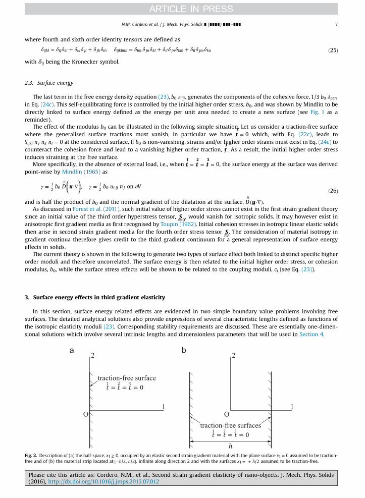
Fig. 2. Description of (a) the half-space, x 01 ≥ , occupied by an elastic second strain gradient material with the plane surface x 01 = assumed to be traction-free and of (b) the material strip located at h h/2, /2[− ], infinite along direction 2 and with the surfaces x h/21 = ± assumed to be traction-free.
Please cite this article as: Cordero, N.M., et al., Second strain gradient elasticity of nano-objects. J. Mech. Phys. Solids(2016), http://dx.doi.org/10.1016/j.jmps.2015.07.012i

N.M. Cordero et al. / J. Mech. Phys. Solids ∎ (∎∎∎∎) ∎∎∎–∎∎∎8
3.1. Half-space with a free surface
The half-space, x 01 ≥ , in a Cartesian coordinate system x x x, ,1 2 3{ } is occupied by an elastic second strain gradient ma-terial as described in Fig. 2.
In continuum mechanics, free surfaces are associated with Neumann conditions of vanishing tractions. In the context of asecond strain gradient theory, the planar surface, x 01 = , is traction-free if
t t t x0 at 0. 271 2 3
1= = = = ( )
We look for displacement fields of the form
u u x u u, 0. 281 1 1 2 3= ( ) = = ( )
The current problem is then essentially one-dimensional. The stress-equation of equilibrium (21) becomes
S S 0 2911,1 111,11 1111,111σ − + = ( )
in the absence of body forces. The boundary conditions (22) then become
S S S S S x0, 0, 0 at 0 3011 111,1 1111,11 111 1111,1 1111 1σ − + = − = = = ( )
as the terms with surface gradients (i.e., with the operators Dtor L) in (22) vanish in the case of the present flat surface. With
the assumed displacement field Equation (28), the potential energy density (23) is a function of the strain components ε11,ε111 and ε1111 only. Thus,
⎛⎝⎜
⎞⎠⎟
⎛⎝⎜
⎞⎠⎟
A Bc b, ,
2 2 2 3111 111 1111 11
21112
11112
11 1111 0 1111ρΨ ε ε ε λ μ ε ε ε ε ε ε= + + + + ¯ +( )
with the following notations for reduced moduli,
A a a a a a B b b b b b b b c c c c2 , 2 , . 321 2 3 4 5 1 2 3 4 5 6 7 1 2 3( ) ( )= + + + + = + + + + + + ¯ = + + ( )
From Table 1, it can be seen that the constants A and c have the dimension of forces (N) and B has the dimension of forcetimes unit surface (N mm2). The material parameters L1 and L2 with the dimension of length are now defined, together withthe dimensionless parameters η and η0:
LA
LBA
cA
bA/2
, , , .331
222
00
λ μη η=
+= =
¯=
( )
The next objective here is to rewrite the potential energy density, Eq. (31), as a function of three dimensionless arguments.Hence,
L L, , , , . 3411 111 1111 11 1 111 22
1111( ) ( )ρΨ ε ε ε ρΨ ε ε ε= ^( )
Note that the local stability of the material behaviour is ensured when the function x y z, ,Ψ ( ) is convex with respect to itsarguments. This implies the following requirements:
Fig. 3. Effects of the material parameters η and L L/22
12: (a) stability requirements; the potential Ψ is convex for the sets of material parameters taken in the
coloured area. (b) Set of l12 and l2
2: the square of the characteristic lengths l1 and l2 can either be complex or real depending on the sign of the part under thesquare root in Eqs. (39) and (40). The coloured area corresponds to the sets of material parameters for which l1
2 and l22 are real. (For interpretation of the
references to colour in this figure caption, the reader is referred to the web version of this paper.)
Please cite this article as: Cordero, N.M., et al., Second strain gradient elasticity of nano-objects. J. Mech. Phys. Solids(2016), http://dx.doi.org/10.1016/j.jmps.2015.07.012i

N.M. Cordero et al. / J. Mech. Phys. Solids ∎ (∎∎∎∎) ∎∎∎–∎∎∎ 9
L LL
L0, 0, 2 .
3512
22 2
2
12
2η≥ ≥ ≥( )
Recalling the expressions of the material parameters (33), these requirements impose that the moduli A and B are positive;however the modulus c can be either positive or negative. These will be used as a guideline to choose physically relevantmaterial parameters for the theory. No condition for the initial higher order stress, b0, arises from the convexity and thismaterial parameter can be calibrated using the expression of the point surface energy given by Eq. (26). The requirements(35) are summarised in Fig. 3(a) where the coloured area represents the values of the material parameters η and L L/2
212,
which lead to a convex potential, Ψ . The chosen notations in Eq. (33) provide a convenient description of the materialparameters: L1 and L2 are related to the first and second strain gradients, respectively, and the ratio L L/2
212 represents their
relative weight, η describes the coupling between strain and the third gradient of displacement.Combining Eqs. (10), (28) and (24), the components s11, S111 and S1111 of the stress tensors are derived:
c2 , 36a11 11 1111( )σ λ μ ε ε= + + ¯ ( )
S A , 36b111 111ε= ( )
S B c b . 36c1111 1111 11 0ε ε= + ¯ + ( )
Substituting these expressions into the stress-equation of equilibrium (29) and recalling that u11 1,1ε = , u111 1,111ε = andu1111 1,111ε = , the following sixth order displacement-equation of equilibrium is derived:
⎛⎝⎜⎜
⎞⎠⎟⎟
⎛⎝⎜⎜
⎞⎠⎟⎟l
ddx
ld
dx
d u
dx1 1 0.
3712
2
12 2
22
12
21
12
− − =( )
It involves new characteristic lengths defined in the same way as in Mindlin (1965), namely,
l lB
l lA c
2,
22
,381
222
12
22
λ μ λ μ=
++ = − ¯
+ ( )
from which the individual intrinsic lengths, l1 and l2, can be obtained:
lA c A c B
lA c A c B2 2 4 2
2 2,
2 2 4 2
2 2,
3912
2
22
2( ) ( )λ μ
λ μ
λ μ
λ μ=
− ¯ + ( − ¯) − +
( + )=
− ¯ − ( − ¯) − +
( + ) ( )
or alternatively:
⎛⎝⎜⎜
⎞⎠⎟⎟
⎛⎝⎜⎜
⎞⎠⎟⎟l
L L
Ll
L L
L41 2 1 2 8 ,
41 2 1 2 8 ,
4012 1
22 2
2
12 2
2 12
2 22
12
η η η η= − + ( − ) − = − − ( − ) −( )
using the previously defined characteristic lengths L1 and L2. The solution of (37) then has the general form:
u x e e e e x . 41x l x l x l x l1 1 1
/2
/3
/4
/5 1 61 1 1 1 1 2 1 2α α α α α α( ) = + + + + + ( )− −
The different types of material responses that can be described by these solutions are now discussed. The characteristiclengths l1 and l2 must be considered as complex numbers. Then, the exponentials e x l/1 1± and e x l/1 2± in the solution of thedisplacement-equation of equilibrium (41) can alternatively correspond to hyperbolic functions if both l1 and l2 are real
Fig. 4. Sign of (a) l12( )R and (b) l2
2( )R : the coloured areas correspond to the sets of material parameters for which the real part of the square of the lengthsl1 and l2 is positive. These results are obtained with L1
2 positive. (For interpretation of the references to colour in this figure caption, the reader is referred tothe web version of this paper.)
Please cite this article as: Cordero, N.M., et al., Second strain gradient elasticity of nano-objects. J. Mech. Phys. Solids(2016), http://dx.doi.org/10.1016/j.jmps.2015.07.012i

Fig. 5. Summary of the four main cases predicted by the theory. Only the sets of material parameters taken in areas “1” and “3” lead to solutions vanishingat infinity. The hatched area represents the convex domain described by the requirements (35). This convex domain is associated with both exponentialand aperiodic physically relevant behaviour (i.e., convex domain 1 3⊂ ∪ ).
N.M. Cordero et al. / J. Mech. Phys. Solids ∎ (∎∎∎∎) ∎∎∎–∎∎∎10
numbers, trigonometric functions if both l1 and l2 are imaginary numbers, or aperiodic functions if both real and imaginaryparts of l1 and l2 are non-zero.
A study of the expressions of these characteristic lengths (39) or (40) is needed to know the form of the solution for agiven set of material parameters and then to fully understand the 1D material behaviour. For that purpose, the sign of thepart A c B2 4 22 ( )λ μ( − ¯) − + or, equivalently, L L1 2 8 /2
22
12η( − ) − under the square root in both expressions (39) and (40) must
be considered: if it is positive, l12 and l2
2 are real; if not, l12 and l2
2 are complex numbers. These two possibilities are representedin Fig. 3(b). Similarly, the sign of the real part of l1
2 and l22, represented in Fig. 4, has a strong impact on the resulting
behaviour. The various cases arising from the combination of the previous conclusions are summarised in Fig. 5:
1. If l12 and l2
2 are real (i.e., l l, 012
22( ) =I ) and if l1
2 and l22 are positive, then l1 and l2 are real and the solution of the dis-
placement-equation of equilibrium (41) becomes
u x e e 42x l x l1 1 2
/4
/1 1 1 2α α( ) = + ( )− −
as the considered case is semi-infinite and therefore requires a solution vanishing at infinity. Eq. (42) is given in the case ofpositive characteristic lengths l1 and l2, the exponentials vanishing at infinity being e x l/1 1− and e x l/1 2− . With negative l1 and l2,the two remaining terms in the solution of the displacement-equation of equilibrium, would be the terms with α1 and α3
with the vanishing exponentials ex l/1 1 and ex l/1 2. Eq. (42) can also be written as
⎡⎣⎢
⎛⎝⎜
⎞⎠⎟
⎛⎝⎜
⎞⎠⎟
⎤⎦⎥
⎡⎣⎢
⎛⎝⎜
⎞⎠⎟
⎛⎝⎜
⎞⎠⎟
⎤⎦⎥u x
xl
xl
xl
xl
cosh sinh cosh sinh .43
1 1 21
1
1
14
1
2
1
2α α( ) = − + −
( )
It describes an exponential decrease of the surface effects as the distance from the traction-free surface increases. This casecorresponds to the area “1” of Fig. 5.2. If l1
2 and l22 are real and if l1
2 and l22 are negative, then l1 and l2 (and consequently, α1, α2, α3 and α4) are imaginary (i.e.,
l l, 01 2( ) =R , l l, 01 2( ) ≠I ) and (41) can be written as
⎪
⎪
⎪
⎪
⎧⎨⎩
⎡⎣⎢
⎛⎝⎜
⎞⎠⎟
⎛⎝⎜
⎞⎠⎟
⎤⎦⎥
⎡⎣⎢
⎛⎝⎜
⎞⎠⎟
⎛⎝⎜
⎞⎠⎟
⎤⎦⎥
⎡⎣⎢
⎛⎝⎜
⎞⎠⎟
⎛⎝⎜
⎞⎠⎟
⎤⎦⎥
⎡⎣⎢
⎛⎝⎜
⎞⎠⎟
⎛⎝⎜
⎞⎠⎟
⎤⎦⎥
⎫⎬⎭
u xixl
iixl
ixl
iixl
ixl
iixl
ixl
iixl
cos sin cos sin
cos sin cos sin ,44a
1 1 11
1
1
12
1
1
1
1
31
2
1
24
1
2
1
2
α α
α α
( ) = − + +
+ − + +( )
R
⎛⎝⎜
⎞⎠⎟
⎛⎝⎜
⎞⎠⎟
⎛⎝⎜
⎞⎠⎟
⎛⎝⎜
⎞⎠⎟
⎛⎝⎜
⎞⎠⎟
⎛⎝⎜
⎞⎠⎟
⎛⎝⎜
⎞⎠⎟
⎛⎝⎜
⎞⎠⎟
u xxl
xl
xl
xl
sin sin sin
sin .44b
1 1 11
12
1
13
1
2
41
2
α α α
α
( ) =( )
−( )
+( )
−( ) ( )
II
II
II
II
This solution, which oscillates, does not vanish at infinity and has no physical meaning for the half-space problem. The setsof material parameters, corresponding to area “2” of Fig. 5, are therefore excluded.
Please cite this article as: Cordero, N.M., et al., Second strain gradient elasticity of nano-objects. J. Mech. Phys. Solids(2016), http://dx.doi.org/10.1016/j.jmps.2015.07.012i

N.M. Cordero et al. / J. Mech. Phys. Solids ∎ (∎∎∎∎) ∎∎∎–∎∎∎ 11
3. If l12 and l2
2 are complex numbers (i.e., l l, 01 2( ) ≠R , l l, 01 2( ) ≠I ), l1 and l2 are complex as well and (41) can be written as
⎡⎣⎢⎢
⎛⎝⎜⎜
⎞⎠⎟⎟
⎛⎝⎜⎜
⎞⎠⎟⎟
⎤⎦⎥⎥
⎡⎣⎢⎢
⎛⎝⎜⎜
⎞⎠⎟⎟
⎛⎝⎜⎜
⎞⎠⎟⎟
⎤⎦⎥⎥
u x ex l
l l
x l
l l
ex l
l l
x l
l l
cos sin
cos sin ,45
x l l l
x l l l
1 1/
21 1
12
12 2
1 1
12
12
/4
1 2
22
22 4
1 2
22
22
1 1 1 2 1 2
1 2 2 2 2 2
α α
α α
( ) = ( )( )
( ) + ( )− ( )
( )( ) + ( )
+ ( )( )
( ) + ( )− ( )
( )( ) + ( ) ( )
− ( ) ( ( ) + ( ) )
− ( ) ( ( ) + ( ) )
RI
R II
I
R I
RI
R II
I
R I
R R I
R R I
with l1( )R and l2( )R being positive, ensuring that u x1 1( ) vanishes at infinity. A similar solution exists with l1( )R and l2( )R
being negative, the remaining terms are then the terms with α1 and α3 of Eq. (41). Here, the oscillating solution decreasesexponentially so that the surface effects remain localised in the traction-free surface region. This case corresponds tomaterial parameters taken in area “3” of Fig. 5.4. The last case corresponds to area “4”. It is obtained with l1
2 and l22 being real and of opposite signs leading to l1 real and l2
imaginary. The solution takes the form of a sum of an exponential and a trigonometric function,
⎛⎝⎜
⎞⎠⎟
⎛⎝⎜
⎞⎠⎟
⎛⎝⎜
⎞⎠⎟
⎛⎝⎜
⎞⎠⎟
u x e exl
xl
xl
xl
cos sin
cos sin ,46
x l x l1 1 1
/2
/3
1
23
1
2
41
24
1
2
1 1 1 1α α α α
α α
( ) = ( ) + ( ) + ( )( )
+ ( )( )
+ ( )( )
− ( )( ) ( )
−R R RI
II
RI
II
and has no physical meaning.
Fig. 5 summarises the four cases just described. As discussed, only the sets of material parameters taken in the areas “1”and “3” lead to physically relevant behaviour. The stability requirements initially presented in Fig. 3(a) are also recalled, thehatched area representing the combination of material parameters leading to a convex potential energy density. This convexdomain is associated with both exponentially decreasing and aperiodic physically relevant behaviour.
In the following, the solution of the displacement-equation of equilibrium is supposed to have the general form given inEq. (42) that is vanishing at infinity. Recalling the discussions made in cases 1 and 3, this implies that l1
2 and l22 or l1( )R and
l2( )R are positive.Successive derivations of u x1 1( ) give the expressions for x11 1ε ( ), x111 1ε ( ) and x1111 1ε ( ). By using the components of the stress
tensors as expressed in Eq. (36), the two last boundary conditions of Eq. (30) become
A c B B c b x0, at 0. 47111 1111,1 1111 11 0 1( )ε ε ε ε− ¯ − = + ¯ = − = ( )
The two unknown constants α2 and α4 in the solution given by Eq. (42) then are
ll l l
l l l l l l
l l l
l l l, ,
48
c
c c
c
c2 0
2 12
22 2
1 22 2 2
2 12 2 2 4 2
22
12 2
12
22 2
( )( ) ( )
( )( )α α α=
+
+ − += −
+
+ ( )
with the new characteristic lengths
lc
L2
12 49c
212
λ μη=
¯+
=( )
and
lb
L2
12
.500
2 00 1
2
λ μη=
+=
( )
These relations clearly show that no surface effect can occur in the absence of initial higher order stress, i.e., when b 00 = .Indeed, if the modulus b0 or its associated dimensionless material parameter η0 related to surface energy vanishes, thecharacteristic length l0 and the constants α2 and α4 vanish as well leading finally to u x 01 1( ) = . Note that this completesolution of the boundary value problem is valid for both physically relevant Cases 1 and 3.
The corresponding displacement, strain and stress profiles close to the traction-free surface are presented in Fig. 6. Theseprofiles are obtained for L 0.3 nm1 = , a fixed ratio L L/ 12
212 = , 0.10η = and for four different values of η. These sets of material
parameters correspond to the first three cases simulated by the theory: 3.0η = − and 1.2η = − belong to the area “1” inFig. 5 and to u1 hyperbolic as in Eq. (43); note that 3.0η = − is not in the convex domain. In the same way, 1.3η = and
1.9η = belong to areas “2” and “3” and to u1 as in Eqs. (44) and (45), respectively. The profiles presented in Fig. 6 show thatthe surface energy effects produced by the theory can either lead to higher or smaller inter-atomic distances close to the freesurface. The free surface and subsurface material can therefore be either in tension or compression. Different possible stressdistributions are represented in Fig. 6(c), together with a schematic representation of the corresponding atomic positionsclose to the surface. The results obtained with these parameters are physically relevant, except for 1.9η = , taken in area “2”,which leads to a spurious oscillating solution. It is remarkable that, within the second strain gradient theory with an initial
Please cite this article as: Cordero, N.M., et al., Second strain gradient elasticity of nano-objects. J. Mech. Phys. Solids(2016), http://dx.doi.org/10.1016/j.jmps.2015.07.012i

a
b
c
Fig. 6. Profiles of (a) the displacement component u1, (b) the strain component ε11 and (c) the stress component s11 close to the traction-free surface (atx 01 = ). Four sets of material parameters are considered: E 140 GPa= , 0.3ν = , L 0.3 nm1 = and a fixed ratio L L/ 12
212 = . The surface energy related parameter
0.10η = and four values of η are used in order to illustrate the four different cases arising in the theory.
Please cite this article as: Cordero, N.M., et al., Second strain gradient elasticity of nano-objects. J. Mech. Phys. Solids(2016), http://dx.doi.org/10.1016/j.jmps.2015.07.012i
N.M. Cordero et al. / J. Mech. Phys. Solids ∎ (∎∎∎∎) ∎∎∎–∎∎∎12
N.M. Cordero et al. / J. Mech. Phys. Solids ∎ (∎∎∎∎) ∎∎∎–∎∎∎ 13
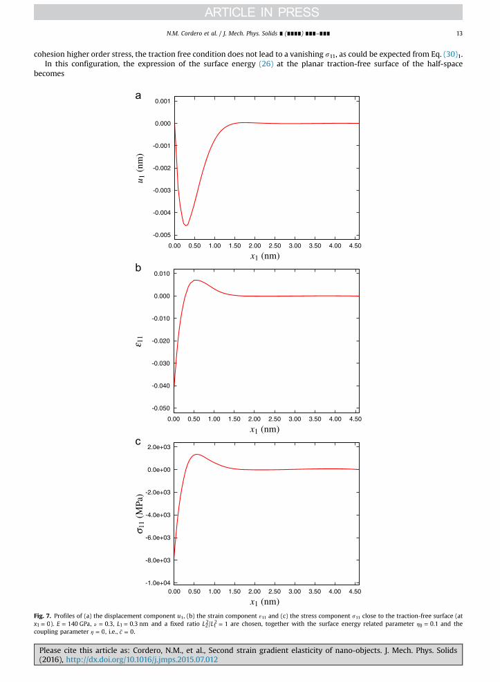
cohesion higher order stress, the traction free condition does not lead to a vanishing s11, as could be expected from Eq. (30)1.In this configuration, the expression of the surface energy (26) at the planar traction-free surface of the half-space
becomes
a
b
c
Fig. 7. Profiles of (a) the displacement component u1, (b) the strain component ε11 and (c) the stress component s11 close to the traction-free surface (atx 01 = ). E 140 GPa= , 0.3ν = , L 0.3 nm1 = and a fixed ratio L L/ 12
212 = are chosen, together with the surface energy related parameter 0.10η = and the
coupling parameter 0η = , i.e., c 0¯ = .
Please cite this article as: Cordero, N.M., et al., Second strain gradient elasticity of nano-objects. J. Mech. Phys. Solids(2016), http://dx.doi.org/10.1016/j.jmps.2015.07.012i
N.M. Cordero et al. / J. Mech. Phys. Solids ∎ (∎∎∎∎) ∎∎∎–∎∎∎14
⎛
⎝⎜⎜⎜
⎞
⎠⎟⎟⎟b b
l l
l l l
l l l l l lx
12
12
12
2at 0.
51c c
0 111 02
12
4
22
04
12
22
1 22 2 2
2 12 2 2 1
( )( )( ) ( )
γ εα α λ μ
= − = − + =+ −
+ − +=
( )
The initial higher order stress, b0 (or alternatively the corresponding dimensionless material parameter, η0), only appears inthe constants α2 and α4 (48) through the characteristic length, l0
2, then it has no effect on the shape of the simulatedbehaviour. However, as suggested by Eq. (51), b0 controls the amplitude of the surface energy.
The effect of the modulus c that enables, in the present case, the coupling between the strain, ε11, and the third gradientof the displacement field, ε1111, is presented and discussed in detail in Section 4. At this point, a first remark can be madefrom the solution of the displacement-equation of equilibrium (42), the expressions of the constants (48) and the expressionof l c/ 2c
2 λ μ= ¯ ( + ). When c 0¯ = , there is no displacement of the traction-free surface and no volume variation even with anon-zero initial higher order stress, b0, i.e., u b0 0,1 0( ) = ∀ . However, displacements of internal material points occur close tothe traction-free surface, i.e., u x 0 01 1( > ) ≠ . This specific case is described in Fig. 7.
3.2. Interaction between two parallel free surfaces
A material strip located at h h/2, /2[− ] and infinite along the lateral directions 2 and 3 is considered, as described in Fig. 2.Both surfaces at x h/21 = ± are assumed to be traction-free:
t t t xh
0 at2
, 521 2 3
1= = = = ± ( )
with h being the plate thickness. The purpose here is to show the interaction of the free surface effects evidenced in theprevious section when the plate becomes very thin. The conditions u u 02 3= = are still enforced so that the problem re-mains one-dimensional. The same resolution steps as in Section 3.1 are then followed so that Eqs. (28)–(40) remain validand lead to a displacement of the same form as in Eq. (41). The two last boundary conditions in Eqs. (30) and (52) now
a
b
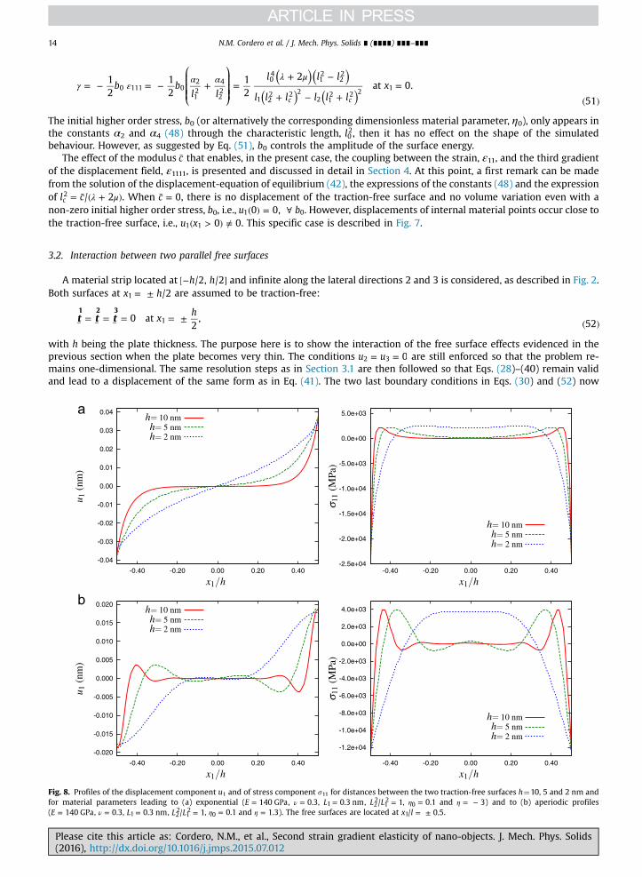
Fig. 8. Profiles of the displacement component u1 and of stress component s11 for distances between the two traction-free surfaces h¼10, 5 and 2 nm andfor material parameters leading to (a) exponential (E 140 GPa= , 0.3ν = , L 0.3 nm1 = , L L/ 12
212 = , 0.10η = and 3η = − ) and to (b) aperiodic profiles
(E 140 GPa= , 0.3ν = , L 0.3 nm1 = , L L/ 122
12 = , 0.10η = and 1.3η = ). The free surfaces are located at x l/ 0.51 = ± .
Please cite this article as: Cordero, N.M., et al., Second strain gradient elasticity of nano-objects. J. Mech. Phys. Solids(2016), http://dx.doi.org/10.1016/j.jmps.2015.07.012i

N.M. Cordero et al. / J. Mech. Phys. Solids ∎ (∎∎∎∎) ∎∎∎–∎∎∎ 15
become
⎛⎝⎜
⎞⎠⎟A c B B c b x
h0, at
2.
53111 1111,1 1111 11 0 1ε ε ε ε− ¯ − = + ¯ = − = ±
( )
Eqs. (53) are used to determine the constants α1 to α6 of the solution (41):
⎪ ⎪
⎪ ⎪⎛
⎝⎜⎜
⎞
⎠⎟⎟
⎧⎨⎩
⎛⎝⎜⎜
⎞⎠⎟⎟
⎡⎣⎢
⎤⎦⎛⎝⎜
⎞⎠⎟
⎛⎝⎜
⎞⎠⎟
⎞⎠⎟⎟
⎫⎬⎭
l l l lhl
l l lhl
l l lhl
12
sinh2
coth2
coth2
,54a
c c c1 02
12
22 2
11 2
2 2 2
12 1
2 2 2
2
1
( ( )α = − + + − +( )
−
, 54b2 1α α= − ( )
⎛
⎝⎜⎜
⎞
⎠⎟⎟
⎛
⎝⎜⎜
⎞
⎠⎟⎟
⎡⎣⎢
⎛⎝⎜
⎞⎠⎟
⎛⎝⎜
⎞⎠⎟
⎤⎦⎥l l l
hl
l l lhl
sinh2
sinh2
,54c
c c3 1 22
12 2
112
22 2
2
1
α α= − + +( )
−
, 54d4 3α α= − ( )
0, 0. 54e5 6α α= = ( )
If h is large compared to l1 and l2, these solutions converge towards the superposition of those solutions for two half-spaceswith free surfaces. When h decreases, the perturbations induced by the free surface effect overlap as illustrated next. Theprofiles of the displacement component u1 and stress component s11 are presented in Fig. 8 for different distances h and forsets of material parameters giving hyperbolic and aperiodic solutions, as discussed in Section 3.1.
The used sets of parameters systematically lead to a thickening of the plate induced by the surface energy effect sinceu h u h/2 0, /2 01 1( ) > ( − ) < in all figures. The shrinking or thickening of the plate is directly related to the sign of b0 via theparameter η0 in l0
2, cf. Eq. (50) and (33). Very large s11 stress values, sometimes exceeding 10 GPa, are found at the freesurfaces. For larger values of h, e.g., h 10 nm= , the profiles close to the free surfaces are the same as in the half-space case,see Fig. 6. When h becomes smaller, the zones affected by the surface energy effects start to overlap and the resultingprofiles are significantly modified. In particular, the strain, ε11, becomes almost homogeneous for very thin plates whereas itis localised close to the free surface for thicker samples. This case appears to be of great interest as it is encountered in nano-sized objects such as nano-wires or nano-porous materials where surfaces are very close to each other.
4. Surface elasticity effect: apparent shear of an infinite strip
Casal (1961, 1963) was the first to theoretically consider the tension of a nano-wire made of an isotropic first straingradient material. He derived the boundary layers' effects at the ends of a beam induced by higher order boundary con-ditions. However, he did not mention the non-homogeneous straining close to a free surface. This is due to the fact that sucheffects cannot arise in isotropic first strain gradient materials. These phenomena akin to surface elasticity are now illustratedfor the second strain gradient continuum.
The purpose of this section is to show how the theory can describe surface effects induced by the coupling between thestrain, ε∼, and the third gradient of the displacement field, ε≈. This coupling is controlled by the moduli ci, as can be seen fromthe constitutive equations (24a) and (24c).
The tension of nano-wires and their apparent elastic properties will be investigated based on finite element simulationsto be presented in Section 5.1. In this section, the notion of apparent elastic property is defined in the context of thirdgradient elasticity. Analytical expressions for the apparent shear modulus are derived for an infinite thin strip subjected toshear.
4.1. Resolution of the boundary value problem
The simple shear of an infinite strip of thickness h is considered as described in Fig. 9. Displacements are prescribed tothe upper and lower surfaces corresponding to simple shear:
u hU
u hU
/22
, /22
. 5510
10( ) = ( − ) = − ( )
These upper and lower surfaces are assumed to be free of higher order tractions, i.e.,
t t xh
0 at2
, 562 3
2= = = ± ( )
In addition, in order to focus exclusively on the surface elasticity effects, no surface energy is considered. In other words, the
Please cite this article as: Cordero, N.M., et al., Second strain gradient elasticity of nano-objects. J. Mech. Phys. Solids(2016), http://dx.doi.org/10.1016/j.jmps.2015.07.012i

Fig. 9. Shear of an infinite strip of thickness h. Dirichlet displacement conditions are applied to the upper and lower surfaces. These surfaces are free ofhigher order tractions.
N.M. Cordero et al. / J. Mech. Phys. Solids ∎ (∎∎∎∎) ∎∎∎–∎∎∎16
initial higher order stress, b0, related to surface energy is taken to be equal to zero. Due to the infinite lateral extension of thestrip, the displacement field takes the form
u u x u u, 0. 571 1 2 2 3= ( ) = = ( )
The stress balance equation (21) becomes
S S 0 5812,2 122,22 1222,222σ − + = ( )
and the two last boundary conditions (22) are
S S S xh
0 at2
. 59122 1222,2 1222 2− = = = ± ( )
Recalling the displacement field (57), then the strain energy density (23) is a function of the strain components ε12, ε122 andε1222:
⎛⎝⎜
⎞⎠⎟
A Bc, ,
2 2 6012 122 1222 12
21222
12222
3 12 1222ρΨ ε ε ε μ ε ε ε ε ε= + + +( )
with the new definitions of reduced moduli A and B superseding (32),
A a a B b b2 , 2 . 613 4 5 6( ) ( )= + = + ( )
In the same way as in Sections 3.1 and 3.2, the following reduced material parameters are introduced:
LA
LBA
cA
, , ,621
222 3
μη= = =
( )
which are used to express the potential energy density (60) as a function of dimensionless arguments:
L L, , , , . 6312 122 1222 12 1 122 22
1222( ) ( )ρΨ ε ε ε ρΨ ε ε ε= ^( )
The following requirements can then be obtained based on the convexity of the strain energy potential,
L LL
L0, 0, 2 .
6412
22 2
2
12
2η≥ ≥ ≥( )
This implies that the moduli A and B must be positive while c3 can be either positive or negative. The components s12, S122and S1222 of the stress tensors are obtained from Eqs. (60), (10) and (24):
c2 , 65a12 12 3 1222σ μ ε ε= + ( )
S A , 65b122 122ε= ( )
S B c . 65c1222 1222 3 12ε ε= + ( )
Substituting these expressions into the stress-equation of equilibrium (58) and recalling that u1/212 1,2ε = , u1/2122 1,22ε =and u1/21222 1,222ε = , the following displacement-equation for equilibrium is obtained:
⎛⎝⎜⎜
⎞⎠⎟⎟
⎛⎝⎜⎜
⎞⎠⎟⎟l
ddx
ld
dx
d u
dx1 1 0.
6612
2
22 2
22
22
21
22
− − =( )
The relationships,
Please cite this article as: Cordero, N.M., et al., Second strain gradient elasticity of nano-objects. J. Mech. Phys. Solids(2016), http://dx.doi.org/10.1016/j.jmps.2015.07.012i

N.M. Cordero et al. / J. Mech. Phys. Solids ∎ (∎∎∎∎) ∎∎∎–∎∎∎ 17
l lB
l lA c
2,
22
,671
222
12
22 3
μ μ= + =
−( )
are derived and lead to the following expressions for the lengths l1 and l2:
lA c A c B
lA c A c B2 2 8
4,
2 2 8
4,
6812 3 3
2
22 3 3
2( ) ( )μμ
μμ
=− + − −
=− − − −
( )
or alternatively:
⎛⎝⎜⎜
⎞⎠⎟⎟
⎛⎝⎜⎜
⎞⎠⎟⎟l
L L
Ll
L L
L41 2 1 2 8 ,
41 2 1 2 8 .
6912 1
22 2
2
12 2
2 12
2 22
12
η η η η= − + ( − ) − = − − ( − ) −( )
It can be noted that the chosen notations for the material parameters L1, L2 and η lead to the same expressions of thestability requirements (35) and of the characteristic lengths (40) as in Sections 3.1 and 3.2.
The solution of Eq. (66) takes the form
u x e e e e x , 70x l x l x l x l1 2 1
/2
/3
/4
/5 2 62 1 2 1 2 2 2 2α α α α α α( ) = + + + + + ( )− −
and the boundary conditions (59) require that
⎛⎝⎜
⎞⎠⎟A c B B c x
h0, 0 at
2,
713 122 1222,2 1222 3 12 2ε ε ε ε− − = + = = ±
( )
They are used to find the expressions of the constants α1 to α6:
⎪
⎪
⎛
⎝⎜⎜⎜
⎞
⎠⎟⎟⎟
⎧⎨⎪⎩⎪
⎛⎝⎜⎜
⎞⎠⎟⎟
⎡⎣⎢⎢
⎛⎝⎜⎜
⎞⎠⎟⎟
⎛⎝⎜⎜
⎛⎝⎜
⎞⎠⎟
⎛⎝⎜
⎞⎠⎟
⎞⎠⎟⎟
⎤⎦⎥⎥
⎫⎬⎭
U l l l lhl
l l l h l l lhl
l l lhl
sinh2
4 2 coth2
coth2
,72a
c c c c
c
1 02
12
22 2
1
412
22
1 22 2 2
1
2 12 2 2
2
1
( )
( )
α = + − − +
− +( )
−
, 72b2 1α α= − ( )
⎛
⎝⎜⎜
⎞
⎠⎟⎟
⎛
⎝⎜⎜
⎞
⎠⎟⎟
⎡⎣⎢
⎛⎝⎜
⎞⎠⎟
⎛⎝⎜
⎞⎠⎟
⎤⎦⎥l l l
hl
l l lhl
sinh2
sinh2
,72c
c c3 1 22
12 2
112
22 2
2
1
α α= − + +( )
−
, 72d4 3α α= − ( )
⎛⎝⎜⎜
⎞⎠⎟⎟
⎡⎣⎢
⎛⎝⎜
⎞⎠⎟
⎛⎝⎜
⎞⎠⎟
⎤⎦⎥
⎡⎣ ⎤⎦hl
l l lhl
l l lhl
l l l l2 sinh2
coth2
coth2
,72e
c c c c5 11
1 22 2 2
12 1
2 2 2
2
212
22 2 1( ) ( ) ( )α α= − + − + +
( )
−
0, 72f6α = ( )
with the new characteristic length,
lc
L2
12
.73c
2 312
μη= =
( )
Recall that the initial higher order stress, b0, and its related characteristic length, l02, do not appear in these expressions as the
surface energy is purposely not considered in the present case. Examination of Eqs. (72) shows that surface effects onlyoccur if a coupling exists between the component of the strain ε12 and the component of the third gradient of thedisplacement field ε1222. If the coupling modulus c 03 = , then lc¼0, 01 2 3 4α α α α= = = = and U h/5 0α = . The standardhomogeneous shear solution is retrieved: u x U x h/1 2 0 2( ) = .
The same remark can be made on the imposed displacement at the upper and lower surfaces. Indeed, if U 00 = , all theconstants αi in Eq. (70) vanish and then u x 01 2( ) = . This would not be the case in the presence of surface energy since, asshown is Section 3.1, surface and subsurface straining arises even in the absence of external loading at traction-free surfaces.
The profiles of the displacement component u1 and of stress component s12 are shown in Fig. 10 for various thicknesses hof the strip and for sets of material parameters leading to physically acceptable hyperbolic and aperiodic solutions. Thisfigure shows that for larger thicknesses h of the strip, the profiles are almost linear and close to the solution for a classicalcontinuum. The surface and subsurface elasticity effects are found to be localised at the upper and lower surfaces, and the
Please cite this article as: Cordero, N.M., et al., Second strain gradient elasticity of nano-objects. J. Mech. Phys. Solids(2016), http://dx.doi.org/10.1016/j.jmps.2015.07.012i

a
b
Fig. 10. Profiles of the displacement component u1 and of stress component s12 for thicknesses of the infinite strip, h¼50, 10 and 5 nm, and for materialparameters leading to (a) exponential (E 140 GPa= , 0.3ν = , L 0.3 nm1 = , L L/ 12
212 = and 3η = − ) and to (b) aperiodic profiles (E 140 GPa= , 0.3ν = ,
L 0.3 nm1 = , L L/ 122
12 = and 1.3η = ). In both cases, the surface energy is not considered, i.e., b 00 0η= = .
N.M. Cordero et al. / J. Mech. Phys. Solids ∎ (∎∎∎∎) ∎∎∎–∎∎∎18
affected zones remain small compared to the thickness h. These surface effects become stronger when the strip gets thinner,i.e., when the higher order traction-free surfaces get closer to each other.
4.2. Determination of the apparent shear modulus
Experimental measurements of apparent elastic properties of nano-objects are based on the ratio of effective stress andstrain properties, since the direct measurement of higher order stresses remains an open question. Such apparent quantitiescan be derived from the previous theory by proper averaging procedures.
The apparent shear modulus μapp is defined by averaging the stress component, s12, and the strain component, ε12, alongthe thickness of the infinite strip as
dx dx2 .74h
happ
h
h
/2
/212 2
/2
/212 2∫ ∫σ μ ε=
( )− −
The following expression of the apparent shear modulus is then obtained from the analytical solution of Section 4.1:
⎛⎝⎜
⎞⎠⎟
⎛⎝⎜
⎞⎠⎟
⎛⎝⎜
⎞⎠⎟
⎛⎝⎜
⎞⎠⎟
⎛⎝⎜
⎞⎠⎟
l l lhl
l l lhl
l l lhl
l l lhl h
l l l
coth2
coth2
coth2
coth2
2.
75
appc c
c c c
1 22 2 2
12 1
2 2 2
2
1 22 2 2
12 1
2 2 2
2
412
22
( ) ( )
( ) ( )μ μ=
+ − +
+ − + − −( )
or, equivalently,
Please cite this article as: Cordero, N.M., et al., Second strain gradient elasticity of nano-objects. J. Mech. Phys. Solids(2016), http://dx.doi.org/10.1016/j.jmps.2015.07.012i

Fig. 11. Effect of the thickness of the infinite strip, h, on the evolution of the apparent shear modulus, μapp, for E 140 GPa= , 0.3ν = , L 0.3 nm1 = , L L/ 122
12 =
and for two different values of the coupling parameter, η. The horizontal line corresponds to the classical solution obtained without coupling ( 0η = ), orequivalently, without surface stress effects. Note that in all of these cases, the surface energy is not considered, i.e., b 00 0η= = .
N.M. Cordero et al. / J. Mech. Phys. Solids ∎ (∎∎∎∎) ∎∎∎–∎∎∎ 19
⎛⎝⎜
⎞⎠⎟
⎛⎝⎜
⎞⎠⎟
h
l l l
l l lhl
l l lhl
12
coth2
coth2
.
76
app
c
c c
412
22
1 22 2 2
12 1
2 2 2
2
( )( ) ( )
μμ
= −−
+ − +( )
It is apparent in this relation that μapp is size-dependent, the effect of the thickness h on its value is plotted for different setsof material parameters in Fig. 11. For large values of h, the surface elasticity effects are negligible and the bulk shear modulusμ is retrieved,
lim . 77h
appμ μ= ( )→∞
When the strip thickness decreases, the apparent elastic property progressively departs from one of the bulk and tends tothe limit
⎛⎝⎜⎜
⎞⎠⎟⎟l
l llim 1 .
78h
app c
0
4
12
22
μ μ= −( )→
Note that when the coupling modulus, c3, or equivalently the characteristic length, lc, vanishes, the ratio /appμ μ is equal toone and no surface elasticity effect arises. Fig. 11 shows that the apparent shear modulus, μapp, can either increase ordecrease for smaller h. This only depends on the material parameter related to the coupling, namely η controlling the sign ofl1
2 and l22 according to (68). In this figure, the horizontal line corresponds to the classical solution obtained without surface
elasticity effects. The same dependency appears in the limit presented in Eq. (78). The positivity of the limit apparent shearmodulus given by Eq. (78), and therefore the local stability of the material under shear, is ensured whenl l l L L L2 /4 0c1
222 4
12
22 2
12η− = ( − ) > which is equivalent to the already stated stability condition (64). When both l1
2 and l22 are
positive the nano-scale apparent shear modulus is lower than the bulk one. The values of l12 and l2
2 can be of distinct sign,one being positive, the other one negative, for some negative values of η. This situation leads to a stiffening effect at nano-scale as shown in Fig. 11. However, the stability conditions (64) require l l L L /21
222
12
22= be positive. As a result, shear stiffening
cannot occur in the locally stable regime. This statement is however limited to the boundary value problem considered inthis section, namely a simple shear test with vanishing higher order tractions at the lower and upper boundaries, see Fig. 9.
Some specific cases can be investigated to fully understand the surface stress effects. For example, if l l1 2= (i.e.,L L1 2 8 /2
22
12η( − ) = ), no effect is produced and then
. 79l lapp1 2
μ μ= ( )( = )
This is the specific case of the double root of the differential equation (66). It corresponds to the parabola of Fig. 3(b) separating the two domains in which l1
2 and l22 are real or complex. Moreover, if the generalised modulus related to the
second strain gradient, B, vanishes, we have L 02 → , l 02 → and finally
⎛⎝⎜
⎞⎠⎟
⎛⎝⎜
⎞⎠⎟
hhl
hhl
l
limcoth
2
coth2
2.
80
B
app
0
1
11
μ μ=−
( )
→
Please cite this article as: Cordero, N.M., et al., Second strain gradient elasticity of nano-objects. J. Mech. Phys. Solids(2016), http://dx.doi.org/10.1016/j.jmps.2015.07.012i

N.M. Cordero et al. / J. Mech. Phys. Solids ∎ (∎∎∎∎) ∎∎∎–∎∎∎20
This means that the theory generates size-dependent surface stress effects even if B vanishes. This confirms the fact that, asmentioned before, the surface stress effects predicted by the second strain gradient theory solely depend on the couplingparameter between the strain component, ε12, and the third gradient of the displacement field component, ε1222.
5. Application to the static elastic behaviour of nano-objects
Now that the capabilities of the theory and, more particularly, the generated surface effects, have been demonstrated,more realistic and complex boundary value problems will be considered. They are performed by means of finite elementsimulations making use of the constrained generalised micromorphic approach proposed by Germain (1973b), Forest(2009), and Forest et al. (2011).
5.1. Apparent tensile elastic behaviour of second strain gradient nano-films
The size-dependent tensile behaviour of nano-objects, especially nano-wires, has been widely investigated due to theirkey role in nano-electromechanical systems (NEMS) (Thomas et al., 2011; Craighead, 2000; Feng et al., 2007; Sanii andAshby, 2010). In particular, their size-dependent elastic properties are studied experimentally using various methods (see,for example, Agrawal et al., 2008; McDowell et al., 2008; Sadeghian et al., 2009). Nano-wires exhibit a very high surface areato volume ratio and therefore their behaviour is strongly affected by surface effects. Using the previous results as a guidelineto define the material parameters, the overall behaviour of such nano-objects and especially the local strain fields arestudied using finite element simulations. To that purpose, the second gradient of strain theory presented in Section 2 isimplemented using the second order micromorphic approach formulated in Appendix A. The micromorphic model isconstrained through the moduli Ha
χ and Hbχ in Eqs. (96) to be as close as possible to the gradient theory. In what follows, Ha
χand Hb
χ are taken sufficiently high to ensure this internal constraint. The main features of the finite element implementationare given in Appendix B. Isoparametric quadratic elements with reduced integration are used.
The boundary value problem solved by means of the finite element method is depicted in Fig. 12(a). Here, a long platewith thickness, d, is subjected to prescribed displacement u U2 = at the top in the direction 2 and fixed displacement u2 atthe bottom. Plane strain conditions are enforced, i.e. u 03 = . Periodicity conditions are imposed to the additional micro-deformation degrees of freedom, between the top and bottom surfaces. The lateral surfaces x d/21 = ± are traction-free atany order, meaning that
t t t xh
0 at2
, 811 2 3
1= = = = ± ( )
at the vertical sides of the 2D geometry presented in Fig. 12(a). In these conditions, the nano-films can be considered ofinfinite length and finite width, d.
Tensile tests on thin films with various thicknesses, d, are simulated in that way. In these tests, the nano-objects areassumed to remain elastic. The contour plots of Fig. 12(b) and the corresponding profiles across the thickness in Fig. 12(c) describe the simulated fields of the lateral strain and axial stress components, ε11 and s22, obtained for three thicknessesand with the material parameters given in Table 2. These parameters are presented using the notation (33) introduced inSection 3 and the corresponding generalised moduli A, B, ci and b0 are also given. The coupling moduli ci′ used in themicromorphic model are defined using the equivalences between ci and ci′, see Eq. (108). The results given in Fig. 12 revealthat the surface stress effects are localised at the surface of the larger film of thickness d 50 nm= . The fields and profiles ofε11 and s22 are then close to those that can be obtained with a classical continuum. However, for smaller d, the surface stresseffects become more significant and the affected zone spreads across the thickness. These results agree with the previousobservations made in the infinite strip shear case.
Recalling that plane strain conditions are used, the apparent Poisson ratio, νapp, and the apparent Young modulus, Eapp,are calculated as
82app 11
11 22ν
εε ε
=− ( )
and
E1
,83
appapp
22
22
2σ νε
=( − )
( )
where the macroscopic strains and stress ε11, ε22 and s22 are computed from the finite element simulations by averaging thecorresponding quantities over the whole sample. These apparent elastic constants are found to be size-dependent. Fig. 13shows the effect of the film thickness, d, on the evolution of the apparent Young modulus, Eapp, for the material parametersgiven in Table 2. These parameters were identified in order to reproduce, as quantitatively as possible, the size-dependentbehaviour of ZnO nano-wires for which experimental data is available (Agrawal et al., 2008). In the experiment, tensile testswere performed on single crystal ZnO nano-wires having a [0001] oriented wurtzite structure. It must be noted that the real
Please cite this article as: Cordero, N.M., et al., Second strain gradient elasticity of nano-objects. J. Mech. Phys. Solids(2016), http://dx.doi.org/10.1016/j.jmps.2015.07.012i
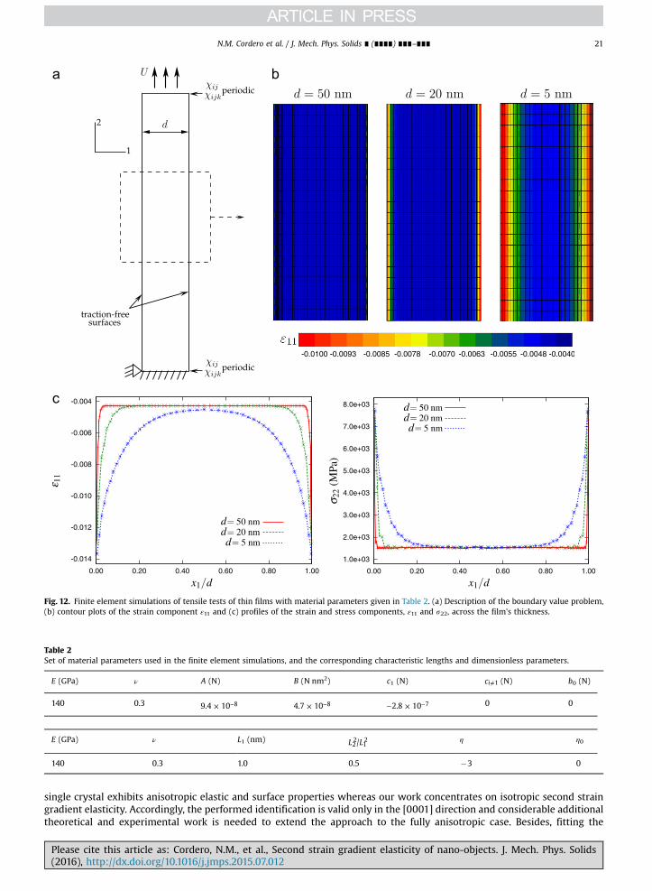
Table 2Set of material parameters used in the finite element simulations, and the corresponding characteristic lengths and dimensionless parameters.
E (GPa) ν A (N) B (N nm2) c1 (N) ci 1≠ (N) b0 (N)
140 0.3 9.4 10 8× − 4.7 10 8× − 2.8 10 7− × − 0 0
E (GPa) ν L1 (nm) L L/22
12 η η0
140 0.3 1.0 0.5 �3 0
Fig. 12. Finite element simulations of tensile tests of thin films with material parameters given in Table 2. (a) Description of the boundary value problem,(b) contour plots of the strain component ε11 and (c) profiles of the strain and stress components, ε11 and s22, across the film's thickness.
N.M. Cordero et al. / J. Mech. Phys. Solids ∎ (∎∎∎∎) ∎∎∎–∎∎∎ 21
single crystal exhibits anisotropic elastic and surface properties whereas our work concentrates on isotropic second straingradient elasticity. Accordingly, the performed identification is valid only in the [0001] direction and considerable additionaltheoretical and experimental work is needed to extend the approach to the fully anisotropic case. Besides, fitting the
Please cite this article as: Cordero, N.M., et al., Second strain gradient elasticity of nano-objects. J. Mech. Phys. Solids(2016), http://dx.doi.org/10.1016/j.jmps.2015.07.012i

Fig. 13. Effect of the nano-film thickness, d, on the evolution of the apparent Young modulus, Eapp, for the material parameters given in Table 2. Thehorizontal line corresponds to the classical solution obtained without surface effects or equivalently to the bulk Young modulus. The plotted experimentaldata come from Agrawal et al. (2008) and are obtained with tensile tests of single crystal ZnO nano-wires having a [0001] oriented wurtzite structure.
N.M. Cordero et al. / J. Mech. Phys. Solids ∎ (∎∎∎∎) ∎∎∎–∎∎∎22
simulation results for nano-plates to the experimental results for nano-wires can only lead to tentative and qualitativevalues of the corresponding moduli. The identification was performed using the results from the previous sections as aguideline. Indeed, the value of the material parameter related to the coupling is first set at 3η = − because it provides arealistic order of magnitude of surface displacement but, unfortunately no experimental information is available for theapparent Poisson ratio. Then, the only dimensional parameter, L1, is calibrated to obtain a size dependent zone for a range ofthicknesses that correspond to the experimental results. Finally, the ratio L L/2 1 is calibrated to refine the fitting. Theidentified material parameters are of the same order of magnitude as those used in the simple cases treated earlier in thispaper. The experimental results are far too scattered and not numerous enough to identify a unique set of materialparameters. The chosen parameters provide sensible results, though probably exaggerated since the actual size effects mayarise at smaller length scales than 100 nm predicted by the model in Fig. 13. A more accurate identification is possible bymeans of molecular dynamics or ab initio simulations. However, large uncertainties remain also with this method becausethe confidence on higher order moduli predicted by such discrete methods is necessarily very limited.
It turns out that the chosen material parameters η, L1, L2 fall in the non-convex domain delimited in Section 3. Althoughno complete identification of the material parameters was possible due to the limited amount of information available forZnO, the exploration of the parameter space lead us to non-positive definite higher order moduli to reproduce the quali-tative increase of the apparent Young modulus for nano-sizes. This finding should be related to the identification of negativefirst strain gradient higher order elastic moduli sometimes found by comparison with the results of atomistic simulations,see Maranganti and Sharma (2007). Negative surface elasticity properties were also found in the context of bulk conven-tional elasticity with energetic and elastic surfaces, see Yvonnet et al. (2008). This question is discussed by Javili et al. (2012)who show mesh dependent finite element simulation results when using negative surface elasticity with a bulk stableelastic substrate. The relevance of the proposed parameters and the possible need for higher order regularisation remainopen questions which require a thorough analysis of the well-posedness of the associated variational problem.
In the same way, Fig. 14 shows the effect of d on the evolution of the apparent Poisson ratio, νapp. A strong enhancementof the apparent Poisson ratio is found for thicknesses less than 20 nm. It is remarkable that the apparent Poisson ratio isfound to tend toward 0.5 in the performed simulations for vanishingly small thicknesses.
The second gradient of strain theory presented in Section 2 is thus able to account, at least qualitatively, for the size-dependent elastic properties of nano-objects. Their mechanical behaviour is affected by surface effects that occur in asurface region of a few nanometers. The obtained results show that these surface effects can be neglected when thethickness is equal to some tens of nanometers or larger. For such sizes, the elastic properties of the bulk material areretrieved.
5.2. Free surface effects in periodic porous nano-structures
Nano-porous materials arouse a strong interest for catalysis and the storage of hydrogen or CO2 wastes due to theiroutstanding surface to volume ratio (Thomas et al., 2011). The surface effect induced by surface energy and surface elasticitycan have a strong impact on the macroscopic behaviour depending on the void volume fraction. Effective mechanicalproperties can be determined based on generalised homogenisation methods. For instance, the effective first displacementgradient theory was identified from the atomic potentials for nano-porous silicon by Magoariec and Danescu (2009). Lattice
Please cite this article as: Cordero, N.M., et al., Second strain gradient elasticity of nano-objects. J. Mech. Phys. Solids(2016), http://dx.doi.org/10.1016/j.jmps.2015.07.012i
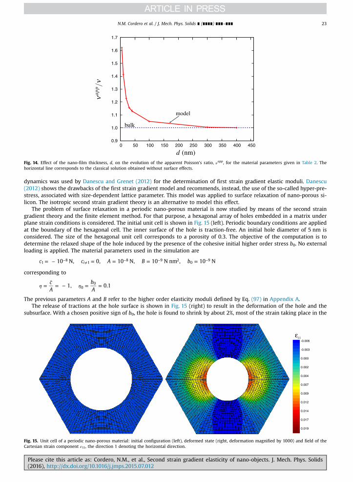
Fig. 14. Effect of the nano-film thickness, d, on the evolution of the apparent Poisson's ratio, νapp, for the material parameters given in Table 2. Thehorizontal line corresponds to the classical solution obtained without surface effects.
N.M. Cordero et al. / J. Mech. Phys. Solids ∎ (∎∎∎∎) ∎∎∎–∎∎∎ 23
dynamics was used by Danescu and Grenet (2012) for the determination of first strain gradient elastic moduli. Danescu(2012) shows the drawbacks of the first strain gradient model and recommends, instead, the use of the so-called hyper-pre-stress, associated with size-dependent lattice parameter. This model was applied to surface relaxation of nano-porous si-licon. The isotropic second strain gradient theory is an alternative to model this effect.
The problem of surface relaxation in a periodic nano-porous material is now studied by means of the second straingradient theory and the finite element method. For that purpose, a hexagonal array of holes embedded in a matrix underplane strain conditions is considered. The initial unit cell is shown in Fig. 15 (left). Periodic boundary conditions are appliedat the boundary of the hexagonal cell. The inner surface of the hole is traction-free. An initial hole diameter of 5 nm isconsidered. The size of the hexagonal unit cell corresponds to a porosity of 0.3. The objective of the computation is todetermine the relaxed shape of the hole induced by the presence of the cohesive initial higher order stress b0. No externalloading is applied. The material parameters used in the simulation are
c c A B b10 N, 0, 10 N, 10 N nm , 10 Ni18
18 9 2
09= − = = = =−
≠− − −
corresponding to
cA
bA
1, 0.100η η=
¯= − = =
The previous parameters A and B refer to the higher order elasticity moduli defined by Eq. (97) in Appendix A.The release of tractions at the hole surface is shown in Fig. 15 (right) to result in the deformation of the hole and the
subsurface. With a chosen positive sign of b0, the hole is found to shrink by about 2%, most of the strain taking place in the
Fig. 15. Unit cell of a periodic nano-porous material: initial configuration (left), deformed state (right, deformation magnified by 1000) and field of theCartesian strain component ε11, the direction 1 denoting the horizontal direction.
Please cite this article as: Cordero, N.M., et al., Second strain gradient elasticity of nano-objects. J. Mech. Phys. Solids(2016), http://dx.doi.org/10.1016/j.jmps.2015.07.012i

N.M. Cordero et al. / J. Mech. Phys. Solids ∎ (∎∎∎∎) ∎∎∎–∎∎∎24
first row of elements around the hole. In the periodic system, holes are close enough for the strained regions around thehole to overlap. This kind of computation can be used to identify the value of the material parameter b0 from the measureddistribution of hole size changes and lattice distortion around holes in nano-porous materials. Note that such measurementsare rendered more difficult by the fact that the surface of nano-porous materials generally is contaminated by externalchemical elements like hydrogen, especially in the case of percolating nano-porosity and hydrogen storage in suchmaterials.
)
6. Conclusions
The main contributions of the present work to the second strain gradient modelling of the elastic behaviour of nano-objects are the following:
� A clear distinction was made between the features of the model responsible for free surface relaxation effects and puresurface elasticity arising during the straining of nano-objects. The surface energy property of the medium is directlyrelated to the initial higher order stress, or cohesion modulus, b0, while the apparent surface stress effects are induced bythe coupling moduli, ci, in the elastic potential (23). They are uncorrelated in the sense that surface elasticity effects canarise for vanishing b0, and vice versa.
� A thorough analysis of a one-dimensional case was presented for the deformation close to a traction free surface in a half-space and in a free-standing film. Decaying, aperiodic and oscillating modes were distinguished in terms of the values ofthe higher order elastic moduli taking stability requirements into account, something which was not done in earliercontributions on the topic.
� The role of the coupling moduli in the modification of apparent elastic properties was highlighted for the first time, bymeans of analytical and numerical solutions in tension and shear of thin strips. This role is apparent in the followingsimple one-dimensional elasticity relation which came out in this work:
c2 8411 11 11,11σ λ μ ε ε= ( + ) + ¯ (
This relation connects the simple stress components, s11, to the second derivative of the strain.� The derived analytical expression (75) of the apparent shear modulus of a material strip under shear clearly shows that
the second strain gradient theory is necessary to model size-dependent apparent shear properties in isotropic media. Inparticular, the first strain gradient theory is not sufficient for that purpose, which settles the existing debate of therequired order of the theory for the gradient continuum modelling of nano-elastic effects. This statement is howeverlimited to the isotropic case.
� Finite Element simulations of second strain gradient elasticity, based on the second order micromorphic continuum withinternal constraints, were performed for the first time. The inhomogeneous strain distribution close to free surfaces in astrip in tension was simulated as a function of plate thickness. The model was also used for the simulation of surfacerelaxation induced by the cohesion hyperstress b0 in an elastic matrix containing a periodic distribution of nano-pores.
� Some of the material parameters of the model were estimated from the size-dependent apparent moduli of ZnO nano-wires in tension. This represents a first step towards systematic identification of higher order elastic moduli from ex-perimental testing on nano-objects, or, possibly from complementary atomistic simulations.
This work represents a contribution to the use of higher grade continuum theories for the modelling of nano-elasticity.The approach has the advantage that it does not geometrically distinguish a boundary region from the bulk. Instead,boundary layers naturally arise from the extra-boundary conditions associated with higher grade continuum theories.
The main limitation of the work is the restriction to the isotropic case highlighting the main features of second straingradient elasticity. Most crystalline nano-objects display an anisotropic material response. Mindlin's second strain gradienttheory must now be extended to the anisotropic case which involves a large number of higher order elastic moduli. Thesymmetry classes and corresponding independent elastic moduli were recently determined for 6-th order tensors arising infirst strain gradient elasticity, see Auffray et al. (2013b), Olive and Auffray (2014), and Auffray (2014). The mathematical toolspresented in the latter references can be used to extend these representations to the 8th order tensor of elastic moduliarising in the second strain gradient model, together with odd-order coupling tensors.
The systematic identification of such a huge number of material parameters represents a major task in future devel-opments of the approach. They can be determined for instance from the effective size-dependent apparent elastic propertiesof nano-porous materials, but also frommolecular dynamics or ab initio results (Villain et al., 2004; Maranganti and Sharma,2007; Yvonnet et al., 2012).
Non-positive definite higher order moduli were found to be necessary to obtain stiffer properties both in shear and planestrain tension. This contributes to the debate on the identification of non-positive higher order or surface elasticity prop-erties sometimes found from atomistic simulations, as discussed by Maranganti and Sharma (2007), Yvonnet et al. (2008),and Javili et al. (2012). The relevance of the proposed parameters and the possible need for higher order regularisationremain open questions which require a thorough analysis of the well-posedness of the associated variational problem.
Please cite this article as: Cordero, N.M., et al., Second strain gradient elasticity of nano-objects. J. Mech. Phys. Solids(2016), http://dx.doi.org/10.1016/j.jmps.2015.07.012i

N.M. Cordero et al. / J. Mech. Phys. Solids ∎ (∎∎∎∎) ∎∎∎–∎∎∎ 25
Global stability of nano-object undergoing oscillating straining modes should be investigated.The links between surface elasticity theory in the spirit of the Gurtin–Murdoch model and second strain gradient
elasticity remain to be established more precisely. For that purpose, it is anticipated that an asymptotic analysis of thesecond strain gradient model close to a free or loaded surface can be performed to identify the surface properties of anequivalent generalised surface model from the bulk higher order elasticity moduli. Such an asymptotic analysis may evenprovide new surface properties not yet accounted for in the existing surface models. Further developments also include theconsideration of elasticity with defects and interfaces (Upadhyay et al., 2012; Dingreville et al., 2014).
Acknowledgments
This work is part of the NANOCRYSTAL Project ANR-07-BLAN-0186. Financial support of ANR is gratefully acknowledged.
Appendix A. Formulation of the second order micromorphic model
This section gives the main equations of the micromorphic approach used for a numerical implementation of the secondgradient of strain theory presented in Section 2. The second order micromorphic approach is formulated following Ger-main's general micromorphic theory introduced for the first time in Germain (1973b). First, its balance and constitutiveequations are given. Then, internal constraints are enforced to control the micro-deformations and obtain the second straingradient theory as a special case of the second order micromorphic model.
A.1. Balance equations
Two micro-deformation variables, χand χ
, are introduced for each material point as second-rank and third-rank tensors
respectively in which the following symmetry properties are considered:
, . 85ij ji ijk jikχ χ χ χ= = ( )
χis called the microstrain tensor. The degrees of freedom of each material point are
uDOF u, , , , , , 86i ij ijk{ } { }χ χ χ χ≔ ( )
where the components of χand χ
are introduced as independent degrees of freedom in addition to the usual displacement
vector. In 2D (plane strain), with the symmetry properties (85), nine degrees of freedom are introduced in addition to the2 displacement components, ui. This number reaches twenty-four in 3D. Following Germain, the generalised power ofinternal forces is a linear form with respect to the degrees of freedom and their first gradient:
s S s Sp
p s S s S
: : :: ,
87
i
iij ij ij ij ij ijk ij k ijk ij k ijk ijkl ijk l, , ,
( ) ( ) ( ) ( )( ) ( )
≈σ ε ε χ χ χ χ χ
σ ε ε χ χ χ χ χ
= + − + ⋮ ⊗ ∇ + ⋮ ⊗ ∇ − + ⊗ ∇
= + − + + − + ( )
∼ ∼ ∼ ∼∼∼( )
( )
Here, σ∼, S∼ and S≈ are the simple, double and triple stress tensors, respectively. Relative stress tensors s∼ and s∼ are introducedas reactions to the difference of strain and microstrain, and of third order microdeformation and the gradient of microstrain.The power of internal forces in a domain V, with smooth boundary V∂ , is then
⎜ ⎟
⎡⎣⎢
⎤⎦⎥
⎡⎣ ⎤⎦ ⎡⎣ ⎤⎦⎡⎣⎢
⎤⎦⎥
⎛⎝
⎞⎠
s S s S
s u s S s s S
n s u S s S
t u t t
p dV
dV
dV
dS
dS
: : ::
. . . : .
. . :
. : ,88a
iV
i
V
V
V
V
{ }( ) ( ) ( ) ( )
( )( ) ( )
( )
∫∫
∫
∫
∫
( )≈
≈
≈
σ ε ε χ χ χ χ χ
σ χ χ
σ χ χ
χ χ
=
= + − + ⋮ ⊗ ∇ + ⋮ ⊗ ∇ − + ⊗ ∇
= − + ∇ + + + ∇ + + ∇ ⋮
+ + + + + ⋮
= + ∼ + ∼ ⋮ ( )
∼ ∼ ∼ ∼
∼ ∼ ∼ ∼
∼ ∼
∼
∼
∼
∼
∼
∼
( ) ( )
∂
∂
Please cite this article as: Cordero, N.M., et al., Second strain gradient elasticity of nano-objects. J. Mech. Phys. Solids(2016), http://dx.doi.org/10.1016/j.jmps.2015.07.012i
N.M. Cordero et al. / J. Mech. Phys. Solids ∎ (∎∎∎∎) ∎∎∎–∎∎∎26
⎜ ⎟ ⎜ ⎟
⎡⎣⎢
⎤⎦⎥
⎡⎣⎢
⎛⎝
⎞⎠
⎛⎝
⎞⎠
⎤⎦⎥
⎡⎣⎢
⎤⎦⎥
⎛⎝⎜
⎞⎠⎟
s S s S dV
s u s S s s S dV
s n u S s n S n dS
t u t t dS.88b
iV
ij ij ij ij ij ijk ij k ijk ij k ijk ijkl ijk l
Vij ij j i ij ijk ijk k ij ijk ijkl l ijk
Vij ij j i ijk ijk k ij ijkl l ijk
Vi i ij ij ijk ijk
, , ,
, , ,
( ) ( )
( ) ( )( ) ( )
∫
∫
∫
∫
σ ε ε χ χ χ χ χ
σ χ χ
σ χ χ
χ χ
= + − + + − +
= − + + + + + +
+ + + + +
= + + ( )
( )
∂
∂
The method of virtual power is applied to obtain the balance field equations, in the absence of volume forces for the sake ofbrevity,
⎜ ⎟⎛⎝
⎞⎠s s. 0, 0,
89aij ij j,( )σ σ+ ∇ = + =( )∼∼
s S s s S s. 0, 0, 89bij ijk ijk k,( ) ( )+ + ∇ = + + = ( )∼ ∼∼
s S s S. 0, 0, 89cijk ijkl l,≈+ ∇ = + = ( )∼
The corresponding boundary conditions are also obtained from Eq. (88b) as
t s n t s n. , , 90ai ij ij j( ) ( )σ σ= + = + ( )∼∼
t S s n t S s n. , , 90bij ijk ijk k( ) ( )∼ = + = + ( )∼∼
t S n t S n. , . 90cijk ijkl l≈∼ = = ( )
Note that in this micromorphic approach, the generalised surface tractions t , t∼ and t∼ are first, second and third ordertensors, respectively. In contrast, in the second strain gradient theory presented of Section 2.1, the tractions are vectors. Thedifference comes from the fact that in the second strain gradient theory, there are no additional DOFs independent ofdisplacement. The previous expressions are consistent with the ranks of the chosen micro-deformations.
A.2. Constitutive equations
The free energy function is assumed to have the five following arguments:
e K e K K, , , , 91( )≈ε ε χ χ χ χΨ ≔ − ≔ ⊗ ∇ ≔ − ≔ ⊗ ∇ ( ) ∼ ∼∼ ∼
where Kand K≈ are notations for the first gradients of microstrain and second order microdeformation. The relative strain
tensors e∼ and e∼ measure the differences between the strain ε∼ and the gradient Kwith their associated micro-deformations.
In 2D, K, K≈, e∼ and e∼ respectively have six, twelve, three and six independent components. With these notations, the power
density of internal forces (87) becomes
s e S K s e S Kp
p s e S K s e S K
: : :: ,
. 92
i
iij ij ij ij ijk ijk ijk ijk ijkl ijkl
≈≈σ ε
σ ε
= + + ⋮ + ⋮ +
= + + + + ( )∼ ∼ ∼∼ ∼ ∼∼
( )
( )
The state laws are obtained using the free energy function (91):
SK
SK
, , ,93≈
≈σε
ρ Ψ ρ Ψ ρ Ψ= ∂∂
= ∂∂
= ∂∂ ( )∼
∼∼
se
se
, .94
ρ Ψ ρ Ψ= ∂∂
= ∂∂ ( )∼ ∼
∼ ∼
The simple, double and triple stress tensors, σ∼, S∼ and S≈, and the relative stress tensors, s∼ and s∼, have the same symmetryproperties as their associated strain tensors, ε∼, K
, K≈, e∼ and e∼ respectively. Note that the symmetry properties considered
here (85) are different from the symmetry properties (8) of the second strain gradient theory. Consequently, theindependent components of the strain and stress tensors of the micromorphic approach are different from those of thesecond strain gradient theory. Next, we consider linearised elasticity constitutive equations in the general form for thesimple, double and triple stress tensors,
Please cite this article as: Cordero, N.M., et al., Second strain gradient elasticity of nano-objects. J. Mech. Phys. Solids(2016), http://dx.doi.org/10.1016/j.jmps.2015.07.012i

N.M. Cordero et al. / J. Mech. Phys. Solids ∎ (∎∎∎∎) ∎∎∎–∎∎∎ 27
C K S A K S B K C b 1: :: , , :: : ,95
T
coupling coupling
0
initial stress⏞≈≈ ≈≈ ≈≈σ ε εΛ= + = ⋮ = + + ≈ ( ) ∼ ∼∼∼
and for the relative stress tensors,
s H e s H e: , .96
a b≈= = ⋮
( )∼ ∼∼ ∼χ χ
A simplified form of these constitutive elasticity tensors is adopted in the present work:
A B H HA B H H1 1 1 1, , , ,97
a a b b
≈ ≈≈= ∼∼∼= ≈≈
= ≈ = ∼∼∼ ( ) χχ
χχ
where A, B, Haχ and Hb
χ are the generalised elastic moduli and unity tensors of order 4, 6 and 8 operating on tensors withsuited order and symmetry properties were introduced. Only one higher order modulus is introduced for each higher orderconstitutive tensor. This is in contrast to the ai and bi i, 0≠ introduced in the isotropic second strain gradient theory. Thisconsiderably simplifies the formulation of the present model and should be regarded as a first step for the exploration ofsuch higher order theories. Reduced numbers of higher elastic moduli were also used in strain gradient elasticity by Ru andAifantis (1993), Shu (1998), and Forest and Aifantis (2010) and second strain gradient elasticity (Lazar et al., 2006a,b; Po-lizzotto, 2013). Note that, in this simplified form, no coupling is considered with respect to the relative strains. A moregeneral isotropic formulation should be considered in the future. The coupling terms appearing in σ∼ and S≈ have the sameorigin as the coupling terms of the constitutive equations (24a) and (24c) from Mindlin's theory. They introduce additionalterms proportional to some components, Kijkl, in the simple stress tensor and additional terms proportional to the straincomponents, εij, in the triple stress tensor. As this coupling plays a key role in surface elasticity effects, no simplification ismade here. The initial stress appearing in some components Sijkl is linked to the initial higher order stress, or cohesivemodulus, b0, and consequently to surface energy. In order to define the additional terms, coming from the coupling and theinitial stress, that have to be introduced in σ∼ and S≈, the corresponding part K,cpl
≈ερΨ (∼ ) of the free energy density functionis written, in the isotropic case, as
C K C K C K C K C K
C K C K C K C K C K
C K C K C K C K C K
b K K K , 98
ii kkll ii klkl ii kllk ij ijkk ij ikjk
ij ikkj ij jikk ij jkik ij jkki ij kkij
ij kikj ij kijk ij kkji ij kjki ij kjik
kkll klkl kllk
cpl1 2 3 4 5
6 7 8 9 10
11 12 13 14 15
13 0( )
ρΨ ε ε ε ε ε
ε ε ε ε ε
ε ε ε ε ε
= + + + +
+ + + + +
+ + + + +
+ + + ( )
where the symmetry property K Kijkl jikl= is not taken into account as needed to compute the stress tensors by mean ofpartial derivatives. The state laws (93) are used to derive the stress and relative stress tensors and the symmetry properties(85) are applied to the results. The following constitutive equations are finally obtained for the stress tensors:
c K c K K c K
c K c K K c K K
2
, 99a
pq ii pq pq iijj pq iipq iiqp pqii
ijij pq piqi iqpi piiq iqip
112 2 3
412 5
12 6
( )( ) ( )
σ λ ε δ μ ε δ
δ
= + + ′ + ′ + + ′
+ ′ + ′ + + ′ + ( )
S A K , 99bpqr pqr= ( )
S B K c c c c
c c b , 99c
pqrs pqrs ii pq rs rs pq pq rs ii pr qs qr ps
ir ip qs iq ps is ip qr iq pr pqrs
1 2 312 4
12 5
12 6
13 0
( )( ) ( )
ε δ δ ε δ ε δ ε δ δ δ δ
ε δ δ δ δ ε δ δ δ δ δ
= + ′ + ′ + ′ + ′ +
+ ′ + + ′ + + ( )
with ijkl ij kl ik jl jk ilδ δ δ δ δ δ δ= + + , and for the relative stress tensors:
s H e s H e, . 100pqa
pq pqrb
pqr= = ( )χ χ
The coefficients ci′ are the coupling moduli in the same way as the ci of Mindlin's theory. They are related to the coefficientsCi of the non-symmetrised free energy density (98) as
c C c C C c C C c C C
c C C C C c C C C C
, , , ,
, . 101
1 1 2 10 13 3 4 7 4 2 3
5 5 8 12 15 6 6 9 11 14
′ = ′ = + ′ = + ′ = +
′ = + + + ′ = + + + ( )
Note that the symmetry properties (85) reduce the number of coupling coefficients from fifteen to six. The dimensions ofthe moduli and of the strain and stress tensors' components of the present model are given in Table 3.
Please cite this article as: Cordero, N.M., et al., Second strain gradient elasticity of nano-objects. J. Mech. Phys. Solids(2016), http://dx.doi.org/10.1016/j.jmps.2015.07.012i

N.M. Cordero et al. / J. Mech. Phys. Solids ∎ (∎∎∎∎) ∎∎∎–∎∎∎28
A.3. Internal constraints
The moduli Haχ and Hb
χ in Eqs. (96) are used to enforce constraints on the differences between ε∼ and χand between the
gradient of χand χ
respectively. These moduli act as penalty factors to force the relative strains to be negligibly small. For
that purpose, Haχ and Hb
χ have to be sufficiently high. This internal constraint then reads
K
K
, ,
, . 102ij ij ijk ijk ij k ij k, ,
χ ε χ χ ε
χ ε χ χ ε
≡ ≡ ≡ ⊗ ∇ ≡ ⊗ ∇
≡ ≡ ≡ ≡ ( ) ∼ ∼
In the limit of infinitely high values of the moduli Haχ and Hb
χ , the proposed second order micromorphic theory thereforecoincides with Mindlin's second strain gradient theory.
The constraints (102) are now used to identify the coupling moduli ci′ that become equivalent to the ci of Eq. (23). Theexpression of σ∼ can then be written as a function of the components of the strain tensor and of its second gradient:
c c c
c c c
2
. 103
pq ii pq pq ii jj pq ii pq pq ii
ij ij pq pi qi iq pi pi iq iq ip
1 , 2 , 3 ,
4 ,12 5 , ,
12 6 , ,( ) ( )
σ λ ε δ μ ε ε δ ε ε
ε δ ε ε ε ε
= + + ′ + ′ + ′
+ ′ + ′ + + ′ + ( )
With the compatibility equation given in 2D as
2 , 104kk ll ll kk kl kl, , ,ε ε ε+ = ( )
the expression (103) becomes
⎛⎝⎜⎜
⎞⎠⎟⎟
⎛⎝⎜⎜
⎞⎠⎟⎟
⎛⎝⎜⎜
⎞⎠⎟⎟
c c cc c
cc c
22
2.
105
pq ii pq pq ii jj pq ii pq
pq ii
1 4 , 25 6
,
35 6
,
σ λ ε δ μ ε ε δ ε
ε
= + + ′ + ′ + ′ +′ + ′
+ ′ +′ + ′
( )
Similarly, the expression of σ∼ derived in Mindlin's theory is also written as a function of εij and ij kl,ε . For that purpose, thegradients of the displacement have to be expressed in terms of gradients of the strain. Toupin's relation linking gradient ofstrain and second gradient of displacement,
u , 106i jk ij k ki j jk i, , , ,ε ε ε= + − ( )
is used and recalling that Eq. (6) gives uijkl i jkl,ε = , Eq. (24a) becomes
c c c2 . 107pq ii pq pq ii jj pq ii pq pq ii1 , 2 , 3 ,σ λ ε δ μ ε ε δ ε ε= + + + + ( )
The identification of relations (105) and (107) then leads to
c c c cc c
c cc c
c,2
,2
. 1081 4 1 25 6
2 35 6
3′ + ′ ≡ ′ +′ + ′
≡ ′ +′ + ′
≡ ( )
Appendix B. Main features of the finite element implementation
The purpose of this appendix is to give the main features of the finite element implementation of the second ordermicromorphic model presented in Appendix A. For the sake of simplicity, the finite element implementation presented hereis limited to 2D under plane strain conditions. The notations and general algorithm for the finite element formulation aretaken from Besson et al. (2009).
The chosen elements are isoparametric, i.e., the same shape functions are used to interpolate nodal coordinates andmechanical degrees of freedom. They are quadratic with reduced integration and have two displacement and nine micro-deformation degrees of freedom,
Table 3Dimensions of the coefficients, strains and stresses used in the second order micromorphic model.
Coefficient Dimension Strain Dimension Stresses Dimension
λ, μ MPa N mm 2≡ − εij, χij, eij dimensionless sij MPa N mm 2≡ −
A, ci′, b0 MPa mm N2 ≡ χijk, Kijk, eijk mm�1 Sijk MPa mm N mm 1≡ −
B MPa mm N mm4 2≡ Kijkl mm�2 Sijkl MPa mm N2 ≡
Please cite this article as: Cordero, N.M., et al., Second strain gradient elasticity of nano-objects. J. Mech. Phys. Solids(2016), http://dx.doi.org/10.1016/j.jmps.2015.07.012i

N.M. Cordero et al. / J. Mech. Phys. Solids ∎ (∎∎∎∎) ∎∎∎–∎∎∎ 29
⎡⎣ ⎤⎦DOF u u . 109T
1 2 11 22 12 111 221 122 222 112 121χ χ χ χ χ χ χ χ χ[ ] = ( )
The B-matrix is the transformation matrix used to calculate the components of the strain tensors (εij, Kijk and Kijkl) andrelative strain tensors (eij and eijk) from the degrees of freedom as
STRAIN DOFB . 110matrix[ ] [ ][ ]= ( )
This matrix is given in Fig. 16. In the sequel of the appendix, blank parts of matrices used in the finite element formulationare filled with 0. The shape function N is such that, for example, N u u11 ,1 1 1,1ε = = and e N u N u11 ,1 1 11 1,1 11χ χ= − = − . Thealgebra of 2D symmetric second order tensors is used, which introduces the factor 2 in shear components. Thecomponents of the stress tensors (sij, Sijk and Sijkl) and relative stress tensors (sij and sijk) are computed as
⎡⎣ ⎤⎦ ⎡⎣ ⎤⎦⎡⎣ ⎤⎦ ⎡⎣ ⎤⎦STRESS D STRAIN b , 111a0= + ( )
⎡
⎣
⎢⎢⎢⎢⎢⎢⎢⎢
⎡⎣ ⎤⎦⎡⎣ ⎤⎦⎡⎣ ⎤⎦⎡⎣ ⎤⎦
⎤
⎦
⎥⎥⎥⎥⎥⎥⎥⎥
⎡
⎣
⎢⎢⎢⎢⎢⎢⎢⎢
⎡⎣ ⎤⎦
⎡⎣ ⎤⎦
⎤
⎦
⎥⎥⎥⎥⎥⎥⎥⎥
⎡
⎣
⎢⎢⎢⎢⎢⎢⎢⎢
⎡⎣ ⎤⎦⎡⎣ ⎤⎦⎡⎣ ⎤⎦⎡⎣ ⎤⎦
⎤
⎦
⎥⎥⎥⎥⎥⎥⎥⎥
⎡
⎣
⎢⎢⎢⎢⎢⎢⎢⎢
⎡⎣ ⎤⎦
⎤
⎦
⎥⎥⎥⎥⎥⎥⎥⎥
s
S
s
S
e
K
e
K
C
H
A
H
C B
b 1.
111b
a
b
T
0
≈≈
σ εΛ[ ]
=
[ ] [ ]
[ ]
[ ] [ ]
[ ]
+≈
( )
∼
∼
∼
∼
∼
∼
∼
χ
χ
where the components of the simple, double and triple stress tensors and the relative stress tensors are ranked in matrixform as follows:
Fig. 16. B-matrix used in the finite element code to calculate the components of the strain and relative strain tensors from the nodal degrees of freedom.Blank parts of the matrix are filled with 0.
Please cite this article as: Cordero, N.M., et al., Second strain gradient elasticity of nano-objects. J. Mech. Phys. Solids(2016), http://dx.doi.org/10.1016/j.jmps.2015.07.012i
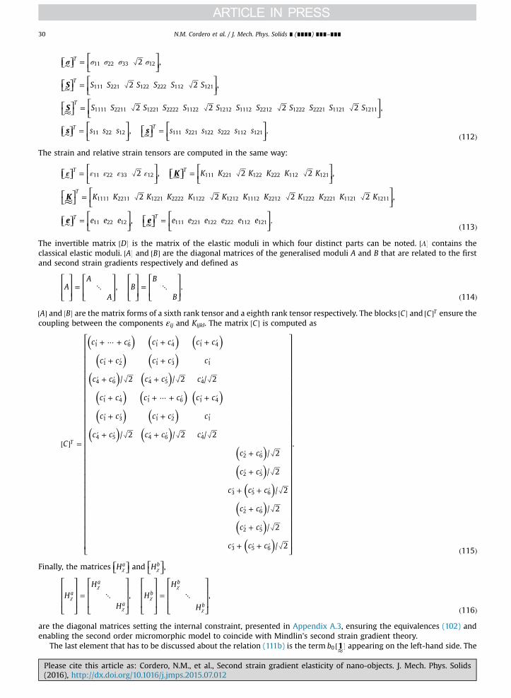
N.M. Cordero et al. / J. Mech. Phys. Solids ∎ (∎∎∎∎) ∎∎∎–∎∎∎30
⎡⎣ ⎤⎦ ⎡⎣⎢
⎤⎦⎥
⎡⎣ ⎤⎦⎡⎣⎢
⎤⎦⎥
⎡⎣ ⎤⎦⎡⎣⎢
⎤⎦⎥
⎡⎣ ⎤⎦ ⎡⎣⎢
⎤⎦⎥
⎡⎣ ⎤⎦⎡⎣⎢
⎤⎦⎥
S
S
s s
S S S S S S
S S S S S S S S S S S S
s s s s s s s s s
2 ,
2 2 ,
2 2 2 2 ,
, .112
T
T
T
T T
11 22 33 12
111 221 122 222 112 121
1111 2211 1221 2222 1122 1212 1112 2212 1222 2221 1121 1211
11 22 12 111 221 122 222 112 121
≈
σ σ σ σ σ=
=
=
= =( )∼ ∼
∼
∼
The strain and relative strain tensors are computed in the same way:
⎡⎣ ⎤⎦ ⎡⎣⎢
⎤⎦⎥ ⎡⎣ ⎤⎦ ⎡
⎣⎢⎤⎦⎥
⎡⎣ ⎤⎦⎡⎣⎢
⎤⎦⎥
⎡⎣ ⎤⎦ ⎡⎣⎢
⎤⎦⎥
⎡⎣ ⎤⎦⎡⎣⎢
⎤⎦⎥
K
K
e e
K K K K K K
K K K K K K K K K K K K
e e e e e e e e e
2 , 2 2 ,
2 2 2 2 ,
, .113
T T
T
T T
11 22 33 12 111 221 122 222 112 121
1111 2211 1221 2222 1122 1212 1112 2212 1222 2221 1121 1211
11 22 12 111 221 122 222 112 121
≈
ε ε ε ε ε= =
=
= =( )
∼
∼ ∼
The invertible matrix D[ ] is the matrix of the elastic moduli in which four distinct parts can be noted. Λ[ ] contains theclassical elastic moduli. A[ ] and B[ ] are the diagonal matrices of the generalised moduli A and B that are related to the firstand second strain gradients respectively and defined as
⎡
⎣⎢⎢
⎤
⎦⎥⎥
⎡
⎣⎢⎢
⎤
⎦⎥⎥
⎡
⎣⎢⎢
⎤
⎦⎥⎥
⎡
⎣⎢⎢
⎤
⎦⎥⎥A
A
AB
B
B, .
114= ⋱ = ⋱
( )
A[ ] and B[ ] are the matrix forms of a sixth rank tensor and a eighth rank tensor respectively. The blocks C[ ] and C T[ ] ensure thecoupling between the components εij and Kijkl. The matrix C[ ] is computed as
⎡
⎣
⎢⎢⎢⎢⎢⎢⎢⎢⎢⎢⎢⎢⎢⎢⎢⎢⎢⎢⎢⎢⎢⎢⎢⎢⎢⎢⎢⎢
⎤
⎦
⎥⎥⎥⎥⎥⎥⎥⎥⎥⎥⎥⎥⎥⎥⎥⎥⎥⎥⎥⎥⎥⎥⎥⎥⎥⎥⎥⎥
C
c c c c c c
c c c c c
c c c c c
c c c c c c
c c c c c
c c c c c
c c
c c
c c c
c c
c c
c c c
/ 2 / 2 / 2
/ 2 / 2 / 2
/ 2
/ 2
/ 2
/ 2
/ 2
/ 2
.
115
T
1 6 1 4 1 4
1 2 1 3 1
4 6 4 5 4
1 4 1 6 1 4
1 3 1 2 1
4 5 4 6 4
2 6
2 5
3 5 6
2 6
2 5
3 5 6
( ) ( ) ( )( ) ( )
( ) ( )( ) ( ) ( )( ) ( )
( ) ( )( )( )
( )( )( )
( )
[ ] =
′ + ⋯ + ′ ′ + ′ ′ + ′
′ + ′ ′ + ′ ′
′ + ′ ′ + ′ ′
′ + ′ ′ + ⋯ + ′ ′ + ′
′ + ′ ′ + ′ ′
′ + ′ ′ + ′ ′
′ + ′
′ + ′
′ + ′ + ′
′ + ′
′ + ′
′ + ′ + ′ ( )
Finally, the matrices ⎡⎣ ⎤⎦Haχ and ⎡⎣ ⎤⎦Hb
χ ,
⎡
⎣
⎢⎢⎢
⎤
⎦
⎥⎥⎥
⎡
⎣
⎢⎢⎢
⎤
⎦
⎥⎥⎥
⎡
⎣
⎢⎢⎢
⎤
⎦
⎥⎥⎥
⎡
⎣
⎢⎢⎢
⎤
⎦
⎥⎥⎥H
H
HH
H
H
, ,
116
a
a
a
b
b
b
= ⋱ = ⋱
( )
χ
χ
χ
χ
χ
χ
are the diagonal matrices setting the internal constraint, presented in Appendix A.3, ensuring the equivalences (102) andenabling the second order micromorphic model to coincide with Mindlin's second strain gradient theory.
The last element that has to be discussed about the relation (111b) is the term b 10 [≈] appearing on the left-hand side. The
Please cite this article as: Cordero, N.M., et al., Second strain gradient elasticity of nano-objects. J. Mech. Phys. Solids(2016), http://dx.doi.org/10.1016/j.jmps.2015.07.012i

N.M. Cordero et al. / J. Mech. Phys. Solids ∎ (∎∎∎∎) ∎∎∎–∎∎∎ 31
initial higher order stress, or cohesion modulus, b0, is present in some components of the triple stress tensor S≈. Thesecomponents are identified in Eq. (99c) as having the form Skkll, Sklkl and Skllk, so that
⎡⎣ ⎤⎦ ⎡⎣⎢
⎤⎦⎥b b b b b b b1 0 0 0 0 0 0 . 117
T T
0 013 0
23 0 0
13 0
23 0≈ = ( )
The principle of virtual work, in the absence of body forces, stipulates that, for all virtual DOF[ ]⁎ ,
⎜ ⎟⎡⎣⎢
⎤⎦⎥
⎛⎝
⎞⎠s e S K s e S K t u t tdV dS: : :: . : .
118V V≈∫ ∫≈σ ε χ χ+ + ⋮ + ⋮ + = + ∼ + ∼ ⋮( ) ∼ ∼ ∼∼ ∼ ∼∼
⁎ ⁎ ⁎ ⁎ ⁎∂
⁎ ⁎ ⁎
which can be translated into the following matrix form:
⎡⎣⎢
⎤⎦⎥
⎡⎣⎢
⎤⎦⎥STRESS STRAIN dV t DOF dS
119VT
VT∫ ∫[ ] = [ ]
( )⁎
∂⁎
⎡⎣⎢
⎤⎦⎥
⎡⎣⎢
⎤⎦⎥
⎡⎣⎢
⎤⎦⎥STRAIN D STRAIN dV t DOF dS
120VT
VT∫ ∫[ ] = [ ]
( )⁎
∂⁎
⎡⎣⎢
⎤⎦⎥
⎡⎣⎢
⎤⎦⎥
⎡⎣⎢
⎤⎦⎥
⎡⎣⎢
⎤⎦⎥DOF D DOF dV t DOF dSB B .
121VT
matrixT
matrixV
T∫ ∫[ ][ ] = [ ]( )
⁎∂
⁎
The matrix form of the problem to solve then takes the usual form
F K DOF , 122[ ] = [ ][ ] ( )
with the generalised stiffness matrix,
⎡⎣⎢
⎤⎦⎥
⎡⎣⎢
⎤⎦⎥
⎡⎣⎢
⎤⎦⎥K D dVB B ,
123Vmatrix
Tmatrix∫ [ ]=
( )
and
⎡⎣⎢
⎤⎦⎥F t dS.
124VT∫= [ ]
( )∂
An incremental form of the algorithm is used so that the unknowns are the increment of DOFs, STRESS D STRAINΔ[ ] = [ ] Δ[ ]and b0 does not arise in Eq. (120).
The 2 in STRESS[ ] and STRAIN[ ] are such that the chosen form of the power density of internal forces given in Eq. (87) isrespected,
⎡⎣ ⎤⎦STRESS STRAIN s e S K s e S K , 125T
ij ij ij ij ijk ijk ijk ijk ijkl ijklσ ε[ ] = + + + + ( )⁎ ⁎ ⁎ ⁎ ⁎ ⁎
this is the reason why several coefficients of the matrices Bmatrix[ ], C[ ] and b 10 [≈] were multiplied by 2 1( )± in order to fit thischosen form and to end up with the same relations as formulated in the second order micromorphic model. For example,the strains given in Eq. (91) remain
u u e K
e K K
, , ,
, , 126
ij i j j i ij ij ij ijk ij k
ijk ijk ijk ijkl ijk l
12 , , ,
,
( )ε ε χ χ
χ χ
= + = − =
= − = ( )
and more particularly, as the modified coefficients are related to εij, eij, Kijk, eijk and Kijkl when i j≠ , we have
⎛⎝⎜
⎞⎠⎟
u uu u2
2 212
,127
121,2 2,1
12 1,2 2,1ε ε= + ≡ = +( )
e K e K2 2 2 2 2 , 128121 12,1 121 121 121 121 121 121χ χ χ χ= − = − ≡ = − ( )
K K2 2 . 1291221 122,1 1221 122,1χ χ= ≡ = ( )
References
Agrawal, R., Peng, B., Gdoutos, E.E., Espinosa, H.D., 2008. Elasticity size effects in ZnO nanowires—a combined experimental–computational approach. NanoLett. 8 (11), 3668–3674.
Altenbach, H., Eremeyev, V.A., 2011. On the shell theory on the nanoscale with surface stresses. Int. J. Eng. Sci. 49, 1294–1301.Altenbach, H., Eremeyev, V.A., Lebedev, L.P., 2011. On the spectrum and stiffness of an elastic body with surface stresses. Z. Angew. Math. Mech. 91, 699–710.
Please cite this article as: Cordero, N.M., et al., Second strain gradient elasticity of nano-objects. J. Mech. Phys. Solids(2016), http://dx.doi.org/10.1016/j.jmps.2015.07.012i

N.M. Cordero et al. / J. Mech. Phys. Solids ∎ (∎∎∎∎) ∎∎∎–∎∎∎32
Altenbach, H., Eremeyev, V.A., Morozov, N.F., 2012. Surface viscoelasticity and effective properties of thin-walled structures at the nanoscale. Int. J. Eng. Sci.59, 83–89.
Amiot, F., 2013. An Euler–Bernoulli second strain gradient beam theory for cantilever sensors. Philos. Mag. Lett. 93, 204–212.Auffray, N., 2014. Analytical expressions for odd-order anisotropic tensor dimension. C. R. Méc. 342, 284–291.Auffray, N., dell'Isola, F., Eremeyev, V., Madeo, A., Rosi, G., 2013a. Analytical continuum mechanics à la Hamilton–Piola: least action principle for second
gradient continua and capillary fluids. Mech. Math. Solids, http://dx.doi.org/10.1177/1081286513497616.Auffray, N., Le Quang, H., He, Q.C., 2013b. Matrix representations for 3d strain-gradient elasticity. J. Mech. Phys. Solids 61, 1202–1223.Besson, J., Cailletaud, G., Chaboche, J.-L., Forest, S., Blétry, M., 2009. Non-Linear Mechanics of Materials. Series: Solid Mechanics and Its Applications, vol. 167.
Springer, 433 pp, ISBN: 978-90-481-3355-0.Boehme, T., Dreyer, W., Mueller, W.H., 2007. Determination of stiffness and higher gradient coefficients by means of the embedded-atom method—an
approach for binary alloys. Contin. Mech. Thermodyn. 18, 411–441.Casal, P., 1961. La capillarité interne. Cah. Groupe Français d'Etudes Rhéol. 6, 31–37.Casal, P., 1963. Capillarité interne en mecanique. C.R. Acad. Sci. Paris 256, 3820–3822.Casal, P., 1972. La théorie du second gradient et la capillarité. C.R. Acad. Sci. Paris 274, 1571–1574.Casal, P., Gouin, H., 1985. Relation entre l’équation de l’énergie et l’équation du mouvement en théorie de Korteweg de la capillarité. C. R. Séances Acad. Sci.
Série 2, Méc. Phys. Chim. Sci. Univers. Sci. Terre 300, 231–234.Chhapadia, P., Mohammadi, P., Sharma, P., 2011. Curvature-dependent surface energy and implications for nanostructures. J. Mech. Phys. Solids 59,
2103–2115.Chhapadia, P., Mohammadi, P., Sharma, P., 2012. Erratum-Curvature-dependent surface energy and implications for nanostructures. J. Mech. Phys. Solids 60,
1241–1242.Cordero, N.M., 2011. A Strain Gradient Approach to the Mechanics of Micro and Nanocrystals (Ph.D. thesis). Mines ParisTech.Craighead, H.G., 2000. Nanoelectromechanical systems. Science 290 (5496), 1532–1535.Danescu, A., 2012. Hyper-pre-stress vs. strain-gradient for surface relaxation in diamond-like structures. J. Mech. Phys. Solids 60, 623–642.Danescu, A., Grenet, G., 2012. Continuum strain-gradient elasticity from discrete valence force field model for diamond-like crystals. Int. J. Fract. 174, 95–102.Davydov, D., Javili, A., Steinmann, P., 2013. On molecular statics and surface-enhanced continuum modeling of nano-structures. Comput. Mater. Sci. 69,
510–519.Dell'Isola, F., Seppecher, P., 1995. The relationship between edge contact forces, double forces and intersticial working allowed by the principle of virtual
power. C.R. Acad. Sci. Paris IIb 321, 303–308.Dell'Isola, F., Seppecher, P., 1997. Edge contact forces and quasi-balanced power. Meccanica 32, 33–52.Dell'Isola, F., Seppecher, P., Madeo, A., 2012. How contact interactions may depend on the shape of Cauchy cuts in N-th gradient continua: approach “à la
D'Alembert”. Z. Angew. Math. Phys. 63, 1119–1141.Dingreville, R., Abdelmalek, H., Berbenni, S., 2014. From coherent to incoherent mismatched interfaces: a generalized continuum formulation of surface
stresses. J. Mech. Phys. Solids 72, 40–60.Dingreville, R., Qu, J., Cherkaoui, M., 2005. Surface free energy and its effect on the elastic behavior of nano-sized particles, wires and films. J. Mech. Phys.
Solids 53 (8), 1827–1854.Dingreville, R., Qu, J.M., 2008. Interfacial excess energy, excess stress and excess strain in elastic solids: planar interfaces. J. Mech. Phys. Solids 56,
1944–1954.Dormieux, L., Kondo, D., 2013. Non linear homogenization approach of strength of nanoporous materials with interface effects. Int. J. Eng. Sci. 71, 102–110.Duan, H.L., Wang, J., Karihaloo, B.L., 2009. Theory of elasticity at the nanoscale. Adv. Appl. Mech. 42, 1–68.Feng, X.L., He, R., Yang, P., Roukes, M.L., 2007. Very high frequency silicon nanowire electromechanical resonators. Nano Lett. 7 (7), 1953–1959.Forest, S., 2009. The micromorphic approach for gradient elasticity, viscoplasticity and damage. ASCE J. Eng. Mech. 135, 117–131.Forest, S., Aifantis, E.C., 2010. Some links between recent gradient thermo-elasto-plasticity theories and the thermomechanics of generalized continua. Int.
J. Solids Struct. 47, 3367–3376.Forest, S., Cordero, N.M., Busso, E.P., 2011. First vs. second gradient of strain theory for capillarity effects in an elastic fluid at small length scales. Comput.
Mater. Sci. 50, 1299–1304.Forest, S., Sievert, R., 2003. Elastoviscoplastic constitutive frameworks for generalized continua. Acta Mech. 160, 71–111.Germain, P., 1973a. La méthode des puissances virtuelles en mécanique des milieux continus. Première partie: Théorie du second gradient. J. Méc. 12,
235–274.Germain, P., 1973b. The method of virtual power in continuum mechanics. Part 2: microstructure. SIAM J. Appl. Math., 556–575.Gu, S.T., Liu, J.T., He, Q.C., 2014. Size-dependent effective elastic moduli of particulate composites with interfacial displacement and traction discontinuities.
Int. J. Solids Struct. 51, 2283–2296.Gurtin, M.E., Murdoch, A.I., 1975. Continuum Theory of Elastic-Material Surfaces. Arch. Ration. Mech. Anal. 57, 291–323.Gurtin, M.E., Murdoch, A.I., 1978. Surface stress in solids. Int. J. Solids Struct. 14, 431–440.He, Q.C., Feng, Z.Q., 2012. Homogenization of layered elastoplastic composites: theoretical results. Int. J. Non-Linear Mech. 47, 367–376.Hervé-Luanco, E., 2014. Elastic behavior of composites containing multi-layer coated particles with imperfect interface bonding conditions and application
to size effects and mismatch in these composites. Int. J. Solids Struct. 51, 2865–2877.Hoang, M.T., Yvonnet, J., Mitrushchenkov, A., Chambaud, G., 2013. First-principles based multiscale model of piezoelectric nanowires with surface effects. J.
Appl. Phys. 113.Javili, A., dell'Isola, F., Steinmann, P., 2013. Geometrically nonlinear higher-gradient elasticity with energetic boundaries. J. Mech. Phys. Solids 61, 2381–2401.Javili, A., Kaessmair, S., Steinmann, P., 2014. General imperfect interfaces. Comput. Methods Appl. Mech. Eng. 275, 76–97.Javili, A., McBride, A., Mergheim, J., Steinmann, P., Schmidt, U., 2013. Micro-to-macro transitions for continua with surface structure at the microscale. Int. J.
Solids Struct. 50, 2561–2572.Javili, A., McBride, A., Steinmann, P., Reddy, B., 2014. A unified computational framework for bulk and surface elasticity theory: a curvilinear-coordinate-
based finite element methodology. Comput. Mech. 54, 745–762.Javili, A., McBride, A., Steinmann, P., Reddy, B.D., 2012. Relationships between the admissible range of surface material parameters and stability of linearly
elastic bodies. Philos. Mag. 92 (28–30), 3540–3563.Javili, A., Steinmann, P., 2010. On thermomechanical solids with boundary structures. Int. J. Solids Struct. 47 (24), 3245–3253.Javili, A., Steinmann, P., 2011. A finite element framework for continua with boundary energies. Part III: the thermomechanical case. Comput. Methods Appl.
Mech. Eng. 200, 1963–1977.Lazar, M., Maugin, G.A., Aifantis, E., 2006a. Dislocations in second strain gradient elasticity. Int. J. Solids Struct. 43, 1787–1817.Lazar, M., Maugin, G.A., Aifantis, E.C., 2006b. On a theory of nonlocal elasticity of bi-Helmholtz type and some applications. Int. J. Solids Struct. 43,
1404–1421.Magoariec, H., Danescu, A., 2009. Modeling macroscopic elasticity of porous silicon. In: Nassiopoulou, A., Sailor, M., Canham, L., Schmuki, P. (Eds.), Physica
Status Solidi C, vol. 6. pp. 1680–1684.Maranganti, R., Sharma, P., 2007. A novel atomistic approach to determine strain-gradient elasticity constants: tabulation and comparison for various
metals, semiconductors, silica, polymers and the (ir) relevance for nanotechnologies. J. Mech. Phys. Solids 55, 1823–1852.Marcadon, V., Brown, D., Hervé, E., Mele, P., Alberola, N.D., Zaoui, A., 2013. Confrontation between Molecular Dynamics and micromechanical approaches to
investigate particle size effects on the mechanical behaviour of polymer nanocomposites. Comput. Mater. Sci. 79, 495–505.Marcadon, V., Hervé, E., Zaoui, A., 2007. Micromechanical modeling of packing and size effects in particulate composites. Int. J. Solids Struct. 44, 8213–8228.
Please cite this article as: Cordero, N.M., et al., Second strain gradient elasticity of nano-objects. J. Mech. Phys. Solids(2016), http://dx.doi.org/10.1016/j.jmps.2015.07.012i

N.M. Cordero et al. / J. Mech. Phys. Solids ∎ (∎∎∎∎) ∎∎∎–∎∎∎ 33
McDowell, M.T., Leach, A.M., Gall, K., 2008. Bending and tensile deformation of metallic nanowires. Model. Simul. Mater. Sci. Eng. 16, 045003.Mindlin, R.D., 1964. Micro-structure in linear elasticity. Arch. Ration. Mech. Anal. 16 (1), 51–78.Mindlin, R.D., 1965. Second gradient of strain and surface-tension in linear elasticity. Int. J. Solids Struct. 1, 417–438.Mindlin, R.D., Eshel, N.N., 1968. On first strain gradient theories in linear elasticity. Int. J. Solids Struct. 4, 109–124.Mitrushchenkov, A., Chambaud, G., Yvonnet, J., He, Q.C., 2010. Towards an elastic model of wurtzite AlN nanowires. Nanotechnology 21.Mohammadi, P., Liu, L.P., Sharma, P., Kukta, R.V., 2013. Surface energy, elasticity and the homogenization of rough surfaces. J. Mech. Phys. Solids 61, 325–340.Müller, P., Saúl, A., 2004. Elastic effects on surface physics. Surf. Sci. Rep. 54 (5–8), 157–258.Ojaghnezhad, F., Shodja, H.M., 2013. A combined first principles and analytical determination of the modulus of cohesion, surface energy, and the additional
constants in the second strain gradient elasticity. Int. J. Solids Struct. 50, 3967–3974.Olive, M., Auffray, N., 2013. Symmetry classes for even-order tensors. Math. Mech. Complex Syst. 1, 177–210.Olive, M., Auffray, N., 2014. Symmetry classes for odd-order tensors. Z. Angew. Math. Mech. 94, 421–447.Polizzotto, C., 2013. A second strain gradient elasticity theory with second velocity gradient inertia—Part I: constitutive equations and quasi-static behavior.
Int. J. Solids Struct. 50, 3749–3765.Ru, C., Aifantis, E., 1993. A simple approach to solve boundary value problems in gradient elasticity. Acta Mech. 101, 59–68.Sadeghian, H., Yang, C.K., Goosen, J.F.L., Van der Drift, E., Bossche, A., French, P.J., Van Keulen, F., 2009. Characterizing size-dependent effective elastic
modulus of silicon nanocantilevers using electrostatic pull-in instability. Appl. Phys. Lett. 94, 221903.Sanii, B., Ashby, P.D., 2010. High sensitivity deflection detection of nanowires. Phys. Rev. Lett. 104 (14), 147203.Shodja, H.M., Ahmadpoor, F., Tehranchi, A., 2012. Calculation of the additional constants for fcc materials in second strain gradient elasticity: behavior of a
nano-size Bernoulli–Euler beam with surface effects. J. Appl. Mech.—Trans. ASME 79, 021008.Shu, J., 1998. Scale-dependent deformation of porous single crystals. Int. J. Plast. 14, 1085–1107.Thomas, O., Ponchet, A., Forest Editors, S., 2011. Mechanics of Nano-objects. Presses des Mines, Paris, 380 pp, ISBN: 978-2911256-67-7.Toupin, R.A., 1962. Elastic materials with couple-stresses. Arch. Ration. Mech. Anal. 11 (1), 385–414.Upadhyay, M.V., Capolungo, L., Taupin, V., Fressengeas, C., 2012. Elastic constitutive laws for incompatible crystalline media: the contributions of dis-
locations, disclinations and G-disclinations. Philos. Mag. 93, 794–832.Villain, P., Beauchamp, P., Badawi, K.F., Goudeau, P., Renault, P., 2004. Atomistic calculation of size effects on elastic coefficients in nanometre-sized tungsten
layers and wires. Scr. Mater. 50, 1247–1251.Yvonnet, J., Le Quang, H., He, Q.C., 2008. An XFEM/level set approach to modelling surface/interface effects and to computing the size-dependent effective
properties of nanocomposites. Comput. Mech. 42, 119–131.Yvonnet, J., Mitrushchenkov, A., Chambaud, G., He, Q.C., 2011. Finite element model of ionic nanowires with size-dependent mechanical properties de-
termined by ab initio calculations. Comput. Methods Appl. Mech. Eng. 200, 614–625.Yvonnet, J., Mitrushchenkov, A., Chambaud, G., He, Q.C., Gu, S.T., 2012. Characterization of surface and nonlinear elasticity in wurtzite ZnO nanowires.
Journal of Applied Physics, 111.Zhang, X., Sharma, P., 2005. Inclusions and inhomogeneities in strain gradient elasticity with couple stresses and related problems. International Journal of
Solids and Structures 42, 3833–3851.
Please cite this article as: Cordero, N.M., et al., Second strain gradient elasticity of nano-objects. J. Mech. Phys. Solids(2016), http://dx.doi.org/10.1016/j.jmps.2015.07.012i


![PLANE STRAIN PROBLEMS IN SECOND-ORDER ELASTICITY THEORY · PDF filePLANE STRAIN PROBLEMS IN SECOND-ORDER ... Green and Shield [4], ... Plane strain problems in second-order elasticity](https://static.fdocuments.in/doc/165x107/5aa819c67f8b9ac5258b68be/plane-strain-problems-in-second-order-elasticity-theory-strain-problems-in-second-order.jpg)


