Physics Letters B 704 (2011) 66–73

Contents lists available at SciVerse ScienceDirect

Physics Letters B

www.elsevier.com/locate/physletb

Second order thermal corrections to electron wavefunction

Mahnaz Q. Haseeb a,∗, Samina S. Masood b

a Department of Physics, COMSATS Institute of Information Technology, Islamabad, Pakistanb Department of Physics, University of Houston Clear Lake, Houston, TX 77058, United States

a r t i c l e i n f o a b s t r a c t

Article history:Received 17 April 2011Received in revised form 15 July 2011Accepted 21 August 2011Available online 25 August 2011Editor: T. Yanagida

Keywords:RenormalizationFinite temperature field theoryElectron self energyTwo-loop QED corrections

Second order perturbative corrections to electron wavefunction are calculated here, for the first time,at generalized temperature. Calculations of electron self energy are important for the renormalizabilityof electron mass and wavefunction in QED through order by order cancellation of singularities up toorder α2. Cancellation of temperature dependent singularities is demonstrated by incorporating theresults of both orders of integration between cold and hot loops. For finite terms, we have rewrittensecond order thermal corrections as well, in a concise form, to calculate wavefunction renormalizationconstant. Our results are in a form that includes intermediate temperatures T ∼ m (where m is electronmass) while limits of high temperature T � m and low temperature T � m are also retrievablefrom them. A comparison with the existing results is included as well. The renormalized mass andwavefunction are used to calculate particle processes in extremely hot systems such as stellar cores andprimordial nucleosynthesis during very early universe. An application to the latter case is also discussed.

© 2011 Elsevier B.V. All rights reserved.

1. Introduction

Finite temperature effects are applicable to extremely high temperature backgrounds, such as those that were present during primordialnucleosynthesis in the early universe and exist in astrophysical environments, etc. These effects are significant enough and should not beignored in comparison with the vacuum contribution. High temperature and density effects in ultra-relativistic plasma are required tobe incorporated in exceptionally hot early universe and hot and dense systems such as those in supernovae and cores of neutron stars.More recently renewed interest in hot and dense QED plasmas has been generated due to possibility of creating ultra-relativistic electron-positron plasmas with high-intensity lasers (≈ 1018 W/cm2) [1–3]. Two opposite laser pulses hitting a thin gold foil can heat up electronsin the foil up to several MeV (∼ 1010 K).

Particles propagating in vacuum can be assumed to be the ones with interactions switched off. When these particles propagate througha medium, several kinds of interaction processes take place. This makes the properties of the system different from that in which allthe particles are assumed to be completely independent of each other, behaving as freely propagating bare particles. When dealing withextremely hot environments in QED, where the particles propagate in statistical background at energies around the thresholds for particle–antiparticle pair production, temperature effects need to be appropriately taken into account. Such effects arise due to continuous electronand photon exchanges between particles during physical interactions that take place in a heat bath containing hot particles and an-tiparticles. The net statistical effects of background electrons and photons enter the theory through the fermion and boson distributionsrespectively.

Thermal background effects are included through radiative corrections [4,5]. Self energies, self masses and wavefunctions of the prop-agating particles acquire temperature corrections in this environment due to exchanges of energy and momentum with real particles.An exact state of all these background particles is unknown since they regularly fluctuate between different configurations and for thisstatistical approach is incorporated. Finite temperature calculations also provide a guideline to estimate density corrections at higher orderloops through chemical potential effects of the background plasma.

Finite temperature propagators in real time formalism comprise of temperature dependent terms added to the particle propagatorsin vacuum theory [6]. In finite temperature electrodynamics, electric fields are further screened due to such interactions. Temperaturesof interest in such a situation are in the range of a few MeV. Big Bang Nucleosynthesis (BBN) theory, together with precise Wilkinson

* Corresponding author.E-mail address: mahnazhaseeb@comsats.edu.pk (M.Q. Haseeb).

0370-2693/$ – see front matter © 2011 Elsevier B.V. All rights reserved.doi:10.1016/j.physletb.2011.08.057

M.Q. Haseeb, S.S. Masood / Physics Letters B 704 (2011) 66–73 67

Microwave Anisotropy Probe (WMAP) data for cosmic baryon density, leads to tight predictions for light elemental abundances after thebig bang. The electron mass shifts determined through self energy corrections have relevance in primordial nucleosynthesis since theylead to modifications to neutron lifetime and hence helium (4He) abundance parameter. Therefore electron self energy loops need to beevaluated with higher order corrections with more accuracy.

In literature, ways to compute finite temperature effects on phase-space, vertex, mass corrections and photon emission or absorption[7–16] are extensively discussed. Finite temperature wave function renormalization has been dealt with several approaches [9–18], specif-ically in the context of weak decay rates during primordial nucleosynthesis. They agree on using finite temperature Dirac spinors to obtaincorresponding effective projection operator. Differences in the spinors presented in Refs. [17] and [18] were also pointed out [19]. How-ever, their results in case of β-decay and related processes agreed with the ones obtained using the approaches that had already existedfor wave function renormalization, except in case of a scalar boson decay into fermion–antifermion pair.

Real time formalism for calculations at finite temperature [20], provides an ease of obtaining the temperature corrections as additiveterms to usual contribution in vacuum. We have used this formulation for calculation of electron self energy as a second order perturbativecorrection in α. From the self energy expression wavefunction renormalization is obtained, for the first time, in a generalized form suchthat intermediate temperatures T ∼ m are also included while the ranges of high temperature T � m and low temperature T � m, areretrieved from them as the limiting cases. We have to rewrite the previously calculated self-mass of electron in a convenient form tobe able to calculate wavefunction renormalization constant at the two loop level. We evaluate the loops with temperature dependentmomenta integrated before temperature independent variables and vice versa, in the relevant order α2 loops in QED, and compare thesewith the calculations of electron self energy done in Refs. [21,22] earlier. These results of loop integrations makes the calculations of loopmomenta much more simpler and easier to handle.

Section 2 is based on the reexamined and simplified calculations of loop correction up-to two orders in α that contribute to electronself energy in this background. The electron mass shift and its relevance to the 4He abundance parameter at the time of primordialnucleosynthesis is presented in Section 4. The wavefunction renormalization constant is calculated in Section 4 from self energy of electronup to the two loop level. Section 5 comprises of summary of the results.

2. Loop corrections to electron self energy

At one loop level, Feynman diagrams are calculated in usual way by substituting the propagators for electron, positron and photonin vacuum by those at finite temperature. Hot terms correspond to a contribution of real background particles on mass-shell that are inthermal equilibrium. In real time formalism, finite temperature terms remain separate at order α since terms depending on temperature(hot) are additive to temperature independent (cold) terms, in the propagators. Therefore, at one loop level the hot and cold loop momentaare integrated separately. However, in finite temperature field theory, covariance is maintained in real time framework at the cost of brokenLorentz invariance. This invariance is then inserted by hand through a choice of four velocity of the heat bath uμ = (1,0,0,0), that affectsenergy integrations in the loops.

Due to interactions with the background, electron and positron masses are known to get enhanced at one-loop and higher loop levels[4–9]. Photons also acquire dynamically generated mass due to plasma screening effect [23,24]. The presence of effective mass impliesthe fact that propagating particles constantly interact with the background. Radiatively generated thermal mass leads to a mass shift inphysical quantities. This mass acts as a kinematical cut-off for physical processes, e.g., while determining production rate of particles inthe heat bath.

Higher order loop corrections are required to study the perturbative behavior at finite temperature. Two loop integrals comprise of acombination of cold and hot momenta which appear due to an overlap of temperature dependent and temperature independent terms inthe particle propagators. Therefore higher loop integrations involve an overlap of finite and divergent terms due to which these becomeanalytically more complicated, even at the two loop level [24]. Integration of thermal integrals is done here before the temperatureindependent integrals and vice versa, in the rest frame of heat bath. One of the reasons for this is that there is a need to get rid of hotdivergences appearing due to the presence of hot loops.

Renormalization in finite temperature field theories becomes somewhat different from that at zero temperature due to additional hotinfrared divergences at finite temperature. These divergences get removed in particle decay processes via bremstrahlung emission andabsorption effects [5,25]. Temperature itself, however, acts as a regularization parameter for hot ultraviolet divergences. The order by ordercancellation of singularities can be observed through an addition of all the diagrams of same order in α. Order α self energy determinedfor all the possible ranges of temperature valid in QED including T ∼ m was presented [25] as:

Σβ(p) = ΣT =0(p) + α

4π2

[(/p − m)I A + /I + (2m − /p) J A + /J B

](1)

where

I A = 8π

∞∫0

dk

knB(k),

I0

E= −2π3T 2

3E2 vln

1 − v

1 + v,

I · p

p2= −2π3T 2

3E2 v3

{ln

1 − v

1 + v+ 2v

},

with v = |p|p0

, (p0 = E),

J A � −8πb(mβ),J 0

B

E� 4π

[T

E2 vln

1 + v

1 − v

{ma(mβ) − T c(mβ)

} − 3b(mβ)

],

JB · p2

� π2 2

[{E2 − 2

m2}

b(mβ) + 4T

{1

ln1 + v + 2

}{ma(mβ) − T c(mβ)

}],

p v E 3 v 1 − v

68 M.Q. Haseeb, S.S. Masood / Physics Letters B 704 (2011) 66–73

Fig. 1. Two loop electron self energy diagrams.

a(mβ) = ln(1 + e−mβ

), b(mβ) =

∞∑n=1

(−1)n Ei(−nmβ), c(mβ) =∞∑

n=1

(−1)n e−nmβ

n2,

and Ei(−x) is an error integral given by

Ei(−x) = −∞∫

x

dt

te−t .

Renormalization of QED was also established at the one loop level for all relevant ranges of temperature and chemical potential [23,25–27].The calculation of electron self energy at finite temperature is done up-to the two loop level since the electron mass shift has relevance

to primordial nucleosynthesis at the time of BBN. Study of this aspect has acquired even more relevance in recent years since the obser-vational probes such as WMAP had been providing data with unprecedented precision [28–31] for light element abundance parameters.Latest observational probes such as Planck and Herschel have now started providing observational data with further definitive accuracy.

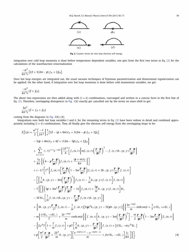
Integrations, at two loop level, over the temperature dependent momenta have been reexamined and wherever needed are re-donefor all the ranges of temperature that are relevant in QED. Two-loop electron self energy diagram with the one-loop vacuum polarizationinsertion as a subdiagram in Fig. 1(a) is omitted here because, as pointed out in Ref. [32] and also checked in Ref. [22], it contributesonly to charge renormalization and has been included here for presenting all combinations expected. The divergences in Fig. 1(a) can beexplicitly removed, however, by adding similar terms from Fig. 2(a).

Electron self energy in Figs. 1(b) and 1(c) is once again rechecked here at the two loop level, from the point of view of renormalization,with integration over hot loop momenta first, in the electron self energy diagrams and vice versa. The overlapping loops in Fig. 1(b) has(non-zero) real terms:

Σb(p) = e4∫

d4k

(2π)4

∫d4l

(2π)4Nb

[{− δ[(p − l)2 − m2]nF (p − l)

l2k2[(p − k)2 − m2][(p − k − l)2 − m2]+ δ(l2)nB(l)

k2[(p − l)2 − m2][(p − k)2 − m2][(p − k − l)2 − m2]}

+ 4π2{

δ(l2)nB(l)δ(k2)nF (k)δ{(p − k − l)2 − m2}nF (p − k − l)

[(p − k)2 − m2][(p − l)2 − m2]+ δ(l2)nB(l)δ{(p − k)2 − m2}nF (p − k)δ{(p − k − l)2 − m2}nF (p − k − l)

k2[(p − l)2 − m2]+ δ(k2)nB(k)δ{(p − l)2 − m2}nF (p − l)δ{(p − k − l)2 − m2}nF (p − k − l)

l2[(p − k)2 − m2]}

+ (l ↔ k) terms

], (2)

with

Nb = [2(

p2 − p · k − p · l + k · l)(/p − /k − /l) − m

{3p2 + k2 + l2 − 2p · k − 2p · l

− 6k · l − 2/p/k + (3/l/k − 2/l/p)} − m2(3/p − 2/k − 2/l) + m3]. (3)

The terms in Eq. (2) have been integrated in detail separately. At two loop level, renormalization of the theory can be proven if hotintegrals are also evaluated before the cold integrals on mass shell and added to the results for loop integrations done in the reverse order.If results from both of these combination of integration orders are not added up, the overlapping ultraviolet divergences do not cancel outexactly. This was not specifically noted in Ref. [22], where a particular order of integrations was not tracked down for the calculations ofthe wavefunction renormalization and therefore, integrations of variables was done arbitrarily. Inclusion of both the orders of integrationsin this manner helps to handle the statistical effects in all possible ways. We demonstrate this, in the following, by writing down resultsfrom overlapping terms containing ultraviolet divergences arising from the terms with only one statistical distribution function each. If

M.Q. Haseeb, S.S. Masood / Physics Letters B 704 (2011) 66–73 69

Fig. 2. Counter terms for two loop electron self energy.

integration over cold loop momenta is done before temperature dependent variables, one gets from the first two terms in Eq. (2) for thecalculations of the wavefunction renormalization

−α2

4π3ε

[2/I + 3(2m − /p) J A + 2/J B

].

Once hot loop energies are integrated out, the usual vacuum techniques of Feynman parametrization and dimensional regularization canbe applied. On the other hand, if integration over hot loop momenta is done before cold momentum variables, we get:

−α2

4π3ε[/I + /J B ].

The above two expressions are then added along with (l ↔ k) combinations, rearranged and written in a concise form in the first line ofEq. (3). Therefore, overlapping divergences in Fig. 1(b) exactly get cancelled out by the terms on mass-shell to get:

3α2

4π3ε[/I + J A + /J B ]

coming from the diagrams in Fig. 2(b)–(d).Integrations over both hot loop variables l and k, for the remaining terms in Eq. (2) have been redone in detail and combined appro-

priately including (l ↔ k) combinations. They all finally give the electron self energy from the overlapping loops to be:

Σbβ(p) = α2

2

[ −1

2π3

{1

ε

[3/I − (/p + 6m)I A + 3(2m − /p) J A + 3/JB

]

− 3(/p + 4m)I A + 4/I + (12m − 5/p) J A + 2/J B

}

+∞∑

n,r,s=1

(−1)r+1e−rβE{

3T 2

4

[f+(n, r)

{mf+(s, r)

(γ · p

|p|2)2

− f−(s, r)h−(p, γ )γ · p

|p|2}

+ I B

8π

{(4 − /p

γ · p

|p|2)

f+(n, r) + (/p + m)IC

8π

}]

+ (−1)s[

T 2{

f+(n, r)

[γ · p

|p|2(

1 − 3mγ · p

|p|2)

f+(s, r) + 3h−(p, γ )γ · p

|p|2 f−(s, r)

]

−[{

1

mh−(p, γ ) − 3m

(γ · p

|p|2)2}

f+(s, r) − 3

mh+(p, γ ) f−(s, r)

]f−(n, r)

}

− T

{[{(5/p + 3m2 γ · p

|p|2)

γ · p

|p|2 − 12

}f+(n, r) + 5/p

mh−(p, γ ) f−(n, r)

]Ei−

− 3E Ei+[

1

mf−(n, r)h+(p, γ ) − γ · p

|p|2 f+(n, r)h−(p, γ )

]}

+{

3h−(p, γ )γ · p

v2f+(n, r) − 1

mf−(n, r)

[3|p|2h+(p, γ ) − 5E/ph−(p, γ )

]}{2e−rmβ

msinh smβ + 1

T(r Ei+ +s Ei−)

}

− m

{(r Ei+ −s Ei−)

T+ 2e−rmβ

mcosh smβ

}{f−(n, r)

[h−(p, γ ) − 3m

(γ · p

|p|2)2]

− m

2

γ · p

|p|2(

1 − 3mγ · p

|p|2)

f+(n, r)

}

−{

2γ 0T

[1 + T

mf+(s, r)

]+ /pT

[2

mh−(p, γ ) − γ · p

|p|2]}

f−(s, r) + [E Ei+ −mγ 0 Ei−

]

+ /p

[m2 γ · p

2+ 2E2

h−(p, γ )

][e−mβ(s+r) − e−mβ(r−s)

+ β(r Ei+ −s Ei−)

]IC

]}], (4)

2 |p| m m 8π

70 M.Q. Haseeb, S.S. Masood / Physics Letters B 704 (2011) 66–73

where

f±(n, r) ={

1

(n + r)± 1

(n − r)

}, f±(s, r) =

{1

(s + r)± 1

(s − r)

}, h±(p, γ ) =

(γ 0 ± γ · p

v|p|)

,

Ei± = Ei[−mβ(r + s)

] ± Ei[−mβ(r − s)

], I B = 8π

∞∑r=1

(−1)r

∞∫0

dk

ke−rβ(p−k)nB(k), IC = 8π

∞∑r=1

(−1)r

∞∫0

dk

ke−rβknB(k).

The non-vanishing real terms from loop within loop correction Σc(p) in Fig. 1(c) are calculated from

Σc(p) = 4e4∫

d4q

(2π)4

∫d4l

(2π)4

[q2(/q + /l) − 2l · q(/q − 2m) − m2(3/q + /l) + 4m3]

×[

δ(l2)nB(l)

k2[(p − l)2 − m2][(p − k)2 − m2][(p − k − l)2 − m2]+ 4π2

{δ(l2)nB(l)δ(k2)δ{(q − l)2 − m2}nF (q − l)δ(q0 − Eq)nF (q)

2E2q(q0 + Eq)(p − q)2

+ δ(l2)nB(l)δ(k2)nF (q − l)δ{(q − l)2 − m2}nF (q)δ′(q0 − Eq)

2E2q(p − q)2

+ nF (q)δ(k2)nF (q − l)δ{(q − l)2 − m2}nB(p − q)δ(p − q)2

2E2ql2

[δ(q0 − Eq)

(q0 + Eq)+ δ′(q0 − Eq)

]}], (5)

with q = p − k. Carrying out all the integrations in Eq. (5) one by one and then combining them, we get

Σcβ(p) = α2

{2T 2

3m2(/p − m) + mT

∞∑n,r,s=1

(−1)s+r[{

β(r + s)Ei[−mβ(r + s)

]

+ e−mβ(s+r)

m

}{1

(n − r)

[2E

m+ γ 0

(1

2− E2

m2

)+ rβ

(m − /p

2

)]+ 1

(n − s)

[h(p, γ ) + m

γ · p

|p|2]}

+ 1

2(n − r)

{2

m− Eγ 0

m2+ rβ

[h(p, γ ) + m

γ · p

|p|2]

Ei[−mβ(r + s)

]}]

− π T

6|p|∞∑

n,r,s=1

(−1)r+1e−nβE[

h(p, γ )

{[1 + (−1)s]e−mβ(r−n−s)

r − n − s

}

− Tγ · p

|p|2e−mβ(r−n)

r − n+

(2 − mγ · p

|p|2){

mβ(r − n)Ei[−mβ(r − n)

]

− e−mβ(r−n) + β[1 + (−1)1+s]Ei

[−mβ(r − n − s)]}]}

. (6)

Fig. 1(c) gives only finite result, as was the case in Ref. [22] as well. The additional hot infrared divergences I A , I B , and IC in Fig. 1(b)that appear at finite temperatures are appropriately removed in particle decay processes via bremstrahlung emission and absorption effects[5,25]. Temperature acts as a regularization parameter for hot ultraviolet divergences. Thus after rearranging the finite terms we obtaintemperature corrections to electron mass and wavefunction. Further, even for finite terms, in Eqs. (4) and (6), the integrations are redonein a manner that not only sufficiently eases the calculations but results are also simpler. This is obvious from the expressions of finiteterms here as compared to those in Ref. [22].

3. The electron mass shift

To incorporate finite temperature effects in physical processes beyond tree level, one needs to have a consistent method of temperaturedependent renormalization. As already mentioned, renormalizability of electron mass was done through the order by order cancellationof singularities up to two loop level even in Ref. [22] and redone here more explicitly. It can be checked that the second order in αcorrection is much smaller than the first order contribution so that the perturbative behavior is valid. The shift in the electron mass dueto finite temperature effects is calculated here after we put together results from all the finite terms in electron self energy up-to secondorder in α using Eqs. (4) and (6). As electrons acquire temperature dependent (or thermal) mass from the medium, following Ref. [5], thephysical mass of electron at one loop was obtained in Ref. [25] in generalized form, by writing

Σ(p) = A(p)Eγ0 − B(p)�p · �γ − C(p),

where A(p), B(p), and C(p) are the relevant coefficients. Taking inverse of the propagator with momentum and mass term separated as

S−1(p) = (1 − A)Eγ 0 − (1 − B)p · γ − (m − C),

M.Q. Haseeb, S.S. Masood / Physics Letters B 704 (2011) 66–73 71

physical mass mphy = m + δm(1) + δm(2) , was deduced by locating pole of the propagator i(/p+m)

p2−m2+iε. δm(1) and δm(2) is the shift in electron

mass due to temperature effects at one and two loop level respectively. Using the same procedure, relative shift in electron mass at thetwo loop level was obtained [22]. On recombining similar summations and rearranging, the shift in electron mass becomes:

δm(2)

m= 2α2

∞∑r=1

[T 2

m2

{r+1∑n=3

(−1)n+r+1 πm

6E v

e−β(rE+mn)

n

− 3

8(−1)r e−rβE

E2 v2

[9E2

2m2+ 6

r+1∑s=3

1

s+ 4

r+1∑n,s=3

1

ns+ (−1)s−r

{9E

m

(3 + 4

r+1∑s=3

1

s

)

+ 2

(E2 v2

m2− 3

)(9 + 18

r+1∑s=3

1

s+ 8

r+1∑n,s=3

1

ns

)}]+ 4

E2 v2

}

− m2

π2c(mβ) − T

m

{π

6E v

r+1∑s=2

s+1∑n=1

e−β(rE+mn)

n

[1 − {

(−1)r+n − (−1)s+n}]

+[{

Ei(−mβ) − Ei(−2mβ)}{9E

4

(E

E2 v2− 1

m

)+

(5E

m− 21 + E2

2m2

) r+1∑n=3

1

n

}

+{

9

4v2−

s+1∑n=1

r+1∑s=3

[1 − E2

(1

2m2+ 3

E2 v2

)+ 3E

m

]}(−1)s Ei(−smβ)

]

+ e−rmβ

{[9E

2v2+ 2

(3E

v2+ 3E2 v2

m− 5E

) r+1∑n=3

1

n

] ∞∑s=1

sinh smβ − 3m3

E2 v2

(3

4−

r+1∑n=3

1

n

) ∞∑s=1

cosh smβ

}}

+{

9m

4E2 v2

(E3 + m3

2

)+

[3m

E2 v2

(E3 + m3) + 5mE − 3E2 v2

] r+1∑n=3

1

n

}{Ei(−mβ) − 2 Ei(−2mβ)

}

−r+1∑n=3

{r+1∑s=1

(−1)s

n

[m2r

2e−smβ +

{sE

(2m − E2

m

)+ m2(s − r)

2

}Ei(−smβ)

]

− πm2

3E v

[e−βrE(−1)n+r(n + 1) −

r+1∑s=2

(−1)n+s

]Ei(−nmβ)

}]. (7)

These self energy and self mass corrections to electrons are of significance for primordial abundances of light elements. During pri-mordial nucleosynthesis era, when temperature was suitable enough to synthesize nuclei of light elements (T ∼ 0.1–10 MeV), nucleoncapturing led to certain bounds on light elemental nuclei abundances, specifically 4He abundance parameter Y which is expected to be0.25 for correspondence with BBN while the measured value, from all the possibilities combined, is slightly less (around 0.24). Theseresults for δm

m are applied to determine the corrections in 4He abundance [10–13,33] as related to the relative mass shift through

Y = 0.2τ

τ= −0.2

λ

λ= 0.04

(m

T

)2δm

m(8)

where ττ is relative change in neutron half life and λ

λis relative change in neutron decay rate.

For one loop corrections estimated in Ref. [33] Y = 0.4×10−3 at T ∼ m and falls to 0.3×10−3 at T ∼ m/3. For example, with energiesaround 1 MeV, Y = 0.31 × 10−4 from one particle irreducible diagram, considered in detail in [34], is just one order of magnitude lesser(∼10)% compared to the one loop contribution. This can be compared with other data which shows that if BBN is correct, Monte Carlosimulations give Y p = 0.2476 ± 0.0004 [35] and through CMB predictions Y p = 0.24819+0.00029

−0.00040 ± 0.0006 (syst.) [36]. It must be noted thatat order α2 temperature correction though small is, however, not negligible to modify Y .

4. Wavefunction renormalization

With finite temperature background in the real-time formalism, since Lorentz invariance is broken, momentum independent renormal-ization constant in vacuum is no longer sufficient. Donoghue and Holstein used temperature dependent propagators to modify electronmass as well as the spinors accordingly [5]. Wave function renormalization for the generalized temperatures does not exist in literature,for two loop corrections. Using the reviewed expression for the electron self energy obtained in Eqs. (4) and (6) relation for wave functionrenormalization constant is derived by taking Z−1 = ∂Σ . This comes out to be

2 ∂/p

72 M.Q. Haseeb, S.S. Masood / Physics Letters B 704 (2011) 66–73

Z−12 = 1 − α

[1

4π

(3

ε− 4

)+ 5

πb(mβ) + I A

4π2− T 2

π v E2ln

1 + v

1 − v

{π2

6− c(mβ) + mβa(mβ)

}]

− α2

[1

4π3

{3

ε(I A + J A) + (3I A + 5 J A)

}− 2T 2

3π3m2+ m

8π

∞∑n,r,s=1

(−1)s+r{

r

[e−mβ(s+r)

m− β(r + s)Ei

{−mβ(r + s)}]}

+ 1

8

∞∑n,r,s=1

(−1)r T

{e−rβE

[f+(s, r)

γ · p

E2 v2+ h(p, γ )

{f−(n, r)

IC

8π− f−(s, r)

}+ f+(n, r)

γ · p

E2 v2

I B

8π− I B IC

64π2

]

+[{

5γ · p

E2 v2f+(n, r) − 5

mh(p, γ ) f−(n, r)

}Ei− + 5E

m2h(p, γ ) f−(n, r)

{2e−rmβ

msinh smβ + β(r Ei+ +s Ei−)

}

+{

2

mh(p, γ ) − γ · p

E2 v2

}f−(s, r)

]}+

{m2

2

γ · p

E2 v2+ 2E2

mh(p, γ )

}{2e−rmβ

msinh smβ + β(r Ei+ −s Ei−)

}IC

8π

]. (9)

From this expression for Z−12 , not only the behavior at intermediate temperatures T ∼ m can be extracted but ranges of high tempera-

ture T � m, low temperature T � m, can be also retrieved from it, as limiting cases.

5. Results and summary

We have demonstrated explicitly the cancellation of overlapping hot and cold divergences in Fig. 1(b) with the counter terms fromFigs. 2(b)–2(d). For this, the results from an integration of hot loops before the cold ones were combined with those from the reverse orderof integration. This has been explicitly checked for the first time, leading to a conclusion that addition of both the possible combinationsof hot and cold loop momenta integrations are a must so that all the statistical effects are appropriately incorporated.

Rewriting electron self energy expressions in QED at the two loop level that were presented in Ref. [22], one obtains a modifiedexpression for relative change in electron mass at the two loop level in Eq. (4). Previously calculated self-mass correction terms areredone for simplicity and conciseness, wherever required, for all the possible ranges of temperature. From these corrections one can thenretrieve results for the temperature ranges of interest here, classified as, high temperature T � m (having mβ → 0 with e−mβ falling off

exponentially as compared to T 2

m2 ), low temperature T � m (with fermions contribution negligible) and intermediate temperatures T ∼ m(by taking mβ → 1).

Self energy and self mass corrections to electron are of significance for primordial abundances since they get dynamically generatedmass due to plasma screening effect. During the era of primordial nucleosynthesis, when temperature was suitable enough to synthesizenuclei of light elements, it led to bounds on 4He abundance. Order α2 temperature correction are not negligible and can serve as one ofthe sources of input for modification in Y .

We calculated here, for the first time, using thermal contributions in the generalized form of temperature, wavefunction renormalizationconstant up to second order in α. Fermions do not pick any contribution from the heat bath at low temperature. Therefore, the secondorder in α corrections to electron self energy at low temperature can be retrieved as a limiting case that contains contribution from hotphotons only. Thus wave function renormalization constant up-to two loops in Eq. (6) in the limit T � m reduces to

Z−12

T �m−−−→ 1 + α

4π

(4 − 3

ε

)− α

4π2

(I A − I0

E

)− α2

4π2

(3 + 1

ε

)I A + 2α2T 2

3π2m2, (10)

which is the same as that in Ref. [37]. The high temperature limit for wave function renormalization constant gives:

Z−12

T �m−−−→ 1 − α

[2I A

π+ 1

4π

(3

ε− 4

)+ 4π T 2

3

]− α2

[1

4π3

{3

ε(I A + J A) + (3I A + 5 J A) − 8T 2

3m2

}

+ 1

8

∞∑n,r,s=1

(−1)r T

{e−rβE

[f+(s, r)

γ · p

E2 v2− I B IC

64π2+ h(p, γ )

{f−(n, r)

IC

8π− f−(s, r)

}+ f+(n, r)

γ · p

E2 v2

I B

8π

+{

2

mh(p, γ ) − γ · p

E2 v2

}f−(s, r)

]}]. (11)

Eq. (8) shows that the leading contribution in this range of temperature, T � m, at the two loop level is 2T 2

3m2 . It is worth mentioningthat thermal corrections, at second order in α, to wavefunction renormalization constant at extreme temperatures (T � m and T � m)are still proportional to T 2

m2 as in case of the self mass of electron. The self-energy expression for intermediate temperatures is somewhatdifferent from the one obtained earlier [22]. Calculations around T ∼ m for mass and wavefunction renormalization constants though stillcumbersome at the two-loop level, are much simpler than those in Ref. [22].

Two loop fermion self energy in QED has been calculated in detail recently [38] using the hard thermal loop (HTL) resummationintroduced by Braaten and Pisarski [39–41]. As far as the renormalization is concerned, HTL do not affect it [38]. Hence Z2 does not getany contribution from HTL here.

Renormalizability of the theory at finite temperature is explicitly established up to order α2 and holds through order by order can-cellation of singularities. This provides a platform to include general effects due to chemical potential in hot and dense background lateron. With an experience of including chemical potential at one loop level, in real time formulation [23,26,27], it is foreseen that two loop

M.Q. Haseeb, S.S. Masood / Physics Letters B 704 (2011) 66–73 73

self energy calculations will be much more complicated but are still worth-doing to develop a calculational technique for high densityhot plasmas, even in case of superfluids inside the cores of neutron stars [42]. The modified wavefunction is expected to affect finitetemperature contributions to electroweak processes [43] as well as neutrino magnetic moments [44] up to the two loop level.

Acknowledgements

One of the authors (M.Q.H.) thanks Higher Education Commission, Pakistan, for providing partial funding under a research grant 20-1925 during this work.

References

[1] E.P. Liang, S.C. Wilks, M. Tabak, Phys. Rev. Lett. 81 (1998) 4887.[2] B. Shen, J. Meyer-ter-Vehn, Phys. Rev. E 65 (2001) 016405.[3] M.H. Thoma, Eur. Phys. J. D 55 (2009) 271;

M.H. Thoma, Rev. Mod. Phys. 81 (2009) 959.[4] H.A. Weldon, Phys. Rev. D 26 (1982) 1394.[5] J.F. Donoghue, B.R. Holstein, Phys. Rev. D 28 (1983) 340;

J.F. Donoghue, B.R. Holstein, Phys. Rev. D 29 (1983) 3004 (Erratum).[6] P. Landsman, Ch.G. Weert, Phys. Rep. 145 (1987) 141.[7] D.A. Dicus, E.W. Kolb, A.M. Gleeson, E.C.G. Sudarshan, V.L. Teplitz, M.S. Turner, Phys. Rev. D 26 (1982) 2694.[8] J.-L. Cambier, J.R. Primack, M. Sher, Nucl. Phys. B 209 (1982) 372.[9] J.F. Donoghue, B.R. Holstein, R.W. Robinett, Ann. Phys. (N.Y.) 164 (1985) 233.

[10] A.E. Johansson, G. Peresutti, B.S. Skagerstam, Nucl. Phys. B 278 (1986) 324.[11] W. Keil, Phys. Rev. D 40 (1989) 1176.[12] R. Baier, E. Pilon, B. Pire, D. Schiff, Nucl. Phys. B 336 (1990) 157.[13] W. Keil, R. Kobes, Physica A 158 (1989) 47.[14] M. LeBellac, D. Poizat, Z. Phys. C 47 (1990) 125.[15] T. Altherr, P. Aurenche, Phys. Rev. D 40 (1989) 4171.[16] R.L. Kobes, G.W. Semeneff, Nucl. Phys. B 260 (1985) 714;

R.L. Kobes, G.W. Semeneff, Nucl. Phys. B 272 (1986) 329.[17] R.F. Sawyer, Phys. Rev. D 53 (1996) 4232.[18] I.A. Chapman, Phys. Rev. D 55 (1997) 6287.[19] S. Esposito, G. Mangano, G. Miele, O. Pisanti, Phys. Rev. D 58 (1998) 105023.[20] V.V. Klimov, Sov. J. Nucl. Phys. 33 (1981) 934;

L. Dolan, R. Jackiw, Phys. Rev. D 9 (1974) 3320;S. Weinberg, Phys. Rev. D 9 (1974) 3357;C. Bernard, Phys. Rev. D 9 (1974) 3312.

[21] Mahnaz Qader Haseeb, Samina S. Masood, K. Ahmed, Phys. Rev. D 44 (1991) 3322.[22] Mahnaz Qader Haseeb, Samina S. Masood, K. Ahmed, Phys. Rev. D 46 (1992) 5633.[23] K. Ahmed, Samina S. Masood, Ann. Phys. (N.Y.) 207 (1991) 460.[24] Samina S. Masood, Mahnaz Q. Haseeb, Int. J. Mod. Phys. A 23 (2008) 4709.[25] K. Ahmed, Samina Saleem Masood, Phys. Rev. D 35 (1987) 1861.[26] K. Ahmed, Samina Saleem Masood, Phys. Rev. D 35 (1987) 4020.[27] Samina S. Masood, Phys. Rev. D 44 (1991) 3943;

Samina S. Masood, Phys. Rev. D 47 (1993) 648.[28] G. Hinshaw, et al., Astrophys. J. Suppl. 180 (2009) 225.[29] C.L. Bennett, et al., Astrophys. J. Suppl. 192 (2011) 17.[30] G. Steigman, Primordial nucleosynthesis after WMAP, chemical abundances in the universe: Connecting first stars to planets, in: K. Cunha, M. Spite, B. Barbuy (Eds.),

Proc. IAU Sympos., vol. 265, 2009, pp. 119–138.[31] G. Steigman, Int. J. Mod. Phys. E. 15 (2005) 1;

G. Steigman, Annu. Rev. Nucl. Part. Sci. 57 (2007) 463.[32] D.A. Dicus, D. Down, E.W. Kolb, Nucl. Phys. B 223 (1983) 525.[33] S. Saleem, Phys. Rev. D 36 (1987) 2602.[34] Mahnaz Q. Haseeb, Omair Sarfaraz, Primordial nucleosynthesis and finite temperature QED, Journal of Cosmology and Astrophysics, May 15, 2011, submitted for publi-

cation.[35] A. Coc, E. Vangioni, J. Phys.: Conf. Ser. 202 (2010) 012001.[36] D.N. Spergel, et al., Astrophys. J. Suppl. 170 (2007) 377.[37] Mahnaz Q. Haseeb, Samina S. Masood, Chin. Phys. C 35 (2011) 608.[38] E. Mottola, Z. Szép, Phys. Rev. D 81 (2010) 025014.[39] E. Braaten, R.D. Pisarski, Nucl. Phys. B 337 (1990) 569.[40] E. Braaten, R.D. Pisarski, Phys. Rev. D 42 (1990) 2156.[41] R.D. Pisarski, Phys. Rev. Lett. 63 (1989) 1129.[42] D. Page, et al., Phys. Rev. Lett. 106 (2011) 081101.[43] Mahnaz Qader Haseeb, Samina S. Masood, Phys. Rev. D 46 (1992) 5110.[44] Samina S. Masood, Phys. Rev. D 48 (1993) 3250.