Second-Order Reliability Formulations in DAKOTA/UQ · Sequential and unilevel methods seek to...

Second-Order Reliability Formulations in DAKOTA/UQ

M. S. Eldred∗

Sandia National Laboratories†, Albuquerque, NM 87185

B.J. Bichon‡

Vanderbilt University, Nashville, TN 37235

Reliability methods are probabilistic algorithms for quantifying the effect of uncertainties in simula-tion input on response metrics of interest. In particular, they compute approximate response functiondistribution statistics (probability, reliability, and response levels) based on specified probability distri-butions for input random variables. In this paper, second-order approaches are explored for both theforward reliability analysis of computing probabilities for specified response levels (the reliability indexapproach (RIA)) and the inverse reliability analysis of computing response levels for specified proba-bilities (the performance measure approach (PMA)). These new methods employ second-order Taylorseries limit state approximations and second-order probability integrations using analytic, numerical,or quasi-Newton limit state Hessians, and are compared with the traditional second-order reliabilitymethod (SORM) as well as two-point limit state approximation methods. These reliability analysismethods are then employed within reliability-based design optimization (RBDO) studies using bi-leveland surrogate-based formulations. These RBDO formulations employ analytic sensitivities of response,reliability, and second-order probability levels with respect to design variables that either augment ordefine distribution parameters for the uncertain variables. Relative performance of these reliabilityanalysis and design algorithms are presented for a number of computational experiments performed us-ing the DAKOTA/UQ software. Results indicate that second-order methods can be both more accuratethrough improved probability estimates and more efficient through accelerated convergence rates.

I. Introduction

Reliability methods are probabilistic algorithms for quantifying the effect of uncertainties in simulation input onresponse metrics of interest. In particular, they perform uncertainty quantification (UQ) by computing approximateresponse function distribution statistics based on specified probability distributions for input random variables. Theseresponse statistics include response mean, response standard deviation, and cumulative or complementary cumulativedistribution function (CDF/CCDF) response level and probability/reliability level pairings. These methods are often moreefficient at computing statistics in the tails of the response distributions (events with low probability) than sampling-basedapproaches since the number of samples required to resolve a low probability can be prohibitive. Thus, these methods,as their name implies, are often used in a reliability context for assessing the probability of failure of a system whenconfronted with an uncertain environment.

A number of classical reliability analysis methods are discussed in Ref. 15, including Mean-Value First-Order Second-Moment (MVFOSM), First-Order Reliability Method (FORM), and Second-Order Reliability Method (SORM). Morerecent methods which seek to improve the efficiency of FORM analysis through limit state approximations include theuse of local and multipoint approximations in Advanced Mean Value methods (AMV/AMV+31) and Two-point AdaptiveNonlinearity Approximation-based methods (TANA28,34), respectively. Each of the FORM-based methods can be em-ployed for “forward” or “inverse” reliability analysis through the reliability index approach (RIA) or performance measureapproach (PMA), respectively, as described in Ref. 27.

The capability to assess reliability is broadly useful within a design optimization context, and reliability-based designoptimization (RBDO) methods are popular approaches for designing systems while accounting for uncertainty. RBDOapproaches may be broadly characterized as bi-level (in which the reliability analysis is nested within the optimization,e.g. Ref. 3), sequential (in which iteration occurs between optimization and reliability analysis, e.g. Refs. 8,33), or unilevel(in which the design and reliability searches are combined into a single optimization, e.g. Ref. 2). Bi-level RBDO methodsare simple and general-purpose, but can be computationally demanding. Sequential and unilevel methods seek to reducecomputational expense by breaking the nested relationship through the use of iterated or simultaneous approaches.

∗Principal Member of Technical Staff, Optimization and Uncertainty Estimation Department, Associate Fellow AIAA.†Sandia is a multiprogram laboratory operated by Sandia Corporation, a Lockheed-Martin Company, for the United States Department of

Energy under Contract DE-AC04-94AL85000.‡NSF IGERT Fellow, Department of Civil and Environmental Engineering.

1 of 23

American Institute of Aeronautics and Astronautics

47th AIAA/ASME/ASCE/AHS/ASC Structures, Structural Dynamics, and Materials Confere1 - 4 May 2006, Newport, Rhode Island

AIAA 2006-1828

This material is declared a work of the U.S. Government and is not subject to copyright protection in the United States.

In order to provide access to a variety of uncertainty quantification capabilities for analysis of large-scale engineeringapplications on high-performance parallel computers, the DAKOTA project10 at Sandia National Laboratories has de-veloped a suite of algorithmic capabilities known as DAKOTA/UQ.29 This package contains the reliability analysis andRBDO capabilities described in this paper, and is freely available for download worldwide through an open source license.

This paper explores a variety of algorithms for performing reliability analysis. In particular, forward and inverse reli-ability analyses are performed using multiple limit state approximation, probability integration, Hessian approximation,and optimization algorithm selections. These uncertainty quantification capabilities are then used as a foundation for ex-ploring RBDO formulations. Sections II and III describe these algorithmic components, Section IV provides computationalresults for four benchmark test problems, and Section V provides concluding remarks.

II. Reliability Method Formulations

A. Mean Value

The Mean Value method (MV, also known as MVFOSM in Ref. 15) is the simplest, least-expensive reliability method be-cause it estimates the response means, response standard deviations, and all CDF/CCDF response-probability-reliabilitylevels from a single evaluation of response functions and their gradients at the uncertain variable means. This approxima-tion can have acceptable accuracy when the response functions are nearly linear and their distributions are approximatelyGaussian, but can have poor accuracy in other situations.

With the introduction of second-order limit state information, a second-order mean can be calculated. This is com-monly combined with a first-order variance, since second-order variance involves higher order distribution moments (skew-ness, kurtosis) which are often unavailable. The expressions for approximate response mean µg, approximate responsestandard deviation σg, response target to approximate probability/reliability level mapping (z̄ → p, β), and probabil-ity/reliability target to approximate response level mapping (p̄, β̄ → z) are

µg = g(µx) +1

2

∑

i

∑

j

Cov(i, j)d2g

dxidxj

(µx) (1)

σg =∑

i

∑

j

Cov(i, j)dg

dxi

(µx)dg

dxj

(µx) (2)

βcdf =µg − z̄

σg

(3)

βccdf =z̄ − µg

σg

(4)

z = µg − σgβ̄cdf (5)

z = µg + σgβ̄ccdf (6)

respectively, where x are the uncertain values in the space of the original uncertain variables (“x-space”) and g(x) is thelimit state function (the response function for which probability-response level pairs are needed). The CDF reliabilityindex βcdf , CCDF reliability index βccdf , first-order CDF probability p(g ≤ z), and first-order CCDF probability p(g > z)are related to one another through

p(g ≤ z) = Φ(−βcdf ) (7)

p(g > z) = Φ(−βccdf ) (8)

βcdf = −Φ−1(p(g ≤ z)) (9)

βccdf = −Φ−1(p(g > z)) (10)

βcdf = −βccdf (11)

p(g ≤ z) = 1 − p(g > z) (12)

where Φ() is the standard normal cumulative distribution function. A common convention in the literature is to define gin such a way that the CDF probability for a response level z of zero (i.e., p(g ≤ 0)) is the response metric of interest.The formulations in this paper are not restricted to this convention and are designed to support CDF or CCDF mappingsfor general response, probability, and reliability level sequences.

2 of 23


B. MPP Search Methods

All other reliability methods solve a nonlinear optimization problem to compute a most probable point (MPP) and thenintegrate about this point to compute probabilities. The MPP search is performed in uncorrelated standard normal space(“u-space”) since it simplifies the probability integration: the distance of the MPP from the origin has the meaningof the number of input standard deviations separating the mean response from a particular response threshold. Thetransformation from correlated non-normal distributions (x-space) to uncorrelated standard normal distributions (u-space)is denoted as u = T (x) with the reverse transformation denoted as x = T−1(u). These transformations are nonlinearin general, and possible approaches include the Rosenblatt,25 Nataf,7 and Box-Cox4 transformations. The nonlineartransformations may also be linearized, and common approaches for this include the Rackwitz-Fiessler23 two-parameterequivalent normal and the Chen-Lind6 and Wu-Wirsching30 three-parameter equivalent normals. The results in this paperemploy the Nataf nonlinear transformation which occurs in the following two steps. To transform between the originalcorrelated x-space variables and correlated standard normals (“z-space”), the CDF matching condition is used:

Φ(zi) = F (xi) (13)

where F () is the cumulative distribution function of the original probability distribution. Then, to transform betweencorrelated z-space variables and uncorrelated u-space variables, the Cholesky factor L of a modified correlation matrix isused:

z = Lu (14)

where the original correlation matrix for non-normals in x-space has been modified for z-space.7

The forward reliability analysis algorithm of computing CDF/CCDF probability/reliability levels for specified responselevels is called the reliability index approach (RIA), and the inverse reliability analysis algorithm of computing responselevels for specified CDF/CCDF probability/reliability levels is called the performance measure approach (PMA).27 Thedifferences between the RIA and PMA formulations appear in the objective function and equality constraint formulationsused in the MPP searches. For RIA, the MPP search for achieving the specified response level z̄ is formulated as

minimize uT u

subject to G(u) = z̄ (15)

and for PMA, the MPP search for achieving the specified reliability/probability level β̄, p̄ is formulated as

minimize ±G(u)

subject to uT u = β̄2 (16)

where u is a vector centered at the origin in u-space and g(x) ≡ G(u) by definition. In the RIA case, the optimal MPPsolution u∗ defines the reliability index from β = ±‖u∗‖2, which in turn defines the CDF/CCDF probabilities (usingEqs. 7-8 in the case of first-order integration). The sign of β is defined by

G(u∗) > G(0) : βcdf < 0, βccdf > 0 (17)

G(u∗) < G(0) : βcdf > 0, βccdf < 0 (18)

where G(0) is the median limit state response computed at the origin in u-space (where βcdf = βccdf = 0 and first-orderp(g ≤ z) = p(g > z) = 0.5). In the PMA case, the sign applied to G(u) (equivalent to minimizing or maximizing G(u))is similarly defined by β̄

β̄cdf < 0, β̄ccdf > 0 : maximize G(u) (19)

β̄cdf > 0, β̄ccdf < 0 : minimize G(u) (20)

and the limit state at the MPP (G(u∗)) defines the desired response level result.When performing PMA with specified p̄, one must compute β̄ to include in Eq. 16. While this is a straightforward one-

time calculation for first-order integrations (Eqs. 9-10), the use of second-order integrations complicates matters since theβ̄ corresponding to the prescribed p̄ is a function of the Hessian of G (see Eq. 33), which in turn is a function of location inu-space. A generalized reliability index (Eq. 48), which would allow a one-time calculation, may not be used since equalitywith uT u is not meaningful. The β̄ target must therefore be updated in Eq. 16 as the minimization progresses (e.g., usingNewton’s method to solve Eq. 33 for β̄ given p̄ and κi). This works best when β̄ can be fixed during the course of anapproximate optimization, such as for the AMV2+ and TANA methods described in Section II.B.1. For PMA withoutlimit state approximation cycles (i.e., PMA SORM), the constraint must be continually updated and the constraintderivative should include ∇uβ̄, which would require third-order information for the limit state to compute derivatives ofthe principal curvatures. This is impractical, so the PMA SORM constraint derivatives are only approximated analyticallyor estimated numerically. Potentially for this reason, PMA SORM has not been widely explored in the literature.

3 of 23


1. Limit state approximations

There are a variety of algorithmic variations that can be explored within RIA/PMA reliability analysis. First, one mayselect among several different limit state approximations that can be used to reduce computational expense during theMPP searches. Local, multipoint, and global approximations of the limit state are possible. Ref. 11 focused on localfirst-order limit state approximations. This paper will focus on local second-order and multipoint approximations:

1. a single second-order Taylor series per response/reliability/probability level in x-space centered at the uncertainvariable means (named AMV2 due to its extension of the Advanced Mean Value (AMV) method).

g(x) ∼= g(µx) + ∇xg(µx)T (x − µx) +1

2(x − µx)T∇2

xg(µx)(x − µx) (21)

2. same as AMV2, except that the Taylor series is expanded in u-space. This option has been termed the u-spaceAMV2 method (note: µu = T (µx) and is nonzero in general).

G(u) ∼= G(µu) + ∇uG(µu)T (u − µu) +1

2(u − µu)T∇2

uG(µu)(u − µu) (22)

3. an initial second-order Taylor series approximation in x-space at the uncertain variable means, with iterative ex-pansion updates at each MPP estimate (x∗) until the MPP converges (named AMV2+ due to its extension of theAMV+ method).

g(x) ∼= g(x∗) + ∇xg(x∗)T (x − x∗) +

1

2(x − x∗)T∇2

xg(x∗)(x − x∗) (23)

4. same as AMV2+, except that the expansions are performed in u-space. This option has been termed the u-spaceAMV2+ method.

G(u) ∼= G(u∗) + ∇uG(u∗)T (u − u∗) +1

2(u − u∗)T∇2

uG(u∗)(u − u∗) (24)

5. a multipoint approximation in x-space. This approach involves a Taylor series approximation in intermediatevariables where the powers used for the intermediate variables are selected to match information at the current andprevious expansion points. Based on the two-point exponential approximation concept (TPEA12), the two-pointadaptive nonlinearity approximation (TANA-334) approximates the limit state as:

g(x) ∼= g(x2) +

n∑

i=1

∂g

∂xi

(x2)x1−pi

i,2

pi

(xpi

i − xpi

i,2) +1

2ε(x)

n∑

i=1

(xpi

i − xpi

i,2)2 (25)

where n is the number of uncertain variables and:

pi = 1 + ln

[

∂g∂xi

(x1)∂g∂xi

(x2)

]

/

ln

[

xi,1

xi,2

]

(26)

ε(x) =H

∑ni=1(x

pi

i − xpi

i,1)2 +∑n

i=1(xpi

i − xpi

i,2)2

(27)

H = 2

[

g(x1) − g(x2) −

n∑

i=1

∂g

∂xi

(x2)x1−pi

i,2

pi

(xpi

i,1 − xpi

i,2)

]

(28)

and x2 and x1 are the current and previous MPP estimates in x-space, respectively. Prior to the availability of twoMPP estimates, x-space AMV+ is used.

6. a multipoint approximation in u-space. The u-space TANA-3 approximates the limit state as:

G(u) ∼= G(u2) +

n∑

i=1

∂G

∂ui

(u2)u1−pi

i,2

pi

(upi

i − upi

i,2) +1

2ε(u)

n∑

i=1

(upi

i − upi

i,2)2 (29)

where:

pi = 1 + ln

[

∂G∂ui

(u1)∂G∂ui

(u2)

]

/

ln

[

ui,1

ui,2

]

(30)

4 of 23


ε(u) =H

∑ni=1(u

pi

i − upi

i,1)2 +∑n

i=1(upi

i − upi

i,2)2

(31)

H = 2

[

G(u1) −G(u2) −

n∑

i=1

∂G

∂ui

(u2)u1−pi

i,2

pi

(upi

i,1 − upi

i,2)

]

(32)

and u2 and u1 are the current and previous MPP estimates in u-space, respectively. Prior to the availability of twoMPP estimates, u-space AMV+ is used.

7. the MPP search on the original response functions without the use of any approximations.

The Hessian matrices in AMV2 and AMV2+ may be available analytically, estimated numerically, or approximatedthrough quasi-Newton updates. The quasi-Newton variant of AMV2+ is conceptually similar to TANA in that bothapproximate curvature based on a sequence of gradient evaluations. TANA estimates curvature by matching values andgradients at two points and includes it through the use of exponential intermediate variables and a single-valued diagonalHessian approximation. Quasi-Newton AMV2+ accumulates curvature over a sequence of points and then uses it directlyin a second-order series expansion. Therefore, these methods may be expected to exhibit similar performance.

The selection between x-space or u-space for performing approximations depends on where the approximation will bemore accurate, since this will result in more accurate MPP estimates (AMV2) or faster convergence (AMV2+, TANA).Since this relative accuracy depends on the forms of the limit state g(x) and the transformation T (x) and is thereforeapplication dependent in general, DAKOTA/UQ supports both options. A concern with approximation-based iterativesearch methods (i.e., AMV2+ and TANA) is the robustness of their convergence to the MPP. It is possible for theMPP iterates to oscillate or even diverge. However, to date, this occurrence has been relatively rare, and DAKOTA/UQcontains checks that monitor for this behavior. Another concern with TANA is numerical safeguarding. First, there is thepossibility of raising negative xi or ui values to nonintegral pi exponents in Eqs. 25, 27-29, and 31-32. This is particularlylikely for u-space. Safeguarding techniques include the use of linear bounds scaling for each xi or ui, offseting negative xi

or ui, or promotion of pi to integral values for negative xi or ui. In numerical experimentation, the offset approach hasbeen the most effective in retaining the desired data matches without overly inflating the pi exponents. Second, thereare a number of potential numerical difficulties with the logarithm ratios in Eqs. 26 and 30. In this case, a safeguardingstrategy is to revert to either the linear (pi = 1) or reciprocal (pi = −1) approximation based on which approximationhas lower error in ∂g

∂xi(x1) or ∂G

∂ui(u1).

2. Probability integrations

The second algorithmic variation involves the integration approach for computing probabilities at the MPP, which can beselected to be first-order (Eqs. 7-8) or second-order integration. Second-order integration involves applying a curvaturecorrection.5,17,18 Breitung applies a correction based on asymptotic analysis:5

p = Φ(−βp)n−1∏

i=1

1√

1 + βpκi

(33)

where κi are the principal curvatures of the limit state function (the eigenvalues of an orthonormal transformation of∇2

uG, taken positive for a convex limit state) and βp ≥ 0 (select CDF or CCDF probability correction to obtain correct

sign for βp). An alternate correction in Ref. 17 is consistent in the asymptotic regime (βp → ∞) but does not collapse tofirst-order integration for βp = 0:

p = Φ(−βp)n−1∏

i=1

1√

1 + ψ(−βp)κi

(34)

where ψ() = φ()Φ() and φ() is the standard normal density function. Ref. 18 applies further corrections to Eq. 34 based on

point concentration methods.To invert a second-order integration and compute βp given p and κi (e.g., for second-order PMA as described in

Section II.B, Newton’s method can be applied using the recursion

βk+1p = βk

p −f(βp)

df/dβ(35)

in order to drive f(βp) → 0, where for Breitung’s correction (Eq. 33)

f(βp) = p

n−1∏

i=1

√

1 + βpκi − Φ(−βp) (36)

5 of 23


df

dβ= p

n−1∑

i=1

κi

2√

1 + βpκi

n−1∏

j=1j 6=i

√

1 + βpκj

+ φ(−βp) (37)

An initial guess of β0p = −Φ−1(p) is used (again, select CDF or CCDF probability to obtain nonnegative β0

p), and abacktracking line search is employed to provide globalization of Newton’s method by verifying reduction in f(βp).

Combining the no-approximation option of the MPP search with first-order and second-order integration approachesresults in the traditional first-order and second-order reliability methods (FORM and SORM). Additional probabilityintegration approaches can involve importance sampling in the vicinity of the MPP,17,32 but are outside the scope ofthis paper. While second-order integrations could be performed anywhere a limit state Hessian has been computed, theadditional computational effort is most warranted for fully converged MPPs from AMV2+, TANA, and SORM, and is ofreduced value for MVSOSM or AMV2. The results in this paper follow this guidance in that all probabilities presented forAMV2+, TANA, and SORM are second-order, and all probabilities presented for MVSOSM and AMV2 are first-order.

3. Hessian approximations

To use a second-order Taylor series or a second-order integration when second-order information (∇2xg, ∇2

uG, and/or κ)

is not directly available, one can estimate the missing information using finite differences or approximate it through useof quasi-Newton approximations. These procedures will often be needed to make second-order approaches practical forengineering applications.

In the finite difference case, numerical Hessians are commonly computed using either first-order forward differences ofgradients using

∇2g(x) ∼=∇g(x + hei) −∇g(x)

h(38)

to estimate the ith Hessian column when gradients are analytically available, or second-order differences of function valuesusing

∇2g(x) ∼=g(x+hei+hej)−g(x+hei−hej)−g(x−hei+hej)+g(x−hei−hej)

4h2(39)

to estimate the ijth Hessian term when gradients are not directly available. This approach has the advantage of locally-accurate Hessians for each point of interest (which can lead to quadratic convergence rates in discrete Newton methods),but has the disadvantage that numerically estimating each of the matrix terms can be expensive.

Quasi-Newton approximations, on the other hand, do not reevaluate all of the second-order information for everypoint of interest. Rather, they accumulate approximate curvature information over time using secant updates. Since theyutilize the existing gradient evaluations, they do not require any additional function evaluations for evaluating the Hessianterms. The quasi-Newton approximations of interest include the Broyden-Fletcher-Goldfarb-Shanno (BFGS) update

Bk+1 = Bk −Bksks

Tk Bk

sTk Bksk

+yky

Tk

yTk sk

(40)

which yields a sequence of symmetric positive definite Hessian approximations, and the Symmetric Rank 1 (SR1) update

Bk+1 = Bk +(yk − Bksk)(yk − Bksk)T

(yk − Bksk)T sk

(41)

which yields a sequence of symmetric, potentially indefinite, Hessian approximations. Bk is the kth approximation tothe Hessian ∇2g, sk = xk+1 − xk is the step and yk = ∇gk+1 − ∇gk is the corresponding yield in the gradients. Theselection of BFGS versus SR1 involves the importance of retaining positive definiteness in the Hessian approximations; ifthe procedure does not require it, then the SR1 update can be more accurate if the true Hessian is not positive definite.In both cases, an initial scaling of yT

k yk/yTk skI is used for B0 prior to the first update22 and safeguarding against

numerical failures is required. A common safeguard for BFGS is to use the damped BFGS approach when the curvaturecondition yT

k sk > 0 is (nearly) violated.22 However, while this is appropriate for Newton-like optimization algorithms,numerical experience indicates that the damped BFGS update can degrade performance when the steps generated arenot generally Newton-like, resulting in frequent violations of the curvature condition. A more effective approach in thiscase is to ignore the curvature condition and simply safeguard against small denominators in Eq. 40, skipping the updateif |yT

k sk| < 10−6sTk Bksk. In the SR1 case, the update is similarly skipped when the denominator in Eq. 41 is small, in

particular when |(yk − Bksk)T sk| < 10−6||sk||2||yk − Bksk||2.

6 of 23


4. Optimization algorithms

The next algorithmic variation involves the optimization algorithm selection for solving Eqs. 15 and 16. The Hasofer-Lind Rackwitz-Fissler (HL-RF) algorithm15 is a classical approach that has been broadly applied. It is a Newton-based approach lacking line search/trust region globalization, and is generally regarded as computationally efficient butoccasionally unreliable. DAKOTA/UQ takes the approach of employing robust, general-purpose optimization algorithmswith provable convergence properties. This paper employs the sequential quadratic programming (SQP) and nonlinearinterior-point (NIP) optimization algorithms from the NPSOL13 and OPT++21 libraries, respectively.

5. Warm Starting of MPP Searches

The final algorithmic variation involves the use of warm starting approaches for improving computational efficiency. Ref. 11describes the acceleration of MPP searches through warm starting with approximate iteration increment, with z/p/β levelincrement, and with design variable increment. Warm started data includes the expansion point and associated responsevalues and the MPP optimizer initial guess. Projections are used when an increment in z/p/β level or design variablesoccurs. Warm starts were consistently effective in Ref. 11 and are adopted for all computational experiments in thispaper.

III. Reliability-Based Design Optimization

Reliability-based design optimization (RBDO) methods are used to perform design optimization accounting for relia-bility metrics. The reliability analysis capabilities described in Section II provide a rich foundation for exploring a varietyof RBDO formulations. This paper will present second-order methods for bi-level and sequential RBDO.

A. Bi-level RBDO

The simplest and most direct RBDO approach is the bi-level approach in which a full reliability analysis is performed forevery optimization function evaluation. This involves a nesting of two distinct levels of optimization within each other,one at the design level and one at the MPP search level.

Since an RBDO problem will typically specify both the z̄ level and the p̄/β̄ level, one can use either the RIA or thePMA formulation for the UQ portion and then constrain the result in the design optimization portion. In particular, RIAreliability analysis maps z̄ to p/β, so RIA RBDO constrains p/β:

minimize f

subject to β ≥ β̄

or p ≤ p̄ (42)

And PMA reliability analysis maps p̄/β̄ to z, so PMA RBDO constrains z:

minimize f

subject to z ≥ z̄ (43)

where z ≥ z̄ is used as the RBDO constraint for a cumulative failure probability (failure defined as z ≤ z̄) but z ≤ z̄would be used as the RBDO constraint for a complementary cumulative failure probability (failure defined as z ≥ z̄). Itis worth noting that DAKOTA is not limited to these types of inequality-constrained RBDO formulations; rather, theyare convenient examples. DAKOTA supports general optimization under uncertainty mappings9 which allow flexible useof statistics within multiple objectives, inequality constraints, and equality constraints.

An important performance enhancement for bi-level methods is the use of sensitivity analysis to analytically computethe design gradients of probability, reliability, and response levels. When design variables are separate from the uncertainvariables (i.e., they are not distribution parameters), then the following first-order expressions may be used:3,16,19

∇dz = ∇dg (44)

∇dβcdf =1

‖ ∇uG ‖∇dg (45)

∇dpcdf = −φ(−βcdf )∇dβcdf (46)

7 of 23


where it is evident from Eqs. 11-12 that ∇dβccdf = −∇dβcdf and ∇dpccdf = −∇dpcdf . In the case of second-orderintegrations, Eq. 46 must be expanded to include the curvature correction. For Breitung’s correction (Eq. 33),

∇dpcdf =

Φ(−βp)

n−1∑

i=1

−κi

2(1 + βpκi)3

2

n−1∏

j=1j 6=i

1√

1 + βpκj

− φ(−βp)

n−1∏

i=1

1√

1 + βpκi

∇dβcdf (47)

where ∇dκi has been neglected and βp ≥ 0 (see Section II.B.2). Other approaches assume the curvature correction isnearly independent of the design variables,24 which is equivalent to neglecting the first term in Eq. 47.

To capture second-order probability estimates within an RIA RBDO formulation using well-behaved β constraints, ageneralized reliability index can be introduced where, similar to Eq. 9,

β∗cdf = −Φ−1(pcdf ) (48)

for second-order pcdf . This reliability index is no longer equivalent to the magnitude of u, but rather is a conveniencemetric for capturing the effect of more accurate probability estimates. The corresponding generalized reliability indexsensitivity, similar to Eq. 46, is

∇dβ∗cdf = −

1

φ(−β∗cdf )

∇dpcdf (49)

where ∇dpcdf is defined from Eq. 47. Even when ∇dg is estimated numerically, Eqs. 44-49 can be used to avoid numericaldifferencing across full reliability analyses.

When the design variables are distribution parameters of the uncertain variables, ∇dg is expanded with the chain ruleand Eqs. 44 and 45 become

∇dz = ∇dx∇xg (50)

∇dβcdf =1

‖ ∇uG ‖∇dx∇xg (51)

where the design Jacobian of the transformation (∇dx) may be obtained analytically for uncorrelated x or semi-analyticallyfor correlated x (∇dL is evaluated numerically) by differentiating Eqs. 13 and 14 with respect to the distribution param-eters. Eqs. 46-49 remain the same as before. For this design variable case, all required information for the sensitivities isavailable from the MPP search.

Since Eqs. 44-51 are derived using the Karush-Kuhn-Tucker optimality conditions for a converged MPP, they areappropriate for RBDO using AMV2+, TANA, and SORM, but not for RBDO using MVSOSM or AMV2.

B. Sequential/Surrogate-based RBDO

An alternative RBDO approach is the sequential approach, in which additional efficiency is sought through breakingthe nested relationship of the MPP and design searches. The general concept is to iterate between optimization anduncertainty quantification, updating the optimization goals based on the most recent probabilistic assessment results.This update may be based on safety factors33 or other approximations.8

A particularly effective approach for updating the optimization goals is to use the p/β/z sensitivity analysis of Eqs. 44-51 in combination with local surrogate models.35 In Ref. 11, first-order Taylor series approximations were explored, and inthis paper, second-order Taylor series approximations are investigated. In both cases, a trust-region model managementframework14 is used to adaptively manage the extent of the approximations and ensure convergence of the RBDO process.Surrogate models are used for both the objective function and the constraints, although the use of constraint surrogatesalone is sufficient to remove the nesting.

In particular, RIA trust-region surrogate-based RBDO employs surrogate models of f and p/β within a trust region∆k centered at dc:

minimize f(dc) + ∇df(dc)T (d − dc) + 1

2 (d − dc)T∇2

df(dc)(d − dc)

subject to β(dc) + ∇dβ(dc)T (d − dc) + 1

2 (d − dc)T∇2

dβ(dc)(d − dc) ≥ β̄

or p(dc) + ∇dp(dc)T (d − dc) + 1

2 (d − dc)T∇2

dp(dc)(d − dc) ≤ p̄

‖ d − dc ‖∞ ≤ ∆k (52)

8 of 23


and PMA trust-region surrogate-based RBDO employs surrogate models of f and z within a trust region ∆k centered atdc:

minimize f(dc) + ∇df(dc)T (d − dc) + 1

2 (d − dc)T∇2

df(dc)(d − dc)

subject to z(dc) + ∇dz(dc)T (d − dc) + 1

2 (d − dc)T∇2

dz(dc)(d − dc) ≥ z̄

‖ d − dc ‖∞ ≤ ∆k (53)

where the sense of the z constraint may vary as described previously. The second-order information in Eqs. 52-53 willtypically be approximated with quasi-Newton updates.

IV. Computational Experiments

The algorithmic variations of interest in second-order reliability analysis include the limit state approximation ap-proaches (MVSOSM, x-/u-space AMV2, x-/u-space AMV2+, x-/u-space TANA, and SORM), integration approaches(first-/second-order), Hessian calculation approaches (analytic, finite difference, BFGS, or SR1), and MPP optimizationalgorithm selections (SQP or NIP). RBDO algorithmic variations of interest include use of bi-level or sequential ap-proaches, use of RIA or PMA formulations for the underlying UQ, and the specific z/p/β mappings that are employed.Relative performance of these algorithmic variations will be presented in this section for a number of computationalexperiments performed using the DAKOTA/UQ software.29 DAKOTA/UQ is the uncertainty quantification componentof DAKOTA,10 an open-source software framework for design and performance analysis of computational models on highperformance computers. Deployment of these algorithms to realistic engineering problems is explored separately in Ref. 1through the probabilistic analysis and design of micro-electro-mechanical systems (MEMS).

A. Lognormal ratio

This test problem has a limit state function defined by the ratio of two lognormally-distributed random variables.

g(x) =x1

x2(54)

The distributions for both x1 and x2 are Lognormal(1, 0.5) with a correlation coefficient between the two variables of 0.3.

1. Uncertainty quantification

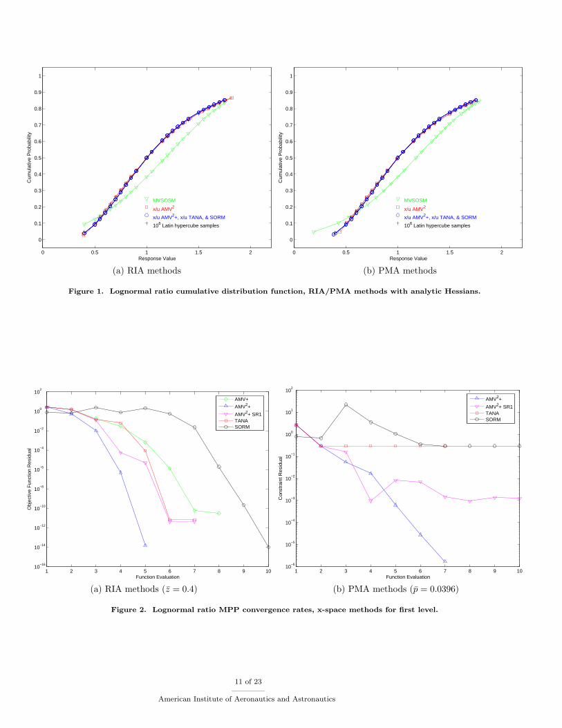
For RIA, 24 response levels (.4, .5, .55, .6, .65, .7, .75, .8, .85, .9, 1, 1.05, 1.15, 1.2, 1.25, 1.3, 1.35, 1.4, 1.5, 1.55, 1.6,1.65, 1.7, and 1.75) are mapped into the corresponding cumulative probability levels using first-order (for MVSOSMand AMV2) or second-order (for AMV2+, TANA, and SORM) integrations. For PMA, these 24 probability levels (thefully converged first-order or second-order results from RIA FORM/SORM) are mapped back into the original responselevels. As described in Section II.B, second-order PMA with prescribed probability levels involves the use of updatingschemes for β̄ in Eq. 16 and is the more challenging PMA case. Tables 1 and 3 show the computational results for eachof the primary RIA and PMA method variants using analytic limit state gradients and Hessians, and Tables 2 and 4show the computational results for RIA and PMA with AMV2+ using either numerical Hessians or quasi-Newton Hessianupdates. Duplicate function evaluations (detected by DAKOTA’s evaluation cache) are not included in the totals, anAMV2+/TANA convergence tolerance of ‖ u(k+1) − u(k) ‖2 < 10−4 is used to give comparable accuracy to the SORMconverged results, and an asterisk (∗) is used to indicate when one or more levels fails to converge to full accuracy. TheRIA p error norms and PMA z error norms are measured relative to the corresponding fully-converged FORM or SORMresults. That is, the inherent reliability analysis errors (e.g., RIA SORM p error norm of 0.05469 and PMA SORM zerror norm of 0.03775) relative to a Latin Hypercube reference solution of 106 samples are not included in order to avoidobscuring the relative errors. Figure 1 overlays the computed CDF values for each of the eight primary method variantscorresponding to Tables 1 and 3 as well as the Latin Hypercube reference solution (any unconverged CDF values, asdenoted by ∗ in the tables, are omitted for clarity). Figure 2 displays the convergence rates for different x-space MPPsearch methods in converging to the first RIA or PMA level.

It is evident that, relative to the fully-converged SORM results, MVSOSM has relatively poor accuracy across thefull range. AMV2 is reasonably accurate over the full range, although with mild offsets from the target response lev-els, and AMV2+ and TANA have full accuracy with reductions in expense (on average) relative to SORM. For thisproblem, AMV2+ with analytic Hessians and TANA are comparable, and x-space AMV2+ is the top performer. Whenapproximating Hessians for AMV2+, numerical Hessians are accurate although too expensive to be competitive, whereasSR1 quasi-Newton updates are accurate, competitive, and superior to BFGS updates (it is more important to accurately

9 of 23


Table 1. RIA results for lognormal ratio problem using analytic Hessians.

RIA SQP Function Evals NIP Function Evals CDF p Target z

Approach (val/grad/Hessian) (val/grad/Hessian) Error Norm Offset Norm

MVSOSM 1 (1/1/1) 1 (1/1/1) 0.3683 0.0

x-space AMV2 26 (26/1/1) 26 (26/1/1) 0.01369 0.1353

u-space AMV2 26* (26/1/1) 26 (26/1/1) 0.02438 0.1049

x-space AMV2+ 70 (70/69/69) 75 (75/74/74) 0.0 0.0

u-space AMV2+ 102 (102/101/101) 108 (108/107/107) 0.0 0.0

x-space TANA 83 (83/82/24) 85 (85/84/24) 0.0 0.0

u-space TANA 86 (86/85/24) 86 (86/85/24) 0.0 0.0

SORM 330 (306/305/24) 123 (99/98/24) 0.0 0.0

Table 2. RIA results for lognormal ratio problem using numerical Hessians (NH) and quasi-Hessians (QH).



x-space AMV2+ NH 217 (73/216/0) 223 (75/222/0) 1.657e-6 0.0

u-space AMV2+ NH 304 (102/303/0) 322 (108/321/0) 1.806e-6 0.0

x-space AMV2+ QH SR1 78 (78/77/0) 84 (84/83/0) 0.001063 0.0

u-space AMV2+ QH SR1 98 (98/97/0) 105 (105/104/0) 5.731e-7 0.0

x-space AMV2+ QH BFGS 147 (147/146/0) 123 (123/122/0) 1.073e-4 0.0

u-space AMV2+ QH BFGS 163 (163/162/0) 139 (139/138/0) 4.530e-5 0.0

Table 3. PMA results for lognormal ratio problem using analytic Hessians.

PMA SQP Function Evals NIP Function Evals CDF z Target p


MVSOSM 1 (1/1/1) 1 (1/1/1) 0.6277 0.0

x-space AMV2 26 (26/1/1) 26 (26/1/1) 0.4024 0.008609

u-space AMV2 26 (26/1/1) 26 (26/1/1) 0.04915 0.008423

x-space AMV2+ 77 (77/76/76) 80 (80/79/79) 0.0 0.0

u-space AMV2+ 92 (92/91/91) 112 (112/111/111) 0.0 0.0

x-space TANA 135* (135/134/24) 135* (135/134/24) 0.01869 0.007251

u-space TANA 111* (111/110/24) 115* (115/114/24) 0.01869 0.007251

SORM 698* (698/697/697) 106* (106/105/105) 0.01902 0.007701

Table 4. PMA results for lognormal ratio problem using numerical Hessians (NH) and quasi-Hessians (QH).



x-space AMV2+ NH 229 (77/228/0) 238 (80/237/0) 7.460e-6 4.716e-6

u-space AMV2+ NH 274 (92/273/0) 334 (112/333/0) 1.012e-5 6.627e-6

x-space AMV2+ QH SR1 143 (143/142/0) 146 (146/145/0) 0.002518 3.604e-4

u-space AMV2+ QH SR1 178 (178/177/0) 167 (167/166/0) 0.001099 7.716e-4

x-space AMV2+ QH BFGS 169 (169/168/0) 172 (172/171/0) 0.1470 0.09317

u-space AMV2+ QH BFGS 208 (208/207/0) 219 (219/218/0) 0.4932 0.4104

10 of 23


0 0.5 1 1.5 2

0

0.1

0.2

0.3

0.4

0.5

0.6

0.7

0.8

0.9

1

Response Value

Cum

ulat

ive

Pro

babi

lity

MVSOSM

x/u AMV2

x/u AMV2+, x/u TANA, & SORM

106 Latin hypercube samples

0 0.5 1 1.5 2

0

0.1

0.2

0.3

0.4

0.5

0.6

0.7

0.8

0.9

1

Response Value

Cum

ulat

ive

Pro

babi

lity

MVSOSM

x/u AMV2



(a) RIA methods (b) PMA methods

Figure 1. Lognormal ratio cumulative distribution function, RIA/PMA methods with analytic Hessians.

1 2 3 4 5 6 7 8 9 1010

−16

10−14

10−12

10−10

10−8

10−6

10−4

10−2

100

102

Obj

ectiv

e F

unct

ion

Res

idua

l

Function Evaluation

AMV+

AMV2+

AMV2+ SR1TANASORM

1 2 3 4 5 6 7 8 9 1010

−6

10−5

10−4

10−3

10−2

10−1

100

101

102

Con

stra

int R

esid

ual

Function Evaluation

AMV2+

AMV2+ SR1TANASORM

(a) RIA methods (z̄ = 0.4) (b) PMA methods (p̄ = 0.0396)

Figure 2. Lognormal ratio MPP convergence rates, x-space methods for first level.

11 of 23


estimate curvature than to retain positive definiteness). For second-order PMA, the AMV2+ approaches consistently findthe correct solution, whereas SORM and TANA approaches have minor convergence difficulties (for the first probabilitylevel only). When looking more closely at convergence for the first RIA and PMA levels, Figure 2 shows rates that arequadratic in nature for second-order RIA, but which are more linear in nature for the successful PMA methods due tothe p̄ → β̄ updates. Quadratic rates (and more consistent convergence) would be expected for PMA with prescribed β̄levels. Finally, optimizer selection has a large effect when not employing approximations, and the NIP option can be seento significantly outperform the SQP option and remain competitive with the approximation-based approaches.

In comparison with first-order method performance presented in Ref. 11, most of the new second-order methods showsignificant improvement. With the addition of analytic Hessians, AMV2 shows improved accuracy (e.g., a 5x reductionin RIA z offset error on average) and AMV2+ shows faster convergence (e.g., a 35% reduction in function evaluationsfor x-space AMV2+). More importantly for practical applications, quasi-Newton SR1 x-space AMV2+ shows a 24%reduction in expense over first-order AMV+ with no additional data requirements.

B. Short column

This test problem involves the plastic analysis and design of a short column with rectangular cross section (width b anddepth h) having uncertain material properties (yield stress Y ) and subject to uncertain loads (bending moment M andaxial force P ).20 The limit state function is defined as:

g(x) = 1 −4M

bh2Y−

P 2

b2h2Y 2(55)

The distributions for P , M , and Y are Normal(500, 100), Normal(2000, 400), and Lognormal(5, 0.5), respectively, witha correlation coefficient of 0.5 between P and M (uncorrelated otherwise). The nominal values for b and h are 5 and 15,respectively.


For RIA, 43 response levels (-9.0, -8.75, -8.5, -8.0, -7.75, -7.5, -7.25, -7.0, -6.5, -6.0, -5.5, -5.0, -4.5, -4.0, -3.5, -3.0, -2.5,-2.0, -1.9, -1.8, -1.7, -1.6, -1.5, -1.4, -1.3, -1.2, -1.1, -1.0, -0.9, -0.8, -0.7, -0.6, -0.5, -0.4, -0.3, -0.2, -0.1, 0.0, 0.05, 0.1, 0.15,0.2, 0.25) are mapped into the corresponding cumulative probability levels using first-order (for MVSOSM and AMV2) orsecond-order (for AMV2+, TANA, and SORM) integrations. For PMA, these 43 probability levels (the fully convergedfirst-order or second-order results from RIA FORM/SORM) are mapped back into the original response levels (usingupdating schemes in the second-order case for β̄(p̄)). Tables 5 and 7 show the computational results for each of theprimary RIA and PMA method variants using analytic limit state gradients and Hessians, and Tables 6 and 8 show thecomputational results for RIA and PMA with AMV2+ using either numerical Hessians or quasi-Newton Hessian updates.The RIA p error norms and PMA z error norms are measured relative to the corresponding fully-converged FORM orSORM results. That is, the inherent reliability analysis errors (e.g., RIA SORM p error norm of 0.01593 and PMA SORMz error norm of 0.2181) relative to a Latin Hypercube reference solution of 106 samples are omitted in order to avoidobscuring the relative errors. Figure 3 overlays the computed CDF values for each of the eight primary method variantscorresponding to Tables 5 and 7 as well as the Latin Hypercube reference solution.

Table 5. RIA results for short column problem using analytic Hessians.



MVSOSM 1 (1/1/1) 1 (1/1/1) 0.1127 0.0

x-space AMV2 45 (45/1/1) 45 (45/1/1) 0.002063 2.482

u-space AMV2 45 (45/1/1) 45 (45/1/1) 0.001410 2.031

x-space AMV2+ 125 (125/124/124) 131 (131/130/130) 0.0 0.0

u-space AMV2+ 122 (122/121/121) 130 (130/129/129) 0.0 0.0

x-space TANA 245 (245/244/43) 246 (246/245/43) 0.0 0.0

u-space TANA 296* (296/295/43) 278* (278/277/43) 6.982e-5 0.08014

SORM 669 (626/625/43) 219 (176/175/43)) 0.0 0.0

Relative to the fully-converged SORM results, MVSOSM is now reasonably accurate and greatly improved over thelognormal ratio test problem. AMV2 improves on the MVSOSM results, although with significant offsets in the RIA

12 of 23


Table 6. RIA results for short column problem using numerical Hessians (NH) and quasi-Hessians (QH).



x-space AMV2+ NH 481 (121/480/0) 521 (131/520/0) 4.156e-7 4.341e-8

u-space AMV2+ NH 513 (129/512/0) 517 (130/516/0) 4.195e-7 4.355e-8

x-space AMV2+ QH SR1 137 (137/136/0) 137 (137/136/0) 4.748e-5 4.372e-8

u-space AMV2+ QH SR1 139 (139/138/0) 138 (138/137/0) 1.164e-4 4.317e-8

x-space AMV2+ QH BFGS 290* (290/289/0) 227* (227/226/0) 1.001 12.70

u-space AMV2+ QH BFGS 294* (294/293/0) 240* (240/239/0) 1.121 13.85

Table 7. PMA results for short column problem using analytic Hessians.



MVSOSM 1 (1/1/1) 1 (1/1/1) 6.823 0.0

x-space AMV2 45 (45/1/1) 45 (45/1/1) 2.730 0.0

u-space AMV2 45 (45/1/1) 45 (45/1/1) 2.828 0.0

x-space AMV2+ 135 (135/134/134) 142 (142/141/141) 0.0 0.0

u-space AMV2+ 132 (132/131/131) 139 (139/138/138) 0.0 0.0

x-space TANA 293* (293/292/43) 272 (272/271/43) 0.04259 1.598e-4

u-space TANA 325* (325/324/43) 311* (311/310/43) 2.208 5.600e-4

SORM 535 (535/534/534) 191* (191/190/190) 2.410 6.522e-4

Table 8. PMA results for short column problem using numerical Hessians (NH) and quasi-Hessians (QH).



x-space AMV2+ NH 537 (135/536/0) 565 (142/564/0) 5.020e-6 7.556e-8

u-space AMV2+ NH 525 (132/524/0) 553 (139/552/0) 4.628e-6 1.101e-7

x-space AMV2+ QH SR1 255* (255/254/0) 252 (252/251/0) 0.004965 5.924e-5

u-space AMV2+ QH SR1 252 (252/251/0) 250 (250/249/0) 0.08599 2.093e-4

x-space AMV2+ QH BFGS 336* (336/335/0) 345* (345/344/0) 0.3979 6.133e-4

u-space AMV2+ QH BFGS 316* (316/315/0) 342* (342/341/0) 0.2178 0.003301

13 of 23


−10 −8 −6 −4 −2 0 2

0

0.1

0.2

0.3

0.4

0.5

0.6

0.7

0.8

0.9

1

Response Value

Cum

ulat

ive

Pro

babi

lity

MVSOSM

x/u AMV2



−10 −8 −6 −4 −2 0 2

0

0.1

0.2

0.3

0.4

0.5

0.6

0.7

0.8

0.9

1

Response Value

Cum

ulat

ive

Pro

babi

lity

MVSOSM

x/u AMV2



(a) RIA methods (b) PMA methods

Figure 3. Short column cumulative distribution function, RIA/PMA methods with analytic Hessians.

case from the target response levels. In the RIA case, AMV2+ and TANA have full accuracy and AMV2+ with analyticHessians reduces expense by a factor of 2.1 on average in comparison to TANA and by a factor of 3.5 on average incomparison to SORM. For PMA, AMV2+ with analytic Hessians is both the most robust and the most efficient approach.For AMV2+ with approximated Hessians, SR1 updating is again the best approach.

In comparison with first-order AMV+ performance presented in Ref. 11, AMV2+ for RIA reduces function evaluationcounts by 36% with analytic Hessians and by 31% in the quasi-Newton SR1 case, on average. For PMA, where the second-order case is more challenging than the first-order case in converging to a prescribed p̄, AMV2+ reduces function evaluationcounts by 27% for PMA with analytic Hessians, but increases function evaluation counts by 34% in the quasi-NewtonSR1 case, on average.

2. Reliability-based design optimization

The short column example problem is also amenable to RBDO. An objective function of cross-sectional area and a targetreliability index of 2.5 are used in the design problem:

min bh

s.t. β ≥ 2.5

5.0 ≤ b ≤ 15.0

15.0 ≤ h ≤ 25.0 (56)

It is important to note that only a single response/probability mapping is needed for each uncertainty analysis (instead ofthe 43 used previously in generating a full CDF). As is evident from the UQ results shown in Figure 3, the nominal designof (b, h) = (5, 15) is infeasible (p(g ≤ 0) > 0.9) and the optimization must add material to obtain the target reliability atthe optimal design (b, h) = (8.669, 25.00). Eq. 56 corresponds to an RIA z̄ → β approach, whereas an RIA z̄ → p approachwould constrain p and PMA β̄ → z and p̄ → z approaches would constrain z. The second-order cumulative probabilitycorresponding to the optimal solution (used for level specification in PMA p̄→ z and for the constraint allowable in RIAz̄ → p) is p(g ≤ 0) = 0.005992, which is relatively close to the corresponding first-order probability of 0.006210.

Table 9 shows the results for fully-analytic bi-level second-order RBDO employing the gradient expressions for z,β, and p (Eqs. 44-45 and 47). Constraint violations are raw norms (not normalized by allowable). SQP is used foroptimization at both levels. In this case, MVSOSM and AMV2 variants for RIA/PMA RBDO are not allowed, since thesensitivity expressions require a fully-converged MPP. The function evaluation tabulations indicate that AMV2+-basedRBDO significantly outperforms SORM-based RBDO by a factor of 6.2 on average. Applying reliability constraints is morecomputationally efficient than applying probability constraints in the RIA RBDO formulation of Eq. 42 (expense reducedby a factor of 2.0 on average), since β tends to be more linear and well-scaled than p; however, only the formulations

14 of 23


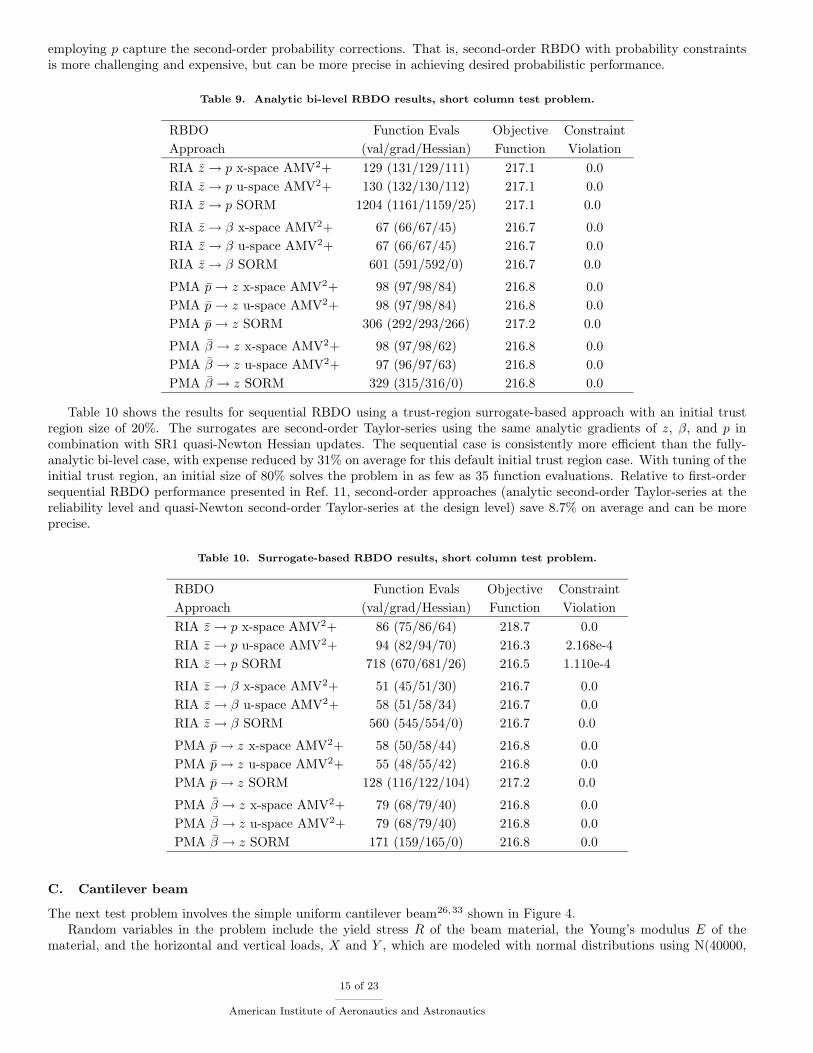
employing p capture the second-order probability corrections. That is, second-order RBDO with probability constraintsis more challenging and expensive, but can be more precise in achieving desired probabilistic performance.

Table 9. Analytic bi-level RBDO results, short column test problem.

RBDO Function Evals Objective Constraint

Approach (val/grad/Hessian) Function Violation

RIA z̄ → p x-space AMV2+ 129 (131/129/111) 217.1 0.0

RIA z̄ → p u-space AMV2+ 130 (132/130/112) 217.1 0.0

RIA z̄ → p SORM 1204 (1161/1159/25) 217.1 0.0

RIA z̄ → β x-space AMV2+ 67 (66/67/45) 216.7 0.0

RIA z̄ → β u-space AMV2+ 67 (66/67/45) 216.7 0.0

RIA z̄ → β SORM 601 (591/592/0) 216.7 0.0

PMA p̄→ z x-space AMV2+ 98 (97/98/84) 216.8 0.0

PMA p̄→ z u-space AMV2+ 98 (97/98/84) 216.8 0.0

PMA p̄→ z SORM 306 (292/293/266) 217.2 0.0

PMA β̄ → z x-space AMV2+ 98 (97/98/62) 216.8 0.0

PMA β̄ → z u-space AMV2+ 97 (96/97/63) 216.8 0.0

PMA β̄ → z SORM 329 (315/316/0) 216.8 0.0

Table 10 shows the results for sequential RBDO using a trust-region surrogate-based approach with an initial trustregion size of 20%. The surrogates are second-order Taylor-series using the same analytic gradients of z, β, and p incombination with SR1 quasi-Newton Hessian updates. The sequential case is consistently more efficient than the fully-analytic bi-level case, with expense reduced by 31% on average for this default initial trust region case. With tuning of theinitial trust region, an initial size of 80% solves the problem in as few as 35 function evaluations. Relative to first-ordersequential RBDO performance presented in Ref. 11, second-order approaches (analytic second-order Taylor-series at thereliability level and quasi-Newton second-order Taylor-series at the design level) save 8.7% on average and can be moreprecise.

Table 10. Surrogate-based RBDO results, short column test problem.



RIA z̄ → p x-space AMV2+ 86 (75/86/64) 218.7 0.0

RIA z̄ → p u-space AMV2+ 94 (82/94/70) 216.3 2.168e-4

RIA z̄ → p SORM 718 (670/681/26) 216.5 1.110e-4

RIA z̄ → β x-space AMV2+ 51 (45/51/30) 216.7 0.0

RIA z̄ → β u-space AMV2+ 58 (51/58/34) 216.7 0.0

RIA z̄ → β SORM 560 (545/554/0) 216.7 0.0

PMA p̄→ z x-space AMV2+ 58 (50/58/44) 216.8 0.0

PMA p̄→ z u-space AMV2+ 55 (48/55/42) 216.8 0.0

PMA p̄→ z SORM 128 (116/122/104) 217.2 0.0

PMA β̄ → z x-space AMV2+ 79 (68/79/40) 216.8 0.0

PMA β̄ → z u-space AMV2+ 79 (68/79/40) 216.8 0.0

PMA β̄ → z SORM 171 (159/165/0) 216.8 0.0

C. Cantilever beam

The next test problem involves the simple uniform cantilever beam26,33 shown in Figure 4.Random variables in the problem include the yield stress R of the beam material, the Young’s modulus E of the

material, and the horizontal and vertical loads, X and Y , which are modeled with normal distributions using N(40000,

15 of 23


L = 100”

w

tX

Y

Figure 4. Cantilever beam test problem.

2000), N(2.9E7, 1.45E6), N(500, 100), and N(1000, 100), respectively. Problem constants include L = 100 in. and D0 =2.2535 in. The constraints on beam response have the following analytic form:

stress =600

wt2Y +

600

w2tX ≤ R (57)

displacement =4L3

Ewt

√

(Y

t2)2 + (

X

w2)2 ≤ D0 (58)

or when scaled:

gS =stress

R− 1 ≤ 0 (59)

gD =displacement

D0− 1 ≤ 0 (60)


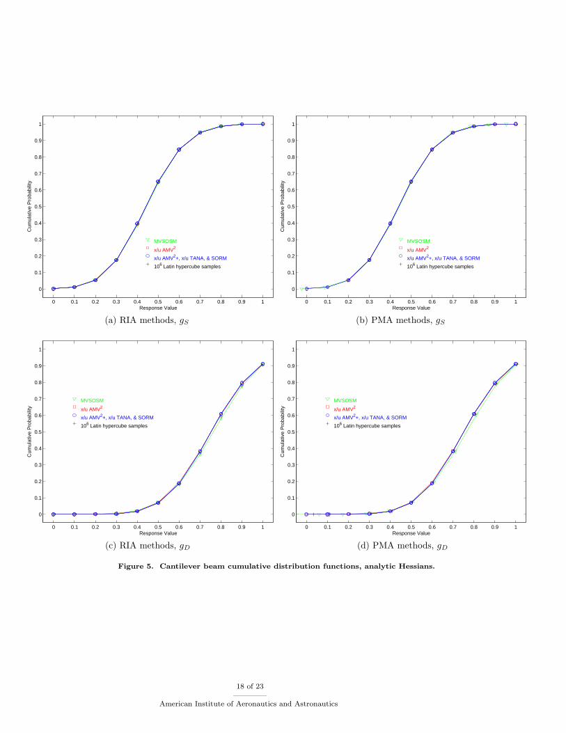
For RIA, 11 levels (0.0 to 1.0 in 0.1 increments) are employed for each limit state function (gS and gD) and are mappedinto the corresponding cumulative probability levels using first-order (for MVSOSM and AMV2) or second-order (forAMV2+, TANA, and SORM) integrations. For PMA, these probability levels (the fully converged first-order or second-order results from RIA FORM/SORM) are mapped back into the original response levels (using updating schemes in thesecond-order case for β̄(p̄)). Tables 11 and 13 show the computational results for each of the primary RIA and PMAmethod variants using analytic gradients and Hessians, and Tables 12 and 14 show the computational results for RIA andPMA with AMV2+ using either numerical Hessians or quasi-Newton Hessian updates. In this problem, since all uncertainvariables are normally distributed and uncorrelated, the x-space and u-space linearization approaches are equivalent. TheRIA p error norms and PMA z error norms are measured relative to the corresponding fully-converged FORM or SORMresults. That is, the inherent reliability analysis errors (e.g., RIA SORM p error norm of 0.02943 and PMA SORM zerror norm of 0.04198) relative to a Latin Hypercube reference solution of 106 samples are not included in order to avoidobscuring the relative errors. Figure 5 overlays the computed CDF values for each of the method variants as well as theLatin Hypercube reference solution (any unconverged CDF values as denoted by ∗ in the tables are omitted for clarity).

Table 11. RIA results for cantilever problem using analytic Hessians.



MVSOSM 1 (2/2/2) 1 (2/2/2) 0.04064 0.0

x-/u-space AMV2 23 (24/2/2) 23 (24/2/2) 8.763e-6 0.007661

x-/u-space AMV2+ 59 (60/60/60) 67 (68/68/68) 0.0 0.0

x-/u-space TANA 116 (117/117/22) 123 (124/124/22) 0.0 0.0

SORM 187 (166/164/22) 117 (96/94/22) 0.0 0.0

Relative to the fully-converged SORM results, MVSOSM and AMV2 are quite accurate for this problem. In the RIAcase, AMV2+ and TANA have full accuracy and AMV2+ with analytic Hessians outperforms TANA and SORM (reducesfunction evaluations by factors of 1.9 and 2.5, respectively). For PMA, AMV2+ with analytic Hessians is again the mostrobust and efficient approach. For AMV2+ with approximated Hessians, SR1 updating is again the best approach.

In comparison with first-order AMV+ performance presented in Ref. 11, AMV2+ for RIA reduces function evaluationcounts by 31% with analytic Hessians and by 16% in the quasi-Newton SR1 case, on average. For PMA, where convergingto a prescribed second-order p̄ is more challenging than the first-order case, AMV2+ reduces function evaluation counts

16 of 23


Table 12. RIA results for cantilever problem using numerical Hessians (NH) and quasi-Hessians (QH).



x-/u-space AMV2+ NH 270 (55/275/0) 335 (68/340/0) 1.202e-7 1.662e-7

x-/u-space AMV2+ QH SR1 75 (76/76/0) 78 (79/79/0) 0.001014 3.070e-6

x-/u-space AMV2+ QH BFGS 114 (115/115/0) 107* (108/108/0) 1.145 1.011

Table 13. PMA results for cantilever problem using analytic Hessians.



MVSOSM 1 (2/2/2) 1 (2/2/2) 0.1025 0.0

x-/u-space AMV2 23 (24/2/2) 23 (24/2/2) 0.4044 0.006347

x-/u-space AMV2+ 68 (69/69/69) 71 (72/72/72) 0.0 0.0

x-/u-space TANA 118 (119/119/22) 115 (116/116/22) 0.003029 4.137e-4

SORM 248* (249/247/247) 150* (151/149/149) 0.4176 0.006159

Table 14. PMA results for cantilever problem using numerical Hessians (NH) and quasi-Hessians (QH).



x-/u-space AMV2+ NH 340 (69/345/0) 355 (72/360/0) 2.152e-7 1.806e-8

x-/u-space AMV2+ QH SR1 102 (103/103/0) 108 (109/109/0) 0.01348 0.005450

x-/u-space AMV2+ QH BFGS 159* (160/160/0) 156* (157/157/0) 10.657 0.5833

17 of 23


0 0.1 0.2 0.3 0.4 0.5 0.6 0.7 0.8 0.9 1

0

0.1

0.2

0.3

0.4

0.5

0.6

0.7

0.8

0.9

1

Response Value

Cum

ulat

ive

Pro

babi

lity

MVSOSM

x/u AMV2



0 0.1 0.2 0.3 0.4 0.5 0.6 0.7 0.8 0.9 1

0

0.1

0.2

0.3

0.4

0.5

0.6

0.7

0.8

0.9

1

Response Value

Cum

ulat

ive

Pro

babi

lity

MVSOSM

x/u AMV2



(a) RIA methods, gS (b) PMA methods, gS

0 0.1 0.2 0.3 0.4 0.5 0.6 0.7 0.8 0.9 1

0

0.1

0.2

0.3

0.4

0.5

0.6

0.7

0.8

0.9

1

Response Value

Cum

ulat

ive

Pro

babi

lity

MVSOSM

x/u AMV2



0 0.1 0.2 0.3 0.4 0.5 0.6 0.7 0.8 0.9 1

0

0.1

0.2

0.3

0.4

0.5

0.6

0.7

0.8

0.9

1

Response Value

Cum

ulat

ive

Pro

babi

lity

MVSOSM

x/u AMV2



(c) RIA methods, gD (d) PMA methods, gD

Figure 5. Cantilever beam cumulative distribution functions, analytic Hessians.

18 of 23


by 10% for PMA with analytic Hessians, but increases function evaluation counts by 35% in the quasi-Newton SR1 case,on average.


The design problem is to minimize the weight (or, equivalently, the cross-sectional area) of the beam subject to thedisplacement and stress constraints. If the random variables are fixed at their means, the resulting deterministic designproblem (with constraints gS ≤ 0 and gD ≤ 0) has the solution (w, t) = (2.352, 3.326) with an objective function of 7.824.When seeking reliability levels of 3.0 for these constraints, the design problem becomes:

min wt

s.t. βD ≥ 3.0

βS ≥ 3.0

1.0 ≤ w ≤ 4.0

1.0 ≤ t ≤ 4.0 (61)

which has the solution (w, t) = (2.451, 3.884) with an objective function of 9.520. This formulation corresponds to anRIA z̄ → β approach, whereas an RIA z̄ → p approach would constrain p and PMA β̄ → z and p̄ → z approacheswould constrain z. The second-order complementary cumulative probabilities corresponding to the optimal solution (usedfor level specification in PMA p̄ → z and for the constraint allowable in RIA z̄ → p) are p(gS > 0) = 0.001350 andp(gD > 0) = 0.001145, which are equal and similar, respectively, to the corresponding first-order probabilities of 0.001350.

Table 15 shows the results for fully-analytic bi-level second-order RBDO employing the gradient expressions for z,β, and p (Eqs. 44-45 and 47). Constraint violations are raw norms (not normalized by allowable), and SQP is used foroptimization at both levels. AMV2+-based RBDO reduces expense relative to SORM-based RBDO by a factor of 2.9 onaverage. β-based formulations are again more computationally efficient, but lack the precision of second-order probabilityintegrations.

Table 15. Analytic bi-level RBDO results, cantilever test problem.



RIA z̄ → p x-/u-space AMV2+ 258 (279/312/279) 9.562 0.0

RIA z̄ → p SORM 625 (551/530/58) 9.562 0.0

RIA z̄ → β x-/u-space AMV2+ 183 (189/213/143) 9.520 0.0

RIA z̄ → β SORM 335 (326/320/0) 9.520 0.0

PMA p̄→ z x-/u-space AMV2+ 262 (278/302/278) 9.519 2.245e-4

PMA p̄→ z SORM 853 (849/833/789) 9.519 2.027e-4

PMA β̄ → z x-/u-space AMV2+ 208 (224/248/174) 9.521 0.0

PMA β̄ → z SORM 855 (851/835/0) 9.521 0.0

Table 16 shows the results for sequential RBDO using a trust-region surrogate-based approach with an initial trust re-gion size of 20%. The surrogates are again second-order Taylor-series using analytic gradients of z, β, and p in combinationwith SR1 quasi-Newton Hessian updates. The sequential case is more efficient than the fully-analytic bi-level case, withexpense reduced by 41% on average. With tuning of the initial trust region, an initial size of 10% solves the problem in asfew as 75 function evaluations. Relative to first-order sequential RBDO performance presented in Ref. 11, second-orderapproaches (analytic second-order Taylor-series at the reliability level and quasi-Newton second-order Taylor-series at thedesign level) save 29% on average and can be more precise.

D. Steel Column

The final test problem involves the trade-off between cost and reliability for a steel column.20 The cost is defined as

Cost = bd+ 5h (62)

where b, d, and h are the means of the flange breadth, flange thickness, and profile height, respectively. Nine uncorrelatedrandom variables are used in the problem to define the yield stress Fs (lognormal with µ/σ = 400/35 MPa), dead weight

19 of 23


Table 16. Surrogate-based RBDO results, cantilever test problem.



RIA z̄ → p x-/u-space AMV2+ 174 (163/202/163) 9.618 0.0

RIA z̄ → p SORM 324 (265/274/38) 9.534 2.570e-5

RIA z̄ → β x-/u-space AMV2+ 118 (110/134/83) 9.521 0.0

RIA z̄ → β SORM 213 (198/205/0) 9.521 0.0

PMA p̄→ z x-/u-space AMV2+ 134 (125/148/125) 9.521 0.0

PMA p̄→ z SORM 515 (501/508/480) 9.521 0.0

PMA β̄ → z x-/u-space AMV2+ 102 (95/116/69) 9.522 2.525e-3

PMA β̄ → z SORM 558 (549/549/0) 9.522 0.0

load P1 (normal with µ/σ = 500000/50000 N), variable load P2 (gumbel with µ/σ = 600000/90000 N), variable load P3

(gumbel with µ/σ = 600000/90000 N), flange breadth B (lognormal with µ/σ = b/3 mm), flange thickness D (lognormalwith µ/σ = d/2 mm), profile height H (lognormal with µ/σ = h/5 mm), initial deflection F0 (normal with µ/σ = 30/10mm), and youngs modulus E (weibull with µ/σ = 21000/4200 MPa). The limit state has the following analytic form:

g = Fs − P

(

1

2BD+

F0

BDH

Eb

Eb − P

)

(63)

where

P = P1 + P2 + P3 (64)

Eb =π2EBDH2

2L2(65)

and the column length L is 7500 mm.


This design problem demonstrates design variable insertion into random variable distribution parameters through thedesign of the mean flange breadth, flange thickness, and profile height. The following RBDO formulation maximizes thereliability subject to a cost constraint:

max β

s.t. Cost ≤ 4000.

200.0 ≤ b ≤ 400.0

10.0 ≤ d ≤ 30.0

100.0 ≤ h ≤ 500.0 (66)

which has the solution (b, d, h) = (200.0, 17.50, 100.0) with a maximal reliability of 3.132. This corresponds to an RIAz̄ → β approach, where the RIA z̄ → p approach would minimize p and the PMA β̄ → z and p̄ → z approaches wouldmaximize z. The second-order cumulative probability corresponding to the optimal solution (used for PMA p̄ → z) isp(g ≤ 0) = 0.001309, which differs significantly from the corresponding first-order probability of 8.678e-4.

Table 17 shows the results for fully-analytic bi-level second-order RBDO employing the gradient expressions for z, β,and p (Eqs. 47-51). Constraint violations are raw norms (not normalized by allowable), and SQP and NIP are used foroptimization at the design and MPP search levels, respectively. With the use of NIP at the reliability level, the benefitsof AMV2+-based RBDO relative to SORM-based RBDO are less pronounced, with average reductions in expense of 17%on average. β-based formulations are again more computationally efficient (although less precise with the omission ofsecond-order probability integrations) and are also more robust since second-order PMA with p̄ had some difficulty: whileit located the correct optimal solution, the final response level (marked with “*”) was incorrect due to inaccurate p̄→ β̄inversions.

Table 18 shows the results for sequential RBDO using a trust-region surrogate-based approach with an initial trustregion size of 20%. The surrogates are second-order Taylor-series using analytic gradients of z, β, and p in combination

20 of 23


Table 17. Analytic bi-level RBDO results, steel column test problem.



RIA z̄ → p x-space AMV2+ 315 (315/272/229) 0.001309 0.0

RIA z̄ → p u-space AMV2+ 311 (311/268/225) 0.001309 0.0

RIA z̄ → p SORM 322 (279/236/43) 0.001309 0.0

RIA z̄ → β x-space AMV2+ 90 (90/78/54) 3.132 0.0

RIA z̄ → β u-space AMV2+ 88 (88/76/52) 3.132 0.0

RIA z̄ → β SORM 90 (90/78/0) 3.132 0.0

PMA p̄→ z x-space AMV2+ 52 (52/45/38) 0.001481 0.0

PMA p̄→ z u-space AMV2+ 53 (53/46/39) 0.001481 0.0

PMA p̄→ z SORM 67 (67/60/53) 7.401* 0.0

PMA β̄ → z x-space AMV2+ 49 (49/42/28) 0.005223 0.0

PMA β̄ → z u-space AMV2+ 48 (48/41/27) 0.005223 0.0

PMA β̄ → z SORM 83 (83/76/0) 0.005221 0.0

with SR1 quasi-Newton Hessian updates. The sequential and bi-level cases are more competitive in this problem, butsequential is still more efficient with expense reduced by 13% on average. Second-order PMA with p̄ again had difficulty.With tuning of the initial trust region, an initial size of 80% solves the problem in as few as 45 function evaluations.

Table 18. Surrogate-based RBDO results, steel column test problem.



RIA z̄ → p x-space AMV2+ 62 (62/49/44) 0.001309 0.0

RIA z̄ → p u-space AMV2+ 62 (62/49/44) 0.001309 0.0

RIA z̄ → p SORM 81 (72/59/9) 0.001309 0.0

RIA z̄ → β x-space AMV2+ 67 (67/52/37) 3.132 0.0

RIA z̄ → β u-space AMV2+ 67 (67/52/37) 3.132 0.0

RIA z̄ → β SORM 78 (78/63/0) 3.132 0.0

PMA p̄→ z x-space AMV2+ 64 (64/49/44) 0.001500 0.0

PMA p̄→ z u-space AMV2+ 63 (63/48/43) 0.001500 0.0

PMA p̄→ z SORM 86 (86/71/66) 7.401* 0.0

PMA β̄ → z x-space AMV2+ 62 (62/47/32) 0.005223 0.0

PMA β̄ → z u-space AMV2+ 60 (60/45/30) 0.005223 0.0

PMA β̄ → z SORM 102 (102/87/0) 0.005223 0.0

V. Conclusions

The effectiveness of first-order approximations, both in limit state linearization within reliability analysis and insurrogate-based RBDO, has led to additional work in second-order approximations which seek improved accuracy inprobability integrations and improved computational efficiency through accelerated convergence rates.

This paper explores second-order RIA and PMA formulations using various limit state approximation (MVSOSM, x-/u-space AMV2, x-/u-space AMV2+, x-/u-space TANA, and SORM), probability integration (first-order or second-order),Hessian approximation (finite difference, BFGS, or SR1), and MPP optimization algorithm (SQP or NIP) selections.When performing the p̄ → z PMA mapping, an updating scheme for β̄ is used to account for changes in the limit statecurvature.

Reliability analysis results for the lognormal ratio, short column, and cantilever test problems indicate several trends.

21 of 23


MVSOSM and AMV2 are significantly less expensive than AMV2+, TANA, and SORM, but come with correspondingreductions in accuracy. In combination, these methods provide a useful spectrum of accuracy and expense that allowthe computational effort to be balanced with the precision desired for particular applications. In addition, support forforward and inverse mappings (RIA and PMA) provide the flexibility to support different UQ analysis needs. The AMV2+approaches were shown to be the most efficient for second-order RIA analysis and both the most robust and the mostefficient for second-order PMA analysis with prescribed probability levels. Analytic Hessians were highly effective inAMV2+, but since they are often unavailable in practical applications, finite-difference numerical Hessians and quasi-Newton Hessian approximations were also demonstrated, with SR1 quasi-Newton updates being shown to be sufficientlyaccurate and competitive with analytic Hessian performance. Relative to first-order AMV+ performance, AMV2+ withanalytic Hessians had consistently superior efficiency, and AMV2+ with quasi-Newton Hessians had improved performancein most cases (it was more expensive than AMV+ only when a more challenging second-order p̄ problem was being solved).

An important question is how Taylor-series based limit state approximations (such as AMV+ and AMV2+) canfrequently outperform the best general-purpose optimizers (such as SQP and NIP). The answer likely lies in the exploitationof the structure of the RIA and PMA MPP problems. By approximating the limit state but retaining uT u explicitly,specific problem structure knowledge is utilized in formulating a mixed surrogate/direct approach.

These reliability analysis capabilities provide a substantial foundation for RBDO formulations, and bi-level and sequen-tial RBDO approaches have been investigated. Both approaches have utilized analytic gradients for z, β, and second-orderp with respect to augmented and inserted design variables, and sequential RBDO has additionally utilized a trust-regionsurrogate-based approach to manage the extent of the second-order Taylor-series approximations.

RBDO results for the short column, cantilever, and steel column test problems build on the reliability analysis trends.In bi-level and sequential RBDO, the AMV2+ approaches were consistently more efficient than the SORM-based ap-proaches. In addition, sequential RBDO approaches demonstrated computational savings over the corresponding bi-levelRBDO approaches. The combination of sequential RBDO using AMV2+ was the most effective of all of the approaches.With initial trust region size tuning, RBDO computational expense for these test problems was shown to be as low asapproximately 40 function evaluations per limit state (35 for a single limit state in short column, 75 for two limit statesin cantilever, and 45 for a single limit state in steel column). Second-order RBDO with probability constraints was shownto be more challenging and expensive, but could be more precise in achieving the desired probabilistic performance.

Overall, second-order reliability analysis and design approaches appear to serve multiple synergistic needs. The sameHessian information that allows for more accurate probability integrations can also be applied to making MPP solutionsmore efficient and more robust. Conversely, limit state curvature information accumulated during an MPP search canbe reused to improve the accuracy of probability estimates. Future algorithmic directions include sequential RBDO withmixed surrogate and direct models (for probabilistic and deterministic components, respectively). Initial deployment ofthese algorithmic capabilities within Sandia labs is targeting probabilistic analysis and design of micro-electro-mechanicalsystems (MEMS).

VI. Acknowledgments

The authors would like to express their thanks to the Sandia Computer Science Research Institute (CSRI) for supportof this collaborative work between Sandia National Laboratories and Vanderbilt University.

References

1Adams, B.M., Eldred, M.S., Wittwer, J.W., and Massad, J.E., Reliability-Based Design Optimization for Shape Design of Compliant Micro-Electro-Mechanical Systems, to appear in Proceedings of the 11th AIAA/ISSMO Multidisciplinary Analysis and Optimization Conference,Portsmouth, VA, Sept. 6-8, 2006.

2Agarwal, H., Renaud, J.E., Lee, J.C., and Watson, L.T., A Unilevel Method for Reliability Based Design Optimization, paper AIAA-2004-2029 in Proceedings of the 45th AIAA/ASME/ASCE/AHS/ASC Structures, Structural Dynamics, and Materials Conference, Palm Springs,CA, April 19-22, 2004.

3Allen, M. and Maute, K., Reliability-based design optimization of aeroelastic structures, Struct. Multidiscip. O., Vol. 27, 2004, pp. 228-242.4Box, G.E.P. and Cox, D.R., An Analysis of Transformations, J. Royal Stat. Soc., Series B, Vol. 26, 1964, pp. 211-252.5Breitung, K., Asymptotic approximation for multinormal integrals, J. Eng. Mech., ASCE, Vol. 110, No. 3, 1984, pp. 357-366.6Chen, X., and Lind, N.C., Fast Probability Integration by Three-Parameter Normal Tail Approximation, Struct. Saf., Vol. 1, 1983, pp.

269-276.7Der Kiureghian, A. and Liu, P.L., Structural Reliability Under Incomplete Probability Information, J. Eng. Mech., ASCE, Vol. 112, No.

1, 1986, pp. 85-104.8Du, X. and Chen, W., Sequential Optimization and Reliability Assessment Method for Efficient Probabilistic Design, J. Mech. Design,

Vol. 126, 2004, pp.225-233.9Eldred, M.S., Giunta, A.A., Wojtkiewicz, S.F., Jr., and Trucano, T.G., Formulations for Surrogate-Based Optimization Under Uncertainty,

22 of 23


paper AIAA-2002-5585 in Proceedings of the 9th AIAA/ISSMO Symposium on Multidisciplinary Analysis and Optimization, Atlanta, GA,Sept. 4-6, 2002.

10Eldred, M.S., Giunta, A.A., van Bloemen Waanders, B.G., Wojtkiewicz, S.F., Jr., Hart, W.E., and Alleva, M.P., DAKOTA, A MultilevelParallel Object-Oriented Framework for Design Optimization, Parameter Estimation, Uncertainty Quantification, and Sensitivity Analysis.Version 3.1 Users Manual. Sandia Technical Report SAND2001-3796, Revised April 2003, Sandia National Laboratories, Albuquerque, NM.

11Eldred, M.S., Agarwal, H., Perez, V.M., Wojtkiewicz, S.F., Jr., and Renaud, J.E., Investigation of Reliability Method Formulations inDAKOTA/UQ, (to appear) Structure & Infrastructure Engineering: Maintenance, Management, Life-Cycle Design & Performance, Taylor &Francis Group.

12Fadel, G.M., Riley, M.F., and Barthelemy, J.-F.M., Two Point Exponential Approximation Method for Structural Optimization, Struc-tural Optimization, Vol. 2, No. 2, 1990, pp. 117-124.

13Gill, P.E., Murray, W., Saunders, M.A., and Wright, M.H., User’s Guide for NPSOL 5.0: A Fortran Package for Nonlinear Programming,System Optimization Laboratory, Technical Report SOL 86-1, Revised July 1998, Stanford University, Stanford, CA.

14Giunta, A.A. and Eldred, M.S., Implementation of a Trust Region Model Management Strategy in the DAKOTA Optimization Toolkit,paper AIAA-2000-4935 in Proceedings of the 8th AIAA/USAF/NASA/ISSMO Symposium on Multidisciplinary Analysis and Optimization,Long Beach, CA, September 6-8, 2000.

15Haldar, A. and Mahadevan, S., Probability, Reliability, and Statistical Methods in Engineering Design, 2000 (Wiley: New York).16Hohenbichler, M. and Rackwitz, R., Sensitivity and importance measures in structural reliability, Civil Eng. Syst., Vol. 3, 1986, pp.

203-209.17Hohenbichler, M. and Rackwitz, R., Improvement of second-order reliability estimates by importance sampling, J. Eng. Mech., ASCE,

Vol. 114, No. 12, 1988, pp. 2195-2199.18Hong, H.P., Simple Approximations for Improving Second-Order Reliability Estimates, J. Eng. Mech., ASCE, Vol. 125, No. 5, 1999, pp.

592-595.19Karamchandani, A. and Cornell, C.A., Sensitivity estimation within first and second order reliability methods, Struct. Saf., Vol. 11,

1992, pp. 95-107.20Kuschel, N. and Rackwitz, R., Two Basic Problems in Reliability-Based Structural Optimization, Math. Method Oper. Res., Vol. 46,

1997, pp.309-333.21Meza, J.C., OPT++: An Object-Oriented Class Library for Nonlinear Optimization, Sandia Technical Report SAND94-8225, Sandia

National Laboratories, Livermore, CA, March 1994.22Nocedal, J., and Wright, S.J., Numerical Optimization, Springer, New York, 1999.23Rackwitz, R., and Fiessler, B., Structural Reliability under Combined Random Load Sequences, Comput. Struct., Vol. 9, 1978, pp.

489-494.24Rackwitz, R., Optimization and risk acceptability based on the Life Quality Index, Struct. Saf., Vol. 24, 2002, pp. 297-331.25Rosenblatt, M., Remarks on a Multivariate Transformation, Ann. Math. Stat., Vol. 23, No. 3, 1952, pp. 470-472.26Sues, R., Aminpour, M. and Shin, Y., Reliability-Based Multidisciplinary Optimization for Aerospace Systems, paper AIAA-2001-1521

in Proceedings of the 42rd AIAA/ASME/ASCE/AHS/ASC Structures, Structural Dynamics, and Materials Conference, Seattle, WA, April16-19, 2001.

27Tu, J., Choi, K.K., and Park, Y.H., A New Study on Reliability-Based Design Optimization, J. Mech. Design, Vol. 121, 1999, pp.557-564.28Wang, L. and Grandhi, R.V., Efficient Safety Index Calculation for Structural Reliability Analysis, Comput. Struct., Vol. 52, No. 1, 1994,

pp. 103-111.29Wojtkiewicz, S.F., Jr., Eldred, M.S., Field, R.V., Jr., Urbina, A., and Red-Horse, J.R., A Toolkit For Uncertainty Quantification In Large

Computational Engineering Models, paper AIAA-2001-1455 in Proceedings of the 42nd AIAA/ASME/ASCE/AHS/ASC Structures, StructuralDynamics, and Materials Conference, Seattle, WA, April 16-19, 2001.

30Wu, Y.-T., and Wirsching, P.H., A new algorithm for structural reliability estimation, J. Eng. Mech., ASCE, Vol. 113, 1987, pp.1319-1336.

31Wu, Y.-T., Millwater, H.R., and Cruse, T.A., Advanced Probabilistic Structural Analysis Method for Implicit Performance Functions,AIAA J., Vol. 28, No. 9, 1990, pp. 1663-1669.

32Wu, Y.-T., Computational Methods for Efficient Structural Reliability and Reliability Sensitivity Analysis, AIAA J., Vol. 32, No. 8,1994, pp. 1717-1723.

33Wu, Y.-T., Shin, Y., Sues, R., and Cesare, M., Safety-Factor Based Approach for Probability-Based Design Optimization, paper AIAA-2001-1522 in Proceedings of the 42rd AIAA/ASME/ASCE/AHS/ASC Structures, Structural Dynamics, and Materials Conference, Seattle,WA, April 16-19, 2001.

34Xu, S., and Grandhi, R.V., Effective Two-Point Function Approximation for Design Optimization, AIAA J., Vol. 36, No. 12, 1998, pp.2269-2275.

35Zou, T., Mahadevan, S., and Rebba, R., Computational Efficiency in Reliability-Based Optimization, Proceedings of the 9th ASCESpecialty Conference on Probabilistic Mechanics and Structural Reliability, Albuquerque, NM, July 26-28, 2004.

23 of 23


Second-Order Reliability Formulations in DAKOTA/UQ · Sequential and unilevel methods seek to...

Documents

Transcript of Second-Order Reliability Formulations in DAKOTA/UQ · Sequential and unilevel methods seek to...