Second-order inelastic dynamic analysis of 3-D steel...

International Journal of Solids and Structures 43 (2006) 1693–1709

www.elsevier.com/locate/ijsolstr

Second-order inelastic dynamic analysis of 3-D steel frames

Seung-Eock Kim *, Cuong Ngo-Huu, Dong-Ho Lee

Department of Civil and Environmental Engineering/Construction Tech. Research Institute, Sejong University, 98 Kunja-dong,

Kwangjin-ku, Seoul, 143-747, South Korea

Received 30 November 2004; received in revised form 19 May 2005Available online 20 July 2005

Abstract

This paper presents a reliable numerical procedure for nonlinear time-history analysis of three-dimensional steelframes subjected to dynamic loads. Geometric nonlinearities of member (P-d) and frame (P-D) are taken into accountby the use of stability functions in framed stiffness matrix formulation. The gradual yielding along the member lengthand over the cross-section is included by using a tangent modulus concept and a softening plastic hinge model based ona modified version of Orbison yield surface. A computer program utilizing the average acceleration method for the inte-gration scheme is developed to numerically solve the equation of motion of framed structure formulated in an incre-mental form. The results of several numerical examples are compared with those derived from using beam elementmodel of ABAQUS program to illustrate the accuracy and the computational efficiency of the proposed procedure.� 2005 Elsevier Ltd. All rights reserved.

Keywords: Dynamic analysis; Geometric and material nonlinearities; Plastic hinges; Stability functions; Three-dimensional steelframes

1. Introduction

The second-order inelastic static analysis of three-dimensional steel frames has been studied extensivelyin recent years together with the rapid development of computer technology. The finite element methodusing the interpolation functions and the fiber approach for representing the second-order effect and thespread of plasticity is performed by Izzuddin and Smith (1996), Teh and Clark (1999), and Jiang et al.(2002). Although it can include the interaction between normal and shear stresses and its solution is con-sidered to be accurate, it has not been applied widely for daily use in office engineering design because of its

0020-7683/$ - see front matter � 2005 Elsevier Ltd. All rights reserved.doi:10.1016/j.ijsolstr.2005.06.018

* Corresponding author. Tel.: +82 2 3408 3291; fax: +82 2 3408 3332.E-mail address: [email protected] (S.-E. Kim).

mailto:[email protected]

1694 S.-E. Kim et al. / International Journal of Solids and Structures 43 (2006) 1693–1709

highly computational cost. A more simple and efficient method is the beam-column method using stabilityfunctions and refined plastic-hinge approach proposed by Liew et al. (2000) and Kim et al. (2002, 2003,2001). The benefits of using this method are that they enable only one or two elements to relatively accu-rately predict the nonlinear response of each framed member and, hence, to save computational time.

The studies on the second-order inelastic dynamic time-history analysis of three-dimensional steel framesare relatively few compared with those of static analysis. Porter and Powell (1971) used a single yield sur-face to model the abrupt yielding from completely elastic to completely perfectly plastic state of the memberends, and geometric nonlinearity was ignored in the dynamic analysis of three-dimensional pipe frames.Campbell (1994) developed a three-dimensional fiber plastic hinge beam-column element for the second-order inelastic dynamic analysis of framed structures. The geometric nonlinearity caused by axial forcewas included, but that caused by the interaction between axial force and bending moments was neglected.This method overestimates the strength and stiffness of the member subjected to significant axial force.Chan (1996) used an updated Lagrangian formulation for the large deflection dynamic analysis of spaceframes, but did not consider the yielding of the material. Al-Bermani and Zhu (1996) also used an updatedLagrangian formulation and a bounding-surface kinematic hardening material model in conjunction withthe lumped plasticity assumption. However, this elastoplastic method overpredicts the capacity of stockymembers since it neglects to consider the gradual reduction of stiffness as yielding progresses throughand along the member. Chi et al. (1998) and El-Tawil and Deierlein (2001) presented a computer programfor dynamic analysis of mixed frame structures comprised of steel, reinforced concrete, and/or compositemembers. Three-dimensional beam-columns were modeled using a flexibility-based distributed plasticityformulation that utilized a bounding surface to model inelastic member cross-section response. The geo-metric nonlinear behavior was modeled through an updated Lagrangian geometric stiffness approach. Re-cently, the OpenSees finite element open source software has developed by McKenna et al. (2005) tosimulate the response of structural and geotechnical systems subjected to earthquake loading. The three-dimensional nonlinear beam-column elements formulated by force- and displacement-based approaches in-clude both concentrated and distributed plasticity types using the numerical integration method. Geometricnonlinearity effect is included by the use of the corotational coordinate transformation technique. For thelast two studies mentioned, the members of structure need to be divided into many elements to capture thesecond-order effect accurately, and the numerical integration procedure is relatively time-consuming, sothe analysis time is relatively long. Therefore, it is not convenient to apply them in a daily practical design.

The purpose of this paper is to extend the application of the stability functions and the refined plastic-hinge approach for second-order inelastic dynamic time-history analysis of three-dimensional frames.Lateral-torsional buckling is assumed to be prevented by adequate lateral bracing. The section of membersis assumed to be compact so that it should be able to develop full plastic moment capacity without localbuckling; warping torsion is ignored. The material model used is elastic–perfectly plastic. The reductionof torsional stiffness is not considered in plastic hinge. The strain reversal effect is treated by the applicationof double modulus theory. A computer program utilizing the average acceleration method for the integra-tion scheme is developed to numerically solve the equation of motion of framed structure formulated in anincremental form. Several examples are presented to prove the robustness of the proposed numericalprocedure in predicting the dynamic response of three-dimensional framed structures.

2. Formulation

2.1. Stability functions accounting for second-order effects

Stability functions are used to capture the second-order effects since they can account for the effect ofthe axial force on the bending stiffness reduction of a member. As presented by Kim et al. (2001), the

S.-E. Kim et al. / International Journal of Solids and Structures 43 (2006) 1693–1709 1695

force–displacement equation using stability functions may be written for three-dimensional beam-columnelement as

P

MyA

MyB

MzA

MzB

T

8>>>>>>>>><>>>>>>>>>:

9>>>>>>>>>=>>>>>>>>>;

¼

EAL 0 0 0 0 0

0 S1EIyL S2

EIyL 0 0 0

0 S2EIyL S1

EIyL 0 0 0

0 0 0 S3EIzL S4

EIzL 0

0 0 0 S4EIzL S3

EIzL 0

0 0 0 0 0 GJL

266666666664

377777777775

d

hyA

hyB

hzA

hzB

/

8>>>>>>>>><>>>>>>>>>:

9>>>>>>>>>=>>>>>>>>>;

ð1Þ

where P, MyA, MyB, MzA, MzB, and T are axial force, end moments with respect to y and z axes, and tor-sion, respectively; d, hyA, hyB, hzA, hzB, and / are the axial displacement, the joint rotations, and the angle oftwist; A, Iy, Iz, and L are area, moment of inertia with respect to y and z axes, and length of beam-columnelement; E, G, and J are elastic modulus, shear modulus, and torsional constant of material; S1, S2, S3, andS4 are the stability functions with respect to y and z axes, respectively, and are presented as

S1 ¼

p ffiffiffiffiffiqyp

sin p ffiffiffiffiffiqyp� �

� p2q cos p ffiffiffiffiffiqyp� �

2� 2 cos p ffiffiffiffiffiqyp� �

� p ffiffiffiffiffiqyp

sin p ffiffiffiffiffiqyp� � if P < 0

p2qy cosh p ffiffiffiffiffiqyp� �


sinh p ffiffiffiffiffiqyp� �

2� 2 cosh p ffiffiffiffiffiqyp� �

þ p ffiffiffiffiffiqyp

sinh p ffiffiffiffiffiqyp� � if P > 0

8>>>>>>><>>>>>>>:

ð2aÞ

S2 ¼

p2qy � p ffiffiffiffiffiqyp

sin p ffiffiffiffiffiqyp� �

2� 2 cos p ffiffiffiffiffiqyp� �


sin p ffiffiffiffiffiqyp� � if P < 0

p ffiffiffiffiffiqyp

sinh p ffiffiffiffiffiqyp� �

� p2qy

2� 2 cosh p ffiffiffiffiffiqyp� �

þ p ffiffiffiffiffiqyp

sin p ffiffiffiffiffiqyp� � if P > 0

8>>>>>>><>>>>>>>:

ð2bÞ

S3 ¼

pffiffiffiffiffiqz

psin p

ffiffiffiffiffiqz

p� �� p2q cos p

ffiffiffiffiffiqz

p� �2� 2 cos p

ffiffiffiffiffiqz

p� �� p

ffiffiffiffiffiqz

psin p

ffiffiffiffiffiqz

p� � if P < 0

p2q cosh pffiffiffiffiffiqz

p� �� p

ffiffiffiffiffiqz

psinh p

ffiffiffiffiffiqz

p� �2� 2 cosh p

ffiffiffiffiffiqz

p� �þ p

ffiffiffiffiffiqz

psinh p

ffiffiffiffiffiqz

p� � if P > 0

8>>><>>>:

ð2cÞ

S4 ¼

p2qz � pffiffiffiffiffiqz

psin p

ffiffiffiffiffiqz

p� �2� 2 cos p

ffiffiffiffiffiqz

p� �� p

ffiffiffiffiffiqz

psin p

ffiffiffiffiffiqz

p� � if P < 0

pffiffiffiffiffiqz

psinh p

ffiffiffiffiffiqz

p� �� p2qz

2� 2 cosh pffiffiffiffiffiqz

p� �þ p

ffiffiffiffiffiqz

psin p

ffiffiffiffiffiqz

p� � if P > 0

8>>><>>>:

ð2dÞ

where qy = P/(p2EIy/L2), qz = P/(p2EIz/L

2), and P is positive for tension.

2.2. CRC tangent modulus model associated with residual stresses

The CRC tangent modulus concept is used to account for gradual yielding (due to residual stresses)along the length of axially loaded members between plastic hinges. The elastic modulus E (instead of mo-ment of inertia I) is reduced to account for the reduction of the elastic portion of the cross-section since the


reduction of the elastic modulus is easier to implement than a new moment of inertia for every differentsection. From Chen and Lui (1987), the CRC tangent modulus Et is written as

Et ¼ 1.0E for P 6 0.5Py ð3aÞ

Et ¼ 4PPy

E 1� PPy

� �for P > 0.5Py ð3bÞ

2.3. Parabolic function for gradual yielding due to flexure

The tangent modulus model is suitable for the member subjected to axial force, but not adequate forcases of both axial force and bending moment. A gradual stiffness degradation model for a plastic hingeis required to represent the partial plastification effects associated with bending. The parabolic functionis used to represent the transition from elastic to zero stiffness associated with a developing hinge. FromKim et al. (2001), when the parabolic function for a gradual yielding is active at both ends of an element,the slope–deflection equation may be expressed as

P

MyA

MyB

MzA

MzB

T

8>>>>>>>>>><>>>>>>>>>>:

9>>>>>>>>>>=>>>>>>>>>>;

¼

EtAL 0 0 0 0 0

0 kiiy kijy 0 0 0

0 kijy kjjy 0 0 0

0 0 0 kiiz kijz 0

0 0 0 kijz kjjz 0

0 0 0 0 0 GJL

266666666664

377777777775

d

hyA

hyB

hzA

hzB

/

8>>>>>>>>>><>>>>>>>>>>:

9>>>>>>>>>>=>>>>>>>>>>;

ð4Þ

where

kiiy ¼ gA S1 �S22

S1

ð1� gBÞ� �

EtIyL

ð5aÞ

kijy ¼ gAgBS2

EtIyL

ð5bÞ

kjjy ¼ gB S1 �S22

S1

ð1� gAÞ� �

EtIyL

ð5cÞ

kiiz ¼ gA S3 �S24

S3

ð1� gBÞ� �

EtIzL

ð5dÞ

kijz ¼ gAgBS4

EtIzL

ð5eÞ

kjjz ¼ gB S3 �S24

S3

ð1� gAÞ� �

EtIzL

ð5fÞ

The terms gA and gB is a scalar parameter that allows for gradual inelastic stiffness reduction of the ele-ment associated with plastification at end A and B. This term is equal to 1.0 when the element is elastic,and zero when a plastic hinge is formed. The parameter g is assumed to vary according to the parabolicfunction

g ¼ 1.0 for a 6 0.5 ð6aÞg ¼ 4að1� aÞ for a > 0.5 ð6bÞ


where a is a force-state parameter that measures the magnitude of axial force and bending moment at theelement end. The term a in this study is expressed in a modified version of Orbison full plastification surfaceof cross-section, as presented by McGuire et al. (2000), as follows:

a ¼ p2 þ m2z þ m4

y þ 3.5p2m2z þ 3.0p6m2

y þ 4.5m4zm

2y ð7Þ

where p = P/Py, mz =Mz/Mpz (strong-axis), my =My/Mpy (weak-axis). If the member forces violate yieldcondition, says a > 1, the member forces will be corrected to return the yield surface along a path passingthough the origin by the application of the bi-section method.

To treat the strain reversal effect in the hinge due to the abrupt change in applied direction of dynamicload, the scalar parameter g, which allows for gradual inelastic stiffness reduction of the element associatedwith plastification at member end as presented in Eq. (5), is modified based on the double modulus theoryin Chen and Lui (1987) as follows:

gd ¼ffiffiffiffiffiffiffiffiffiffiffiffigdygdz

p ð8Þ

where

gdy ¼4g0

1þ ffiffiffiffiffig0

p� �2 for weak axis ð9aÞ

gdz ¼2g0

1þ g0for strong axis ð9bÞ

2.4. Shear deformation effects

As presented by Kim et al. (2001), to account for transverse shear deformation effects in a beam-columnelement, the stiffness matrix may be modified as

P

MyA

MyB

MzA

MzB

T

8>>>>>>>>>><>>>>>>>>>>:

9>>>>>>>>>>=>>>>>>>>>>;

¼

EtAL 0 0 0 0 0

0 Ciiy Cijy 0 0 0

0 Cijy Cjjy 0 0 0

0 0 0 Ciiz Cijz 0

0 0 0 Cijz Cjjz 0

0 0 0 0 0 GJL

2666666666664

3777777777775

d

hyA

hyB

hzA

hzB

/

8>>>>>>>>>><>>>>>>>>>>:

9>>>>>>>>>>=>>>>>>>>>>;

ð10Þ

in which

Ciiy ¼kiiykjjy � k2ijy þ kiiyAszGL

kiiy þ kjjy þ 2kijy þ AszGLð11aÞ

Cijy ¼�kiiykjjy þ k2ijy þ kijyAszGL

kiiy þ kjjy þ 2kijy þ AszGLð11bÞ

Cjjy ¼kiiykjjy � k2ijy þ kjjyAszGL

kiiy þ kjjy þ 2kijy þ AszGLð11cÞ


Ciiz ¼kiizkjjz � k2ijz þ kiizAsyGL

kiiz þ kjjz þ 2kijz þ AsyGLð11dÞ

Cijz ¼�kiizkjjz þ k2ijz þ kijzAsyGL

kiiz þ kjjz þ 2kijz þ AsyGLð11eÞ

Cjjz ¼kiizkjjz � k2ijz þ kjjzAsyGL

kiiz þ kjjz þ 2kijz þ AsyGLð11fÞ

where Asy and Asz are the shear areas with respect to y and z axes, respectively.

2.5. Vibration analysis

From Chopra (2001), in order to obtain the natural frequencies and vibration modes of three-dimen-sional steel frame, the following eigenproblem needs to be solved

½K0�u ¼ x2½M�u ð12Þ

where [K0] is the initial stiffness matrix, [M] is the common lumped mass matrix, u is a mode shape, and x isthe circular frequency corresponding to u.

2.6. The equation of motion

The incremental form of the equation of motion for frames is given by

½M�½D€u� þ ½C�½D _u� þ ½K�½Du� ¼ ½DF� ð13Þ

in which [K] is the stiffness matrix as mentioned earlier and [C] = a[M] + b[K0] is the viscous damping ma-trix, where a and b are mass- and stiffness-proportional damping factors, respectively; ½D€u�; ½D _u�, [Du], and[DF] are the incremental acceleration, velocity, displacement, and exciting force vectors, respectively, over atime increment of Dt. With the adoption of the Newmark method that was presented in Chopra (2001) forstep-by-step solution of Eq. (13), the following equations are used

½tþDt _u� ¼ ½t _u� þ ð1� cÞDt½t€u� þ cDt½tþDt€u� ð14aÞ

½tþDtu� ¼ ½tu� þ Dt½t _u� þ ð0.5� bÞðDtÞ2½t€u� þ bðDtÞ2½tþDt€u� ð14bÞ

in which ½t€u�; ½t _u�, and [tu] are the total acceleration, velocity, and displacement vectors at time t. Theparameters b and c define the variation of acceleration over a time step and determine the stability andaccuracy characteristics of the method. Here b and c are taken as 1/4 and 1/2 correspond to the assumptionof the average acceleration method. Finally, the incremental equation of motion (13) can be expressed as

½K� þ cbDt

½C� þ 1

bðDtÞ2½M�

" #½tDu� ¼ ½DF� þ 1

bDt½M� þ c

b½C�

� ½t _u� þ 1

2b½M� þ Dt

c2b

� 1

� �½C�

� ½t€u�

ð15Þ

Once [tDu] is known, the remaining unknown vectors are computed as follows:


½tD _u� ¼ cbDt

½tDu� � cb½t _u� þ Dt 1� c

2b

� �½t€u� ð16aÞ

½tD€u� ¼ 1

bðDtÞ2½tDu� � 1

bDt½t _u� � 1

2b½t€u� ð16bÞ

½tþDtu� ¼ ½tu� þ ½Du� ð16cÞ

½tþDt _u� ¼ ½t _u� þ ½D _u� ð16dÞ

½tþDt€u� ¼ ½t€u� þ ½D€u� ð16eÞ

½tþDtF� ¼ ½tF� þ ½DF� ð16fÞ

The procedure presented in equations (15) and (16) is repeated for the next time steps until the consideredframe is collapsed or desired time duration ends.

3. Verifications

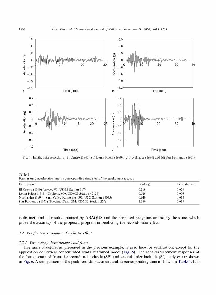
A computer program PAAP-Dyna is developed based on the above-mentioned formulation to predictvibration behavior of three-dimensional framed structures as well as its nonlinear response under earth-quake loading. It is verified for validity using the results generated by ABAQUS program through threenumerical examples. Although the use of shell element of ABAQUS can lead to extremely accurate results,it is not applied here because it is too time-consuming for such a nonlinear dynamic analysis. Therefore, theB33 beam element with 13 numerical integration points (five points in web, five in each flange) of ABAQUSis used to model framed structures herein. Four earthquake records of the El-Centro 1940, the Loma Prieta1989, the Northridge 1994, and the San Fernando 1971, as presented in Fig. 1, are used as ground motioninput data. Their peak ground accelerations and time steps are listed in Table 1. For each problem, the sta-tic load due to the weight of the mass and dead loading (if any) is applied first to the structure by a staticanalysis, and then the earthquake loading is applied by a dynamic time-history analysis. The mass- andstiffness-proportional damping factors are chosen based on first two modes of frame so that the equivalentviscous damping ratio is equal to 5%.

3.1. Two-storey three-dimensional frame for second-order effect verification

Fig. 2 shows the geometric and material properties of a two-storey three-dimensional frame with masseslumped at the framed nodes. The geometry of this frame is symmetric, but the mass distribution is not. Thevertical concentrated loads applied at all framed nodes are chosen to be very large in order to show thesecond-order effect clearly. In numerical modeling, each framed element is divided into two equal elements.

After performing the vibration analysis, first two natural periods along the applied earthquake directionand corresponding mode shapes of the frame are obtained and compared in Table 2 and Fig. 3. It can beseen that a strong agreement of dynamic properties of the study frame generated by ABAQUS and pro-posed programs is obtained.

The roof displacement responses of frame and a comparison of their peak values and correspondingtimes of the linear elastic (LE) and second-order elastic (SE) analyses are shown in Fig. 4 and Table 3.As can be observed from those, the difference of displacement response of LE and SE analyses in each case

-1.2

-0.9

-0.6

-0.3

0

0.3

0.6

0.9

0 10 20

Time (sec)

Acce

lera

tion

(g)

Acce

lera

tion

(g)

30

-1.2

-0.9

-0.6

-0.3

0

0.3

0.6

0.9

0 10 20 30

Time (sec)

40

-1.2

-0.9

-0.6

-0.3

0

0.3

0.6

0.9

0 5 10 15 20 25

Time (sec)

Acce

lera

tion

(g)

-1.2

-0.9

-0.6

-0.3

0

0.3

0.6

0.9

0 10 20 30

Time (sec)

Acce

lera

tion

(g)

40

a b

c d

Fig. 1. Earthquake records: (a) El Centro (1940); (b) Loma Prieta (1989); (c) Northridge (1994) and (d) San Fernando (1971).

Table 1Peak ground acceleration and its corresponding time step of the earthquake records

Earthquake PGA (g) Time step (s)

El Centro (1940) (Array, #9, USGS Station 117) 0.319 0.020Loma Prieta (1989) (Capitola, 000, CDMG Station 47125) 0.529 0.005Northridge (1994) (Simi Valley-Katherine, 090, USC Station 90055) 0.640 0.010San Fernando (1971) (Pacoima Dam, 254, CDMG Station 279) 1.160 0.010


is distinct, and all results obtained by ABAQUS and the proposed programs are nearly the same, whichprove the accuracy of the proposed program in predicting the second-order effect.

3.2. Verification examples of inelastic effect

3.2.1. Two-storey three-dimensional frame

The same structure, as presented in the previous example, is used here for verification, except for theapplication of vertical concentrated loads at framed nodes (Fig. 5). The roof displacement responses ofthe frame obtained from the second-order elastic (SE) and second-order inelastic (SI) analyses are shownin Fig. 6. A comparison of the peak roof displacement and its corresponding time is shown in Table 4. It is

-1.0 -0.5 0.0 0.5 1.0

1st mode

-1.0 -0.5 0.0 0.5 1.0

2nd mode

ABAQUSPAAP-Dyna

Fig. 3. Comparison of first two mode shapes along the applied earthquake direction of two-storey frame.

Fig. 2. Two-storey frame for second-order effect verification.

Table 2Comparison of first two natural periods along the applied earthquake direction of two-storey frame

Mode Period (s) Error (%)

ABAQUS PAAP-Dyna (proposed)

First 0.4340 0.4352 �0.28Second 0.1217 0.1220 �0.32


-60

-40

-20

0

20

40

60

0 10 20

Time (sec)

Dis

plac

emen

t (m

m)

30

ABAQUS (LE)PAAP-Dyna (LE)

-60

-40

-20

0

20

40

60

0 10 20

Time (sec)

Dis

plac

emen

t (m

m)

30

ABAQUS (SE)PAAP-Dyna (SE)

-80

-60

-40

-20

0

20

40

60

80

0 10 20 30

Time (sec)

Time (sec) Time (sec)

Time (sec) Time (sec)

Dis

plac

emen

t (m

m)

Dis

plac

emen

t (m

m)

Dis

plac

emen

t (m

m)

40


-80

-60

-40

-20

0

20

40

60

80

0 10 20 30t

Time (sec)

Dis

plac

emen

t (m

m)

40


-120

-90

-60

-30

0

30

60

90

120

0 5 10 15 20 25


-120

-90

-60

-30

0

30

60

90

120

0 5 10 15 20 25


-160

-120

-80

-40

0

40

80

120

160

0 10 20 30 40


-160

-120

-80

-40

0

40

80

120

160

0 10 20 30

Dis

plac

emen

t (m

m)

Dis

plac

emen

t (m

m)

40


a

b

c

d

Fig. 4. Roof displacements of two-storey frame for second effect verification: (a) El Centro earthquake; (b) Loma Prieta earthquake;(c) Northridge earthquake and (d) San Fernando earthquake.


Table 3Comparison of peak roof displacement and its corresponding time of two-storey frame for second-order effect verification

Eq. type Min/max Analysis type ABAQUS PAAP-Dyna (proposed) Disp. Error (%)

Disp. (mm) Time (s) Disp. (mm) Time (s)

El Centro Max LE 36.42 2.520 35.74 2.520 1.87SE 49.32 2.120 48.21 2.100 2.25

Min LE �44.22 2.740 �42.98 2.740 2.80SE �58.25 2.340 �57.86 2.340 0.67

Loma Prieta Max LE 77.41 6.950 75.07 6.940 3.02SE 52.14 7.565 51.90 7.555 0.46

Min LE �73.13 6.755 �71.39 6.745 2.38SE �49.10 6.385 �48.17 6.380 1.89

Northridge Max LE 89.63 5.010 86.38 5.010 3.63SE 111.45 7.600 110.71 7.600 0.66

Min LE �94.73 5.230 �92.14 5.230 2.73SE �114.57 7.840 �112.65 7.840 1.68

San Fernando Max LE 132.92 8.600 129.38 8.590 2.66SE 156.29 8.620 154.56 8.610 1.11

Min LE �133.89 8.810 �130.89 8.800 2.24SE �146.71 8.860 �145.24 8.840 1.00

Fig. 5. Two-storey frame for inelastic effect verification.


observed that the ABAQUS and proposed programs give nearly identical results in all cases, including theslight permanent shifts in displacement due to inelastic behavior for SI analysis cases under Loma Prieta,Northridge, and San Fernando earthquakes. As is evident from the figure, the difference in displacementresponse of SE and SI analyses in these cases is relatively clear. For the case of El Centro earthquake havingsmallest PGA, it is noted that the displacement responses in SE and SI cases are almost identical, becausethe behavior of the framed structure is almost in elastic range in this case.

-50

-40

-30

-20

-10

0

10

20

30

40

50

0 10 20

Time (sec)

Time (sec)

30

ABAQUS (SI)PAAP-Dyna (SE)

-50

-40

-30

-20

-10

0

10

20

30

40

50

0 10 20

Time (sec)

30

ABAQUS (SI)PAAP-Dyna (SI)

-80

-60

-40

-20

0

20

40

60

80

0 10 20 30 40


-80

-60

-40

-20

0

20

40

60

80

0 10 20 30

Time (sec)

40


-100

-80

-60

-40

-20

0

20

40

60

80

100

0 5 10 15 20 25

Time (sec)


-100

-80

-60

-40

-20

0

20

40

60

80

100

0 5 10 15 20 25


Dis

plac

emen

t (m

m)

Dis

plac

emen

t (m

m)

Dis

plac

emen

t (m

m)

Dis

plac

emen

t (m

m)

Dis

plac

emen

t (m

m)

Dis

plac

emen

t (m

m)

-140

-100

-60

-20

20

60

100

140

0 10 20 30

Time (sec)

40


-140

-100

-60

-20

20

60

100

140

0 10 20 30

Time (sec)

Time (sec)

40


Dis

plac

emen

t (m

m)

Dis

plac

emen

t (m

m)

a

b

c

d

Fig. 6. Roof displacements of two-storey frame for inelastic effect verification: (a) El Centro earthquake; (b) Loma Prieta earthquake;(c) Northridge earthquake and (d) San Fernando earthquake.


Table 4Comparison of peak roof displacement and its corresponding time of two-storey frame for inelastic effect verification

Eq. type Min/max Analysis type ABAQUS PAAP-Dyna (proposed) Disp. Error (%)

Disp. (mm) Time (s) Disp. (mm) Time (s)

El Centro Max SE 36.95 2.520 35.69 2.520 3.40SI 36.95 2.520 35.69 2.520 3.40

Min SE �44.67 2.740 �43.02 2.740 3.68SI �44.67 2.740 �43.02 2.740 3.68

Loma Prieta Max SE 75.62 6.950 74.97 6.940 0.86SI 71.49 6.950 69.87 6.940 2.28

Min SE �72.46 6.755 �71.40 6.745 1.74SI �70.71 6.755 �68.46 6.750 3.18

Northridge Max SE 87.38 5.010 86.24 5.010 1.28SI 79.98 5.010 77.77 5.010 2.77

Min SE �93.07 5.240 �92.14 5.230 1.00SI �78.22 4.400 �76.60 4.400 2.07

San Fernando Max SE 130.88 8.600 129.50 8.590 1.05SI 95.21 8.620 93.41 8.610 1.90

Min SE �131.46 8.820 �131.08 8.800 0.29SI �103.89 8.380 �103.84 8.370 0.04


3.2.2. Four-storey three-dimensional frame

This four-storey, two by two bay steel frame was presented by Campbell (1994). The framed geometryand members are kept to be same to the original frame, but the in-plane rigid slabs are neglected in mod-eling. Besides, because the original masses were too small, they are changed into bigger ones to be morerealistic and to be capable of showing inelastic behavior clearly under earthquakes. The geometry, massdistribution, and material properties of the modified frame are shown in Fig. 7. Each member of the frameis only modeled by one element in numerical modeling.

A comparison of first three natural periods along the applied earthquake direction and their corre-sponding mode shapes of the four-storey frame obtained by vibration analysis of ABAQUS and theproposed programs are shown in Table 5 and Fig. 8. It can be seen that a very good correlation isfound.

The roof displacement responses along X-axis of node A of the frame obtained by ABAQUS and pro-posed programs are shown in Fig. 9 for four different earthquakes. Their peak displacements and corre-sponding times are compared in Table 6. It is observed that except for the similar response in the casesof the frame subjected to the El Centro earthquake with the smallest PGA, the difference of displacementresponse of SE and SI analyses in the other cases is clear, and the obtained results correlate very well,including the permanent drifts of displacement in SI analysis cases. As in the previous example, this onealso indicates that the proposed program is able to accurately predict displacements, which is an importantindex for a performance-based seismic design.

The locations of plastic hinges and their corresponding times at the most severe yielding state of thisstudy frame subjected to Northridge and San Fernando earthquakes are shown in Fig. 10. It can be seenthat the results obtained by ABAQUS and PAAP-Dyna are similar.

With using Intel Pentium IV 3.2 GHz, 2 GB RAM computer, the computational times of the ABAQUSand PAAP-Dyna programs for four-storey frame subjected to Loma-Prieta earthquake, which is the prob-lem having the longest analysis time among four cases, are 12 h and 5 min, respectively. This result provesthe high computational efficiency of the proposed computer program.

Fig. 7. Four-storey frame.

Table 5Comparison of first three natural periods along the applied earthquake direction of four-storey frame (X direction)

Mode Period (s) Error (%)

ABAQUS PAAP-Dyna (proposed)

First 1.1764 1.1746 0.15Second 0.4077 0.4029 1.18Third 0.1714 0.1707 0.41

-1.0 -0.5 0.0 0.5 1.01st mode

-1.0 -0.5 0.0 0.5 1.0

2nd mode

ABAQUSPAAP-Dyna

-1.0 -0.5 0.0 0.5 1.0

3rd mode

Fig. 8. Comparison of first three mode shapes along the applied earthquake direction of four-storey frame (X-direction).


a

b

c

d

Fig. 9. Roof displacements at node A of four-storey frame: (a) El Centro earthquake; (b) Loma Prieta earthquake; (c) Northridgeearthquake and (d) San Fernando earthquake.


Table 6Comparison of peak roof displacement at node A and its corresponding time of four-storey frame

Eq. type Min/max Analysis type ABAQUS PAAP-Dyna (proposed) Disp. error (%)

Disp. (in) Time (s) Disp. (in) Time (s)

El Centro Max SE 5.013 3.520 5.042 3.500 �0.58SI 4.901 3.520 4.847 4.520 1.11

Min SE �4.538 2.980 �4.458 2.960 1.75SI �4.575 2.980 �4.612 2.960 �0.81

Loma Prieta Max SE 8.880 9.355 8.531 9.34 3.93SI 7.845 14.39 7.617 14.39 2.91

Min SE �8.791 9.960 �8.535 9.960 2.91SI �6.846 8.755 �6.490 8.750 5.21

Northridge Max SE 9.235 5.120 8.838 5.110 4.30SI 5.436 5.140 5.227 5.140 3.85

Min SE �8.863 5.520 �9.064 5.510 �2.27SI �5.694 5.500 �5.475 5.500 3.85

San Fernando Max SE 11.414 3.660 11.027 3.630 3.39SI 12.149 3.720 11.744 3.720 3.33

Min SE �12.242 4.230 �12.045 4.200 1.61SI �6.911 3.190 �6.804 3.170 1.54

Fig. 10. Plastic hinge formation at the most severe yielding state of four-storey frame: (a) Northridge earthquake ABAQUS: t = 5.50 s;PAAP-Dyna, t = 5.50 s and (b) San Fernando earthquake: ABAQUS: t = 3.72 s; PAAP-Dyna, t = 3.71 s.


4. Conclusions

A simple and effective numerical procedure for the nonlinear dynamic time-history analysis of the three-dimensional steel frames considering both geometric and material nonlinearities has been presented. Thecomputer program developed for this research is verified for accuracy and computational efficiency through


three numerical examples with four different earthquake loadings. It is also capable of accurately predictingnatural periods and vibration mode shapes of framed structures. The good results obtained in a short anal-ysis time prove that this computer program can effectively be used for office design in predicting nonlinearbehavior of steel framed structures subjected to static and dynamic load instead of using the time-consum-ing and costly commercial structural software.

Acknowledgement

The work presented in this paper was supported by funds of National Research Laboratory Program(Grant No. M1-0204-00-0143-04-J00-00-083-10) from Ministry of Science and Technology in Korea.Authors wish to appreciate this financial support.

References

Al-Bermani, F.G.A., Zhu, K., 1996. Nonlinear elastoplastic analysis of spatial structures under dynamic loading using kinematichardening models. Engineering Structures 18 (8), 568–576.

Campbell, S.D., 1994. Nonlinear elements for three dimensional frame analysis. Ph.D. Thesis, University of California at Berkeley,CA.

Chan, S.L., 1996. Large deflection dynamic analysis of space frames. Computer and Structures 58 (2), 381–387.Chen, W.F., Lui, E.M., 1987. Structural Stability: Theory and Implementation. Elsevier, New York.Chi, W.M., El-Tawil, S., Deierlein, G.G., Abel, J.F., 1998. Inelastic analyses of a 17-storey steel framed building damaged during

Northridge. Engineering Structures 20 (4–6), 481–495.Chopra, A.K., 2001. Dynamics of Structures: Theory and Applications to Earthquake Engineering. Prentice-Hall, New Jersey.El-Tawil, S., Deierlein, G.G., 2001. Nonlinear analysis of mixed steel–concrete frames, Parts I and II. Journal of Structural

Engineering 127 (6), 647–665.Izzuddin, B.A., Smith, D.L., 1996. Large-displacement analysis of elastoplastic thin-walled frames, part I and II. Journal of Structural

Engineering 122 (8), 905–925.Jiang, X.M., Chen, H., Liew, J.Y.R., 2002. Spread-of-plasticity analysis of three-dimensional steel frames. Journal of Constructional

Steel Research 58 (2), 193–212.Kim, S.E., Lee, J., Park, J.S., 2002. 3-D second-order plastic-hinge analysis accounting for lateral torsional buckling. International

Journal of Solids and Structures 39 (8), 2109–2128.Kim, S.E., Lee, J., Park, J.S., 2003. 3-D second-order plastic-hinge analysis accounting for local buckling. Engineering Structures 25

(1), 81–90.Kim, S.E., Park, M.H., Choi, S.H., 2001. Direct design of three-dimensional frames using practical advanced analysis. Engineering

Structures 23 (11), 1491–1502.Liew, J.Y.R., Chen, H., Shanmugam, N.E., Chen, W.F., 2000. Improved nonlinear plastic hinge analysis of space frame structures.

Engineering Structures 22 (10), 1324–1338.McGuire, W., Gallagher, R.H., Ziemian, R.D., 2000. Matrix Structural Analysis. John Wiley & Son, Inc., New York.McKenna, F., Fenves, G.L., et al., 2005. Open system for earthquake engineering simulation (OpenSees). Available from:

<http://opensees.berkeley.edu>. Pacific Earthquake Engineering Research Center, University of California, Berkeley.Porter, F.L., Powell, G.H., 1971. Static and dynamic analysis of inelastic frame structures. Report No. EERC 71-3, University of

California, Berkeley.Teh, L.H., Clark, M.J., 1999. Plastic-zone analysis of 3D steel frames using beam elements. Journal of Structural Engineering 125 (11),

1328–1337.

http://opensees.berkeley.edu

Second-order inelastic dynamic analysis of 3-D steel...

Documents

Transcript of Second-order inelastic dynamic analysis of 3-D steel...