Sebastian Eggert- Impurity Effects in Antiferromagnetic Quantum Spin-1/2 Chains
132
IMPURITY EFFECTS IN ANTIFERROMAGNETIC QUANTUM SPIN-1/2 CHAINS By Sebastian Eggert M. Sc. (Physics) University of Wyoming, 1990 a thesis submitted in partial fulfillment of the requirements for the degree of Doctor of Philosophy in the faculty of gradua te studies dep ar tment of phys ics We accept this thesis as conforming to the required standard ....................................................... ....................................................... ....................................................... ....................................................... the university of british columbia 1994 c Sebastian Eggert, 2003
Transcript of Sebastian Eggert- Impurity Effects in Antiferromagnetic Quantum Spin-1/2 Chains

8/3/2019 Sebastian Eggert- Impurity Effects in Antiferromagnetic Quantum Spin-1/2 Chains
http://slidepdf.com/reader/full/sebastian-eggert-impurity-effects-in-antiferromagnetic-quantum-spin-12-chains 1/132
IMPURITY EFFECTS IN ANTIFERROMAGNETIC QUANTUM SPIN-1/2 CHAINS
By
Sebastian Eggert
M. Sc. (Physics) University of Wyoming, 1990
a thesis submitted in partial fulfillment of
the requirements for the degree of
Doctor of Philosophy
in
the faculty of graduate studies
department of physics
We accept this thesis as conforming
to the required standard
. . . . . . . . . . . . . . . . . . . . . . . . . . . . . . . . . . . . . . . . . . . . . . . . . . . . . . .
. . . . . . . . . . . . . . . . . . . . . . . . . . . . . . . . . . . . . . . . . . . . . . . . . . . . . . .
. . . . . . . . . . . . . . . . . . . . . . . . . . . . . . . . . . . . . . . . . . . . . . . . . . . . . . .
. . . . . . . . . . . . . . . . . . . . . . . . . . . . . . . . . . . . . . . . . . . . . . . . . . . . . . .
the university of british columbia
1994
c Sebastian Eggert, 2003
8/3/2019 Sebastian Eggert- Impurity Effects in Antiferromagnetic Quantum Spin-1/2 Chains
http://slidepdf.com/reader/full/sebastian-eggert-impurity-effects-in-antiferromagnetic-quantum-spin-12-chains 2/132
Abstract
We calculate the effects of a single impurity in antiferromagnetic quantum spin-1/2 chains
with the help of one-dimensional quantum field theory and renormalization group tech-
niques in the low temperature limit. We are able to present numerical evidence from ex-
act diagonalization, numerical Bethe ansatz, and quantum Monte Carlo methods, which
support our findings. Special emphasis has been put on impurity effects on the local
susceptibility in the chain, because of the experimental relevance of this quantity. We
propose a muon spin resonance experiment on quasi one-dimensional spin compounds,
which may show some of the impurity effects.
ii

8/3/2019 Sebastian Eggert- Impurity Effects in Antiferromagnetic Quantum Spin-1/2 Chains
http://slidepdf.com/reader/full/sebastian-eggert-impurity-effects-in-antiferromagnetic-quantum-spin-12-chains 3/132
Table of Contents
Abstract ii
Table of Contents iii
List of Tables vi
List of Figures vii
Acknowledgements xv
1 Introduction 1
1.1 The Hamiltonian . . . . . . . . . . . . . . . . . . . . . . . . . . . . . . . 1
1.2 Impurities . . . . . . . . . . . . . . . . . . . . . . . . . . . . . . . . . . . 2
1.3 Experimental Relevance . . . . . . . . . . . . . . . . . . . . . . . . . . . 5
1.4 Outline . . . . . . . . . . . . . . . . . . . . . . . . . . . . . . . . . . . . . 6
2 Theoretical Background 8
2.1 From the Lattice Model to the Quantum Field Theory . . . . . . . . . . 8
2.2 Symmetries . . . . . . . . . . . . . . . . . . . . . . . . . . . . . . . . . . 12
2.3 Correlation Functions . . . . . . . . . . . . . . . . . . . . . . . . . . . . . 13
3 Scaling and Finite Size Effects 15
3.1 Boundary Conditions . . . . . . . . . . . . . . . . . . . . . . . . . . . . . 15
3.1.1 Periodic boundary conditions . . . . . . . . . . . . . . . . . . . . 153.1.2 Open boundary conditions . . . . . . . . . . . . . . . . . . . . . . 16
iii

8/3/2019 Sebastian Eggert- Impurity Effects in Antiferromagnetic Quantum Spin-1/2 Chains
http://slidepdf.com/reader/full/sebastian-eggert-impurity-effects-in-antiferromagnetic-quantum-spin-12-chains 4/132
3.2 Scaling and Irrelevant Operators . . . . . . . . . . . . . . . . . . . . . . . 18
3.3 Finite-size Spectrum . . . . . . . . . . . . . . . . . . . . . . . . . . . . . 22
3.3.1 Periodic boundary conditions . . . . . . . . . . . . . . . . . . . . 22
3.3.2 Open boundary conditions . . . . . . . . . . . . . . . . . . . . . . 25
4 Impurities 31
4.1 One Perturbed Link . . . . . . . . . . . . . . . . . . . . . . . . . . . . . 31
4.2 Two Perturbed Links . . . . . . . . . . . . . . . . . . . . . . . . . . . . . 36
4.3 Relation to Other Problems . . . . . . . . . . . . . . . . . . . . . . . . . 38
5 Susceptibilities 43
5.1 Periodic Chain Susceptibility . . . . . . . . . . . . . . . . . . . . . . . . . 44
5.1.1 Contributions from the leading irrelevant operator . . . . . . . . . 45
5.2 Open Chain Susceptibility . . . . . . . . . . . . . . . . . . . . . . . . . . 51
5.2.1 Contributions from the boundary condition . . . . . . . . . . . . . 52
5.2.2 Contributions from the leading irrelevant boundary operator . . . 56
5.3 Susceptibility Contributions from Perturbations . . . . . . . . . . . . . . 58
5.3.1 Two perturbed links . . . . . . . . . . . . . . . . . . . . . . . . . 61
5.3.2 One perturbed link . . . . . . . . . . . . . . . . . . . . . . . . . . 63
5.4 A Muon Spin Resonance Experiment . . . . . . . . . . . . . . . . . . . . 65
5.4.1 Experimental Setup . . . . . . . . . . . . . . . . . . . . . . . . . . 65
5.4.2 Field Theory Analysis . . . . . . . . . . . . . . . . . . . . . . . . 69
6 Monte Carlo Results 71
6.1 Impurity Susceptibility Effects . . . . . . . . . . . . . . . . . . . . . . . . 71
6.1.1 One weak link . . . . . . . . . . . . . . . . . . . . . . . . . . . . . 72
6.1.2 Two weak links . . . . . . . . . . . . . . . . . . . . . . . . . . . . 75
iv
8/3/2019 Sebastian Eggert- Impurity Effects in Antiferromagnetic Quantum Spin-1/2 Chains
http://slidepdf.com/reader/full/sebastian-eggert-impurity-effects-in-antiferromagnetic-quantum-spin-12-chains 5/132
6.1.3 Alternating Parts . . . . . . . . . . . . . . . . . . . . . . . . . . . 76
6.2 Muon Knight Shift . . . . . . . . . . . . . . . . . . . . . . . . . . . . . . 80
6.2.1 One perturbed link . . . . . . . . . . . . . . . . . . . . . . . . . . 84
6.2.2 Two perturbed links . . . . . . . . . . . . . . . . . . . . . . . . . 92
6.3 Conclusions . . . . . . . . . . . . . . . . . . . . . . . . . . . . . . . . . . 96
A Field Theory Formulas 106
B Exact Diagonalization Algorithm 109
C Monte Carlo Algorithm 111
Bibliography 115
v

8/3/2019 Sebastian Eggert- Impurity Effects in Antiferromagnetic Quantum Spin-1/2 Chains
http://slidepdf.com/reader/full/sebastian-eggert-impurity-effects-in-antiferromagnetic-quantum-spin-12-chains 6/132
List of Tables
3.1 Low energy spectrum for periodic boundary conditions. Relative parity
and total spin are given. . . . . . . . . . . . . . . . . . . . . . . . . . . . 24
3.2 Low energy spectrum for open boundary conditions. Relative parity and
total spin are given. . . . . . . . . . . . . . . . . . . . . . . . . . . . . . . 28
vi

8/3/2019 Sebastian Eggert- Impurity Effects in Antiferromagnetic Quantum Spin-1/2 Chains
http://slidepdf.com/reader/full/sebastian-eggert-impurity-effects-in-antiferromagnetic-quantum-spin-12-chains 7/132
List of Figures
1.1 An impurity breaks conformal invariance and renormalizes to a boundary
condition. . . . . . . . . . . . . . . . . . . . . . . . . . . . . . . . . . . . 3
1.2 An analytic continuation of left movers in terms of right movers to the
negative half axis effectively removes the boundary and restores conformal
invariance. . . . . . . . . . . . . . . . . . . . . . . . . . . . . . . . . . . . 4
3.3 Numerical low energy spectrum for periodic, even length l = 20 spin chain.
The integer values El/πv of the numerically accessible states agree with
the theoretical predictions. The velocity vπ = 3.69 was used (see figure 3.5). 25
3.4 Numerical low energy spectrum for periodic, odd length l = 19 spin chain
(vπ = 3.69). . . . . . . . . . . . . . . . . . . . . . . . . . . . . . . . . . . 26
3.5 Renormalization group flow towards the asymptotic spectrum of the peri-
odic chain. The lowest excitation gap 0+, 1− is fitted to l E = a + b/l2 for
even lengths (a = 3.69, b = 3.94). . . . . . . . . . . . . . . . . . . . . . . 27
3.6 Numerical low energy spectrum for the open, even length l = 20 spin chain
(vπ = 3.42). . . . . . . . . . . . . . . . . . . . . . . . . . . . . . . . . . . 29
3.7 Numerical low energy spectrum for the open, odd length l = 19 spin chain
(vπ = 3.42). . . . . . . . . . . . . . . . . . . . . . . . . . . . . . . . . . . 29
3.8 Renormalization group flow towards the asymptotic spectrum for the open
chain. The lowest excitation gap E (l/πv) is fitted to l E = a + b/l for both
even and odd length chains (a = 3.65, b =−
4.6). . . . . . . . . . . . . . 30
4.9 A quantum spin chain with one altered link. . . . . . . . . . . . . . . . . 32
vii

8/3/2019 Sebastian Eggert- Impurity Effects in Antiferromagnetic Quantum Spin-1/2 Chains
http://slidepdf.com/reader/full/sebastian-eggert-impurity-effects-in-antiferromagnetic-quantum-spin-12-chains 8/132
4.10 Flow away from the periodic chain fixed point due to one altered link for
an odd length chain with 7 ≤ l ≤ 23. The lowest excitation gap 12
+, 1
2
−is
fitted to lE = a l1/2, which is the predicted scaling. . . . . . . . . . . . . 35
4.11 Renormalization group flow towards the open chain fixed point due to one
weak link for an odd length chain with 7 ≤ l ≤ 23. The corrections to the
lowest excitation gap 12
+, 1
2
−is fitted to l∆E = a/l + b/l2, exhibiting the
predicted 1/l scaling up to higher order. . . . . . . . . . . . . . . . . . . 36
4.12 A quantum spin chain with two altered links. . . . . . . . . . . . . . . . 37
4.13 Flow towards the periodic chain fixed point for two altered antiferromag-
netic links. The 12
+, 12
−gap is fitted to lE = a/l1/2, which is the predicted
scaling. . . . . . . . . . . . . . . . . . . . . . . . . . . . . . . . . . . . . . 38
4.14 Flow away from the open chain fixed point for two weak antiferromagnetic
links. Corrections to the 12
+, 12
−gap are fitted to ∆E/E = (a+b/l +c ln l),
demonstrating relevant logarithmic scaling (ac > 0). The dotted line is
the best fit for c = 0. . . . . . . . . . . . . . . . . . . . . . . . . . . . . 39
4.15 Flow towards the open chain fixed point for two weak ferromagnetic links.
Corrections to the 12
+, 32
−gap are fitted to ∆E/E = (a + b/l + c ln l),
demonstrating irrelevant logarithmic scaling (ac < 0). The dotted line is
the best fit for c = 0. . . . . . . . . . . . . . . . . . . . . . . . . . . . . . 39
4.16 The equivalent spin chain model to the two impurity Kondo problem. . . 41
5.17 χ(T ) from the Bethe ansatz. χ(0) = 1/Jπ2 is taken from equation (5.67). 48
5.18 Field theory [equation (5.76), T 0 ≈ 7.7J ] versus Bethe ansatz results for
χ(T ) at low temperature. . . . . . . . . . . . . . . . . . . . . . . . . . . . 49
viii

8/3/2019 Sebastian Eggert- Impurity Effects in Antiferromagnetic Quantum Spin-1/2 Chains
http://slidepdf.com/reader/full/sebastian-eggert-impurity-effects-in-antiferromagnetic-quantum-spin-12-chains 9/132
5.19 Estimates for the effective coupling g from lowest order perturbation the-
ory correction to the finite-size energy of ground-state, first excited triplet
state, first excited singlet state[19] and to the susceptibility, using l ↔ v/T .
The renormalization group prediction of equation (5.75) is also shown. . . 50
5.20 The open ends of the broken chain are expected to be more susceptible. . 52
5.21 The local susceptibility near open ends from Monte Carlo simulations for
β = 15/J . . . . . . . . . . . . . . . . . . . . . . . . . . . . . . . . . . . . 54
5.22 The uniform and alternating parts of the local susceptibility near open ends 55
5.23 Renormalization group analysis of the cross-over from an unstable to a
stable fixed point as the temperature is lowered. . . . . . . . . . . . . . . 59
5.24 Schematic Muon Spin Resonance setup: One Muon at a time enters through
the thin timer and stops inside the sample where its spin precesses. Decay
positrons are detected in the two counters. . . . . . . . . . . . . . . . . . 66
5.25 The location of the muon relative to the chain for the link parity symmetric
case. . . . . . . . . . . . . . . . . . . . . . . . . . . . . . . . . . . . . . . 67
6.26 The open chain impurity susceptibility as a function of temperature. The
solid line is only drawn for visual guidance and does not necessarily reflect
an accurate estimate. . . . . . . . . . . . . . . . . . . . . . . . . . . . . . 73
6.27 The impurity susceptibility for a small coupling J across the open ends
as a function of temperature. . . . . . . . . . . . . . . . . . . . . . . . . 74
6.28 The impurity susceptibility for a small perturbation δJ of one link in the
chain as a function of temperature. The solid lines are only drawn for
visual guidance and do not necessarily reflect an accurate estimate. . . . 75
6.29 The impurity susceptibility for a small perturbation δJ of two links in the
chain as a function of temperature. . . . . . . . . . . . . . . . . . . . . . 77
ix

8/3/2019 Sebastian Eggert- Impurity Effects in Antiferromagnetic Quantum Spin-1/2 Chains
http://slidepdf.com/reader/full/sebastian-eggert-impurity-effects-in-antiferromagnetic-quantum-spin-12-chains 10/132
6.30 The local susceptibility correction of the central spin closest to the impu-
rity for a small perturbation δJ on two links in the chain as a function of
temperature. . . . . . . . . . . . . . . . . . . . . . . . . . . . . . . . . . . 77
6.31 The impurity susceptibility for a small coupling J of the open ends to an
impurity spin as a function of temperature. . . . . . . . . . . . . . . . . 78
6.32 The local susceptibility of an impurity spin coupled with a small pertur-
bation J to the open ends of the chain as a function of temperature. . . 78
6.33 The local susceptibility as a function of distance from a weakened link
J = 0.75J at T = J/15. . . . . . . . . . . . . . . . . . . . . . . . . . . . 79
6.34 The alternating part of the local susceptibility as a function of distance
from the weakly coupled link J across the open ends at T = J/15. . . . . 80
6.35 The local susceptibility as a function of distance with the open ends cou-
pled with J = 0.1J to an impurity spin at the first site at T = J/15. . . 81
6.36 The local susceptibility as a function of distance with the open ends cou-
pled with J = 0.25J to an impurity spin at the first site at T = J/15. . . 81
6.37 The local susceptibility as a function of distance with the open ends cou-
pled with J = 0.5J to an impurity spin at the first site T = J/15. . . . . 82
6.38 The local susceptibility as a function of distance from two slightly weak-
ened links J = 0.75J at T = J/15. . . . . . . . . . . . . . . . . . . . . . 82
6.39 The effective normalized susceptibility in a powdered sample for small
perturbations on one link and d⊥ = 0.5 as a function of temperature. . . 84
6.40 The effective normalized susceptibility in a powdered sample for small
perturbations on one link and d⊥ = 1 as a function of temperature. . . . 85
6.41 The effective normalized susceptibility in a powdered sample for one strength-
ened link and d⊥ = 0.5 as a function of temperature. . . . . . . . . . . . 86
x

8/3/2019 Sebastian Eggert- Impurity Effects in Antiferromagnetic Quantum Spin-1/2 Chains
http://slidepdf.com/reader/full/sebastian-eggert-impurity-effects-in-antiferromagnetic-quantum-spin-12-chains 11/132
6.42 The effective normalized susceptibility in a powdered sample for one strength-
ened link and d⊥ = 1 as a function of temperature. . . . . . . . . . . . . 87
6.43 The effective normalized susceptibility in a powdered sample for strong
perturbations on one link and d⊥ = 0.5 as a function of temperature. . . 87
6.44 The effective normalized susceptibility in a powdered sample for strong
perturbations on one link and d⊥ = 1 as a function of temperature. . . . 88
6.45 The effective normalized susceptibility for an applied field perpendicular
to the chain, small perturbations on one link and d⊥ = 0.5 as a function
of temperature. . . . . . . . . . . . . . . . . . . . . . . . . . . . . . . . . 89
6.46 The effective normalized susceptibility for an applied field perpendicular
to the chain, small perturbations on one link and d⊥ = 1 as a function of
temperature. . . . . . . . . . . . . . . . . . . . . . . . . . . . . . . . . . . 89
6.47 The effective normalized susceptibility for an applied field perpendicular to
the chain, one strengthened link and d⊥ = 0.5 as a function of temperature. 90
6.48 The effective normalized susceptibility for an applied field perpendicular
to the chain, one strengthened link and d⊥ = 1 as a function of temperature. 90
6.49 The effective normalized susceptibility for an applied field perpendicular
to the chain, strong perturbations on one link and d⊥
= 0.5 as a function
of temperature. . . . . . . . . . . . . . . . . . . . . . . . . . . . . . . . . 91
6.50 The effective normalized susceptibility for an applied field perpendicular
to the chain, strong perturbations on one link and d⊥ = 1 as a function of
temperature. . . . . . . . . . . . . . . . . . . . . . . . . . . . . . . . . . . 91
6.51 The effective normalized susceptibility for an applied field parallel to the
chain, small perturbations on one link and d⊥ = 0.5 as a function of
temperature. . . . . . . . . . . . . . . . . . . . . . . . . . . . . . . . . . . 92
xi

8/3/2019 Sebastian Eggert- Impurity Effects in Antiferromagnetic Quantum Spin-1/2 Chains
http://slidepdf.com/reader/full/sebastian-eggert-impurity-effects-in-antiferromagnetic-quantum-spin-12-chains 12/132
6.52 The effective normalized susceptibility for an applied field parallel to the
chain, one strengthened link and d⊥ = 0.5 as a function of temperature. . 93
6.53 The effective normalized susceptibility for an applied field parallel to the
chain, strong perturbations on one link and d⊥ = 0.5 as a function of
temperature. . . . . . . . . . . . . . . . . . . . . . . . . . . . . . . . . . . 93
6.54 The effective normalized susceptibility for an applied field parallel to the
chain, small perturbations on one link and d⊥ = 1 as a function of tem-
perature. . . . . . . . . . . . . . . . . . . . . . . . . . . . . . . . . . . . . 94
6.55 The effective normalized susceptibility for an applied field parallel to the
chain, one strengthened link and d⊥ = 1 as a function of temperature. . . 94
6.56 The effective normalized susceptibility for an applied field parallel to the
chain, strong perturbations on one link and d⊥ = 1 as a function of tem-
perature. . . . . . . . . . . . . . . . . . . . . . . . . . . . . . . . . . . . . 95
6.57 The effective normalized susceptibility in a powdered sample for small
perturbations on two links and d⊥ = 0.5 as a function of temperature. . . 96
6.58 The effective normalized susceptibility in a powdered sample for small
perturbations on two links and d⊥ = 1 as a function of temperature. . . . 97
6.59 The effective normalized susceptibility in a powdered sample for strong
perturbations on two links and d⊥ = 0.5 as a function of temperature. . . 97
6.60 The effective normalized susceptibility in a powdered sample for strong
perturbations on two links and d⊥ = 1 as a function of temperature. . . . 98
6.61 The effective normalized susceptibility in a powdered sample for two strength-
ened links and d⊥ = 0.5 as a function of temperature. . . . . . . . . . . . 98
6.62 The effective normalized susceptibility in a powdered sample for two strength-
ened links and d⊥ = 1 as a function of temperature. . . . . . . . . . . . . 99
xii

8/3/2019 Sebastian Eggert- Impurity Effects in Antiferromagnetic Quantum Spin-1/2 Chains
http://slidepdf.com/reader/full/sebastian-eggert-impurity-effects-in-antiferromagnetic-quantum-spin-12-chains 13/132
6.63 The effective normalized susceptibility for an applied field perpendicular
to the chain, small perturbations on two links and d⊥ = 0.5 as a function
of temperature. . . . . . . . . . . . . . . . . . . . . . . . . . . . . . . . . 99
6.64 The effective normalized susceptibility for an applied field perpendicular
to the chain, small perturbations on two links and d⊥ = 1 as a function of
temperature. . . . . . . . . . . . . . . . . . . . . . . . . . . . . . . . . . . 100
6.65 The effective normalized susceptibility for an applied field perpendicular to
the chain, two strengthened links and d⊥ = 0.5 as a function of temperature.100
6.66 The effective normalized susceptibility for an applied field perpendicular
to the chain, two strengthened links and d⊥ = 1 as a function of temperature.101
6.67 The effective normalized susceptibility for an applied field perpendicular
to the chain, strong perturbations on two links and d⊥ = 0.5 as a function
of temperature. . . . . . . . . . . . . . . . . . . . . . . . . . . . . . . . . 101
6.68 The effective normalized susceptibility for an applied field parallel to the
chain, small perturbations on two links and d⊥ = 0.5 as a function of
temperature. . . . . . . . . . . . . . . . . . . . . . . . . . . . . . . . . . . 102
6.69 The effective normalized susceptibility for an applied field parallel to the
chain, two strengthened links and d⊥
= 0.5 as a function of temperature. 102
6.70 The effective normalized susceptibility for an applied field parallel to the
chain, strong perturbations on two links and d⊥ = 0.5 as a function of
temperature. . . . . . . . . . . . . . . . . . . . . . . . . . . . . . . . . . . 103
6.71 The effective normalized susceptibility for an applied field parallel to the
chain, small perturbations on two links and d⊥ = 1 as a function of tem-
perature. . . . . . . . . . . . . . . . . . . . . . . . . . . . . . . . . . . . . 103
6.72 The effective normalized susceptibility for an applied field parallel to the
chain, two strengthened links and d⊥ = 1 as a function of temperature. . 104
xiii

8/3/2019 Sebastian Eggert- Impurity Effects in Antiferromagnetic Quantum Spin-1/2 Chains
http://slidepdf.com/reader/full/sebastian-eggert-impurity-effects-in-antiferromagnetic-quantum-spin-12-chains 14/132
6.73 The effective normalized susceptibility for an applied field parallel to the
chain, small perturbations on two links and d⊥ = 1 as a function of tem-
perature. . . . . . . . . . . . . . . . . . . . . . . . . . . . . . . . . . . . . 104
xiv

8/3/2019 Sebastian Eggert- Impurity Effects in Antiferromagnetic Quantum Spin-1/2 Chains
http://slidepdf.com/reader/full/sebastian-eggert-impurity-effects-in-antiferromagnetic-quantum-spin-12-chains 15/132
Acknowledgements
I would like to give my special thanks to my advisor, Ian Affleck for his patience in
many long and helpful discussions. Without him and his extraordinary ability to pass
on his vast knowledge this thesis would not have been possible. I am also very grateful
for interesting discussions with Eugene Wong, Rob Kiefl, Bill Buyers, and Philip Stamp
which were helpful in preparing this thesis. Special thanks also go to a number of people
in the physics department with whom I had the pleasure to interact with in the past
years: Junwu Gan, Arnold Sikkema, Jacob Sagi, Gordon Semenoff, Erik Sørensen, Birger
Birgerson, and Michel Gingras.
At this point I would also like to acknowledge some of my former advisors, mentors,
and teachers which made a special contribution in my course of studies: Herr Unger, EbsHilf, Alexander Rauh, Glen Rebka, Lee Schick, and Ramarao Inguva.
xv
8/3/2019 Sebastian Eggert- Impurity Effects in Antiferromagnetic Quantum Spin-1/2 Chains
http://slidepdf.com/reader/full/sebastian-eggert-impurity-effects-in-antiferromagnetic-quantum-spin-12-chains 16/132
Chapter 1
Introduction
Considerable attention has been focused on spin-1/2 chains since Bethe’s original work
more than 60 years ago[1]. The large interest in these relatively simple many-body quan-
tum mechanical systems is no surprise, since they exhibit many fascinating cooperative
phenomena which may be shared by more complex models. The Bethe ansatz has been
refined over the years[2], and thermodynamic quantities can be calculated exactly for a
wide parameter range[3]. With the advent of conformal field theory and more computing
power, we are now able to understand the model even on a more detailed level as pre-
sented in this thesis. Another goal of this thesis is to link this theoretical knowledge to
real experimental systems with special emphasis on impurity effects.
1.1 The Hamiltonian
We can model the magnetic properties of insulators very well by describing the exchange
coupling between orbital spins in terms of an anisotropic Heisenberg coupling. It is
possible to have quasi one-dimensional spin systems, in which the spins form “chains”
along one crystal axis in the sense that the exchange coupling is much stronger between
neighboring spins within the chain compared to the coupling J ⊥ between spins of dif-
ferent chains. If we neglect this interchain coupling we can describe the model by the
Hamiltonian
H =
l−1i=1
[J
2 (S +i S −i+1 + S −i S
+i+1) + J z S
zi S
zi+1], (1.1)
1

8/3/2019 Sebastian Eggert- Impurity Effects in Antiferromagnetic Quantum Spin-1/2 Chains
http://slidepdf.com/reader/full/sebastian-eggert-impurity-effects-in-antiferromagnetic-quantum-spin-12-chains 17/132
Chapter 1. Introduction 2
where S +i , S −i are the usual spin-1/2 raising and lowering operators at site i, l is the total
number of sites, and J is taken to be positive. We may choose open boundary conditions
where the ends at the 1st and lth site are free, or we may impose periodic boundary
conditions where the ends are coupled with the same coupling constants, J and J z.
Some materials are known to exist for spin-1/2 which exhibit this one-dimensional
behavior to various degrees (e.g. KCuF3[4] and CPC[5]). The ratio J/J ⊥ is a measure
of the one-dimensional properties of the material since three dimensional Neel ordering
will occur for low temperatures T < T N , T N ∝ J ⊥[6]. In some materials a spin-Peierls
transition to a dimer phase may occur instead if the phonon-spin coupling is strong.
Typically the exchange coupling J is of the order of 20 − 1000K , while the ordering
temperature T N is at least one order of magnitude smaller. Experimental results in
KCuF3[4] and CPC[5] are reported to agree well with the prediction of the Hamiltonian
in equation (1.1) at the isotropic point J ≈ J z. Both J and J ⊥ arise from an exchange
integral since the dipole-dipole interaction is only in the mK range. We also neglected
the spin-orbit coupling which is generally also much smaller than the exchange coupling.
The effect of a spin-orbit coupling can be described by a single-ion anisotropy of the form
(S z)2 in the Hamiltonian, which reduces to a trivial c-number for spin-1/2.
1.2 Impurities
The main goal of this thesis is to provide a good understanding of impurity effects in
spin-1/2 chains. The study of impurities has always been a large part of solid state
physics, because there are many cases where impurities produce very interesting effects
and may even dominate the behavior of the system. The best known examples may be
semiconductor doping, the Kondo effect, and high temperature superconductors.

8/3/2019 Sebastian Eggert- Impurity Effects in Antiferromagnetic Quantum Spin-1/2 Chains
http://slidepdf.com/reader/full/sebastian-eggert-impurity-effects-in-antiferromagnetic-quantum-spin-12-chains 18/132
Chapter 1. Introduction 3
xx=0
impurityboundary
bulk
τ
v/TK
Figure 1.1: An impurity breaks conformal invariance and renormalizes to a boundarycondition.
Recently, there has been an increased theoretical interest in quantum impurity prob-
lems which can be described by (1+1) dimensional conformal field theories. The resulting
theory of boundary critical phenomena proved to be very successful in treating a vari-
ety of problems[8], with the Kondo problem being probably the most famous. It turns
out that our model system can be regarded as one example of this technique, so it is
instructive to present the central ideas of this approach at this point (see also reference
[8]).
Let us start with some gapless, scale invariant system that can be described by a
conformally invariant field theory. We may introduce a local, time-independent pertur-
bation as shown in figure 1.1, which represents the impurity in the system and breaks the
conformal invariance. It also creates a new energy scale in the system, which depends on
the initial strength of the perturbation and on the scaling dimensions of the perturbing
operators in the field theory. This energy scale is defined as the temperature where we
expect a breakdown of perturbation theory, which is often called T K in analogy with the
Kondo effect. It is reasonable to assume that the system will still be described by the
conformal field theory far away from the impurity, i.e. outside a “boundary layer” which
is defined by the new energy scale in the system i.e. with width v/T K , where v is the

8/3/2019 Sebastian Eggert- Impurity Effects in Antiferromagnetic Quantum Spin-1/2 Chains
http://slidepdf.com/reader/full/sebastian-eggert-impurity-effects-in-antiferromagnetic-quantum-spin-12-chains 19/132
Chapter 1. Introduction 4
boundary "no boundary"
R
L
L L
Figure 1.2: An analytic continuation of left movers in terms of right movers to thenegative half axis effectively removes the boundary and restores conformal invariance.
effective speed of light of the field theory.
The system outside the boundary layer may still be affected by the impurity in a
universal way, however, since it may effectively introduce a boundary condition on the
system. The effective boundary conditions are created quite naturally, because the usual
renormalization group ideas of perturbations in scale invariant systems apply. We expect
a relevant impurity perturbation to renormalize from a weak coupling limit to a strong
or intermediate coupling limit as the temperature is lowered. The weak coupling limit
recovers the original boundary condition of the unperturbed system, while the strong
(infinite) coupling limit can most likely be described by some other (e.g. fixed) boundary
condition as indicated in figure 1.1. In this case we expect to find universal correlation
functions for points close to the impurity compared to their relative distance (but outside
the boundary layer v/T K as shown in figure 1.1). These boundary correlation functions
are in general different from the correlation functions in the bulk. The cross-over temper-
ature between the two boundary conditions is simply given by the original energy scale
T K that has been created by the perturbation.
One important point of the theory is the fact that a fixed boundary condition is still
consistent with conformal invariance, although it seems to break translational invariance.
As an example consider a fixed boundary condition where some quantum field has been
set to zero φ(0) = φL(0) + φR(0) ≡ 0. An analytic continuation to the negative half axis

8/3/2019 Sebastian Eggert- Impurity Effects in Antiferromagnetic Quantum Spin-1/2 Chains
http://slidepdf.com/reader/full/sebastian-eggert-impurity-effects-in-antiferromagnetic-quantum-spin-12-chains 20/132
Chapter 1. Introduction 5
of the left moving field in terms of the right moving field allows us to effectively get rid of
this boundary condition for the newly defined left moving field φL(−x) ≡ φR(x), x > 0
as shown in figure 1.2.
Although we will not use the theory of boundary critical phenomena to its full extent,
we will recover the same results in our analysis of impurities. The reader may understand
some of the presented ideas better once they are explained with the example of the spin-
1/2 chain later in this thesis.
As will be shown in chapter 4, we can understand the effect of impurities in these
systems very well with the help of the field theoretical analysis. In all cases, we find that
any impurity renormalizes to an effective boundary condition on the bulk system at zero
temperature. An effectively decoupled spin may be left over and there might be impurity
corrections to thermodynamic quantities. While extensive quantities generally scale with
the size of the system, the impurity contributions are independent of the length l of the
chain. These findings are analogous to those of the Kondo effect to some extent.
1.3 Experimental Relevance
To detect these impurity effects in experimental systems, we have to overcome some
difficulties. Since the predicted corrections to thermodynamic quantities scale with the
impurity density, we will generally need a macroscopic number of defects, and even then it
will be difficult to extract the part of the signal which is due to the impurities. Moreover,
we expect that impurities will affect each other in a strongly correlated system like the
spin-1/2 chain[7]. Instead of making a global measurement on thermodynamic quantities,
we would therefore ideally like to make a measurement only locally, close to an isolated
impurity. In this case, we expect a strong effect since the impurity will effectively play the
role of a boundary condition on an otherwise unperturbed system at low temperatures.

8/3/2019 Sebastian Eggert- Impurity Effects in Antiferromagnetic Quantum Spin-1/2 Chains
http://slidepdf.com/reader/full/sebastian-eggert-impurity-effects-in-antiferromagnetic-quantum-spin-12-chains 21/132
Chapter 1. Introduction 6
Correlation functions will be changed drastically in this case as we will see later.
Out of the motivation to make a local measurement and perturbation, we developed
the idea of a Muon Spin Resonance (µSR) experiment on quasi one-dimensional spin
compounds. In this case the electric charge of the muon creates a defect in the material,
while the muon also makes a measurement of the local susceptibility in its vicinity. The
idea of the experimental setup will be discussed in more detail in section 5.4.
Even assuming that we are able to create an idealized impurity system, we still
have the serious problem that our field theory predictions are strictly valid only at low
temperatures where experimental materials might already behave three dimensionally.
This problem can be overcome only to some extent by selecting materials that have very
pronounced one-dimensional behavior (i.e. a large ratio J/J ⊥).
To give a more complete prediction of the outcome of the µSR experiments and
to link theoretical calculations to the experimentally accessible temperature range, we
performed extensive quantum Monte Carlo simulations. We can recover the predicted
scaling at low temperatures, which we can link to the predicted experimental signal at
higher temperatures. This gives some very encouraging results for the possible µSR
experiment. The presented setup for the µSR experiment is of course only one possible
way of detecting the predicted effects of impurities, which will be present in any quasi
one-dimensional compound. This thesis will provide some interesting Monte Carlo data
for the local susceptibility near an impurity. The reader is encouraged to use this data
to develop other experimental methods to probe the predicted effects.
1.4 Outline
This thesis is organized as follows: A review of the derivation of the quantum field theory
treatment for spin-1/2 chains is given in chapter 2 which is largely based on previous
8/3/2019 Sebastian Eggert- Impurity Effects in Antiferromagnetic Quantum Spin-1/2 Chains
http://slidepdf.com/reader/full/sebastian-eggert-impurity-effects-in-antiferromagnetic-quantum-spin-12-chains 22/132
Chapter 1. Introduction 7
references. We are able to extend this analysis to derive some results for finite size
systems in chapter 3. Some renormalization group ideas will also be presented in chapter
3 in connection with finite size scaling. We use the field theory treatment to study the
effects of impurities in the chain as discussed in chapter 4 in some detail, which is based
on some of my previous work with Ian Affleck in reference [9]. Some finite size scaling
results from numerical exact diagonalization studies are also presented to confirm our
results.
The most recent results of our field theory analysis are predictions for the local and
the bulk susceptibility of the spin chain in chapter 5. The impurity contributions to
the susceptibility will be discussed in the language of boundary critical phenomena as
described above. In the last chapter 6, we present the promising data from our Monte
Carlo simulations, which also establishes our predictions for the µSR experiments. The
results are discussed in the context of the expectations from the field theory.

8/3/2019 Sebastian Eggert- Impurity Effects in Antiferromagnetic Quantum Spin-1/2 Chains
http://slidepdf.com/reader/full/sebastian-eggert-impurity-effects-in-antiferromagnetic-quantum-spin-12-chains 23/132
Chapter 2
Theoretical Background
To establish our notation, we will review the field theoretical treatment of the spin-1/2
chain in this chapter. While we attempt to give a complete outline, it might be necessary
to refer to reference [10] or appendix A in some cases, since it is not the primary goal of
this thesis to present research on this aspect. We consider the antiferromagnetic spin-1/2
xxz chain with l sites, which is described by the Hamiltonian in equation (1.1).
2.1 From the Lattice Model to the Quantum Field Theory
We first apply the Jordan-Wigner transformation by expressing the spin operators in
terms of spinless fermion annihilation and creation operators at each site[11]:
S zi = ψ†i ψi −
1
2
S −i = (
−1)iψi exp(iπ
i−1
j=1
ψ† jψ j) (2.2)
The exponential string operator cancels for nearest neighbor interactions on a chain, and
we are left with a local Hamiltonian for interacting Dirac fermions by direct substitution
into equation (1.1):
H =l−1i=1
[−J
2(ψ†
i ψi+1 + h.c.) + J z (ψ†i ψi −
1
2)(ψ†
i+1ψi+1 − 1
2)] (2.3)
For J z = 0, this is just a Hamiltonian for free fermions on a lattice. For this case,
we obtain a cosine dispersion relation, and the ground state is a half-filled band with
the Fermi points at kf = ±π/2. Expanding around this ground state, we can restrict
8

8/3/2019 Sebastian Eggert- Impurity Effects in Antiferromagnetic Quantum Spin-1/2 Chains
http://slidepdf.com/reader/full/sebastian-eggert-impurity-effects-in-antiferromagnetic-quantum-spin-12-chains 24/132
Chapter 2. Theoretical Background 9
ourselves to low energy excitations by only considering those fermions which have wave-
vectors close to kf = ±π/2:
ψ(x) ≈ eixπ/2ψL(x) + e−ixπ/2ψR(x) (2.4)
The coordinate x is measured in units of the lattice spacing, and ψL and ψR contain onlylong wavelength Fourier modes.
We now take the continuum limit, and, up to terms with higher order derivatives,
we are left with a (1+1) dimensional relativistic field theory of left- and right-moving
fermions. The resulting Hamiltonian for the case J z = 0 is:
H = v
dx
ψ†Ri
d
dxψR − ψ†
Lid
dxψL
(2.5)
The J z-interaction can be reintroduced in terms of the fermion currents J I = :ψ†I ψI :,
I = L, R by use of equation (2.4):
J zl−1i
: ψ†i ψi : : ψ†
i+1ψi+1 :→ J z
dx[J 2L + J 2R + 4J LJ R − {(: ψ†
LψR :)2 + h.c.}] (2.6)
Because of Fermi statistics, we can drop the last term for now. The first two terms can
be rewritten to first order with the help of Wick’s formula:
J L(x)J L(x + δ) ≈ : J L(x)J L(x) : + const.
+i
2πδ[ψ†
L(x + δ)ψL(x) − ψ†L(x)ψL(x + δ)]
≈ − i
πψ†L
d
dxψL + const.
J R(x)J R(x + δ) ≈ i
πψ†R
d
dxψR + const. (2.7)
With the use of those relations, we can rewrite the complete Hamiltonian in terms of the
Fermion currents with a renormalized “speed of light” v:
H = vπ
dx[J 2R + J 2L +4J zπv
J LJ R] (2.8)

8/3/2019 Sebastian Eggert- Impurity Effects in Antiferromagnetic Quantum Spin-1/2 Chains
http://slidepdf.com/reader/full/sebastian-eggert-impurity-effects-in-antiferromagnetic-quantum-spin-12-chains 25/132
Chapter 2. Theoretical Background 10
This model can now be transformed using the usual abelian bosonization rules[10]:
J L =1√4π
(Πφ − ∂φ
∂x)
J R = − 1√4π
(Πφ +∂φ
∂x)
ψR = const. exp(i
√4πφR)
ψL = const. exp(−i√
4πφL), (2.9)
where the constant of proportionality can be taken to be real, but cut-off dependent.
The fields φL and φR are the left and right-moving parts of φ which can be defined in an
infinite system as
φL(x) =1
2φ(x) +
1
2
x−∞
Πφ(y)dy
φR(x) = 12
φ(x) − 12
x
−∞Πφ(y)dy, (2.10)
where Πφ is the momentum variable conjugate to φ. Left moving operators are functions
of only x + vt, while right moving operators are functions of only x − vt. A dual field φ
can also be defined in terms of those components:
φ ≡ φL − φR (2.11)
The resulting Hamiltonian is a non-interacting boson theory
H =v
2
(1 − 2J z
πv)Π2
φ + (1 +2J zπv
)
∂φ
∂x
2 . (2.12)
However, the boson operators now have to be transformed by a canonical transformation
to obtain a conventionally normalized theory:
φ → φ√4πR
Πφ →
√4πR Π
φ(2.13)
R2 =1
4π
πv + 2J zπv − 2J z
≈ 1
4π+
J z2vπ2
. (2.14)

8/3/2019 Sebastian Eggert- Impurity Effects in Antiferromagnetic Quantum Spin-1/2 Chains
http://slidepdf.com/reader/full/sebastian-eggert-impurity-effects-in-antiferromagnetic-quantum-spin-12-chains 26/132
Chapter 2. Theoretical Background 11
This gives us the usual free boson Hamiltonian:
H =v
2
(Πφ)2 + (
∂φ
∂x)2
= v [T L + T R] . (2.15)
Here T L,R are the left- and right-moving parts of the free Hamiltonian
T R,L ≡
∂φR,L
∂x
2
=14
∂φ∂x
± Πφ
2
. (2.16)
By combining the spin to fermion and fermion to boson transformations, we obtain
the continuum limit representation for the spin operators:
S z j ≈ 1
2πR
∂φ
∂x+ (−1) jconst. cos
φ
R
S − j ∝ e−i2πRφ
cos
φ
R
+ const.(−1) j
. (2.17)
Altogether, this is a very nice result, because we are now in the position to calculate any
expectation value of spin operators in terms of free boson Green’s functions.
Note, that all physical operators are invariant under a shift of the boson
φ ≡ φ + 2πR
φ ≡ φ + 1/R. (2.18)
Therefore, the boson φ must be thought of as a periodic variable measuring arc-length
on a circle of radius R.
So far, we have treated the J z interaction perturbatively so that the rescaling equa-
tions (2.14) are only accurate to lowest order in J z/J . Fortunately, the “boson radius”
R and the “spin-wave velocity” v have been analytically determined with the help of the
Bethe ansatz[12, 13]. After defining a new variable θ,
cos θ ≡ J zJ
, (2.19)

8/3/2019 Sebastian Eggert- Impurity Effects in Antiferromagnetic Quantum Spin-1/2 Chains
http://slidepdf.com/reader/full/sebastian-eggert-impurity-effects-in-antiferromagnetic-quantum-spin-12-chains 27/132
Chapter 2. Theoretical Background 12
the two quantities are conveniently expressed as
v =Jπ sin θ
2θ
R =
1
2π− θ
2π2, (2.20)
which agrees to first order in J z/J ≈ π/2 − θ with the perturbative field theory calcula-
tions in equation (2.14).
2.2 Symmetries
There are two independent discrete symmetries of the spin chain which we can identify in
the continuum limit. The first one is translation by one site, T . This appears as a discrete
symmetry independent of translation in the continuum limit, simply interchanging even
and odd sublattices. By comparing with equation (2.17) we see that it corresponds to:
T : φ → φ + πR, T : φ → φ + 1/2R. (2.21)
The second one is site parity, P S , i.e. reflection of the whole chain about a site. Note,
that this does not interchange even and odd sub-lattices. Thus it must map the spin
operators into themselves. Since parity interchanges left and right, φ and φ transform
oppositely. We see that the correct transformation is
P S : φ → −φ, P S : φ → φ. (2.22)
There is a third discrete symmetry, link parity, P L, i.e. reflection about a link.
However, this is not independent, but is a product of P S and T . It corresponds to
P L : φ
→ −φ + πR, P L : φ
→φ + 1/2R. (2.23)

8/3/2019 Sebastian Eggert- Impurity Effects in Antiferromagnetic Quantum Spin-1/2 Chains
http://slidepdf.com/reader/full/sebastian-eggert-impurity-effects-in-antiferromagnetic-quantum-spin-12-chains 28/132
Chapter 2. Theoretical Background 13
2.3 Correlation Functions
One of the first[13] and most important results of the field theory treatment is the cal-
culation of spin correlation functions, which is not possible with Bethe ansatz methods.
Using equation (2.17) and some results from appendix A it is straight forward to express
the S z Green’s function as
Gz(x, t) ≡ < S z0(0)S zx(t) >
=1
4π2R2<
∂φ(0, 0)
∂x
∂φ(x, t)
∂x> + const. (−1)x < cos
φ(0, 0)
Rcos
φ(x, t)
R>
=−1
16π3R2
1
(x + vt)2+
1
(x − vt)2
+ const.
(−1)x
(x2 − v2t2)1/4πR2. (2.24)
The separation into uniform and alternating parts is taken from equation (2.17), which
also implies that the spin operators can be separated into uniform and alternating parts.
This seems to be a valid assumption in the long wave-length limit, but the separation
is not unique on small length scales. Note, that the cross terms of the alternating and
uniform parts of S z in equation (2.17) have a vanishing expectation value as they should.
In a scale invariant system we can define a scaling dimension d ≡ dL + dR of an operator
O = OLOR by the auto-correlation function
< O(x, t)O(0, 0) >=< OL(x+vt)OL(0) >< OR(x−vt)OR(0) >∝ 1|x + vt|2dL 1|x − vt|2dR .
(2.25)
According to equation (2.24) the scaling dimension of the uniform part of the S z operator
is always one, while the exponent of the alternating part decreases with anisotropy. At
the isotropic point the alternating scaling dimension is d = 1/2, while we recover d = 1
at the xx point (free fermions).
Likewise, we can calculate the S ± Green’s function:
G±(x, t) ≡ < S +0 (0)S −x (t) > (2.26)

8/3/2019 Sebastian Eggert- Impurity Effects in Antiferromagnetic Quantum Spin-1/2 Chains
http://slidepdf.com/reader/full/sebastian-eggert-impurity-effects-in-antiferromagnetic-quantum-spin-12-chains 29/132
Chapter 2. Theoretical Background 14
∝ (x2 − v2t2)−(1/R−2πR)2/4π
1
(x + vt)2+
1
(x − vt)2
+ const.
(−1)x
(x2 − v2t2)πR2
Now the uniform scaling dimension decreases from d = 5/4 at the xx-model, to d = 1 at
the Heisenberg point, while the alternating dimension increases from 1/4 to 1/2. At the
Heisenberg point, the expressions for the two Green’s functions Gz
and G± are identical,as expected.
The scaling dimensions at the xx-point (free fermions) agree with previous results from
rigorous methods[14]. Extensive numerical studies at the Heisenberg point show that the
predicted exponents are correct there as well[15, 16] up to logarithmic corrections. The
constant of proportionality of the alternating part in equation (2.24) has been estimated
numerically to be const. ≈ 0.5[16].

8/3/2019 Sebastian Eggert- Impurity Effects in Antiferromagnetic Quantum Spin-1/2 Chains
http://slidepdf.com/reader/full/sebastian-eggert-impurity-effects-in-antiferromagnetic-quantum-spin-12-chains 30/132
Chapter 3
Scaling and Finite Size Effects
So far we have treated the spin chain with a theory which used the implicit assumption
that we are in the limit of infinite length and very low temperatures. It is now useful to
extend this theory to make useful predictions on finite size systems.
3.1 Boundary Conditions
To identify possible fixed points, we need to uncover the corresponding boundary condi-
tions on the boson in the continuum limit.
3.1.1 Periodic boundary conditions
To get periodic boundary conditions, we can define S 0 ≡ S l and let the sum in equa-
tion (1.1) run from 0 to l. For the fermions, this condition translates into periodic or
antiperiodic boundary conditions, depending on the total number of fermions[11]. It is
clear from equation (2.17) that the boundary conditions on the boson are given by
φ(l) = φ(0) + 2πRS z
φ(l) = φ(0) + m/R, (3.27)
where m and S z have to be integer for even length l and half-odd-integer for odd length l.
We can identify S z to be the z-component of the total spin by integrating equation(2.17):
S z ≡ i
S zi =1
2πR(φ(l) − φ(0)) (3.28)
15

8/3/2019 Sebastian Eggert- Impurity Effects in Antiferromagnetic Quantum Spin-1/2 Chains
http://slidepdf.com/reader/full/sebastian-eggert-impurity-effects-in-antiferromagnetic-quantum-spin-12-chains 31/132
Chapter 3. Scaling and Finite Size Effects 16
As expected, S z is integer or half-odd-integer for an even or odd length chain, respectively.
There is no immediate physical interpretation for m other than that it represents a
conserved quantity with integer or half-odd-integer value [see also equation (3.42) later].
3.1.2 Open boundary conditions
The case of free ends is slightly more subtle. One way of dealing with it is to introduce
two additional “phantom sites” at 0 and l +1 and let the sum of the first term in equation
(2.3) run from 0 to l, and then impose vanishing boundary conditions on ψ0 and ψl+1.
This imposes conditions on the continuum limit left and right moving Fermion fields:
ψL(0) + ψR(0) = 0
ψL
(l + 1) + (−
1)l+1ψR
(l + 1) = 0 (3.29)
Using equations (2.4) and (2.9) and taking into account the correct commutation relations
in equation (A.106), we conclude that the correct boundary conditions on the bosons are
φ(0) = πR/2
φ(l + 1) = πR/2 + 2πRS z, (3.30)
where S z is integer for l even or half-odd-integer for l odd. As expected, this condition
is not compatible with site (link) parity for an even (odd) number of sites.
At first sight, these conditions do not seem to correspond to conformally invariant
boundary conditions because they break translational invariance, but we can rewrite
them in terms of left- and right-movers
φL(0, t) = πR/2 − φR(0, t). (3.31)
Since φL is a function only of x + vt and φR only of x − vt, we can define φL for negative
values of x by regarding φR as an analytic continuation:
φL(−x, t) ≡ −φR(x, t) + πR/2, x > 0. (3.32)

8/3/2019 Sebastian Eggert- Impurity Effects in Antiferromagnetic Quantum Spin-1/2 Chains
http://slidepdf.com/reader/full/sebastian-eggert-impurity-effects-in-antiferromagnetic-quantum-spin-12-chains 32/132
Chapter 3. Scaling and Finite Size Effects 17
The condition at l + 1 then becomes
φL(l + 1, t) = −φR(l + 1, t) + πR/2 + 2πRS z = φL(−l − 1, t) + 2πRS z . (3.33)
We therefore recover the usual periodic or antiperiodic boundary conditions, depending
on whether l is even or odd. This is in complete agreement with the discussion in section
1.2 and figure 1.2. The right moving channel φR has been replaced by an analytical
continuation of the left moving field φL to the negative half axis. Since φL has now twice
the range 2l we have the same degrees of freedom as before, but the left moving field has
the usual periodic (conformally invariant) boundary conditions. It appears as if we have
gotten rid of the fixed boundary condition altogether.
One may ask at this point how the boundary correlation functions can be different
after we have effectively recovered periodic boundary conditions and translational invari-
ance. The reason is that all physical operators that were previously expressed in terms
of left and right movers are now written in terms of left-movers only. The spin operators
therefore become non-local expressions because they will be a function of both φL(x) and
φL(−x). To understand the effect on the boundary scaling dimensions, it is instructive to
consider the staggered part of the spin-spin correlation function at the Heisenberg point
as an example. This is most easily calculated for S −
by using
S −(x) ∝ (−1)xe−i√2π[φL(x,t)+φL(−x,t)]. (3.34)
The two-point Green’s function for < S −S + > now becomes a four-point function for the
left-moving boson, giving, according to equation (A.105):
< S +(t1, x1) · S −(t2, x2) >∝ (−1)x1−x2
x1x2
[(x1 − x2)2 − t212][(x1 + x2)2 − t212], (3.35)
where we have set the spin-wave velocity to one and t12 ≡ t1 − t2. Note, that far
from the boundary, when x1x2 |(x1 − x2)2 − t212|, we recover the bulk correlation

8/3/2019 Sebastian Eggert- Impurity Effects in Antiferromagnetic Quantum Spin-1/2 Chains
http://slidepdf.com/reader/full/sebastian-eggert-impurity-effects-in-antiferromagnetic-quantum-spin-12-chains 33/132
Chapter 3. Scaling and Finite Size Effects 18
function 1/
(x1 − x2)2 − t212, corresponding to a scaling dimension of d = dL + dR =
1/2 for the staggered spin operator. This also fixes the constant of proportionality in
equation (3.35) to be const. ≈ 2[16] as mentioned at the end of section 2.3. However,
the correlation function near the boundary (i.e. when |t12| x1, x2) takes the form
√x1x2/|t12|2, corresponding to a scaling dimension of d = 1 for the staggered boundary
spin operator. In this case the scaling dimensions of the original left and right movers no
longer add, since they are no longer independent as x1, x2 → 0. In this case the different
scaling dimension can formally be derived by the operator product expansion[17, 18].
3.2 Scaling and Irrelevant Operators
Although we were able to arrive at a free Hamiltonian in equation (2.15), it is importantto realize that we neglected all terms which involved higher order derivatives or powers
of fermions. These terms are irrelevant at low temperatures and long wavelengths, but
they will give some corrections with characteristic scaling relations.
We can study these corrections systematically by classifying operators in the Hamil-
tonian density by their scaling dimension. We see that the free Hamiltonian density has a
scaling dimension of d = 2 as it should since its integral has to have units of energy. This
is assuming that in a scale invariant theory the scaling dimension d in equation (2.25) is
the only quantity that determines the units of the corresponding operator. If we want
to consider perturbing operators with scaling dimension other than d = 2, we need to
consider that this operator must contain the appropriate powers of the ultraviolet cutoff
Λ in so that its overall units work out to that of the Hamiltonian density. We may choose
to define a dimensionless coupling constant λΛd−2 by absorbing the appropriate powers
of the cutoff. The renormalized coupling constant of an operator with scaling dimension
d = 2 is therefore proportional to λΛd−2, where λ is the original coupling parameter in

8/3/2019 Sebastian Eggert- Impurity Effects in Antiferromagnetic Quantum Spin-1/2 Chains
http://slidepdf.com/reader/full/sebastian-eggert-impurity-effects-in-antiferromagnetic-quantum-spin-12-chains 34/132
Chapter 3. Scaling and Finite Size Effects 19
the Hamiltonian density. We therefore conclude that operators with dimension d > 2
are irrelevant when the cutoff is lowered, while operators with d < 2 will be relevant.
If relevant operators are present we expect a breakdown of perturbation theory, and
the system either develops a mass gap or renormalizes to a different fixed point. The
ultraviolet cutoff Λ may be reduced to the larger of the temperature T or the inverse
system size v/l. We expect that this results in an effective Hamiltonian that describes
the macroscopic physics correctly and only depends on the energy scale T or v/l and the
renormalized coupling constants.
Since the coupling constants always appear in the combination λΛd−2 it is sufficient
in most cases to only consider the perturbing operator with the lowest scaling dimension
d (the “leading” operator). This determines the leading correction to the spectrum and
other quantities which will be proportional to T d−2 or l2−d to first order in perturbation
theory. This can be generalized to higher orders in λΛd−2 if higher order perturbation
theory should be necessary to calculate the corrections.
We still need to consider the special case of perturbing operators with scaling di-
mension d = 2, which are marginal and can be categorized into three different cases.
Sometimes we may absorb the operator exactly into the free Hamiltonian as we did with
the J z
interaction in equations (2.6-2.8). We then refer to the operator as exactly mar-
ginal. If we cannot absorb the operator in the free Hamiltonian, we can calculate the
rescaling equations from perturbation theory. If we have only one marginal coupling
constant λ, the so called β -function has the generic form
dλ
d logΛ= bλ2, (3.36)
where b is determined by the perturbation expansion. We see that whether the pertur-
bation is relevant or irrelevant depends on the sign of b and λ. In particular, assuming

8/3/2019 Sebastian Eggert- Impurity Effects in Antiferromagnetic Quantum Spin-1/2 Chains
http://slidepdf.com/reader/full/sebastian-eggert-impurity-effects-in-antiferromagnetic-quantum-spin-12-chains 35/132
Chapter 3. Scaling and Finite Size Effects 20
b is positive, we see that λ decreases when the cutoff is lowered, making a positive cou-
pling λ marginally irrelevant and a negative coupling λ marginally relevant. It therefore
depends on the initial sign of the bare coupling constant if the perturbation is relevant
or irrelevant. Integrating equation (3.36) gives
λ = λ0
1 − λ0b logΛ, (3.37)
where λ0 ≡ λ(Λ = 1). For the irrelevant case λ0b > 0, the renormalized coupling λ
becomes smaller when the cutoff is lowered and “universal” logarithmic corrections of
order −1/b ln Λ arise which are independent of λ0 as Λ → 0. If λ0b < 0, however,
the perturbation is relevant and we expect a breakdown of perturbation theory when
λ0b ln Λ → 1 (i.e. T K ∝ e1/bλ0 in terms of the cross-over energy scale).
Since the above arguments rely on the dimensional analysis of the operators, we can
immediately deduce that a δ-function increases the scaling dimension by one. Therefore
local operators are regarded to be marginal for d = 1 and irrelevant for d > 1. Likewise
a derivative will always increase the effective scaling dimension of operators by one.
Let us study these renormalization group concepts with the example of the spin-1/2
chain. One perturbing operator comes from the last term in the J z interaction of equation
(2.6), which represents an Umklapp process for the fermions. We expect this to be theleading irrelevant operator, because it is the only four-Fermion operator, which we have
not taken into account which does not include higher derivatives. After direct substitution
of the bosonization formulas in equation (2.9) and the rescaling in equation (2.14), this
operator is given by λ cos(2φ/R) with some non-universal coupling constant λ. According
to equation (A.104) its scaling dimension is given by d = 1/πR2, which decreases with
J z and becomes d = 2 at the isotropic (“Heisenberg”) point J z = J, R = 1/√
2π,
corresponding to a marginal irrelevant operator. For J z > J , the operator will be relevant
and drive the system into the Neel ordered phase.
8/3/2019 Sebastian Eggert- Impurity Effects in Antiferromagnetic Quantum Spin-1/2 Chains
http://slidepdf.com/reader/full/sebastian-eggert-impurity-effects-in-antiferromagnetic-quantum-spin-12-chains 36/132
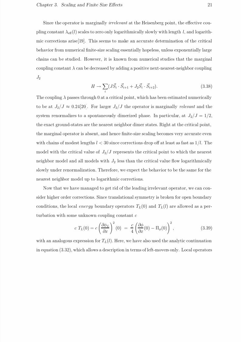
Chapter 3. Scaling and Finite Size Effects 21
Since the operator is marginally irrelevant at the Heisenberg point, the effective cou-
pling constant λeff (l) scales to zero only logarithmically slowly with length l, and logarith-
mic corrections arise[19]. This seems to make an accurate determination of the critical
behavior from numerical finite-size scaling essentially hopeless, unless exponentially large
chains can be studied. However, it is known from numerical studies that the marginal
coupling constant λ can be decreased by adding a positive next-nearest-neighbor coupling
J 2
H → i
(J S i · S i+1 + J 2 S i · S i+2). (3.38)
The coupling λ passes through 0 at a critical point, which has been estimated numerically
to be at J 2/J ≈ 0.24[20]. For larger J 2/J the operator is marginally relevant and the
system renormalizes to a spontaneously dimerized phase. In particular, at J 2/J = 1/2,
the exact ground-states are the nearest neighbor dimer states. Right at the critical point,
the marginal operator is absent, and hence finite-size scaling becomes very accurate even
with chains of modest lengths l < 30 since corrections drop off at least as fast as 1/l. The
model with the critical value of J 2/J represents the critical point to which the nearest
neighbor model and all models with J 2 less than the critical value flow logarithmically
slowly under renormalization. Therefore, we expect the behavior to be the same for the
nearest neighbor model up to logarithmic corrections.
Now that we have managed to get rid of the leading irrelevant operator, we can con-
sider higher order corrections. Since translational symmetry is broken for open boundary
conditions, the local energy boundary operators T L(0) and T L(l) are allowed as a per-
turbation with some unknown coupling constant c
c T L(0) = c
∂φL
∂x
2
(0) =c
4
∂φ
∂x(0) − Πφ(0)
2
, (3.39)
with an analogous expression for T L(l). Here, we have also used the analytic continuation
in equation (3.32), which allows a description in terms of left-movers only. Local operators

8/3/2019 Sebastian Eggert- Impurity Effects in Antiferromagnetic Quantum Spin-1/2 Chains
http://slidepdf.com/reader/full/sebastian-eggert-impurity-effects-in-antiferromagnetic-quantum-spin-12-chains 37/132
Chapter 3. Scaling and Finite Size Effects 22
are multiplied by a δ-function in the Hamiltonian density and will therefore be marginal
for scaling dimension d = 1 and relevant for d < 1. The operator in equation (3.39) has
dimension d = 2 for all values of J z and should give corrections of order 1/l to the finite
size spectrum, which will be discussed in the next section.
There is no such local operator for periodic boundary conditions, and the lowest
dimension bulk operator is T LT R of dimension d = 4, where T L,R have been defined in
equation (2.16). Corrections to the finite size spectrum of the periodic chain should
therefore be at least of order 1/l2. Note that the operator cos 4φ/R is also allowed by the
original symmetries of the Hamiltonian, but its scaling dimension of d = 4/πR2 makes it
much more irrelevant for all values of J z.
3.3 Finite-size Spectrum
As discussed above, there are four different fixed points to consider, corresponding to the
four different possible boundary conditions: periodic or open with even or odd length
(i.e. S z integer or half-odd-integer).
3.3.1 Periodic boundary conditions
We first consider the case of periodic boundary conditions on a spin-chain. This im-
plies periodic boundary conditions on φ as in equation (3.27) and determines the mode
expansion:
φ(x, t) = φ0 + Πvt
l+ Q
x
l+
∞n=1
1√4πn
e−
2πiln(vt+x)aLn + e−
2πiln(vt−x)aRn + h.c.
. (3.40)
This implies that φ has the mode expansion
φ(x, t) = φ0 + Qvt
l + Πx
l +
∞n=1
1√4πn
e−
2πi
l n(vt+x)aLn − e−2πi
l n(vt−x)aRn + h.c.
. (3.41)

8/3/2019 Sebastian Eggert- Impurity Effects in Antiferromagnetic Quantum Spin-1/2 Chains
http://slidepdf.com/reader/full/sebastian-eggert-impurity-effects-in-antiferromagnetic-quantum-spin-12-chains 38/132
Chapter 3. Scaling and Finite Size Effects 23
The aL,Rn ’s are bosonic annihilation operators. Π and Q are canonically conjugate to the
periodic variables φ0 and φ0, respectively. Hence their eigenvalues are quantized
Π = m/R, Q = 2πRS z, (3.42)
with
S z and m given in equation (3.27). Note, that φ is also periodic with radius 1/2πR,
as already mentioned in equation (2.18). The Hamiltonian can now be written as[21]
H = l0
Hdx =v
2
l0
Π2
φ +
∂φ
∂x
2
=v
2
Π2
l+
Q2
l+
2π
l
∞n=1
n
aL†n aLn + aR†n aRn
, (3.43)
with the resulting excitation spectrum
E =2πv
l
1
22πR2 (
S z)2 +
m2
2πR2 +
∞
n=1
n(mLn + mR
n ) . (3.44)
The corresponding wave-function is
ei(S z2πRφ0+mφ0/R)
∞n=1
(aL†n )m
Ln(aR†n )m
Rn |0 > . (3.45)
We see from equation (2.22) and (3.40) that site-parity takes m → −m and mLn ↔ mR
n .
It also multiplies the wave-function in equation (3.45) by eiπ(S z+m).
Here and in what follows, we always measure parity relative to that of the ground-
state. The ground-state parity itself for an even length chain is (
−1)l/2. At the point
J z = 0, R = 1/√
4π, this spectrum is that of free fermions with anti-periodic (periodic)
boundary conditions for even (odd) particle number. At the Heisenberg point J z =
J , R = 1/√
2π, the spin of left and right-movers is separately conserved and the z-
components are given by
S zL,R = (S z ± m)/2. (3.46)
S zL,R are either both integer or both half-odd-integer for even length l. For odd length
one quantum number is half-odd-integer while the other one is integer valued (i.e. S zLS zRis half-odd-integer valued).
8/3/2019 Sebastian Eggert- Impurity Effects in Antiferromagnetic Quantum Spin-1/2 Chains
http://slidepdf.com/reader/full/sebastian-eggert-impurity-effects-in-antiferromagnetic-quantum-spin-12-chains 39/132
Chapter 3. Scaling and Finite Size Effects 24
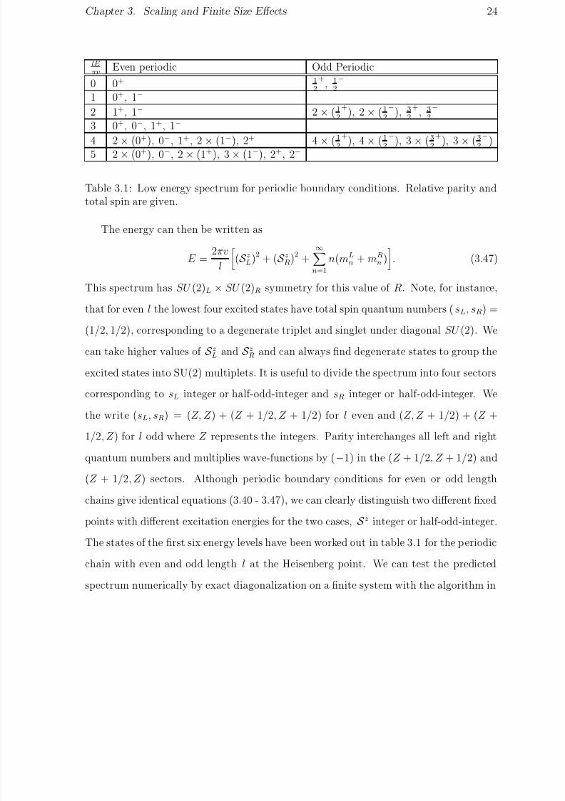
lE πv Even periodic Odd Periodic
0 0+ 12
+, 1
2
−
1 0+, 1−
2 1+, 1− 2 × (12
+), 2 × (1
2
−), 3
2
+, 3
2
−
3 0+, 0−, 1+, 1−
4 2 × (0+), 0−, 1+, 2 × (1−), 2+ 4 × (12
+
), 4 × (12−), 3 × (32
+
), 3 × (32−)5 2 × (0+), 0−, 2 × (1+), 3 × (1−), 2+, 2−
Table 3.1: Low energy spectrum for periodic boundary conditions. Relative parity andtotal spin are given.
The energy can then be written as
E =2πv
l
(S zL)2 + (S zR)2 +
∞n=1
n(mLn + mR
n )
. (3.47)
This spectrum has SU (2)L × SU (2)R symmetry for this value of R. Note, for instance,
that for even l the lowest four excited states have total spin quantum numbers (sL, sR) =
(1/2, 1/2), corresponding to a degenerate triplet and singlet under diagonal SU (2). We
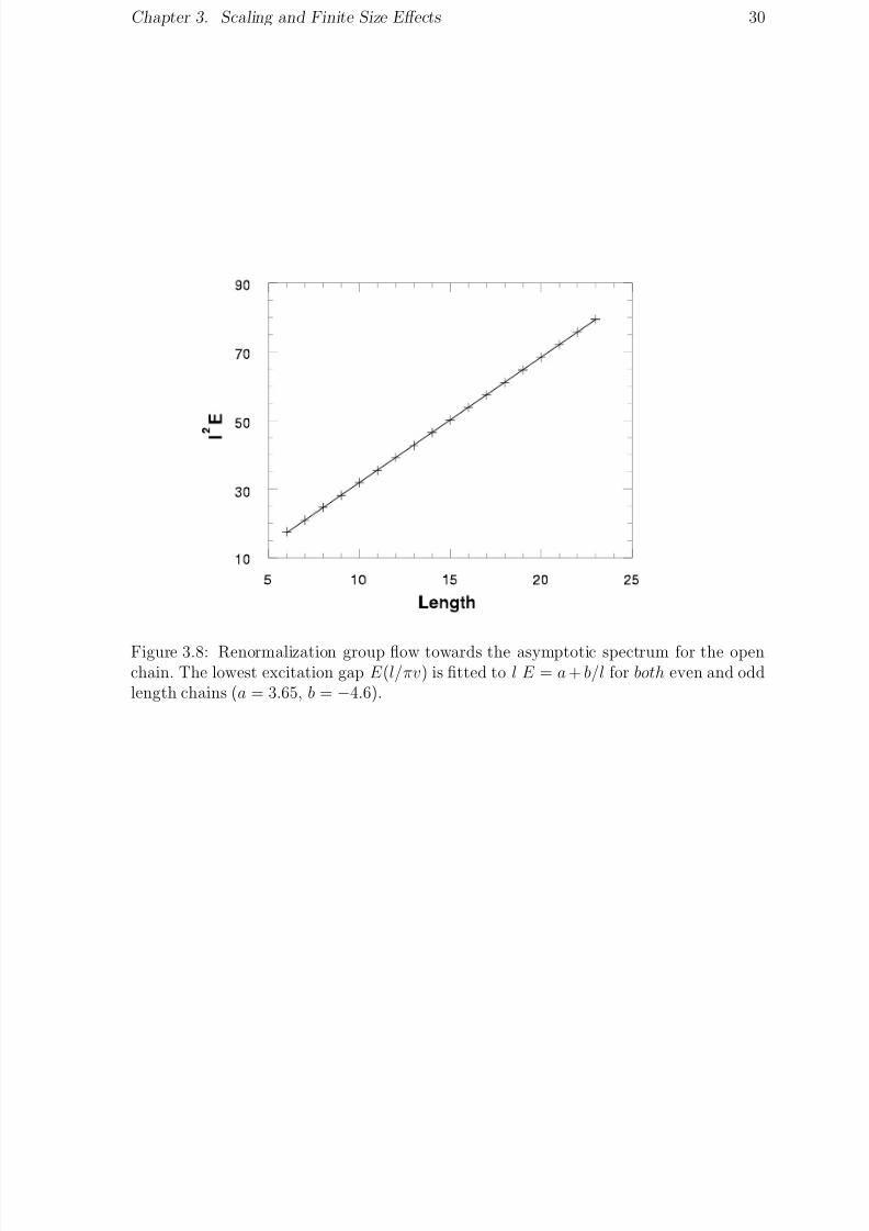
can take higher values of S zL and S zR and can always find degenerate states to group the
excited states into SU(2) multiplets. It is useful to divide the spectrum into four sectors
corresponding to sL integer or half-odd-integer and sR integer or half-odd-integer. We
the write (sL, sR) = (Z, Z ) + (Z + 1/2, Z + 1/2) for l even and (Z, Z + 1/2) + (Z +1/2, Z ) for l odd where Z represents the integers. Parity interchanges all left and right
quantum numbers and multiplies wave-functions by (−1) in the (Z + 1/2, Z + 1/2) and
(Z + 1/2, Z ) sectors. Although periodic boundary conditions for even or odd length
chains give identical equations (3.40 - 3.47), we can clearly distinguish two different fixed
points with different excitation energies for the two cases, S z integer or half-odd-integer.
The states of the first six energy levels have been worked out in table 3.1 for the periodic
chain with even and odd length l at the Heisenberg point. We can test the predicted
spectrum numerically by exact diagonalization on a finite system with the algorithm in

8/3/2019 Sebastian Eggert- Impurity Effects in Antiferromagnetic Quantum Spin-1/2 Chains
http://slidepdf.com/reader/full/sebastian-eggert-impurity-effects-in-antiferromagnetic-quantum-spin-12-chains 40/132
Chapter 3. Scaling and Finite Size Effects 25
Figure 3.3: Numerical low energy spectrum for periodic, even length l = 20 spin chain.The integer values El/πv of the numerically accessible states agree with the theoreticalpredictions. The velocity vπ = 3.69 was used (see figure 3.5).
appendix B. To get rid of the logarithmic correction, we chose a next nearest neighbor
coupling of J 2 = 0.24J as discussed above. Figures 3.3 and 3.4 show the excellent
agreement for all the states that were accessible with our algorithm (see appendix B).
Moreover, we can see in figure 3.5 that for this choice of the Hamiltonian, the corrections
to the spectrum E (l/π)v drop off exactly as 1/l2 as predicted in section 3.2 for periodic
boundary conditions.
3.3.2 Open boundary conditions
We now turn to the case of free boundary conditions on the spins corresponding to fixed
boundary conditions on φ, as in equation (3.30). The mode expansion is now:
φ(x, t) = 2πR 1
2+
S z x
l +
∞
n=1
1
√πnsin(
πnx
l) e−iπnt/lan + h.c. (3.48)

8/3/2019 Sebastian Eggert- Impurity Effects in Antiferromagnetic Quantum Spin-1/2 Chains
http://slidepdf.com/reader/full/sebastian-eggert-impurity-effects-in-antiferromagnetic-quantum-spin-12-chains 41/132
Chapter 3. Scaling and Finite Size Effects 26
Figure 3.4: Numerical low energy spectrum for periodic, odd length l = 19 spin chain(vπ = 3.69).
with S z integer (half-odd-integer) for l even (odd). The spectrum now takes the form[22]
E =πv
l
2πR2 (S z)2 +
∞n=1
nmn
. (3.49)
These results can also be derived when we consider a single left-moving boson on twice
the range −l to l and periodic or antiperiodic boundary conditions as in equation (3.33).
Note, that parity [i.e. x → l − x for fixed boundary conditions or x → −x for the
single boson] takes am → (−1)mam. It also multiplies wave-functions by (−1)S z
for l
even (for odd l we only have site-parity, which does not change the phase of the wave
function). Thus
P = (−1)
∞
p=0m2p+1+S z = (−1)
∞
p=1pmp+(S z)2 (3.50)
for l even. For l odd, (S z)2 − 1/4 is even, so we may write a similar formula:
P = (−1)∞
p=1 pmp+(S z)2−1/4. (3.51)

8/3/2019 Sebastian Eggert- Impurity Effects in Antiferromagnetic Quantum Spin-1/2 Chains
http://slidepdf.com/reader/full/sebastian-eggert-impurity-effects-in-antiferromagnetic-quantum-spin-12-chains 42/132
Chapter 3. Scaling and Finite Size Effects 27
Figure 3.5: Renormalization group flow towards the asymptotic spectrum of the periodicchain. The lowest excitation gap 0+, 1− is fitted to l E = a + b/l2 for even lengths(a = 3.69, b = 3.94).
At the Heisenberg point, this can be expressed in terms of the excitation energy
P = (−1)lE ex/vπ , (3.52)
where the ground-state energy of πv/4l, for l odd, is subtracted from E ex; i.e. the
energy levels are equally spaced, and the parity alternates. Again we measure parity
relative to the ground-state, which is (−1)l/2 or +1 for an even or odd-length open
chain, respectively. There is now a single SU (2) symmetry at the Heisenberg point
corresponding to two possible sectors with total spin s integer for l even or s half-odd-
integer for l odd.
The states of the first six energy levels have again been worked out in table 3.2 for open
boundary conditions at the Heisenberg point. We can test this spectrum numerically with
the algorithm in appendix B and find excellent agreement at the critical point J 2 = 0.24J

8/3/2019 Sebastian Eggert- Impurity Effects in Antiferromagnetic Quantum Spin-1/2 Chains
http://slidepdf.com/reader/full/sebastian-eggert-impurity-effects-in-antiferromagnetic-quantum-spin-12-chains 43/132
Chapter 3. Scaling and Finite Size Effects 28
lE πv
Even Open Odd Open
0 0+ 12
+
1 1− 12
−
2 0+, 1+ 12
+, 3
2
+
3 0−, 2
×(1−) 2
×(12
−), 3
2
−
4 2 × (0+), 2 × (1+), 2+ 3 × (12+), 2 × (3
2+)
5 2 × (0−), 4 × (1−), 2− 4 × (12
−), 3 × (3
2
−)
Table 3.2: Low energy spectrum for open boundary conditions. Relative parity and totalspin are given.
(see figures 3.6 and 3.7). Figure 3.8 shows that corrections to the energy gaps E (l/πv)
now drop off as 1/l, as expected for open boundary conditions. Note, however, that this
is a length dependent renormalization of the velocity v, since the corrections come fromthe boundary energy operator in equation (3.39). [see also the discussion before equation
(5.83)]. Therefore we estimate the velocity as vπ = 3.65 − 4.6/l in figures 3.6 and 3.7,
which gives good results.

8/3/2019 Sebastian Eggert- Impurity Effects in Antiferromagnetic Quantum Spin-1/2 Chains
http://slidepdf.com/reader/full/sebastian-eggert-impurity-effects-in-antiferromagnetic-quantum-spin-12-chains 44/132
Chapter 3. Scaling and Finite Size Effects 29
Figure 3.6: Numerical low energy spectrum for the open, even length l = 20 spin chain(vπ = 3.42).
Figure 3.7: Numerical low energy spectrum for the open, odd length l = 19 spin chain(vπ = 3.42).
8/3/2019 Sebastian Eggert- Impurity Effects in Antiferromagnetic Quantum Spin-1/2 Chains
http://slidepdf.com/reader/full/sebastian-eggert-impurity-effects-in-antiferromagnetic-quantum-spin-12-chains 45/132
Chapter 3. Scaling and Finite Size Effects 30
Figure 3.8: Renormalization group flow towards the asymptotic spectrum for the openchain. The lowest excitation gap E (l/πv) is fitted to l E = a + b/l for both even and oddlength chains (a = 3.65, b = −4.6).

8/3/2019 Sebastian Eggert- Impurity Effects in Antiferromagnetic Quantum Spin-1/2 Chains
http://slidepdf.com/reader/full/sebastian-eggert-impurity-effects-in-antiferromagnetic-quantum-spin-12-chains 46/132
Chapter 4
Impurities
We are now in the position to calculate the effect of any perturbation on the chain in
terms of our renormalization group and scaling analysis. Since we are able to express
perturbing spin operators in terms of the boson fields, we can determine the relevance of
the perturbation by looking at the corresponding scaling dimension.
Although a variety of possible perturbations can be considered[9], we will only consider
a local change of coupling constants between spins within the chain, which can model
many kinds of defects or impurities. We can obtain a more or less complete picture
by focusing on two simple cases, which can later be generalized with respect to their
symmetry properties: The perturbation of one coupling constant (“link”) within the
chain and the equal perturbation of two neighboring links. We will mainly consider
the isotropic model J z = J unless otherwise indicated, since it seems to be the most
interesting case experimentally[4].
4.1 One Perturbed Link
A generic local lattice distortion in a quasi one-dimensional spin compound could be
described by the small perturbation of one link in a periodic chain J S m · S m+1, as shown
in figure 4.9. Although such a perturbation has special link parity symmetry, we will argue
later that the following renormalization group analysis is valid for all local perturbation
that are not site parity symmetric. The S −mS +m+1 + S +mS −m+1 part of the interaction is
31

8/3/2019 Sebastian Eggert- Impurity Effects in Antiferromagnetic Quantum Spin-1/2 Chains
http://slidepdf.com/reader/full/sebastian-eggert-impurity-effects-in-antiferromagnetic-quantum-spin-12-chains 47/132
Chapter 4. Impurities 32
J’
Figure 4.9: A quantum spin chain with one altered link.
given by
S −mS +m+1 + S +mS −m+1 ≈ i(−1)m(ψ†LψR − h.c.), (4.53)
ignoring derivative terms of higher dimension as well as the uniform part which has the
same form as the free Hamiltonian density with scaling dimension d = 2. Using the
bosonization formula of equation (2.9) and rescaling the boson field following equation
(2.13), we obtain
S −mS +m+1 + S +mS −m+1 ≈ (−1)mconst. sinφ
R. (4.54)
which has scaling dimension d = 1/4πR2 and is therefore more relevant than the uniform
contribution for all positive values of J z.
The uniform part of S zmS zm+1 is known to have a scaling dimension of d = 2 from the
free Hamiltonian. The staggered part, i.e. the cross-term between uniform and staggered
parts of S z can be written in terms of the fermion currents:
[J L + J R] (m)
ψ†LψR(m + 1) + h.c.
+
ψ†LψR(m) + h.c.
[J L + J R] (m + 1) (4.55)
The individual terms can be written as a completely normal ordered four-Fermion oper-
ator together with an additional term from Wick-ordering of the form
J L(m)ψ†LψR(m + 1) → : ψ†
LψLψ†LψR : − i
2πψ†LψR. (4.56)
We can ignore all normal ordered terms since they reduce to irrelevant derivative oper-
ators. After combining all remaining terms together, we obtain the same operator as in
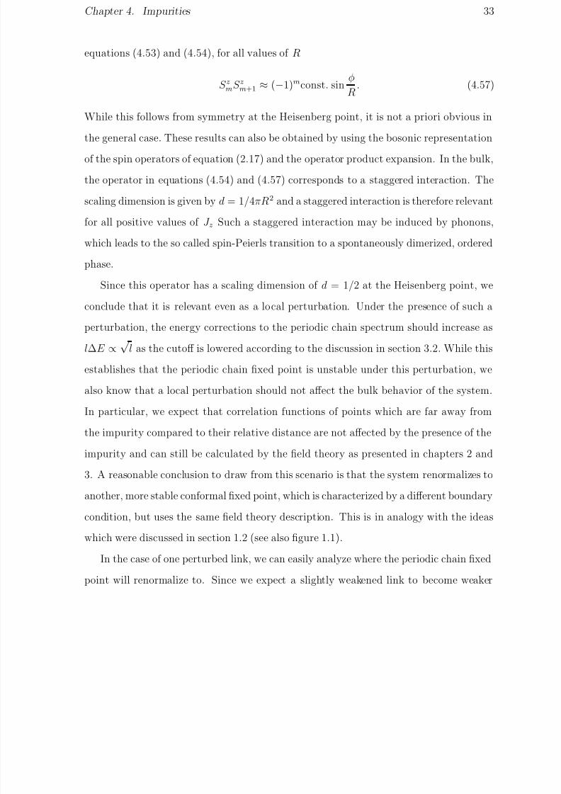
8/3/2019 Sebastian Eggert- Impurity Effects in Antiferromagnetic Quantum Spin-1/2 Chains
http://slidepdf.com/reader/full/sebastian-eggert-impurity-effects-in-antiferromagnetic-quantum-spin-12-chains 48/132
Chapter 4. Impurities 33
equations (4.53) and (4.54), for all values of R
S zmS zm+1 ≈ (−1)mconst. sinφ
R. (4.57)
While this follows from symmetry at the Heisenberg point, it is not a priori obvious in
the general case. These results can also be obtained by using the bosonic representation
of the spin operators of equation (2.17) and the operator product expansion. In the bulk,
the operator in equations (4.54) and (4.57) corresponds to a staggered interaction. The
scaling dimension is given by d = 1/4πR2 and a staggered interaction is therefore relevant
for all positive values of J z Such a staggered interaction may be induced by phonons,
which leads to the so called spin-Peierls transition to a spontaneously dimerized, ordered
phase.
Since this operator has a scaling dimension of d = 1/2 at the Heisenberg point, we
conclude that it is relevant even as a local perturbation. Under the presence of such a
perturbation, the energy corrections to the periodic chain spectrum should increase as
l∆E ∝√
l as the cutoff is lowered according to the discussion in section 3.2. While this
establishes that the periodic chain fixed point is unstable under this perturbation, we
also know that a local perturbation should not affect the bulk behavior of the system.
In particular, we expect that correlation functions of points which are far away fromthe impurity compared to their relative distance are not affected by the presence of the
impurity and can still be calculated by the field theory as presented in chapters 2 and
3. A reasonable conclusion to draw from this scenario is that the system renormalizes to
another, more stable conformal fixed point, which is characterized by a different boundary
condition, but uses the same field theory description. This is in analogy with the ideas
which were discussed in section 1.2 (see also figure 1.1).
In the case of one perturbed link, we can easily analyze where the periodic chain fixed
point will renormalize to. Since we expect a slightly weakened link to become weaker

8/3/2019 Sebastian Eggert- Impurity Effects in Antiferromagnetic Quantum Spin-1/2 Chains
http://slidepdf.com/reader/full/sebastian-eggert-impurity-effects-in-antiferromagnetic-quantum-spin-12-chains 49/132
Chapter 4. Impurities 34
under renormalization, the obvious guess for the stable fixed point is the chain with open
boundary conditions. A slightly strengthened link will grow as the cutoff is lowered, and
the two strongly coupled spins will eventually lock into a singlet which decouples from
the rest of the chain, so that we expect the stable fixed point again to be the open chain,
but now with two sites removed.
To test this assumption, we analyze the scaling dimension of a weak link across the
open ends. In the field theory, this is described by the product of two independent
boundary operators at the weakly coupled ends
S z1S zl ∝ ∂φL
∂x(1)
∂φL
∂x(l)
S +1 S −l ∝ e4πiRφL(1)e−4πiRφL(l), (4.58)
where we have used the boundary condition in equation (3.32). Since the scaling dimen-
sions of independent operators simply add, we find that the S z1S zl operator has a scaling
dimension of d = 2 independent of J z, while the S +1 S −l part has a scaling dimension of
d = 4πR2 which is also irrelevant as a local perturbation for all positive values of J z.
Thus, a weak link across the open ends renormalizes to zero. The open chain fixed point
is therefore indeed stable, and our assumptions above are consistent. At the Heisenberg
point all operators from a perturbation of one weak link across the open ends of a chainhave d = 2, and we expect that corrections to the open chain spectrum should flow to
zero as 1/l according to the discussion in section 3.2.
We can generalize these findings since the operator in equation (4.54) is always the
most relevant operator that can be produced by a local perturbation. A general pertur-
bation in the chain will therefore produce this operator unless special symmetries (e.g.
site parity) are present. Since relevant coupling constants will in general renormalize to
zero or infinity, we conclude that the periodic chain fixed point flows to the more stable
open chain fixed point as the temperature is lowered, if a local perturbation is present.

8/3/2019 Sebastian Eggert- Impurity Effects in Antiferromagnetic Quantum Spin-1/2 Chains
http://slidepdf.com/reader/full/sebastian-eggert-impurity-effects-in-antiferromagnetic-quantum-spin-12-chains 50/132
Chapter 4. Impurities 35
Figure 4.10: Flow away from the periodic chain fixed point due to one altered link foran odd length chain with 7 ≤ l ≤ 23. The lowest excitation gap 1
2
+, 1
2
−is fitted to
lE = a l1/2, which is the predicted scaling.
At the open chain fixed point, decoupled singlets may also be left over, and the effective
length of the chain may be reduced by an even number of sites.
We can test the scaling analysis from above numerically by looking at the energy
corrections l∆E of the energy gaps if a small perturbation is present. Since we want
to determine the scaling exponents accurately, all numerical simulations were done with
a next nearest neighbor coupling J 2 = 0.24J present, to avoid logarithmic corrections.
Perturbations from the periodic point should correspond to a scaling with l∆E ∝ √l as
mentioned above, which is indeed the case as shown in figure 4.10. A weak coupling across
open ends of the chain should lead to corrections to the spectrum l∆E ∝ 1/l + O(1/l2),
which is demonstrated nicely in figure 4.11.

8/3/2019 Sebastian Eggert- Impurity Effects in Antiferromagnetic Quantum Spin-1/2 Chains
http://slidepdf.com/reader/full/sebastian-eggert-impurity-effects-in-antiferromagnetic-quantum-spin-12-chains 51/132
Chapter 4. Impurities 36
Figure 4.11: Renormalization group flow towards the open chain fixed point due to oneweak link for an odd length chain with 7 ≤ l ≤ 23. The corrections to the lowestexcitation gap 1
2
+, 1
2
−is fitted to l∆E = a/l + b/l2, exhibiting the predicted 1/l scaling
up to higher order.
4.2 Two Perturbed Links
Since the operator in equation (4.54) does not respect site parity, we expect fundamentally
different behavior for site parity symmetric perturbations. As a generic case of a siteparity symmetric perturbation, we will consider the equal perturbation of two neighboring
links in the chain as shown in figure 4.12. Since the operator in equation (4.54) is
alternating, we immediately find that the most relevant site parity invariant operator is
the derivatived
dxsin
φ
R. (4.59)
Because the derivative increases the scaling dimension by one, this operator has scaling
dimension d = 1 + 1/4πR2, corresponding to d = 3/2 at the Heisenberg point. It is

8/3/2019 Sebastian Eggert- Impurity Effects in Antiferromagnetic Quantum Spin-1/2 Chains
http://slidepdf.com/reader/full/sebastian-eggert-impurity-effects-in-antiferromagnetic-quantum-spin-12-chains 52/132
Chapter 4. Impurities 37
J’ J’
Figure 4.12: A quantum spin chain with two altered links.
therefore irrelevant as a local perturbation. The uniform parts of the interaction have
dimension d = 2 as discussed before and are even more irrelevant.
The situation at the open chain fixed point is completely different, however, because
the open ends are now coupled to an external spin-1/2. The corresponding boundary
operators at l
S zl S zimp ∝ ∂φL
∂x(l)S zimp
S −l S +imp ∝ e−4πiRφL(l)S +imp (4.60)
now have scaling dimensions of d = 1 and d = 2πR2, respectively, since the impurity spin
is dimensionless. The boundary operators at x = 0 have corresponding expressions. The
coupling of open ends to an external spin is therefore found to be marginally relevant
at the Heisenberg point for anti-ferromagnetic coupling and marginally irrelevant forferromagnetic sign. We therefore expect the open chain to renormalize to the more
stable periodic chain if a site symmetric antiferromagnetic perturbation is present. The
chain effectively “heals” in this scenario.
These predictions can be tested numerically as before. Figure 4.13 shows the pre-
dicted scaling with 1/√
l for site symmetric perturbations from the periodic chain which
correspond to the scaling dimension of d = 3/2 as discussed in section 3.2. Figure 4.14
establishes the marginally relevant scaling for two weak anti-ferromagnetic links of the
open ends to an additional spin, while the marginally irrelevant case of two ferromagnetic

8/3/2019 Sebastian Eggert- Impurity Effects in Antiferromagnetic Quantum Spin-1/2 Chains
http://slidepdf.com/reader/full/sebastian-eggert-impurity-effects-in-antiferromagnetic-quantum-spin-12-chains 53/132
Chapter 4. Impurities 38
Figure 4.13: Flow towards the periodic chain fixed point for two altered antiferromagneticlinks. The 1
2
+, 12
−gap is fitted to lE = a/l1/2, which is the predicted scaling.
links is shown in figure 4.15. We can see that the logarithmic corrections increase and
decrease relative to the original coupling in the two cases. Since logarithmic scaling is
slow we have to also consider the irrelevant 1/l contribution in the two figures to obtain
a good fit. Although this three parameter fit is not entirely convincing, we can show that
the logarithmic contribution is essential to achieve a good fit as presented in figures 4.14
and 4.15. Even other three parameter fits which we tested cannot reproduce an equally
good fit without taking the logarithmic contribution into account.
4.3 Relation to Other Problems
Both link and site parity symmetric impurities that we have discussed above correspond
to special cases of models studied in the context of defects in one-dimensional quantumwires[23, 24]. In these papers spinless fermions were considered, which are equivalent

8/3/2019 Sebastian Eggert- Impurity Effects in Antiferromagnetic Quantum Spin-1/2 Chains
http://slidepdf.com/reader/full/sebastian-eggert-impurity-effects-in-antiferromagnetic-quantum-spin-12-chains 54/132
Chapter 4. Impurities 39
Figure 4.14: Flow away from the open chain fixed point for two weak antiferromagneticlinks. Corrections to the 12
+, 12
−gap are fitted to ∆E/E = (a+b/l+c ln l), demonstrating
relevant logarithmic scaling (ac > 0). The dotted line is the best fit for c = 0.
Figure 4.15: Flow towards the open chain fixed point for two weak ferromagnetic links.
Corrections to the 12+, 3
2− gap are fitted to ∆E/E = (a + b/l + c ln l), demonstrating
irrelevant logarithmic scaling (ac < 0). The dotted line is the best fit for c = 0.

8/3/2019 Sebastian Eggert- Impurity Effects in Antiferromagnetic Quantum Spin-1/2 Chains
http://slidepdf.com/reader/full/sebastian-eggert-impurity-effects-in-antiferromagnetic-quantum-spin-12-chains 55/132
Chapter 4. Impurities 40
to the xxz spin chain by the Jordan-Wigner transformation. The Heisenberg model
corresponds to a particular value of the repulsive interaction. The flow of a single modified
link to the open chain fixed point corresponds to the perfectly reflecting fixed point[23].
The “healing” discussed here corresponds to resonant tunneling[24]. In that work, it was
necessary to adjust one parameter to achieve the resonance condition (even with exact
site-Parity maintained). This parameter, a local chemical potential at the impurity site,
corresponds to an external magnetic field term h S z0 at the impurity site. In the spin
problem this is naturally set to zero by spin-rotation symmetry or time-reversal. Thus
resonance (healing) occurs without fine-tuning in the spin chain.
The case of two equally perturbed links J also has an interesting equivalent in the
two-channel Kondo problem[9], which has been realized independently in reference [25].
The description in the field theory language is completely analogous in the spin sector
of the Kondo problem if we identify the marginal coupling constants J of the spins at
the ends to the impurity spin in figure 4.12 with the Kondo coupling. The operators in
equation (4.60) can be identified with the spin currents that couple to the impurity in the
Kondo effect. The two ends of the spin chain are effectively independent of each other
and can be regarded as being described by two independent fields which play the role
of the two spin channels in the Kondo effect. The central spin in figure 4.12 represents
the impurity spin in the Kondo case. The overscreened Kondo problem is known to
renormalize to a non-trivial intermediate coupling fixed point[26], which corresponds to
the healed chain. For higher impurity spin, we recover the normal underscreening of
the Kondo problem in the spin chain model as well. It is, however, important to realize
that the spins in the chain are not equivalent to the spins of the electrons in the Kondo
problem, although the boson theory describing them is identical. The Kondo problem
additionally has charge excitations which do not couple to the impurity and can therefore
be neglected.

8/3/2019 Sebastian Eggert- Impurity Effects in Antiferromagnetic Quantum Spin-1/2 Chains
http://slidepdf.com/reader/full/sebastian-eggert-impurity-effects-in-antiferromagnetic-quantum-spin-12-chains 56/132
Chapter 4. Impurities 41
JK
JRKKY
JK
Figure 4.16: The equivalent spin chain model to the two impurity Kondo problem.
We can carry this analogy over to the single channel Kondo problem as well. In this
case, we imagine a semi-infinite spin chain with the open end coupled to the impurity
spin. As before, anti-ferromagnetic coupling J is marginally relevant, and the stable
fixed point is the open end with one extra site added (i.e. coupling J = J ). This
corresponds to the strongly coupled fixed point in the Kondo effect. We see that we
recover the famous π/2 phase shift of the fermions according to equation (2.4). As in the
Kondo effect, the effect of the renormalization can be described by the so called fusion
with a s = 1/2 primary field[8]. For higher impurity spin we obtain the correct size of
the effective left-over spin s−1/2 at the strong coupling fixed point J → ∞ as well, and
the usual underscreening of the Kondo problem is recovered[26].
Recently, it has been discovered that the two-impurity Kondo problem has an analogy
in a spin chain problem as well[8, 27]. In the equivalent spin chain model, two spin-1/2
impurities are coupled together with an RKKY coupling J RKKY , and each of the spins
is coupled separately to one of the open ends of the chain with a Kondo coupling J K
as shown in figure 4.16. In this case, both coupling constants are relevant in the weak
coupling limit, but a healed chain unstable fixed point J RKKY = J K = J separates the
two strong coupling stable phases. The two open ends of the spin chain now play the
role of the electron spin sectors at the two impurity sites in the Kondo problem. This
scenario is just another case of a link symmetric perturbation as discussed in section 4.1.
The two stable fixed points correspond to open chains with a possible decoupled singlet

8/3/2019 Sebastian Eggert- Impurity Effects in Antiferromagnetic Quantum Spin-1/2 Chains
http://slidepdf.com/reader/full/sebastian-eggert-impurity-effects-in-antiferromagnetic-quantum-spin-12-chains 57/132
Chapter 4. Impurities 42
and two sites removed if J RKKY scales to infinity. From the analysis above, we conclude
that the non-trivial fixed point should be unstable with scaling dimension d = 1/2.
These analogies are very useful since the spin chain Hamiltonians can be treated with
a variety of numerical techniques, which might give some better insight in correlation
functions and the size of the screening cloud in the Kondo effect. Moreover, it is easy
to visualize non-trivial fixed points for spin chain problems, and additional fixed points
may be found by simply adjusting the corresponding coupling constants.
8/3/2019 Sebastian Eggert- Impurity Effects in Antiferromagnetic Quantum Spin-1/2 Chains
http://slidepdf.com/reader/full/sebastian-eggert-impurity-effects-in-antiferromagnetic-quantum-spin-12-chains 58/132
Chapter 5
Susceptibilities
Now that a good theoretical understanding of the effect of impurities is established,
it is necessary to make clear predictions on how this can be seen in an experiment. As
indicated above, a µSR experiment on quasi one-dimensional magnetic compounds seems
to be a good choice to observe the predicted effects. In this setup, we expect that the
temperature dependence of the effective susceptibility at the muon site will be different
from the results of a conventional susceptibility measurement due to the renormalization
of the induced perturbation. In section 5.4 we will present the idea of the experimental
setup in more detail. But before we can make any definite predictions for an experiment,
it is necessary to take a closer look at the susceptibility of the spin chain and the effect
of perturbations on this susceptibility in general. In this chapter we primarily discuss
the field theory predictions for the susceptibility, while most of the Monte Carlo results
are presented in chapter 6.
The local susceptibility χi in the z-direction at site i is given by
χi(T ) ≡ ∂
∂h< S zi > |h=0 =
β 0
dτ j
< S z j (τ )S zi (0) > =1
T
j
< S z j S zi >, (5.61)
where h is the uniform magnetic field on the chain. We can drop the time dependence of
the expectation value, because the total spin-z S z commutes with the Hamiltonian. We
also have set the Bohr magneton times the gyromagnetic ratio gµB and the Boltzmann
constant kB
to one. The susceptibility is then measured in units of 1/J . This local
susceptibility will be different in the bulk and near a boundary since it is directly related
43

8/3/2019 Sebastian Eggert- Impurity Effects in Antiferromagnetic Quantum Spin-1/2 Chains
http://slidepdf.com/reader/full/sebastian-eggert-impurity-effects-in-antiferromagnetic-quantum-spin-12-chains 59/132
Chapter 5. Susceptibilities 44
to the correlation function. In some cases we will refer to the total susceptibility χtotal of
the chain, which is simply the sum of all local susceptibilities
χtotal ≡ i
χi (5.62)
The following calculations assume that we are in the scaling limit T J , l 1, so
that the field theory analysis is valid. A “thermal length” is naturally defined by v/T ,
and the width of the boundary layer is given by v/T K , where T K has been mentioned in
section 1.2. The meaning of the thermal length will become clearer shortly in equation
(5.64). For our analysis, we require that the system size l is very large compared to all
other scales in the system, in particular compared to v/T , i.e. Tl/v 1. The ultraviolet
cutoff can then always be reduced down to the temperature T .
5.1 Periodic Chain Susceptibility
Because the periodic chain is translationally invariant, the local susceptibility will be in-
dependent of the site index i. All spins in the chain therefore have the same susceptibility
χ, which defines the bulk susceptibility per site. Using equation (2.24) we find that the
sum over the S z correlation function in equation (5.61) is given by
j
< S z j S zi > =−1
16π3R2
l/2
−l/2dx
1
(x + vt)2+
1
(x − vt)2
. (5.63)
This expression is useful for calculating the susceptibility of the free boson model, i.e.
ignoring all irrelevant operators of the theory. Note, that the alternating part in equation
(2.24) does not contribute when summed over and can therefore be neglected. To get a
finite temperature result, we first make a Wick rotation to imaginary time τ , which we
associate with the inverse temperature β . A conformal transformation of the space time
continuum onto a cylinder with circumference β and length l → ∞ then yields the finite

8/3/2019 Sebastian Eggert- Impurity Effects in Antiferromagnetic Quantum Spin-1/2 Chains
http://slidepdf.com/reader/full/sebastian-eggert-impurity-effects-in-antiferromagnetic-quantum-spin-12-chains 60/132
Chapter 5. Susceptibilities 45
temperature correlation functions according to equation (A.107)
x ± vt → x ± ivτ → −ivβ
πsin
(ix vτ )π
vβ
. (5.64)
The bulk susceptibility for the free boson model is thus given by
χ =β
16π3R2
∞−∞
dx
vβ π
sin
(vτ − ix)πvβ
−2+
vβ π
sin
(vτ + ix)πvβ
−2 .
(5.65)
The integral can be done by the change of variables: u = tan τπβ and w = −i tan ixπ
vβ [28],
giving
I = ∞−∞
dx
vβ
πsin
(ix + vτ )π
vβ
−2
= 1−1
dwπ(1 + u2)
vβ (u + iw)=
2π
vβ , (5.66)
which is independent of τ or u as it should be since the total spin-z S z is conserved. The
final result for the bulk susceptibility per site of the free boson model is therefore[29]
χ =1
v(2πR)2, (5.67)
which is independent of temperature. This expression agrees with the zero temperature
expressions from the analytical Bethe ansatz[12]. We can improve this formula for the
spin chain in the field theory treatment by using perturbation theory in the irrelevant
operators, which will give us temperature dependent corrections to this expression. We
know from conformal invariance that finite size scaling should be analogous to finite
temperature scaling upon identifying l = v/T , so that we can use the same analysis as
in section 3.2.
5.1.1 Contributions from the leading irrelevant operator
The first order contribution to the bulk susceptibility from the leading irrelevant oper-ator cos(2φ/R) vanishes. The second order contribution is determined by our scaling

8/3/2019 Sebastian Eggert- Impurity Effects in Antiferromagnetic Quantum Spin-1/2 Chains
http://slidepdf.com/reader/full/sebastian-eggert-impurity-effects-in-antiferromagnetic-quantum-spin-12-chains 61/132
Chapter 5. Susceptibilities 46
arguments in section 3.2 and the scaling dimension d = 1/πR2, giving:
χ(T ) → 1
v(2πR)2+ const. T 2(1/πR
2−2). (5.68)
For 1/πR2 > 3, J z < J/2 the exponent will get replaced by 2, because in this case T LT R
from equation (2.16) is the leading irrelevant operator. For J z > J cos−1(π/5) ≈ .809J
we notice that the correction leads to an infinite slope at zero temperature.
At the Heisenberg point J z = J, R = 1/√
2π, we expect a logarithmic correction
according to section 3.2, because the leading irrelevant operator is marginal. These cor-
rections have been calculated by using the non-abelian bosonization of the spin chain[10],
in which the low energy effective field theory description is given by the k = 1 Wess-
Zumino-Witten (WZW) non-linear σ-model. The uniform part of the spin density is
given by the conserved current operators, J L, J R for left and right-movers:
S x ≈ J L(x) + J R(x). (5.69)
In the WZW model J L and J R are uncorrelated and their self-correlations are given by
< J aL(τ, x)J bL(0, 0) > =δab
8π2(vτ − ix)2
< J
a
R(τ, x
)J
b
R(0
,0)
>=
δab
8π2(vτ + ix)2 .(5.70)
The leading irrelevant operator is marginal and is now given by
−8π2v√3
g J L · J R. (5.71)
Using first order perturbation theory gives a correction to χ that involves four current
operators
χ = 12πv
+ vβ 28π2
g√3
l/2−l/2
dx l/2−l/2
dy < [J zL + J zR](0)[J zL + J zR](x) J L · J R(y) > . (5.72)

8/3/2019 Sebastian Eggert- Impurity Effects in Antiferromagnetic Quantum Spin-1/2 Chains
http://slidepdf.com/reader/full/sebastian-eggert-impurity-effects-in-antiferromagnetic-quantum-spin-12-chains 62/132
Chapter 5. Susceptibilities 47
Due to the fact that the left and right currents are uncorrelated, this expression factorizes
into a product of two two-point Green’s functions, one for left-movers and one for right-
movers according to equation (5.70). Using translational invariance, the spatial integrals
factorize into two independent integrals of the form of equation (5.66), giving
χ = 12πv
+ vβ 28π2g√3
l/2
−l/2dx
l/2
−l/2dy (< J zL(0)J zL(y) >< J zR(x)J zR(y) >
+ < J zR(0)J zR(y) >< J zL(x)J zL(y) >)
=1
2πv+ vβ 2
8π2g√3
1
8π2
2π
vβ
2
+
1
8π2
2π
vβ
2
=1
2πv+
g
v√
3. (5.73)
Again, the correction is naively temperature-independent, since g is dimensionless. How-
ever, this formula can be improved by replacing g with g(T ), the effective renormalized
coupling at temperature T . By integrating the lowest order β -function, g(T ) is given
by[19]
g(T ) ≈ g1
1 + 4πg1 ln(T 1/T )/√
3. (5.74)
Here g1 is the value of the effective coupling at some temperature T 1. Both g1 and g(T )
must be small for this formula to be valid. We may write this more compactly, as
g(T ) ≈ √34π ln(T 0/T )
, (5.75)
for some temperature T 0. Thus we obtain the leading T -dependence of χ
χ(T ) =1
2πv+
1
4πv ln(T 0/T ). (5.76)
As mentioned before, we can adjust g1 and T 0 by introducing a next nearest neighbor
coupling J 2, and at J 2 ≈ 0.24J we expect T 0 → ∞. However, for the model in equation
(1.1), J z = J, J 2 = 0, we expect a finite T 0 and a logarithmic divergence of the slope at
T = 0.

8/3/2019 Sebastian Eggert- Impurity Effects in Antiferromagnetic Quantum Spin-1/2 Chains
http://slidepdf.com/reader/full/sebastian-eggert-impurity-effects-in-antiferromagnetic-quantum-spin-12-chains 63/132
Chapter 5. Susceptibilities 48
T/J
0 0.5 1 1.5 2
0.1
0.12
0.14
Figure 5.17: χ(T ) from the Bethe ansatz. χ(0) = 1/Jπ2 is taken from equation (5.67).
As shown in figure 5.17, we have calculated the complete bulk susceptibility curve
for this case by use of the numerical Bethe ansatz of Takahashi[3, 30]. The bulk sus-
ceptibility obeys Curie’s law for large temperatures and goes through a maximum at
T ≈ 0.640824J, χ ≈ 0.147/J before the slope starts to increase again below an inflection
point at T ≈ 0.087J . We will use this curve as the unperturbed reference point for our
Monte Carlo simulations, which of course give identical results for this case, but with
larger error-bars. The existence of the maximum has been known for a long time[31] and
is used in experiments to establish the one-dimensional characteristics and determine the
coupling strength J [4, 5]. Our calculations give an additional prediction of an inflection
point at T ≈ 0.087J , which might be observable in some very highly one-dimensionalmaterials.

8/3/2019 Sebastian Eggert- Impurity Effects in Antiferromagnetic Quantum Spin-1/2 Chains
http://slidepdf.com/reader/full/sebastian-eggert-impurity-effects-in-antiferromagnetic-quantum-spin-12-chains 64/132
Chapter 5. Susceptibilities 49
0 0.02 0.04 0.06 0.08 0.10.1
0.105
0.11
0.115
T/J
Renormalization GroupBethe Ansatz
Figure 5.18: Field theory [equation (5.76), T 0 ≈ 7.7J ] versus Bethe ansatz results forχ(T ) at low temperature.
According to figure 5.18 our field theory predictions agree reasonably well with the
low temperature susceptibility behavior for a value of T 0 ≈ 7.7J . The curve starts to
deviate from our first order calculation as corrections of order (1/ ln T )3 and T 2 become
important. The magnitude of these corrections are not known, but ln T 0/T 1 should
be a sufficient condition for the validity of equation (5.76) which is consistent with figure
5.18. The divergent slope is not accessible by experiments, because of a finite ordering
temperature in quasi one-dimensional spin compounds, but the onset of this behavior
may have been observed in some cases[5].
The logarithmic scaling behavior has been observed before in numerical Bethe ansatz
calculations for finite size systems[19]. We can compare the result in the finite length

8/3/2019 Sebastian Eggert- Impurity Effects in Antiferromagnetic Quantum Spin-1/2 Chains
http://slidepdf.com/reader/full/sebastian-eggert-impurity-effects-in-antiferromagnetic-quantum-spin-12-chains 65/132
Chapter 5. Susceptibilities 50
0.015
0.02
0.025
0.03
0.035
0.04
0.045
0.05
0.055
10 100 1000
C o u p
l i n g g
Length
SingletTriplet
Ground StateSusceptibility
Renormalization Group
Figure 5.19: Estimates for the effective coupling g from lowest order perturbation theorycorrection to the finite-size energy of ground-state, first excited triplet state, first excitedsinglet state[19] and to the susceptibility, using l ↔ v/T . The renormalization groupprediction of equation (5.75) is also shown.

8/3/2019 Sebastian Eggert- Impurity Effects in Antiferromagnetic Quantum Spin-1/2 Chains
http://slidepdf.com/reader/full/sebastian-eggert-impurity-effects-in-antiferromagnetic-quantum-spin-12-chains 66/132
Chapter 5. Susceptibilities 51
limit lT/v → 0 from reference [19] directly with our calculation in the finite temperature
limit lT/v → ∞ upon identifying l = v/T , which appears to be the appropriate relation
(see figure 5.19).
It is possible to continue the expansion in the irrelevant operators to higher orders in
perturbation theory which will give higher order corrections in T . In the limit lT/v 1
the system size is always much larger than the finite temperature correlation length, and
we expect that finite length corrections to the periodic chain susceptibility are exponen-
tially small in lT/v. Because we have translational invariance we can therefore write the
total susceptibility of the periodic chain as χtotal = lχ(T ), where χ is independent of the
system size l up to exponentially small corrections.
5.2 Open Chain Susceptibility
The situation is somewhat different for the open chain since translational invariance is
broken. In this case it is possible to have an additional impurity contribution to the total
susceptibility which is independent of length
χimp ≡ liml→∞
i
χi − lχ
, (5.77)
where χi is now the local susceptibilities at site i of the open chain and χ is the bulksusceptibility per site from the previous section. This impurity susceptibility comes from
local irrelevant operators as in equation (3.39) in the field theory, which will be discussed
in section 5.2.2. The boundary condition condition itself does not contribute to the
uniform part of the susceptibility and therefore does not affect the impurity susceptibility
as will be explained at the end of section 5.2.1. An impurity susceptibility is also present
for any local perturbation on the periodic chain, and if no local operators were present,
neither fixed point in the field theory would have an impurity susceptibility contribution.
(Note, that the open chain in the lattice model corresponds to the open field theory
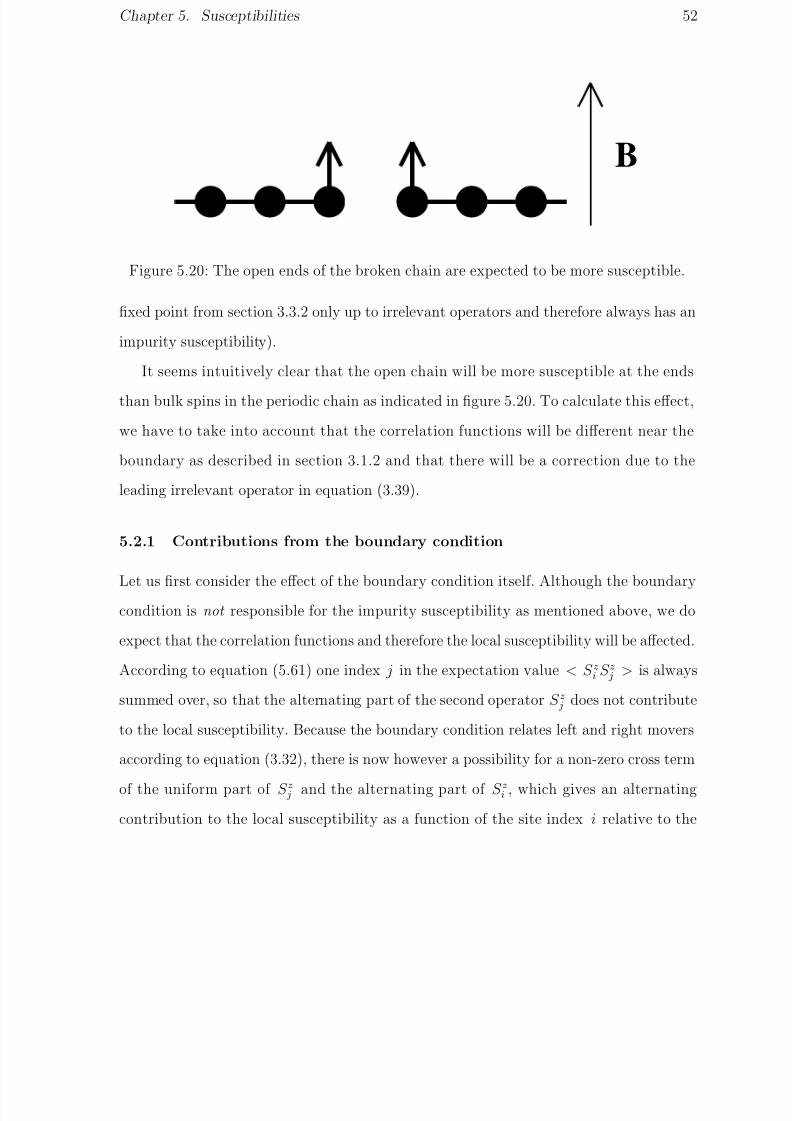
8/3/2019 Sebastian Eggert- Impurity Effects in Antiferromagnetic Quantum Spin-1/2 Chains
http://slidepdf.com/reader/full/sebastian-eggert-impurity-effects-in-antiferromagnetic-quantum-spin-12-chains 67/132
Chapter 5. Susceptibilities 52
B
Figure 5.20: The open ends of the broken chain are expected to be more susceptible.
fixed point from section 3.3.2 only up to irrelevant operators and therefore always has an
impurity susceptibility).
It seems intuitively clear that the open chain will be more susceptible at the ends
than bulk spins in the periodic chain as indicated in figure 5.20. To calculate this effect,
we have to take into account that the correlation functions will be different near the
boundary as described in section 3.1.2 and that there will be a correction due to the
leading irrelevant operator in equation (3.39).
5.2.1 Contributions from the boundary condition
Let us first consider the effect of the boundary condition itself. Although the boundarycondition is not responsible for the impurity susceptibility as mentioned above, we do
expect that the correlation functions and therefore the local susceptibility will be affected.
According to equation (5.61) one index j in the expectation value < S zi S z j > is always
summed over, so that the alternating part of the second operator S z j does not contribute
to the local susceptibility. Because the boundary condition relates left and right movers
according to equation (3.32), there is now however a possibility for a non-zero cross term
of the uniform part of S z j and the alternating part of S zi , which gives an alternating
contribution to the local susceptibility as a function of the site index i relative to the

8/3/2019 Sebastian Eggert- Impurity Effects in Antiferromagnetic Quantum Spin-1/2 Chains
http://slidepdf.com/reader/full/sebastian-eggert-impurity-effects-in-antiferromagnetic-quantum-spin-12-chains 68/132
Chapter 5. Susceptibilities 53
boundary. We therefore choose to separate the local susceptibility into a sum of an
alternating and a uniform part, corresponding to the alternating and uniform parts of
S z(x) in equation (2.17):
χx =1
T
dy < S z(x)S z(y) >
= 1T
< {S zuni(x) + (−1)xS zalt(x)}
dyS zuni(y) >
= χunix + (−1)xχalt
x (5.78)
This separation should be valid in the scaling limit, but at short distances it is of course
somewhat ambiguous (e.g. within a few lattice spacings of the boundary).
The corresponding expression for χaltx can be non-vanishing, because it is now ex-
pressed in terms of a three point Green’s function (without the boundary condition, it is
a vanishing two point function). After expressing the cosine in equation (2.17) in terms
of exponentials and using equation (3.32) we find
χaltx ∝ β
∞−∞
dy
e−i
√2πφL(x,t
)ei√2πφL(−x,t) ∂φL
∂x(y, t)
∝ β ∞−∞
dy
√2x
(y + vt − x − vt)(y + vt + x − vt), (5.79)
according to equation (A.108) with scaling dimensions d1 = d2 = 1/4 and d3 = 1 at the
Heisenberg point. Here, the index x measures the distance from the boundary in units of
the lattice spacing. We can evaluate this expression for finite T by using equation (5.64)
χaltx ∝
∞−∞
dy
vβ sinh 2πx
vβ
β sinh πvβ
(y + x + ivτ ) sinh πvβ
(y − x + ivτ )
∝ ∞−∞
dy
vβ sinh 2πx
vβ
β (cosh2 πvβ
(y + ivτ ) + sinh2 πvβ
(y + ivτ ) − cosh 2πxvβ
). (5.80)
This integral can be done if we set u = coth πvβ
(y + ivτ ), du = − πvβ
dysinh2 π
vβ(y+ivτ )
. The
final result is
χaltx ∝
1−1
du
vβ sinh 2πx
vβ
u2 + 1 − (u2 − 1) cosh 2πxvβ

8/3/2019 Sebastian Eggert- Impurity Effects in Antiferromagnetic Quantum Spin-1/2 Chains
http://slidepdf.com/reader/full/sebastian-eggert-impurity-effects-in-antiferromagnetic-quantum-spin-12-chains 69/132
Chapter 5. Susceptibilities 54
-0.6
-0.4
-0.2
0
0.2
0.4
0.6
0.8
0 5 10 15 20 25 30 35 40 45 50
L o c a l S u s c e p t i b
i l i t y
Sites
Figure 5.21: The local susceptibility near open ends from Monte Carlo simulations forβ = 15/J .
∝ x vβ sinh 2πx
vβ
. (5.81)
Note, that the alternating part may increase as we increase the distance x from the
boundary if we are at low temperatures. In particular at T = 0 we expect the alter-
nating part to increase exactly with√
x, which seems very counter-intuitive. (Note,
however, that experimental systems always contain the exponential drop-off from finite
temperatures.) This surprising effect has been checked by Monte Carlo simulations using
the algorithm in appendix C. The local susceptibility as a function of distance from the
open ends is shown in figure 5.21 for β = 15/J .
Using this Monte Carlo data, we can extract the uniform and alternating parts as
shown in figure 5.22 (as mentioned before this is somewhat ambiguous very close to the
boundary). The alternating part fits the predicted form 0.52(x+2)/
β sinh 2π(x + 2)/vβ
up to a constant α = 0.52 and a shift of two sites. This functional dependence holds
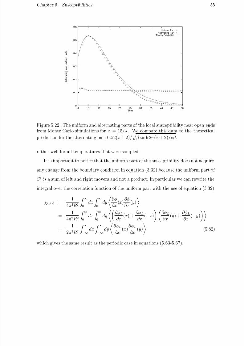
8/3/2019 Sebastian Eggert- Impurity Effects in Antiferromagnetic Quantum Spin-1/2 Chains
http://slidepdf.com/reader/full/sebastian-eggert-impurity-effects-in-antiferromagnetic-quantum-spin-12-chains 70/132
Chapter 5. Susceptibilities 55
0
0.1
0.2
0.3
0.4
0.5
0.6
0 5 10 15 20 25 30 35 40 45 50
A l t e r n a t i n g a n d U n i f o
r m P
a r t s
Sites
Uniform PartAlternating Part
Theory Prediction
Figure 5.22: The uniform and alternating parts of the local susceptibility near open endsfrom Monte Carlo simulations for β = 15/J . We compare this data to the theoretical
prediction for the alternating part 0.52(x + 2)/
β sinh 2π(x + 2)/vβ .
rather well for all temperatures that were sampled.
It is important to notice that the uniform part of the susceptibility does not acquire
any change from the boundary condition in equation (3.32) because the uniform part of
S zi
is a sum of left and right movers and not a product. In particular we can rewrite the
integral over the correlation function of the uniform part with the use of equation (3.32)
χtotal =1
4π2R2
∞0
dx ∞0
dy
∂φ
∂x(x)
∂φ
∂x(y)
=1
4π2R2
∞0
dx ∞0
dy
∂φL
∂x(x) +
∂φL
∂x(−x)
∂φL
∂x(y) +
∂φL
∂x(−y)
=1
2π2R2
∞−∞
dx ∞−∞
dy
∂φL
∂x(x)
∂φL
∂x(y)
(5.82)
which gives the same result as the periodic case in equations (5.63-5.67).

8/3/2019 Sebastian Eggert- Impurity Effects in Antiferromagnetic Quantum Spin-1/2 Chains
http://slidepdf.com/reader/full/sebastian-eggert-impurity-effects-in-antiferromagnetic-quantum-spin-12-chains 71/132
Chapter 5. Susceptibilities 56
5.2.2 Contributions from the leading irrelevant boundary operator
Although the local corrections due to the boundary condition are large, there will be
no impurity contribution to the total susceptibility since the alternating part does not
contribute under the integral and the uniform part does not change. This is in complete
agreement with the statement that the impurity susceptibility comes entirely from the
irrelevant boundary operators. In this section we will consider the contribution from the
leading irrelevant boundary operator in equation (3.39) with some unknown coupling
constant c. This boundary operator is present at each end, T L(0) and T L(l), but the two
operators are independent at the open chain fixed point and we may consider only the
operator at the origin and then generalize our findings for both ends.
The impurity correction in equation (5.77) to the susceptibility from T L(0) can be
calculated to first order with a simple trick, which has been used before in the context
of the Kondo problem[32]. The operator in equation (3.39) is proportional to the local
energy density, so that its effect to first order in perturbation theory is simply a length
dependent renormalization of the velocity v for any bulk quantity. In particular for the
bulk susceptibility to first order we can write
cv l
−l
dx l
−l
dy l
−l
dz δ(z)T L(z)∂φL
∂x
(x)∂φL
∂x
(y)→ c
lv l−l
dx l−l
dy l−l
dz
T L(z)
∂φL
∂x(x)
∂φL
∂x(y)
(5.83)
The integral over dz can now be reabsorbed to first order in the free Hamiltonian by
rescaling v → v(1 + c/l). In the thermodynamic limit, the effect for all translational
invariant quantities is then simply a rescaling of the temperature T → T /(1 + c/l) in
the partition function. In particular, the susceptibility per site can be calculated as a
function of the coupling constant c
χ(c, T ) =1
T
dx S zxS z0c,T

8/3/2019 Sebastian Eggert- Impurity Effects in Antiferromagnetic Quantum Spin-1/2 Chains
http://slidepdf.com/reader/full/sebastian-eggert-impurity-effects-in-antiferromagnetic-quantum-spin-12-chains 72/132
Chapter 5. Susceptibilities 57
=1
T
dx S zxS z0c=0,T/(1−c/l)
= χ
c = 0,
T
1 − c/l
1
1 − c/l
≈ χ +χimp
l. (5.84)
At T = 0 the correction corresponds to a shift cχ/l in the susceptibility per site. The
sum over all sites gives us the impurity correction to the susceptibility χimp ≈ cχ, which
is independent of length as it should be in the limit l → ∞ in equation (5.77).
Although this argument can give us the impurity correction to the total susceptibility,
it is not sufficient to predict the local corrections δχx due to the irrelevant operator in
equation (3.39). These can be calculated by doing first order perturbation theory in the
coupling constant c of the operator in equation (3.39)
δχx ∝ cβ 2 ∞−∞
dy
:
∂φL
∂x(0)
2:
∂φL
∂x(x)
∂φL
∂x(y)
, (5.85)
where we again only consider the boundary operator at 0 for simplicity. After replacing β
with an integral over dτ to take the proper time-correlations into account we can calculate
this expression by using the usual boson Green’s functions and Wick ordering:∂φL
∂x(x + ivτ )
∂φL
∂x(ivτ )
∂φL
∂x(y + ivτ )
∂φL
∂x(ivτ )
∝ (x − ivτ + ivτ )−2(y + ivτ − ivτ )−2. (5.86)
The finite temperature result for the local susceptibility correction can now be derived
from equation (5.64)
δχx ∝ cβ β 0
dτ
vβ
πsin
iπ(x − ivτ + ivτ )vβ
−2 ∞−∞
dy
vβ
πsin
π(iy − vτ + vτ )
vβ
−2
∝ c β 0
dτ
vβ
πsin
π(vτ − vτ + ix)
vβ
−2, (5.87)
where we also used equation (5.66). The integral over dτ gives −π cot[π(vτ − vτ +
ix)/βv]/v2β , which cancels for the given limits of integration and any finite x. For x = 0,
8/3/2019 Sebastian Eggert- Impurity Effects in Antiferromagnetic Quantum Spin-1/2 Chains
http://slidepdf.com/reader/full/sebastian-eggert-impurity-effects-in-antiferromagnetic-quantum-spin-12-chains 73/132
Chapter 5. Susceptibilities 58
however, we can get a non-zero value, which can be determined by doing the integral
over all x using equation (5.66). Therefore, the local correction to the uniform part of
the susceptibility is given by
δχx = cδ(x)χ. (5.88)
This result simply says that the impurity susceptibility χimp = cχ from equation (5.84) is
only added directly at the open ends, but we have to keep in mind that our field theory
analysis is valid only in the scaling limit so that we have to allow some finite width of
a few lattice spacings for the delta-function. In addition we still have the alternating
part from equation (5.81), which does not contribute when summed over x, but gives a
large local contribution. This picture agrees with the numerical findings in figure 5.22,
although the separation into the alternating and uniform part is somewhat ambiguous
right at the origin.
In chapter 4 we discussed some cases in which the boundary conditions did not only
correspond to the usual field theory fixed points, but also had sites removed or additional
decoupled impurity spins. In particular, the periodic chain with one strengthened link
renormalizes to the open chain with two sites removed. The impurity correction to the
susceptibility is now 2(c−1)χ, which may be positive or negative. Likewise, the unstable
fixed point in section 4.2 represents an open chain with a decoupled impurity spin. In
this case the impurity susceptibility has an additional Curie contribution proportional to
1/T from the decoupled spin.
5.3 Susceptibility Contributions from Perturbations
To study the effect of perturbations on the lattice Hamiltonian, it is useful to review
the renormalization group arguments which have been successfully applied in the Kondo
problems[32, 33]. These renormalization group arguments are directly related to the

8/3/2019 Sebastian Eggert- Impurity Effects in Antiferromagnetic Quantum Spin-1/2 Chains
http://slidepdf.com/reader/full/sebastian-eggert-impurity-effects-in-antiferromagnetic-quantum-spin-12-chains 74/132
Chapter 5. Susceptibilities 59
Kunstable stable
21
T/T = 1
Figure 5.23: Renormalization group analysis of the cross-over from an unstable to astable fixed point as the temperature is lowered.
discussion in section 1.2, which might be helpful in understanding the general ideas. At
the fixed points the system is completely scale invariant, but as soon as we introduce a
perturbation we expect that an energy scale T K is introduced, which simply corresponds
to the temperature where we expect the breakdown of perturbation theory. For stable
(unstable) fixed points the description of the free Hamiltonian is then approximately
valid for temperatures below (above) T K . If there is a renormalization from an unstable
to a stable fixed point, we expect the energy scales at the two fixed points to be related,
so that there is really only one energy scale T K that governs the cross-over.
In the case where a small perturbation creates all local operators near the fixed
point, we usually only have to consider the leading operator with the smallest scaling
dimension d, since all corrections due to the more irrelevant local operators vanish under
renormalization. We can then determine the relation between T K and the bare coupling
constant λ by a simple renormalization argument. According to the discussion in section
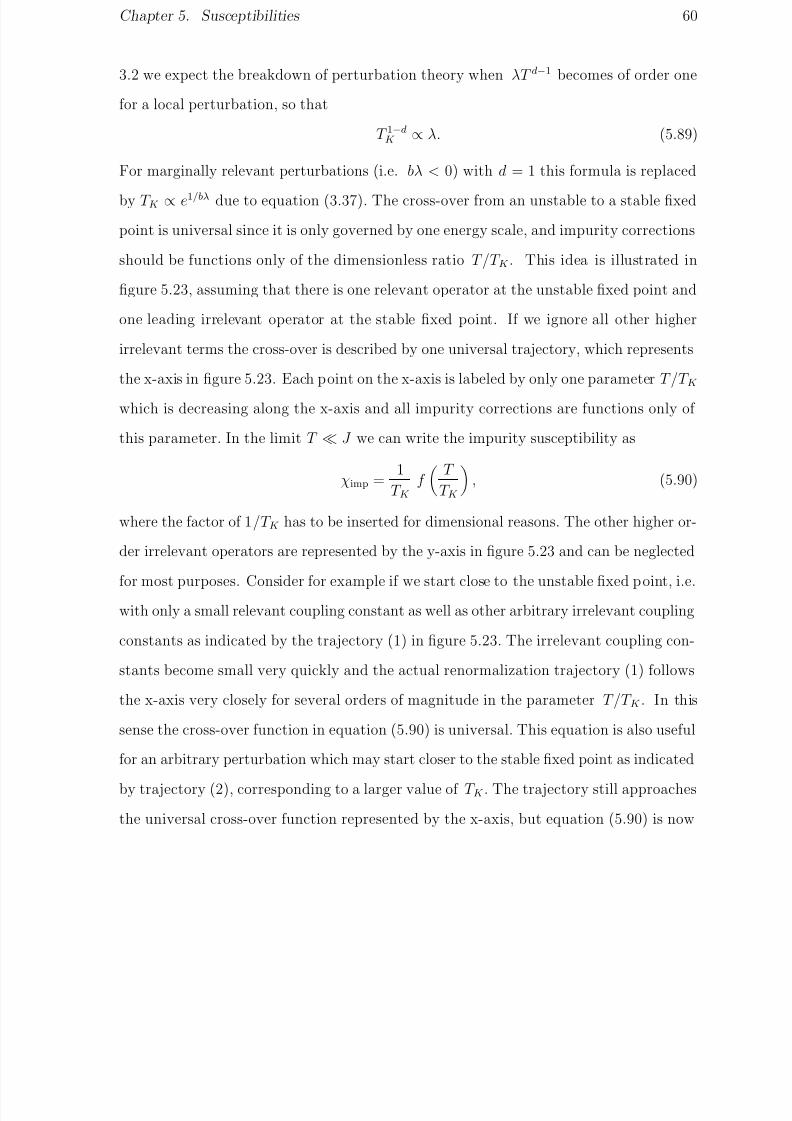
8/3/2019 Sebastian Eggert- Impurity Effects in Antiferromagnetic Quantum Spin-1/2 Chains
http://slidepdf.com/reader/full/sebastian-eggert-impurity-effects-in-antiferromagnetic-quantum-spin-12-chains 75/132
Chapter 5. Susceptibilities 60
3.2 we expect the breakdown of perturbation theory when λT d−1 becomes of order one
for a local perturbation, so that
T 1−dK ∝ λ. (5.89)
For marginally relevant perturbations (i.e. bλ < 0) with d = 1 this formula is replaced
by T K ∝ e1/bλ due to equation (3.37). The cross-over from an unstable to a stable fixed
point is universal since it is only governed by one energy scale, and impurity corrections
should be functions only of the dimensionless ratio T /T K . This idea is illustrated in
figure 5.23, assuming that there is one relevant operator at the unstable fixed point and
one leading irrelevant operator at the stable fixed point. If we ignore all other higher
irrelevant terms the cross-over is described by one universal trajectory, which represents
the x-axis in figure 5.23. Each point on the x-axis is labeled by only one parameter T /T K
which is decreasing along the x-axis and all impurity corrections are functions only of
this parameter. In the limit T J we can write the impurity susceptibility as
χimp =1
T K f
T
T K
, (5.90)
where the factor of 1/T K has to be inserted for dimensional reasons. The other higher or-
der irrelevant operators are represented by the y-axis in figure 5.23 and can be neglected
for most purposes. Consider for example if we start close to the unstable fixed point, i.e.with only a small relevant coupling constant as well as other arbitrary irrelevant coupling
constants as indicated by the trajectory (1) in figure 5.23. The irrelevant coupling con-
stants become small very quickly and the actual renormalization trajectory (1) follows
the x-axis very closely for several orders of magnitude in the parameter T /T K . In this
sense the cross-over function in equation (5.90) is universal. This equation is also useful
for an arbitrary perturbation which may start closer to the stable fixed point as indicated
by trajectory (2), corresponding to a larger value of T K . The trajectory still approaches
the universal cross-over function represented by the x-axis, but equation (5.90) is now

8/3/2019 Sebastian Eggert- Impurity Effects in Antiferromagnetic Quantum Spin-1/2 Chains
http://slidepdf.com/reader/full/sebastian-eggert-impurity-effects-in-antiferromagnetic-quantum-spin-12-chains 76/132
Chapter 5. Susceptibilities 61
valid only in an asymptotic region T /T K → 0.
This analysis fails if there is more than one leading irrelevant (or relevant) coupling
constant, since each coupling constant may set an independent cross-over energy scale.
In the case of two coupling constants c and λ with a leading scaling dimension d equation
(5.90) must be replaced by
χimp =1
T g
cT d−1, λT d−1
, (5.91)
This expression becomes equivalent to equation (5.90) if one of the coupling constants is
set to zero, which can be seen by using equation (5.89).
For the two-channel spin-1/2 Kondo problem the asymptotic behavior has been de-
termined to be[34, 35]
χimp ∝ ln(T K /T )/T K , (5.92)
for T T K . Curie’s law has to be recovered for T T K , so that χimp ∝ 1/T in
that regime. If the initial Kondo coupling J is weak, equation (5.92) reduces to χimp ∝ln(J/T )evπ/J
/J at low temperatures, which is less divergent than the unperturbed Curie
law behavior for any finite J . The scaling of T K with J follows from the discussion
that lead to equation (5.89) and the fact that the corresponding operator is marginally
irrelevant (b = 1/vπ).
5.3.1 Two perturbed links
The case of two weak links of the spin chain is very closely related to the two-channel
spin-1/2 Kondo effect as discussed in section 4.3, and we therefore expect the same
logarithmic divergence as in equation (5.92) of the impurity susceptibility at low temper-
atures. Starting from the weak coupling limit J
→0 equation (5.92) is valid for T
T K .
In this limit we can keep only the most divergent part of the impurity contribution (i.e.

8/3/2019 Sebastian Eggert- Impurity Effects in Antiferromagnetic Quantum Spin-1/2 Chains
http://slidepdf.com/reader/full/sebastian-eggert-impurity-effects-in-antiferromagnetic-quantum-spin-12-chains 77/132
Chapter 5. Susceptibilities 62
drop any constant terms) which results in the relation
χimp ∝ ln
J
T
evπ/J
J , (5.93)
since the marginal coupling constant of the “Kondo interaction” in equation (4.60) is
given by J to first order. The complete analytic form of the cross-over function is
difficult to determine, but we can easily see that we have to recover Curie law behavior
χimp ∝ 1/T in the opposite limit T T K , corresponding to a nearly free impurity spin.
The divergent part of the impurity susceptibility is expected to come mostly from the
central “impurity spin” in figure 4.12, which is clear from the analogy to the two-channel
Kondo effect and the analysis when J is small (i.e. when the “impurity spin” produces
a divergent Curie law susceptibility).
A small perturbation of two links from the periodic chain fixed point of δJ ≡ J − J
is the more interesting scenario for a µSR experiment. In this case there is no local
operator in the Hamiltonian at the unperturbed fixed point, and all local field theory
operators will have coupling constants of order δJ or higher. In this case we only have
to consider the leading irrelevant operator which is given in equation (4.59) with scaling
dimension of d = 3/2 at the Heisenberg point. We can use equation (5.89) to predict
the low temperature behavior of the impurity susceptibility for small perturbations δJ
on the lattice model. Since δJ produces the leading irrelevant operator to first order
λ ∝ δJ/J 3/2 + O(δJ 2) according to the analysis in section 4.2 we can write
χimp ∝ −δJ 2
J 3ln
T
J
, (5.94)
where the powers of J were inserted by dimensional analysis. This expression follows
directly from equations (5.89) and (5.92). Note, that we have inserted powers of J only
to relate coupling constants in the lattice models to coupling constants in the field theory
description with the correct units. However, J does not appear as an energy scale in the

8/3/2019 Sebastian Eggert- Impurity Effects in Antiferromagnetic Quantum Spin-1/2 Chains
http://slidepdf.com/reader/full/sebastian-eggert-impurity-effects-in-antiferromagnetic-quantum-spin-12-chains 78/132
Chapter 5. Susceptibilities 63
field theory description, because we lowered the ultraviolet cutoff all the way to the
temperature and J has been absorbed in the definition of the spin-wave velocity v.
In summary, the impurity susceptibility χimp increases monotonically with decreasing
temperature or increasing perturbation δJ .
5.3.2 One perturbed link
A similar analysis can be applied for the perturbation of one link from the periodic chain
δJ with the leading operator in equation (4.54) of dimension d = 1/2. By using perturba-
tion theory in the leading relevant operator with coupling constant of order λ ∝ δJ/√
J
we see that the leading order correction to the susceptibility is proportional to δJ 2/J .
This is because the first order contribution to the susceptibility < ∂ xφ∂ xφ sin φ/R > has
a vanishing expectation value, which can be seen by equation (A.105). Since T K ∝ δJ 2/J
according to equation (5.89), we conclude that the cross-over function in equation (5.90)
has an asymptotic behavior of f (r) → const/r2 as r → ∞. The simplest assumption for
small temperatures is f (0) = const.
There is one complication, however, which causes a problem near the open chain
fixed point, because there are now two dimension d = 2 leading irrelevant boundary
operators. The effect of the operator from equation (3.39) with coupling constant chas been discussed above, but the operator from equation (4.58) must also be taken
into account, which has a coupling constant λ ∝ J /J 2 for a weak link. The relative
magnitude of the two leading operators changes with J . For bare coupling constants
J → 0, which correspond to the open chain fixed point, the energy scale is therefore
determined by two independent parameters c and J . Therefore, we have to consider the
more general case of equation (5.91). We can expand g to first order by using the notion
that both first order corrections are independent of temperature according to equation

8/3/2019 Sebastian Eggert- Impurity Effects in Antiferromagnetic Quantum Spin-1/2 Chains
http://slidepdf.com/reader/full/sebastian-eggert-impurity-effects-in-antiferromagnetic-quantum-spin-12-chains 79/132
Chapter 5. Susceptibilities 64
(5.84) and the fact that f (0) = const. The resulting relation is
χimp =1
T g(cT,λT ) → cχ + const. J /J 2 (5.95)
where χ is the bulk susceptibility per site and c is the coupling constant of the local
operator T L in equation (3.39). We have also used λ ∝ J /J 2 and equation (5.84).
Equation (5.95) reduces to equation (5.90) as λ → 0 or c → 0.
These findings can be directly carried over to the case of a very large link J → ∞,
which also corresponds to the open chain fixed point but with two sites removed. In
this case there is an effective virtual coupling of order J 2/J across the open ends, which
now determines the leading order of λ and the same analysis as above can be applied.
However, it is not clear if the impurity susceptibility is positive or negative for large J as
discussed at the end of section 5.2.2, and therefore we cannot make any reliable scaling
arguments in this limit.
For a bare coupling constant δJ → 0, which corresponds to the periodic chain fixed
point, there is only one leading relevant operator with d = 1/2. Now, the energy scale is
determined by only one parameter λ ∝ δJ/√
J According to equation (5.89) this energy
scale becomes smaller as we approach the periodic chain T K ∝ δJ 2/J , which just repre-
sents an expected small cross-over temperature near the unstable fixed point. This hasa very interesting consequence for the zero temperature impurity susceptibility, because
equation (5.90) predicts χimp ∝ 1/T K ∝ J/δJ 2, which means a large impurity suscep-
tibility close to the periodic chain. The sign of the overall constant of proportionality
cannot be determined, because we are in the open chain fixed point regime T < T K and
the two leading irrelevant operators may partially cancel. This large T = 0 impurity
susceptibility is of little experimental relevance, however, because as soon as the temper-
ature is increased beyond δJ 2/J we find ourselves in the periodic fixed point regime, and
χimp ∝ T K /T 2 ∝ δJ 2/T 2 which gives a small impurity susceptibility as expected.
8/3/2019 Sebastian Eggert- Impurity Effects in Antiferromagnetic Quantum Spin-1/2 Chains
http://slidepdf.com/reader/full/sebastian-eggert-impurity-effects-in-antiferromagnetic-quantum-spin-12-chains 80/132
Chapter 5. Susceptibilities 65
5.4 A Muon Spin Resonance Experiment
Now that we have a good understanding of the local and impurity susceptibilities, it would
be nice to find experimental evidence for the predicted effects. As we mentioned in the
introduction one possible experiment to consider is a Muon Spin Resonance experiment on
quasi one-dimensional spin-1/2 compounds, in which the muon would perturb the system
and also probe the system locally at the impurity site[36]. The following discussion will
focus on this particular experiment, but it would of course be possible to use the Monte
Carlo results in chapter 6 for other kinds of experiments.
5.4.1 Experimental Setup
Positive muons are relatively long living particles (τ ≈ 2.2 × 10⁻⁶
sec) which carry apositive charge and a spin-1/2 and have about 200 times the mass of the electron. In a
µSR experiment, a low energy beam of muons is sent into the magnetic material to be
sampled. The beam is polarized, i.e. all muon spins are pointing in the same direction
perpendicular to a small applied magnetic field (see figure 5.24). The muons enter the
setup one at a time, and a timer is started for each muon. Once in the sample, the muons
quickly find chemically preferred sites, and the magnetic moment of the spin precesses in
the local magnetic field. Because weak interactions violate parity, the muon then decays
into a positron and two neutrinos in a way that the positron is most likely ejected in the
direction of the muon spin. The location where the positron hits one of the detectors
gives some information about the direction of the muon spin before the decay. Given
this direction and the time spent inside the sample, we can infer the strength of the local
magnetic field in which the muon precessed. Typically about 10,000-100,000 such events
per second can yield sufficient data within one or two hours. If a small external magnetic
field H is applied, this setup effectively measures the local susceptibility of the sample,
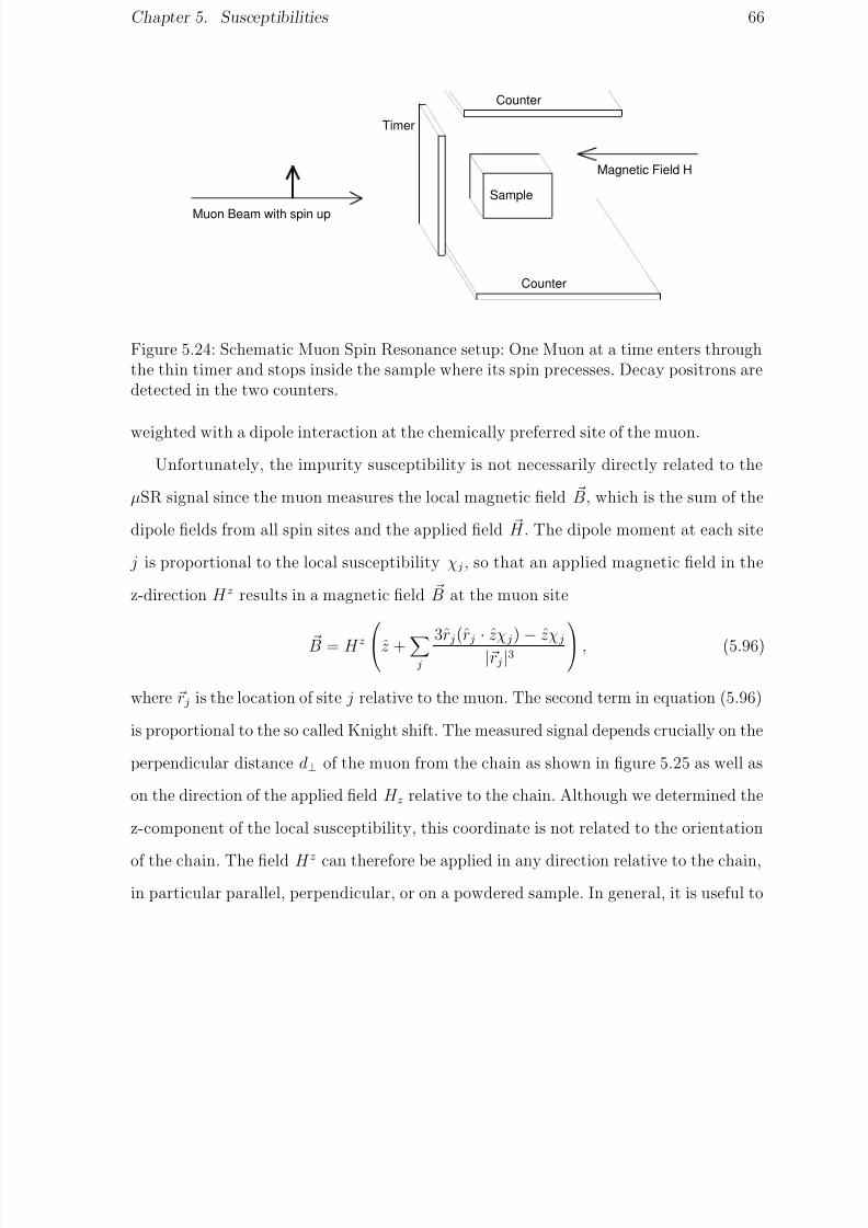
8/3/2019 Sebastian Eggert- Impurity Effects in Antiferromagnetic Quantum Spin-1/2 Chains
http://slidepdf.com/reader/full/sebastian-eggert-impurity-effects-in-antiferromagnetic-quantum-spin-12-chains 81/132
Chapter 5. Susceptibilities 66
Counter
Counter
Timer
Sample
Magnetic Field H
Muon Beam with spin up
Figure 5.24: Schematic Muon Spin Resonance setup: One Muon at a time enters throughthe thin timer and stops inside the sample where its spin precesses. Decay positrons aredetected in the two counters.
weighted with a dipole interaction at the chemically preferred site of the muon.
Unfortunately, the impurity susceptibility is not necessarily directly related to the
µSR signal since the muon measures the local magnetic field B, which is the sum of the
dipole fields from all spin sites and the applied field H . The dipole moment at each site
j is proportional to the local susceptibility χ j , so that an applied magnetic field in the
z-direction H z results in a magnetic field B at the muon site
B = H z
z + j
3r j(r j·
zχ j)−
zχ j
|r j |3
, (5.96)
where r j is the location of site j relative to the muon. The second term in equation (5.96)
is proportional to the so called Knight shift. The measured signal depends crucially on the
perpendicular distance d⊥ of the muon from the chain as shown in figure 5.25 as well as
on the direction of the applied field H z relative to the chain. Although we determined the
z-component of the local susceptibility, this coordinate is not related to the orientation
of the chain. The field H z can therefore be applied in any direction relative to the chain,
in particular parallel, perpendicular, or on a powdered sample. In general, it is useful to

8/3/2019 Sebastian Eggert- Impurity Effects in Antiferromagnetic Quantum Spin-1/2 Chains
http://slidepdf.com/reader/full/sebastian-eggert-impurity-effects-in-antiferromagnetic-quantum-spin-12-chains 82/132
Chapter 5. Susceptibilities 67
d j
d⊥
µ+
jr
Figure 5.25: The location of the muon relative to the chain for the link parity symmetriccase.
define an “effective” susceptibility at the muon site which is given by the second term in
equation (5.96) divided by the applied magnetic field
χeff ≡ j
χ j3(z · r j)2 − 1
|r j |3 (5.97)
The different cases for the various field directions will be discussed in chapter 6, but
for simplicity in this section we consider only the effective susceptibility χeff at the muon
site for a powdered sample as an rough indication of the muon signal
χeff = j
χ j|r j|3 , (5.98)
where we performed an integration over the solid angle in equation (5.97).
So far we have discussed how the muon is used as a magnetic probe in the system,
but a very important effect of the muon is of course the fact that it acts as an impurity
as well. Although we use the dipole interaction to probe the system, we do not expect
that this will produce a significant perturbation on the chain, since it is small compared
to the exchange interaction, the coulomb interaction, and even the interchain coupling.
The main effect of the muon therefore is a lattice distortion from inserting a positive

8/3/2019 Sebastian Eggert- Impurity Effects in Antiferromagnetic Quantum Spin-1/2 Chains
http://slidepdf.com/reader/full/sebastian-eggert-impurity-effects-in-antiferromagnetic-quantum-spin-12-chains 83/132
Chapter 5. Susceptibilities 68
charge in the system as shown in figure 5.25 for a link symmetric site. It is reasonable
to assume that the lattice distortion will drop off at least as fast as the derivative of the
coulomb force i.e. as 1/r3 and belongs to the same universality class as a short range
distortion. In cases where the muon binds directly to ions in the lattice or an electron
the distortion may be even more localized. The effect on the exchange interaction J can
only be roughly estimated by a previous experiment that observed a 20% shift in the
hyperfine levels under the influence of the muon[37], which indicates a distortion of the
orbitals and therefore a change of J of the same order of magnitude. Lattice distortions
due to the muon may be in excess of 30%[38]. But even small distortions are bound to
create large changes in J , since it is known from studies on MnO[39] that δJ/J can be
more than one order of magnitude larger than the lattice distortion δa/a, where a is the
lattice spacing.
The magnitude and range of the perturbation will vary from material to material. It
is therefore most appropriate to use a generic model for link and site parity symmetric
perturbations, corresponding to one or two equally perturbed links of various magnitude.
Although it seems unlikely that the effect of the muon will exactly correspond to one of
those two perturbations, it is reasonable to expect that it creates a symmetric pertur-
bation. All preceding calculations do not require the knowledge of the actual form of
the perturbation, but only refer to the leading operator, which is directly related to the
symmetry properties of the perturbation. The renormalization group arguments should
therefore be valid for any generic site or link parity symmetric perturbation of the muon.
Unfortunately, the muon will primarily probe the “non-universal” boundary region,
which is not accessible by the field theory analysis and does depend on the specific
form of the perturbation. As a first attempt to calculate the effective susceptibility
quantitatively, we consider the cases of either two equally or one perturbed isotropic
couplings. Depending on the results of the proposed experiment[36], further simulations

8/3/2019 Sebastian Eggert- Impurity Effects in Antiferromagnetic Quantum Spin-1/2 Chains
http://slidepdf.com/reader/full/sebastian-eggert-impurity-effects-in-antiferromagnetic-quantum-spin-12-chains 84/132
Chapter 5. Susceptibilities 69
may be appropriate. The Monte Carlo data for the µSR experiment in section 6.2 should
therefore be taken as a rough estimate of the predicted effects. The detailed signal of
an experiment may look different, but we expect that the size of the corrections to the
local susceptibility will be determined by the renormalization effects and the alternating
operator, both of which are large.
5.4.2 Field Theory Analysis
Let us first consider the site parity symmetric case, which is modeled by two adjacent,
equally perturbed links. We concluded that in this case the logarithmically divergent
part of the impurity susceptibility comes primarily from the local susceptibility of the
central “impurity” spin in figure 4.12. This followed from the analogy to the two channel
Kondo effect and should be true for small J or for T > T K . Since this central spin is
also the closest to the muon we expect that the µSR signal is directly related to the
impurity susceptibility. The induced alternating susceptibility in the chain for small J
will be secondary because the affected sites are further away and the magnitude of δχi
will be smaller. Nevertheless, this alternating part is interesting from a theoretical point
of view and we expect interesting behavior in the local susceptibility from the Monte
Carlo simulations. For small coupling J and temperatures T > T K we expect openchain behavior with an induced alternating part from the boundary condition, which is
positive at the ends. The interesting effect occurs when we lower the temperature or
increase the coupling J so that we approach the periodic chain fixed point. The central
impurity spin is then considered part of the chain, but still has a large local susceptibility
(i.e. a large < S z > expectation value when a small magnetic field is applied). But since
the spin is now considered part of a periodic chain equation (2.24) is valid and this large
< S z > expectation value propagates into the chain. In particular it induces a large
alternating part which is of opposite sign of that from the boundary condition, so that

8/3/2019 Sebastian Eggert- Impurity Effects in Antiferromagnetic Quantum Spin-1/2 Chains
http://slidepdf.com/reader/full/sebastian-eggert-impurity-effects-in-antiferromagnetic-quantum-spin-12-chains 85/132
Chapter 5. Susceptibilities 70
we should be able to observe a cross-over from a regime where the boundary alternating
part dominates to a regime where the induced alternating part from the impurity spin
dominates. This behavior is discussed again with the Monte Carlo data in section 6.1.3
and figures 6.35 - 6.38.
A similar analysis can be applied for the case corresponding to one weak link in
the chain. We now expect that the two sites connected by the weak link dominate the
Knight shift. Those two sites have a large contribution to the uniform part of the local
susceptibility which is directly related to the impurity susceptibility according to equation
(5.88). However, we now also have to consider the effect of the large alternating part from
equation (5.81), which is of similar magnitude at the two sites. We are somewhat saved
by the fact that there is no cancellation of the two parts in this case and the alternating
part adds to the uniform contribution, so that the muon signal is roughly related to the
impurity susceptibility. If the link is strengthened the effective susceptibility in equation
(5.98) is always decreased because the two closest sites in figure 4.9 lock into a singlet at
low temperatures. Their local susceptibility will therefore be lower and this behavior will
dominate the effective susceptibility at the muon site. In this case it is not even clear
if the impurity susceptibility (which involves a sum over the complete chain) should be
positive or negative as indicated at the end of section 5.2.2. The effect of the perturbation
on the effective susceptibility should be large in all scenarios.
Note, that only the uniform part of the local susceptibility is dependent on the bare
coupling constant J while the alternating part is produced by the boundary condition
itself. The uniform part of the local susceptibility of the first few sites near the impurity
therefore should depend on the coupling constant J while the alternating part far away
should be independent at a fixed temperature (provided that J is small enough that the
open fixed point description is valid).

8/3/2019 Sebastian Eggert- Impurity Effects in Antiferromagnetic Quantum Spin-1/2 Chains
http://slidepdf.com/reader/full/sebastian-eggert-impurity-effects-in-antiferromagnetic-quantum-spin-12-chains 86/132
Chapter 6
Monte Carlo Results
The field theory treatment of the spin chain is very useful in predicting impurity effects
in quasi one-dimensional spin systems, but unfortunately this analysis cannot give us
any quantitative results for the experiments other than the scaling behavior in certain
limits. To tie the theoretical predictions to experiments it is therefore useful to have an
independent method of determining the quantitative effects of impurities. With the help
of the standard quantum Monte Carlo algorithm as described in appendix C we are able
to present these quantitative results, which can provide experimentalists with an initial
estimate of the magnitude of the effects and should also be helpful in separating out the
impurity contribution from other effects in the analysis of the experimental data.
6.1 Impurity Susceptibility Effects
Monte Carlo simulations always have an inherent statistical error associated with them.
In our case there is also a critical slowing down at low temperatures, so that the simu-
lations do not produce useful data for T < J/15 (see also appendix C). Although the
local susceptibilities and the µSR signal have been determined with reasonable accuracy,
the error bars of the impurity susceptibility are rather large. Since we have to sum all
local susceptibilities to calculate the overall impurity susceptibility, its error bars are
larger by a factor of the square root of the system size (i.e. one order of magnitude for
l ≈ 48 − 128). As an example, the temperature dependence of the open chain impurity
susceptibility and the local susceptibility correction (χ1 − χ) of the site closest to the
71

8/3/2019 Sebastian Eggert- Impurity Effects in Antiferromagnetic Quantum Spin-1/2 Chains
http://slidepdf.com/reader/full/sebastian-eggert-impurity-effects-in-antiferromagnetic-quantum-spin-12-chains 87/132
Chapter 6. Monte Carlo Results 72
impurity have been plotted in figure 6.26. The error bars of the local susceptibility are
much smaller, but unfortunately we can normally not extract the impurity susceptibility
directly from this quantity, because it also contains an unspecified alternating contri-
bution, which is apparently large. As predicted, the impurity susceptibility seems to
approach a constant positive value as T → 0. The local susceptibility at the first site
seems to be roughly related to this impurity susceptibility, but with smaller error bars.
The alternating contribution adds so that the signal at the first site is larger than the
uniform impurity susceptibility. However, the accurate determination of the zero temper-
ature impurity susceptibility is difficult, and the computer simulations for this quantity
can only give a trend and a consistency check of our analysis in sections 5.3.1 and 5.3.2.
Figure 6.26 gives a good estimate for the approximate error bars in general for the local
and impurity susceptibilities, respectively. To make the presentation of the Monte Carlo
data less confusing, the error bars of figures 6.27 - 6.38 in this section have been omitted
and should simply be taken from figure 6.26.
6.1.1 One weak link
Figure 6.27 shows the impurity susceptibility of an open chain which has been slightly
perturbed with a coupling J across the open ends. The large error bars as given infigure 6.26 make this Monte Carlo data not unambiguous, but the findings seem to be
consistent with equation (5.95) which predicts a change in the impurity susceptibility
proportional to J . We believe that the apparent crossing for some parameters J is only
produced by the large uncertainties.
The more interesting case is a small weakening by δJ of one link from the periodic
chain. At intermediate temperatures T K < T < J the impurity susceptibility should be
proportional to δJ 2 according to section 5.3.2. Figure 6.28 confirms an increase of the
impurity susceptibility in this temperature regime, but higher order irrelevant operators

8/3/2019 Sebastian Eggert- Impurity Effects in Antiferromagnetic Quantum Spin-1/2 Chains
http://slidepdf.com/reader/full/sebastian-eggert-impurity-effects-in-antiferromagnetic-quantum-spin-12-chains 88/132
Chapter 6. Monte Carlo Results 73
0
0.05
0.1
0.15
0.2
0.25
0.3
0.35
0.4
0.45
0.5
0 0.2 0.4 0.6 0.8 1
I m p u r i t y S u s c e
p t i b i l i t y
T/J
Impurity SusceptibilityCorrection to the local Susceptibility at the first site
Figure 6.26: The open chain impurity susceptibility as a function of temperature. Thesolid line is only drawn for visual guidance and does not necessarily reflect an accurateestimate.

8/3/2019 Sebastian Eggert- Impurity Effects in Antiferromagnetic Quantum Spin-1/2 Chains
http://slidepdf.com/reader/full/sebastian-eggert-impurity-effects-in-antiferromagnetic-quantum-spin-12-chains 89/132
Chapter 6. Monte Carlo Results 74
0
0.05
0.1
0.15
0.2
0.25
0.3
0 0.2 0.4 0.6 0.8 1
I m p u r i t y S u s c e p t i b i l i t y
T/J
J’= 0J’= 0.1JJ’=0.25JJ’= 0.5J
Figure 6.27: The impurity susceptibility for a small coupling J across the open ends asa function of temperature.
seem to alter the scaling dependence, which appears to be linear with δJ . Perturbation
theory in the lattice model actually does predict a linear dependence on δJ . The scaling
prediction with δJ 2 comes from perturbation theory in the field theory Hamiltonian with
the leading relevant operator only, which does not seem to be valid at the intermediate
temperatures 0.3J < T < J . Other irrelevant operators [e.g. T L(0) from equation (3.39)]become important in this regime, which do contribute to first order in perturbation theory
and also have coupling constants of order δJ . Hence, the linear change with δJ in the
impurity susceptibility is consistent with the field theory analysis.
For temperatures below the small cross-over scale T K ∝ δJ 2/J we expect that the
impurity susceptibility should go as J/δJ 2. If a negative proportionality constant is
assumed, the numerical findings are consistent with this prediction. However, our Monte
Carlo data is not good enough to give a reliable confirmation of the sharp cross-over at

8/3/2019 Sebastian Eggert- Impurity Effects in Antiferromagnetic Quantum Spin-1/2 Chains
http://slidepdf.com/reader/full/sebastian-eggert-impurity-effects-in-antiferromagnetic-quantum-spin-12-chains 90/132
Chapter 6. Monte Carlo Results 75
-0.12
-0.1
-0.08
-0.06
-0.04
-0.02
0
0.02
0.04
0.06
0.08
0.1
0 0.2 0.4 0.6 0.8 1
I m p u r i t y S u s c e p t i b i l i t y
T/J
J’=0.75JJ’= 0.9J
Figure 6.28: The impurity susceptibility for a small perturbation δJ of one link in thechain as a function of temperature. The solid lines are only drawn for visual guidanceand do not necessarily reflect an accurate estimate.
very low temperatures as we approach the periodic chain.
6.1.2 Two weak links
As discussed in section 5.3.1 we expect a divergent impurity susceptibility as T
→0
for any finite weakening of two adjacent links. For small perturbations δJ , equation
(5.94) predicts a scaling of the impurity susceptibility with δJ 2, which is consistent with
figure 6.29. However, the large error bars in figure 6.26 also make this Monte Carlo data
somewhat ambiguous. It is therefore instructive to look at the correction to the local
susceptibility of the central spin closest to the impurity in figure 4.12, because of the
smaller error bars associated with local susceptibilities. This central spin is equivalent
to the “impurity spin” in the Kondo problem and presumably carries the divergent part
of the impurity susceptibility. Figure 6.30 seems to indicate a saturation of the impurity

8/3/2019 Sebastian Eggert- Impurity Effects in Antiferromagnetic Quantum Spin-1/2 Chains
http://slidepdf.com/reader/full/sebastian-eggert-impurity-effects-in-antiferromagnetic-quantum-spin-12-chains 91/132
Chapter 6. Monte Carlo Results 76
susceptibility at T K ≈ 0.3J , δJ = 0.1J , which might be interpreted as cross-over from
a Curie-law behavior to a weaker logarithmic scaling. This would imply that the cross-
over temperatures for all other coupling constants considered are too small to observe,
because T K ∝ J/δJ 2. This would indicate that the “healing” process as described in
section 4.2 is very slow, as might be expected from the dimensionalities of the leading
operators, which are only marginal relevant and only weakly irrelevant at the two fixed
points. Figure 6.30 also seems consistent with equation (5.94).
Figure 6.31 shows the impurity susceptibility for small bare coupling constants J
to the impurity spin. It is again instructive to look at the local susceptibility of the
“impurity spin”, which can be compared with the Curie-law behavior of a completely
decoupled spin as shown in figure 6.32. Since the cross-over temperature is much lower
than the lowest accessible temperature, we cannot observe the predicted behavior with
−evπ/J
ln T , but the Monte Carlo data certainly is consistent with this scaling function.
6.1.3 Alternating Parts
Predictions for the alternating part of the impurity susceptibility can be tested much more
easily, because it only involves local susceptibilities with much smaller uncertainties. Thefunctional dependence of the alternating part has already been confirmed in figure 5.22,
but it is interesting to note that the strong staggered behavior persists even for small
perturbations of one link in the periodic chain as shown in figure 6.33. In fact, we expect
the staggered part to be asymptotically independent of the bare coupling constant in
the limit T T K and x > v/T K , which is confirmed in figure 6.34. At T = J/15, the
staggered part is only very weakly dependent on J as long as J is small (which also
means v/T K is small). For perturbations of the order of J ≈ 0.5J we find a different
amplitude at short distances from the boundary, but far away from the boundary all

8/3/2019 Sebastian Eggert- Impurity Effects in Antiferromagnetic Quantum Spin-1/2 Chains
http://slidepdf.com/reader/full/sebastian-eggert-impurity-effects-in-antiferromagnetic-quantum-spin-12-chains 92/132
Chapter 6. Monte Carlo Results 77
-0.04
-0.02
0
0.02
0.04
0.06
0.08
0.1
0.12
0 0.2 0.4 0.6 0.8 1
I m p u r i t y S u s c e p t i b
i l i t y
T/J
J’=0.75JJ’= 0.9J
Figure 6.29: The impurity susceptibility for a small perturbation δJ of two links in thechain as a function of temperature.
0
0.02
0.04
0.06
0.08
0.1
0.12
0.14
0.16
0.18
0.2
0 0.2 0.4 0.6 0.8 1
L o c a l S u s c e p t i b i l i t y C o r r e c t i o n
o f t h e I m p u r i t y S p i n
T/J
J’=0.75JJ’= 0.9J
Figure 6.30: The local susceptibility correction of the central spin closest to the impurityfor a small perturbation δJ on two links in the chain as a function of temperature.

8/3/2019 Sebastian Eggert- Impurity Effects in Antiferromagnetic Quantum Spin-1/2 Chains
http://slidepdf.com/reader/full/sebastian-eggert-impurity-effects-in-antiferromagnetic-quantum-spin-12-chains 93/132
Chapter 6. Monte Carlo Results 78
0
0.2
0.4
0.6
0.8
1
1.2
1.4
1.6
0 0.2 0.4 0.6 0.8 1
I m p u r i t y S u s c e p t i b
i l i t y
T/J
J’= 0.1JJ’=0.25JJ’= 0.5J
Figure 6.31: The impurity susceptibility for a small coupling J of the open ends to animpurity spin as a function of temperature.
0
0.5
1
1.5
2
2.5
3
0 0.2 0.4 0.6 0.8 1
L o c a l S u s c e p t i b i l i t y o f t h e I m p u r i t y S p i n
T/J
J’= 0.1JJ’=0.25JJ’= 0.5J
Curie Law
Figure 6.32: The local susceptibility of an impurity spin coupled with a small perturbationJ to the open ends of the chain as a function of temperature.

8/3/2019 Sebastian Eggert- Impurity Effects in Antiferromagnetic Quantum Spin-1/2 Chains
http://slidepdf.com/reader/full/sebastian-eggert-impurity-effects-in-antiferromagnetic-quantum-spin-12-chains 94/132
Chapter 6. Monte Carlo Results 79
-0.1
-0.05
0
0.05
0.1
0.15
0.2
0.25
0.3
0 5 10 15 20 25 30 35 40 45 50
L o c a l S u s c e p t i b
i l i t y
Sites
Figure 6.33: The local susceptibility as a function of distance from a weakened linkJ = 0.75J at T = J/15.
curves seem to follow a universal shape within the error bars (see figure 6.26 for an
estimate of the error bars of the local susceptibility).
For site parity symmetric perturbations, on the other hand, we expect the opposite
behavior in the limit T T K and x > v/T K , corresponding to no alternating part due
to the boundary condition. Unfortunately, we cannot test this behavior because of thelow cross-over temperatures, but we can observe a competition between the alternating
part due to the boundary condition (the “boundary contribution”) according to equation
(5.81) and the alternating part which has been induced by the impurity spin according
to equation (2.24) as discussed in section 5.4. The boundary contribution is positive at
the first site away from the impurity, while the induced alternating part from the central
spin is negative. The induced alternating part becomes stronger as the temperature is
lowered, but drops off fast with 1/x where x is the distance from the impurity. The

8/3/2019 Sebastian Eggert- Impurity Effects in Antiferromagnetic Quantum Spin-1/2 Chains
http://slidepdf.com/reader/full/sebastian-eggert-impurity-effects-in-antiferromagnetic-quantum-spin-12-chains 95/132
Chapter 6. Monte Carlo Results 80
0
0.1
0.2
0.3
0.4
0.5
0.6
0 5 10 15 20 25 30 35 40 45 50
A l t e r n a t i n g P a r t o f t h e l o c a
l S u s c e p t i b i l i t y
Sites
J’= 0J’= 0.1JJ’=0.25JJ’= 0.5J
Figure 6.34: The alternating part of the local susceptibility as a function of distance fromthe weakly coupled link J across the open ends at T = J/15.
boundary contribution decreases as J → J , but always dominates for larger distances
from the impurity (unless T T K ). This behavior is demonstrated in figures 6.35 - 6.38.
For bare coupling constants close to the open chain J → 0 the boundary alternating
part completely dominates, but as we get closer to the periodic chain J → J we only
see a small boundary alternating part far away from the impurity while the inducedalternating part dominates near the impurity site.
6.2 Muon Knight Shift
Since the measured Knight shift depends strongly on the direction of the applied magnetic
field we want to distinguish three cases of interest: field direction perpendicular or parallel
to the chain or a powdered sample. The signal also depends on the perpendicular offset
(distance) d⊥ of the muon from the chain as shown in figure 5.25, but generally it is

8/3/2019 Sebastian Eggert- Impurity Effects in Antiferromagnetic Quantum Spin-1/2 Chains
http://slidepdf.com/reader/full/sebastian-eggert-impurity-effects-in-antiferromagnetic-quantum-spin-12-chains 96/132
Chapter 6. Monte Carlo Results 81
-0.5
0
0.5
1
1.5
2
2.5
3
3.5
0 5 10 15 20 25 30 35 40
L o c a l S u s c e p t i b i l i t y
Sites
Figure 6.35: The local susceptibility as a function of distance with the open ends coupledwith J = 0.1J to an impurity spin at the first site at T = J/15.
-0.5
0
0.5
1
1.5
2
2.5
0 5 10 15 20 25 30 35 40
L o c a l S u s c e p t
i b i l i t y
Sites
Figure 6.36: The local susceptibility as a function of distance with the open ends coupledwith J = 0.25J to an impurity spin at the first site at T = J/15.

8/3/2019 Sebastian Eggert- Impurity Effects in Antiferromagnetic Quantum Spin-1/2 Chains
http://slidepdf.com/reader/full/sebastian-eggert-impurity-effects-in-antiferromagnetic-quantum-spin-12-chains 97/132
Chapter 6. Monte Carlo Results 82
-0.1
0
0.1
0.2
0.3
0.4
0.5
0.6
0.7
0.8
0 5 10 15 20 25 30 35 40
L o c a l S u s c e p t i b i l i t y
Sites
Figure 6.37: The local susceptibility as a function of distance with the open ends coupledwith J = 0.5J to an impurity spin at the first site T = J/15.
0
0.05
0.1
0.15
0.2
0.25
0.3
0.35
0 5 10 15 20 25 30 35 40
L o c a l S u s c e p t
i b i l i t y
Sites
Figure 6.38: The local susceptibility as a function of distance from two slightly weakenedlinks J = 0.75J at T = J/15.

8/3/2019 Sebastian Eggert- Impurity Effects in Antiferromagnetic Quantum Spin-1/2 Chains
http://slidepdf.com/reader/full/sebastian-eggert-impurity-effects-in-antiferromagnetic-quantum-spin-12-chains 98/132
Chapter 6. Monte Carlo Results 83
sufficient to choose only two different values for d⊥ corresponding to one-half or one units
of lattice spacing in order to get a good impression on the impurity effects. The distance of
the individual sites from the muon along the chain d j is always taken to be either half-odd-
integer or integer values for link or site parity symmetric locations, respectively. Figure
5.25 shows the geometrical arrangement with the example of a link parity symmetric
location. We can simply use the effective susceptibility in equation (5.97) to derive the
expected muon signal from the local susceptibilities in the Monte Carlo simulations. Since
this effective susceptibility is to be compared with the unperturbed bulk susceptibility in
figure 5.17, we always consider χeff normalized by a geometrical factor γ , which is simply
obtained by setting all χ j = 1 in equation (5.97)
γ ≡ j
3(z
·r j)2
−1
|r j|3 (6.99)
The case of the powdered sample has been discussed in section 5.4 where angular aver-
aging yielded equation (5.98). Using equation (5.97) we can immediately compute the
effective susceptibility at the muon site for the other two cases. If the field is applied
parallel to the chain, we find:
χeff = j
3d2 j/|r j|2 − 1
χ j
|r j
|3
. (6.100)
where r j is the location of the spin at site j relative to the muon and d j is the horizontal
offset along the chain of site j from the impurity (i.e. |r j| =
d2⊥ + d2
j). The analogous
expression for an applied field perpendicular to the chain is
χeff = j
3d2
⊥/|r j|2 − 1 χ j
|r j|3 . (6.101)
Note, that the arithmetic mean of the expressions for the two field directions reduces
to the effective susceptibility of a powdered sample. We should mention that there is a
possible fourth case when the applied field is perpendicular to both the chain orientation

8/3/2019 Sebastian Eggert- Impurity Effects in Antiferromagnetic Quantum Spin-1/2 Chains
http://slidepdf.com/reader/full/sebastian-eggert-impurity-effects-in-antiferromagnetic-quantum-spin-12-chains 99/132
Chapter 6. Monte Carlo Results 84
0.1
0.11
0.12
0.13
0.14
0.15
0.16
0.17
0.18
0.19
0 0.2 0.4 0.6 0.8 1
E f f e c t i v e S u s c e p t i b i l i t y
T/J
J’= JJ’=0.75JJ’= 0.9J
Figure 6.39: The effective normalized susceptibility in a powdered sample for small per-turbations on one link and d⊥ = 0.5 as a function of temperature.
and the vertical offset d⊥. In this case the normalized effective susceptibility reduces to
the effective susceptibility of the powdered sample in equation (5.98), so that we do not
need to discuss it separately.
6.2.1 One perturbed link
Figures 6.39 and 6.40 show the effective susceptibility at the muon site with a vertical
offset of d⊥ = 1/2 and d⊥ = 1 in units of lattice spacing, respectively, in a powdered
sample for a small perturbation on one link of the periodic chain. The error bars in figure
6.39 will serve us as an estimate for the relative error of the predicted muon signal in
figures 6.39- 6.73.
The maximum seems to be shifted to lower temperatures with increasing pertur-
bation, and the overall amplitude of the signal is increased. Apparently, the predicted

8/3/2019 Sebastian Eggert- Impurity Effects in Antiferromagnetic Quantum Spin-1/2 Chains
http://slidepdf.com/reader/full/sebastian-eggert-impurity-effects-in-antiferromagnetic-quantum-spin-12-chains 100/132
Chapter 6. Monte Carlo Results 85
0.1
0.11
0.12
0.13
0.14
0.15
0.16
0.17
0 0.2 0.4 0.6 0.8 1
E f f e c t i v e S u s c e p t i b i l i t y
T/J
J’= JJ’=0.75JJ’= 0.9J
Figure 6.40: The effective normalized susceptibility in a powdered sample for small per-turbations on one link and d⊥ = 1 as a function of temperature.
renormalization of the weakened link is responsible for the observed effects. In particular,
we expect the contributions of both the impurity susceptibility and the alternating part
to increase as we lower the temperature as shown in figure 6.26. In addition the renor-
malization of the weak link across the open ends enhances this effect. These increased
susceptibility contributions at low temperatures are responsible for the shifted maximumand the larger overall signal. In a µSR experiment, the location of the maximum as well
as the ratio of the maximum susceptibility to the low temperature susceptibility will give
an indication of the strength of the perturbation.
The opposite effect is observed when one link is strengthened as shown in figures 6.41
and 6.42. The maximum seems to be shifted to lower values and the overall amplitude
is reduced. This effect has to be attributed to the formation of a singlet by the two
strongly coupled spins. The observed upturn of the signal at low temperatures on the

8/3/2019 Sebastian Eggert- Impurity Effects in Antiferromagnetic Quantum Spin-1/2 Chains
http://slidepdf.com/reader/full/sebastian-eggert-impurity-effects-in-antiferromagnetic-quantum-spin-12-chains 101/132
Chapter 6. Monte Carlo Results 86
0.04
0.05
0.06
0.07
0.08
0.09
0.1
0.11
0.12
0.13
0.14
0.15
0 0.2 0.4 0.6 0.8 1
E f f e c t i v e S u s c e p t i b i l i t y
T/J
J’= JJ’=1.25J
J’= 2J
Figure 6.41: The effective normalized susceptibility in a powdered sample for onestrengthened link and d⊥ = 0.5 as a function of temperature.
other hand might be a renormalization effect of the small virtual coupling across the
open ends. When the perturbation is strong enough to produce bare coupling constants
that correspond to the open chain (i.e. J small) a complete vanishing of the maximum
is observed as shown in figures 6.43 and 6.44. In this case the renormalization effects
dominate even at intermediate temperatures. All observed effects become weaker as thedistance d⊥ of the muon is increased, because bulk spins will influence the signal more
for larger distances d⊥.
If a magnetic field is applied perpendicular to the orientation of the chain the same
qualitative picture can be observed, as shown in figures 6.45 - 6.50. Equation (6.101)
indicates that the spins closest to the impurity are sampled much more, because the first
term drops off with 1/|r j|5. Therefore, the effects which we observed for a powdered
sample are much more pronounced. However, the upturn of the signal for a strengthened

8/3/2019 Sebastian Eggert- Impurity Effects in Antiferromagnetic Quantum Spin-1/2 Chains
http://slidepdf.com/reader/full/sebastian-eggert-impurity-effects-in-antiferromagnetic-quantum-spin-12-chains 102/132
Chapter 6. Monte Carlo Results 87
0.07
0.08
0.09
0.1
0.11
0.12
0.13
0.14
0.15
0 0.2 0.4 0.6 0.8 1
E f f e c t i v e S u s c e p t i b i l i t y
T/J
J’= JJ’=1.25J
J’= 2J
Figure 6.42: The effective normalized susceptibility in a powdered sample for onestrengthened link and d⊥ = 1 as a function of temperature.
0.15
0.2
0.25
0.3
0.35
0.4
0.45
0.5
0.55
0 0.1 0.2 0.3 0.4 0.5 0.6 0.7 0.8 0.9 1
E f f e c t i v e S u s c e p t i b i l i t y
T/J
J’ = 0J’= 0.1JJ’=0.25JJ’= 0.5J
Figure 6.43: The effective normalized susceptibility in a powdered sample for strongperturbations on one link and d⊥ = 0.5 as a function of temperature.

8/3/2019 Sebastian Eggert- Impurity Effects in Antiferromagnetic Quantum Spin-1/2 Chains
http://slidepdf.com/reader/full/sebastian-eggert-impurity-effects-in-antiferromagnetic-quantum-spin-12-chains 103/132
Chapter 6. Monte Carlo Results 88
0.15
0.2
0.25
0.3
0.35
0.4
0.45
0 0.2 0.4 0.6 0.8 1
E f f e c t i v e S u s c e p t i b i l i t y
T/J
J’ = 0J’= 0.1JJ’=0.25JJ’= 0.5J
Figure 6.44: The effective normalized susceptibility in a powdered sample for strongperturbations on one link and d⊥ = 1 as a function of temperature.
link at low temperatures is not observed in figures 6.47 and 6.48 since this effect comes
from the second sites in the chain.
Figures 6.51 - 6.53 show the analogous effects for an applied field parallel to the
chain. The same features can be observed, but again with different magnitude (this
anisotropy effect might help to determine the actual location of the muon in the sample).If, however, d⊥ is chosen so that the geometrical normalization factor γ for equation
(6.100) or (6.101) becomes very small, we can see very pronounced impurity effects.
Since the absolute signal of the unperturbed susceptibility is very small in this case,
small perturbation can produce big relative changes of arbitrary sign. As an example,
we simulated a vertical offset of d⊥ = 1 which reduces the geometrical factor γ for a field
parallel to the chain by a factor of 200 compared to d⊥ = 0.5. The resulting signal is
shown in figures 6.54 - 6.56 which shows completely different behavior than the previous

8/3/2019 Sebastian Eggert- Impurity Effects in Antiferromagnetic Quantum Spin-1/2 Chains
http://slidepdf.com/reader/full/sebastian-eggert-impurity-effects-in-antiferromagnetic-quantum-spin-12-chains 104/132
Chapter 6. Monte Carlo Results 89
0.1
0.12
0.14
0.16
0.18
0.2
0.22
0.24
0 0.2 0.4 0.6 0.8 1
E f f e c t i v e S u s c e p t i b i l i t y
T/J
J’= JJ’=0.75JJ’= 0.9J
Figure 6.45: The effective normalized susceptibility for an applied field perpendicular tothe chain, small perturbations on one link and d⊥ = 0.5 as a function of temperature.
0.1
0.12
0.14
0.16
0.18
0.2
0.22
0 0.2 0.4 0.6 0.8 1
E f f e c t i v e S u s c e p t i b i l i t y
T/J
J’= JJ’=0.75JJ’= 0.9J
Figure 6.46: The effective normalized susceptibility for an applied field perpendicular tothe chain, small perturbations on one link and d⊥ = 1 as a function of temperature.

8/3/2019 Sebastian Eggert- Impurity Effects in Antiferromagnetic Quantum Spin-1/2 Chains
http://slidepdf.com/reader/full/sebastian-eggert-impurity-effects-in-antiferromagnetic-quantum-spin-12-chains 105/132
Chapter 6. Monte Carlo Results 90
-0.04
-0.02
0
0.02
0.04
0.06
0.08
0.1
0.12
0.14
0.16
0 0.2 0.4 0.6 0.8 1
E f f e c t i v e S u s c e p t i b i l i t y
T/J
J’= JJ’=1.25J
J’= 2J
Figure 6.47: The effective normalized susceptibility for an applied field perpendicular tothe chain, one strengthened link and d⊥ = 0.5 as a function of temperature.
0
0.02
0.04
0.06
0.08
0.1
0.12
0.14
0.16
0 0.2 0.4 0.6 0.8 1
E f f e c t i v e S u s c e p t i b i l i t y
T/J
J’= JJ’=1.25J
J’= 2J
Figure 6.48: The effective normalized susceptibility for an applied field perpendicular tothe chain, one strengthened link and d⊥ = 1 as a function of temperature.

8/3/2019 Sebastian Eggert- Impurity Effects in Antiferromagnetic Quantum Spin-1/2 Chains
http://slidepdf.com/reader/full/sebastian-eggert-impurity-effects-in-antiferromagnetic-quantum-spin-12-chains 106/132
Chapter 6. Monte Carlo Results 91
0.1
0.2
0.3
0.4
0.5
0.6
0.7
0.8
0 0.1 0.2 0.3 0.4 0.5 0.6 0.7 0.8 0.9 1
E f f e c t i v e S u s c e p t i b i l i t y
T/J
J’ = 0J’= 0.1JJ’=0.25JJ’= 0.5J
Figure 6.49: The effective normalized susceptibility for an applied field perpendicular tothe chain, strong perturbations on one link and d⊥ = 0.5 as a function of temperature.
0.15
0.2
0.25
0.3
0.35
0.4
0.45
0.5
0.55
0.6
0.65
0 0.2 0.4 0.6 0.8 1
E f f e c t i v e S u s c e p t i b i l i t y
T/J
J’ = 0J’= 0.1JJ’=0.25JJ’= 0.5J
Figure 6.50: The effective normalized susceptibility for an applied field perpendicular tothe chain, strong perturbations on one link and d⊥ = 1 as a function of temperature.

8/3/2019 Sebastian Eggert- Impurity Effects in Antiferromagnetic Quantum Spin-1/2 Chains
http://slidepdf.com/reader/full/sebastian-eggert-impurity-effects-in-antiferromagnetic-quantum-spin-12-chains 107/132
Chapter 6. Monte Carlo Results 92
0.1
0.11
0.12
0.13
0.14
0.15
0.16
0.17
0 0.2 0.4 0.6 0.8 1
E f f e c t i v e S u s c e p t i b i l i t y
T/J
J’= JJ’=0.75JJ’= 0.9J
Figure 6.51: The effective normalized susceptibility for an applied field parallel to thechain, small perturbations on one link and d⊥ = 0.5 as a function of temperature.
figures.
6.2.2 Two perturbed links
Let us now consider the analogous cases for a site symmetric perturbation on two adjacent
links in the chain. The muon signal will be dominated by the strong local susceptibility
of the impurity spin for any weakened coupling 0 < J < J . Monte Carlo simulations
confirm this picture for a powdered sample in figures 6.57 - 6.60 (see also figures 6.30 and
6.32). The measured effect again decreases with distance d⊥. The maximum can only
be observed for small perturbations and is shifted by large amounts even for J = 0.9J
since the strong logarithmic impurity susceptibility dominates the behavior for any larger
perturbation. This behavior is much stronger than the corresponding cases for one weak
link, which may be somewhat surprising, since we expect healing of the chain in this

8/3/2019 Sebastian Eggert- Impurity Effects in Antiferromagnetic Quantum Spin-1/2 Chains
http://slidepdf.com/reader/full/sebastian-eggert-impurity-effects-in-antiferromagnetic-quantum-spin-12-chains 108/132
Chapter 6. Monte Carlo Results 93
0.08
0.09
0.1
0.11
0.12
0.13
0.14
0.15
0 0.2 0.4 0.6 0.8 1
E f f e c t i v e S u s c e p t i b i l i t y
T/J
J’= JJ’=1.25J
J’= 2J
Figure 6.52: The effective normalized susceptibility for an applied field parallel to thechain, one strengthened link and d⊥ = 0.5 as a function of temperature.
0.15
0.2
0.25
0.3
0.35
0.4
0 0.1 0.2 0.3 0.4 0.5 0.6 0.7 0.8 0.9 1
E f f e c t i v e S u s c e p t i b i l i t y
T/J
J’ = 0J’= 0.1JJ’=0.25JJ’= 0.5J
Figure 6.53: The effective normalized susceptibility for an applied field parallel to thechain, strong perturbations on one link and d⊥ = 0.5 as a function of temperature.

8/3/2019 Sebastian Eggert- Impurity Effects in Antiferromagnetic Quantum Spin-1/2 Chains
http://slidepdf.com/reader/full/sebastian-eggert-impurity-effects-in-antiferromagnetic-quantum-spin-12-chains 109/132
Chapter 6. Monte Carlo Results 94
-0.5
-0.4
-0.3
-0.2
-0.1
0
0.1
0.2
0 0.2 0.4 0.6 0.8 1
E f f e c t i v e S u s c e p t i b i l i t y
T/J
J’= JJ’=0.75JJ’= 0.9J
Figure 6.54: The effective normalized susceptibility for an applied field parallel to thechain, small perturbations on one link and d⊥ = 1 as a function of temperature.
0.1
0.2
0.3
0.4
0.5
0.6
0.7
0.8
0.9
1
1.1
0 0.2 0.4 0.6 0.8 1
E f f e c t i v e S u s c e p t i b i l i t y
T/J
J’= JJ’=1.25J
J’= 2J
Figure 6.55: The effective normalized susceptibility for an applied field parallel to thechain, one strengthened link and d⊥ = 1 as a function of temperature.

8/3/2019 Sebastian Eggert- Impurity Effects in Antiferromagnetic Quantum Spin-1/2 Chains
http://slidepdf.com/reader/full/sebastian-eggert-impurity-effects-in-antiferromagnetic-quantum-spin-12-chains 110/132
Chapter 6. Monte Carlo Results 95
-2.5
-2
-1.5
-1
-0.5
0
0 0.2 0.4 0.6 0.8 1
E f f e c t i v e S u s c e p t i b i l i t y
T/J
J’ = 0J’= 0.1JJ’=0.25JJ’= 0.5J
Figure 6.56: The effective normalized susceptibility for an applied field parallel to thechain, strong perturbations on one link and d⊥ = 1 as a function of temperature.
scenario. However, as we saw in section 6.1.2 the healing process is very slow so that the
impurity susceptibility is initially Curie like and apparently becomes very large before
the renormalization effects contribute. Even after complete renormalization to a healed
chain the remaining impurity susceptibility is still logarithmic divergent.
A strengthening of two links also produces a significant change in the signal, corre-sponding to a shifted maximum to higher temperatures, an overall lowered signal, and a
curious downturn at low temperatures as shown in figures 6.61 and 6.62. Although we
do not have any reliable renormalization arguments for this case, the Monte Carlo data
provides an interesting estimate for the µSR signal.
The Monte Carlo data for the two field directions perpendicular and parallel to the
chain in figures 6.63 - 6.73 give virtually identical results because it is always the impurity
spin that dominates the behavior. For a special choice of d⊥ = 1 and a field parallel to
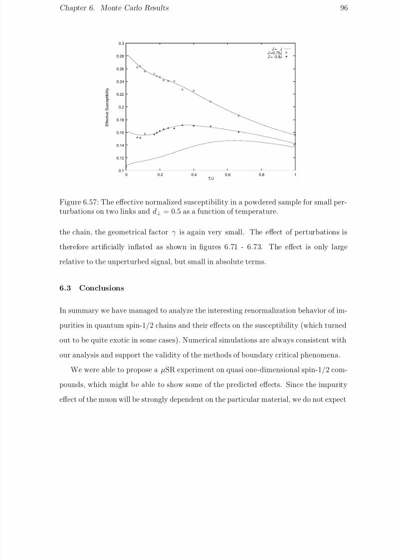
8/3/2019 Sebastian Eggert- Impurity Effects in Antiferromagnetic Quantum Spin-1/2 Chains
http://slidepdf.com/reader/full/sebastian-eggert-impurity-effects-in-antiferromagnetic-quantum-spin-12-chains 111/132
Chapter 6. Monte Carlo Results 96
0.1
0.12
0.14
0.16
0.18
0.2
0.22
0.24
0.26
0.28
0.3
0 0.2 0.4 0.6 0.8 1
E f f e c t i v e S u s c e p t i b i l i t y
T/J
J’= JJ’=0.75JJ’= 0.9J
Figure 6.57: The effective normalized susceptibility in a powdered sample for small per-turbations on two links and d⊥ = 0.5 as a function of temperature.
the chain, the geometrical factor γ is again very small. The effect of perturbations is
therefore artificially inflated as shown in figures 6.71 - 6.73. The effect is only large
relative to the unperturbed signal, but small in absolute terms.
6.3 Conclusions
In summary we have managed to analyze the interesting renormalization behavior of im-
purities in quantum spin-1/2 chains and their effects on the susceptibility (which turned
out to be quite exotic in some cases). Numerical simulations are always consistent with
our analysis and support the validity of the methods of boundary critical phenomena.
We were able to propose a µSR experiment on quasi one-dimensional spin-1/2 com-
pounds, which might be able to show some of the predicted effects. Since the impurity
effect of the muon will be strongly dependent on the particular material, we do not expect

8/3/2019 Sebastian Eggert- Impurity Effects in Antiferromagnetic Quantum Spin-1/2 Chains
http://slidepdf.com/reader/full/sebastian-eggert-impurity-effects-in-antiferromagnetic-quantum-spin-12-chains 112/132
Chapter 6. Monte Carlo Results 97
0.1
0.11
0.12
0.13
0.14
0.15
0.16
0.17
0.18
0.19
0.2
0 0.2 0.4 0.6 0.8 1
E f f e c t i v e S u s c e p t i b i l i t y
T/J
J’= JJ’=0.75JJ’= 0.9J
Figure 6.58: The effective normalized susceptibility in a powdered sample for small per-turbations on two links and d⊥ = 1 as a function of temperature.
0
0.5
1
1.5
2
2.5
3
3.5
4
0 0.1 0.2 0.3 0.4 0.5 0.6 0.7 0.8 0.9 1
E f f e c t i v e S u s c e p t i b i l i t y
T/J
J’= 0.1JJ’=0.25JJ’= 0.5J
Figure 6.59: The effective normalized susceptibility in a powdered sample for strongperturbations on two links and d⊥ = 0.5 as a function of temperature.

8/3/2019 Sebastian Eggert- Impurity Effects in Antiferromagnetic Quantum Spin-1/2 Chains
http://slidepdf.com/reader/full/sebastian-eggert-impurity-effects-in-antiferromagnetic-quantum-spin-12-chains 113/132
Chapter 6. Monte Carlo Results 98
0
0.5
1
1.5
2
2.5
0 0.2 0.4 0.6 0.8 1
E f f e c t i v e S u s c e p t i b i l i t y
T/J
J’= 0.1JJ’=0.25JJ’= 0.5J
Figure 6.60: The effective normalized susceptibility in a powdered sample for strongperturbations on two links and d⊥ = 1 as a function of temperature.
-0.1
-0.05
0
0.05
0.1
0.15
0 0.2 0.4 0.6 0.8 1
E f f e c t i v e S u s c e p t i b i l i t y
T/J
J’= JJ’=1.25J
J’= 2J
Figure 6.61: The effective normalized susceptibility in a powdered sample for twostrengthened links and d⊥ = 0.5 as a function of temperature.

8/3/2019 Sebastian Eggert- Impurity Effects in Antiferromagnetic Quantum Spin-1/2 Chains
http://slidepdf.com/reader/full/sebastian-eggert-impurity-effects-in-antiferromagnetic-quantum-spin-12-chains 114/132
Chapter 6. Monte Carlo Results 99
0.02
0.04
0.06
0.08
0.1
0.12
0.14
0.16
0 0.2 0.4 0.6 0.8 1
E f f e c t i v e S u s c e p t i b i l i t y
T/J
J’= JJ’=1.25J
J’= 2J
Figure 6.62: The effective normalized susceptibility in a powdered sample for twostrengthened links and d⊥ = 1 as a function of temperature.
0.1
0.15
0.2
0.25
0.3
0.35
0.4
0 0.2 0.4 0.6 0.8 1
E f f e c t i v e S u s c e p t i b i l i t y
T/J
J’= JJ’=0.75JJ’= 0.9J
Figure 6.63: The effective normalized susceptibility for an applied field perpendicular tothe chain, small perturbations on two links and d⊥ = 0.5 as a function of temperature.

8/3/2019 Sebastian Eggert- Impurity Effects in Antiferromagnetic Quantum Spin-1/2 Chains
http://slidepdf.com/reader/full/sebastian-eggert-impurity-effects-in-antiferromagnetic-quantum-spin-12-chains 115/132
Chapter 6. Monte Carlo Results 100
0.1
0.12
0.14
0.16
0.18
0.2
0.22
0.24
0.26
0.28
0.3
0 0.2 0.4 0.6 0.8 1
E f f e c t i v e S u s c e p t i b i l i t y
T/J
J’= JJ’=0.75JJ’= 0.9J
Figure 6.64: The effective normalized susceptibility for an applied field perpendicular tothe chain, small perturbations on two links and d⊥ = 1 as a function of temperature.
-0.2
-0.15
-0.1
-0.05
0
0.05
0.1
0.15
0 0.2 0.4 0.6 0.8 1
E f f e c t i v e S u s c e p t i b i l i t y
T/J
J’= JJ’=1.25J
J’= 2J
Figure 6.65: The effective normalized susceptibility for an applied field perpendicular tothe chain, two strengthened links and d⊥ = 0.5 as a function of temperature.

8/3/2019 Sebastian Eggert- Impurity Effects in Antiferromagnetic Quantum Spin-1/2 Chains
http://slidepdf.com/reader/full/sebastian-eggert-impurity-effects-in-antiferromagnetic-quantum-spin-12-chains 116/132
Chapter 6. Monte Carlo Results 101
-0.1
-0.05
0
0.05
0.1
0.15
0 0.2 0.4 0.6 0.8 1
E f f e c t i v e S u s c e p t i b i l i t y
T/J
J’= JJ’=1.25J
J’= 2J
Figure 6.66: The effective normalized susceptibility for an applied field perpendicular tothe chain, two strengthened links and d⊥ = 1 as a function of temperature.
0
0.5
1
1.5
2
2.5
3
3.5
4
4.5
5
0 0.1 0.2 0.3 0.4 0.5 0.6 0.7 0.8 0.9 1
E f f e c t i v e S u s c e p t i b i l i t y
T/J
J’= 0.1JJ’=0.25JJ’= 0.5J
Figure 6.67: The effective normalized susceptibility for an applied field perpendicular tothe chain, strong perturbations on two links and d⊥ = 0.5 as a function of temperature.

8/3/2019 Sebastian Eggert- Impurity Effects in Antiferromagnetic Quantum Spin-1/2 Chains
http://slidepdf.com/reader/full/sebastian-eggert-impurity-effects-in-antiferromagnetic-quantum-spin-12-chains 117/132
Chapter 6. Monte Carlo Results 102
0.1
0.15
0.2
0.25
0.3
0.35
0.4
0.45
0.5
0 0.2 0.4 0.6 0.8 1
E f f e c t i v e S u s c e p t i b i l i t y
T/J
J’= JJ’=0.75JJ’= 0.9J
Figure 6.68: The effective normalized susceptibility for an applied field parallel to thechain, small perturbations on two links and d⊥ = 0.5 as a function of temperature.
-0.35
-0.3
-0.25
-0.2
-0.15
-0.1
-0.05
0
0.05
0.1
0.15
0 0.2 0.4 0.6 0.8 1
E f f e c t i v e S u s c e p t i b i l i t y
T/J
J’= JJ’=1.25J
J’= 2J
Figure 6.69: The effective normalized susceptibility for an applied field parallel to thechain, two strengthened links and d⊥ = 0.5 as a function of temperature.

8/3/2019 Sebastian Eggert- Impurity Effects in Antiferromagnetic Quantum Spin-1/2 Chains
http://slidepdf.com/reader/full/sebastian-eggert-impurity-effects-in-antiferromagnetic-quantum-spin-12-chains 118/132
Chapter 6. Monte Carlo Results 103
0
1
2
3
4
5
6
7
0 0.1 0.2 0.3 0.4 0.5 0.6 0.7 0.8 0.9 1
E f f e c t i v e S u s c e p t i b i l i t y
T/J
J’= 0.1JJ’=0.25JJ’= 0.5J
Figure 6.70: The effective normalized susceptibility for an applied field parallel to thechain, strong perturbations on two links and d⊥ = 0.5 as a function of temperature.
0
0.2
0.4
0.6
0.8
1
1.2
1.4
1.6
1.8
0 0.2 0.4 0.6 0.8 1
E f f e c t i v e S u s c e p t i b i l i t y
T/J
J’= JJ’=0.75JJ’= 0.9J
Figure 6.71: The effective normalized susceptibility for an applied field parallel to thechain, small perturbations on two links and d⊥ = 1 as a function of temperature.

8/3/2019 Sebastian Eggert- Impurity Effects in Antiferromagnetic Quantum Spin-1/2 Chains
http://slidepdf.com/reader/full/sebastian-eggert-impurity-effects-in-antiferromagnetic-quantum-spin-12-chains 119/132
Chapter 6. Monte Carlo Results 104
-2
-1.5
-1
-0.5
0
0.5
0 0.2 0.4 0.6 0.8 1
E f f e c t i v e S u s c e p t i b i l i t y
T/J
J’= JJ’=1.25J
J’= 2J
Figure 6.72: The effective normalized susceptibility for an applied field parallel to thechain, two strengthened links and d⊥ = 1 as a function of temperature.
0
5
10
15
20
25
30
0 0.2 0.4 0.6 0.8 1
E f f e c t i v e S u s c e p t i b i l i t y
T/J
J’= 0.1JJ’=0.25JJ’= 0.5J
Figure 6.73: The effective normalized susceptibility for an applied field parallel to thechain, small perturbations on two links and d⊥ = 1 as a function of temperature.

8/3/2019 Sebastian Eggert- Impurity Effects in Antiferromagnetic Quantum Spin-1/2 Chains
http://slidepdf.com/reader/full/sebastian-eggert-impurity-effects-in-antiferromagnetic-quantum-spin-12-chains 120/132
Chapter 6. Monte Carlo Results 105
that the numerical simulations of our generic models will be able to describe the expected
signal in full detail. However, we are confident that our Monte Carlo data provides a
rough quantitative estimate of the effects and describes the generic renormalization be-
havior, which seems to depend only on the symmetry properties of the perturbation (e.g.
the shift of the maximum and the increase of the signal can most likely be observed for
most any link symmetric weakening of links in the chain.) The Monte Carlo simulations
can be extended for any material once the location of the muon and its effect on the
chain have been estimated.
The main conclusion which can be drawn from the field theory analysis as well as
from the numerical simulations is the fact that impurities have a surprisingly large effect
on the susceptibility in these one-dimensional systems. The impurity effects on the
measured Knight shift for a muon in the chain are of the same order of magnitude as
the unperturbed susceptibility and may even dominate the signal. On the other hand, in
µSR experiments on higher dimensional magnetic compounds the impurity effect of the
muon is neglected in most cases.

8/3/2019 Sebastian Eggert- Impurity Effects in Antiferromagnetic Quantum Spin-1/2 Chains
http://slidepdf.com/reader/full/sebastian-eggert-impurity-effects-in-antiferromagnetic-quantum-spin-12-chains 121/132
Appendix A
Field Theory Formulas
In this appendix we would like to give a short summary of the central (1+1) dimensional
field theory formulas, which have been used in this thesis. These formulas are explained
and derived in references [18] and [40] in a pedagogical way. Reference [10] may also be
of some use. We will not attempt to reproduce the derivation in a compressed form, since
it is not possible without assuming a common background.
Green’s functions of left- and right-movers always separate into a product, unless
they are related by a boundary condition. We can therefore look at the expressions for
left- and right-movers separately and simply add the scaling dimensions d = dL + dR.
The two-point boson Green’s function can be calculated directly from the infinite length
mode expansion:
< φL(x, t)φL(0, 0) > = − 1
4πln i(x + vt) + const.
< φR(x, t)φR(0, 0) > = −1
4π ln i(x − vt) + const., (A.102)
where the constant is cutoff dependent. The Green’s function for the boson derivative is
given by the second derivative of equation (A.102)
∂φL
∂x(x, t)
∂φL
∂x(0, 0)
= − 1
4π(x + vt)2∂φR
∂x(x, t)
∂φR
∂x(0, 0)
= − 1
4π(x − vt)2(A.103)
so that the usual fermion current scaling dimension d = 1 is recovered. Equation (A.102)
106

8/3/2019 Sebastian Eggert- Impurity Effects in Antiferromagnetic Quantum Spin-1/2 Chains
http://slidepdf.com/reader/full/sebastian-eggert-impurity-effects-in-antiferromagnetic-quantum-spin-12-chains 122/132
Appendix A. Field Theory Formulas 107
also implies a scaling dimension of dL = γ 2/8π for eiγφL , since
eiγφL(x,t)e−iγφL(0,0)
∝
: eiγ [φL(x,t)−φL(0,0)] :
eγ
2<φL(x,t)φL(0,0)>
∝ e− ln i(x+vt)γ 2/4π = −i
x + vt
γ 2/4π
(A.104)
which is in complete agreement with bosonization in equation (2.9) and fermionic Green’s
functions. This equation can be generalized to
< ei
jγ jφL(zi) >∝
j=k
−i
z j − zk
γ jγ k/8π
, (A.105)
where zi = xi + vti. This relation is useful for equation (3.35). We also see that single
powers of eiγφL have a vanishing expectation value.
From equation (2.10) it is clear that the commutator of the left- and right-movingbosons is i/4 which is essential for the bosonization formulas (2.9) to work. For fixed
boundary conditions the commutation relation is modified at the origin because left-
and right-movers are related there. It takes some careful analysis of the finite length
mode expansion in equation (3.48) to obtain the correct value of the commutator at
the boundary. This calculation has been done by Eugene Wong (unpublished), and the
results are
[φL, φR] = 0, x = y = 0
i2 , x = y = l
i4
, else (A.106)
Conformal transformations are represented by analytic functions in the complex plane
ω(z), and chiral primary operators OL are defined as operators which transform as
OL(z) →
dωdz
dL
OL(ω), (A.107)

8/3/2019 Sebastian Eggert- Impurity Effects in Antiferromagnetic Quantum Spin-1/2 Chains
http://slidepdf.com/reader/full/sebastian-eggert-impurity-effects-in-antiferromagnetic-quantum-spin-12-chains 123/132
Appendix A. Field Theory Formulas 108
where dL is the scaling dimension of OL. In this sense conformal transformations gener-
alize scale transformations, Lorentz transformations and translations all of which can be
represented by an analytic function ω(z) in the complex plane for (1+1) dimensions. One
application of equation (A.107) is the the transformation ω(z) = e2πz/vβ which gives the
well known result in equation (5.64) for finite temperature correlation functions. Note,
that ω is periodic in imaginary time with radius β .
Conformal invariance dictates a unique form for three-point Green’s functions of pri-
mary operators
OL
1 (z1)OL2 (z3)OL
3 (z3)
∝ (z1 − z2)−(d1+d2−d3)(z1 − z3)−(d1+d3−d2)(z2 − z3)−(d2+d3−d1)
(A.108)
where di, i = 1, 2, 3 are the scaling dimensions of the three primary operators OL
i andzi = xi + vti.

8/3/2019 Sebastian Eggert- Impurity Effects in Antiferromagnetic Quantum Spin-1/2 Chains
http://slidepdf.com/reader/full/sebastian-eggert-impurity-effects-in-antiferromagnetic-quantum-spin-12-chains 124/132
Appendix B
Exact Diagonalization Algorithm
The algorithm we used starts from a normalized initial trial vector Ψ1 and successively
minimizes the energy expectation value in each iteration step by forming the linear com-
bination Ψ2 = bΨ1 + H Ψ1. The explicit formulae are
b =1
2∆2(∆3 −
∆2
3 + 4∆2∆4), (B.109)
so that the normalized improved ground state is given by
Ψ2 =bΨ1 + H Ψ1
(b2 + 2b < H > + < H 2 >)1
2
. (B.110)
where
∆2 = < H 2 > − < H >2
∆3 = < H >< H 2 > − < H 3 >
∆4 = < H 2 >2
−< H >< H 3 > (B.111)
Here, we used the notation < H n > = < Ψ1 |H n| Ψ1 >. The new energy expectation
value is given by
< Ψ2 |H | Ψ2 > = < H > −
∆23 + 4∆2∆4
b2 + 2b < H > + < H 2 >(B.112)
The algorithm terminates when we are close enough to the ground state so that the
energy cannot be lowered much further. Clearly, all symmetries of Ψ1 are preserved in
each step, so the algorithm can be used to find ground states in different sectors of H ,
which are characterized by convenient quantum numbers.
109

8/3/2019 Sebastian Eggert- Impurity Effects in Antiferromagnetic Quantum Spin-1/2 Chains
http://slidepdf.com/reader/full/sebastian-eggert-impurity-effects-in-antiferromagnetic-quantum-spin-12-chains 125/132
Appendix B. Exact Diagonalization Algorithm 110
We decided to work in the orthonormal S z-basis because the next nearest neighbor
coupling requires excessive computations in the valence bond basis[41], which keeps track
of the total spin. The basis states can be represented by integer bit strings, and the
Hamiltonian was implemented as a procedure that manipulates and then stores the bit
strings and their coefficients as they are created. For numerical convenience we used
the Exchange Hamiltonian, which differs by a factor of two and a constant from the
Heisenberg Hamiltonian in equation (1.1) with J = J z. The various tricks to optimize
the algorithm include a hashing technique[15], extrapolation to the exact ground state,
and reusing previously created information on how to update basis states. The resulting
ground state can be used as an initial starting state for a similar Hamiltonian with only
slightly modified parameters. The extrapolation is based on the fact that the actual
ground state energy is approached exponentially and simply uses the last three iteration
values to find an improved result. This can give reliably at least two more digits accuracy.
In all problems the translational invariance is broken by the impurity. Taking into
account the limited remaining available symmetries of our problem, we can handle only
about 22 sites on a SUN workstation (about 8 sites less than what can be done for a
periodic chain in the valence bond basis). Some calculations were done on a NEC SX3/44
supercomputer because supercomputers generally allow for about four more sites. Work-
ing in the valence bond basis with s = 0 and using translational and parity invariance we
can find the exact ground state to 8 digits accuracy of a periodic chain of 24 sites in only
15 seconds CPU time on a NEC SX3/44 supercomputer. This needs to be compared
to 20 min CPU time on a SPARCstation2 when working in the S z-basis on the same
problem.

8/3/2019 Sebastian Eggert- Impurity Effects in Antiferromagnetic Quantum Spin-1/2 Chains
http://slidepdf.com/reader/full/sebastian-eggert-impurity-effects-in-antiferromagnetic-quantum-spin-12-chains 126/132
Appendix C
Monte Carlo Algorithm
The goal is to make predictions of measurements of physical quantities expressed in terms
of quantum mechanical operators at finite temperatures. The expectation value of any
operator A is given in terms of the partition function Z =
k < k|e−βH |k >:
< A > =
k < k |Ae−βH |k >
Z (C.113)
where the sum is over all basis states |k > of the system and β = 1/T . For example, the
local susceptibility at site i would be given by:
χi = β
k < k | j S z j S zi e−βH |k >
Z = β <
j
S z j S zi > (C.114)
To calculate these sums exactly, we would first need to diagonalize H in the Hilbert
space to express exp(−βH ) and then sum over all eigenstates. Since the dimension of
the Hilbert space grows exponentially with the system size l, the exact diagonalization of
H cannot be done for more than N ≈ 30 spins as indicated in appendix B. In addition
we would have to sum over all eigenvalues to get a finite temperature expression.
To get around this problem of large Hilbert spaces we use the quantum Monte Carlo
method. We first transform the expression in equation (C.113) so that the exponential of
the Hamiltonian can be evaluated approximately by use of the Trotter formula. We can
split the Hamiltonian (1.1) into two parts H = H e + H o, where the two parts involve only
the links S i ·
S i+1 with i even or odd, respectively. The two parts are easily diagonalized
separately, but they do not commute. Although exp(−βH ) = exp(−βH e) exp(−βH o),
111

8/3/2019 Sebastian Eggert- Impurity Effects in Antiferromagnetic Quantum Spin-1/2 Chains
http://slidepdf.com/reader/full/sebastian-eggert-impurity-effects-in-antiferromagnetic-quantum-spin-12-chains 127/132
Appendix C. Monte Carlo Algorithm 112
we can write an approximate (Trotter) formula for the expression in (C.113):
< k|Ae−βH |k > ≈ (C.115)
li
< k |Ae−2βH e/m|l1 >< l1|e−2βH o/m|l2 >< l2| ..... |lm−1 >< lm−1|e−2βH o/m|k >
This approximation becomes exact in the limit m → ∞. We have inserted m−1 complete
set of states |li > between each of the exponentials and we have to sum over all possible
combinations. While it is now relatively easy to compute the exponentials, we now have
the formidable task of summing over (2N )m possible configurations. Here we make use of
the principle of Monte Carlo integration: we statistically evaluate the sum by randomly
summing expression (C.115) over a lot of different configurations |li > and assume that
the average value will give us a good estimate of the complete sum.
This method is assisted by the fact that most configurations give a zero contribution
because the expectation values < li|e−βH |li+1 > are only non-zero for states that obey
certain selection rules. In fact we can evaluate the sums by going between allowed
configurations by using “moves” in configuration space which explicitly obey the selection
rules. By just using two different “moves” we can reach any allowed configuration, which
is sufficient to assure a complete sampling.
Furthermore, by assigning each “move” from an old configuration to a new one aprobability which is proportional to the change in the exponential
< newi|e−βH |newi+1 >
< oldi|e−βH |oldi+1 >
we automatically take care of evaluating the expression (C.115) without having to weigh
each contribution separately. This method is called importance sampling. The physical
idea is that the system spends most time in configurations for which the partition func-
tion Z is large. After a certain number of moves we can make a “measurement” of a
quantity by applying the corresponding operator A on the given configuration. Successive

8/3/2019 Sebastian Eggert- Impurity Effects in Antiferromagnetic Quantum Spin-1/2 Chains
http://slidepdf.com/reader/full/sebastian-eggert-impurity-effects-in-antiferromagnetic-quantum-spin-12-chains 128/132
Appendix C. Monte Carlo Algorithm 113
measurements may not be completely independent of each other unless a large number
of moves have been made. Just like in a physical system, the measurement of a quantity
A has a statistical distribution, and the mean would correspond to the expectation value
< A > in equation (C.113).
The only approximation we have made corresponds to equation (C.115), where a
larger m will yield better results. Fortunately, it is known[42] that the measurements
of < A > will have a leading correction of order 1/m2, so that we can extrapolate
analytically to the infinite m limit. This result follows directly from the accuracy of the
Trotter formula itself.
On the computer this method is implemented in a very straightforward way. As
indicated in equation (C.115) a complete configuration consists of m states, each of
which has N spins which can point up or down. A complete configuration is therefore
simply represented by an N × m array of boolean variables (“spins”). We select two
possible moves: local and global. The local move may flip 4 adjacent spins depending
on their configuration, and the global move may flip all spins at a given site, but for
all m states simultaneously. The probabilities of these moves are known for a given
temperature T = 1/β , and a good random number generator determines if a possible
move will be executed. To derive the detailed nature of the moves and probabilities it
takes some straightforward, but lengthy analysis of the physical system. This is omitted
here because it is rather technical and not important for the understanding of the method.
For more details see for example reference [42].
The update of the array is done in “sweeps” which consist of offering moves at all
possible locations in the array. The actual measurements of χi from equation (C.114)
take less time and are done after each sweep. Good results at lower temperatures require
larger arrays (generally 2m ≈ N > 10J/T is a good estimate). Typically the array has
dimensions of N = 48 − 128 by m = 24 − 64. Both m and N are even numbers, because

8/3/2019 Sebastian Eggert- Impurity Effects in Antiferromagnetic Quantum Spin-1/2 Chains
http://slidepdf.com/reader/full/sebastian-eggert-impurity-effects-in-antiferromagnetic-quantum-spin-12-chains 129/132
Appendix C. Monte Carlo Algorithm 114
periodic boundary conditions in the m direction are required. The number of offered
moves per sweep is roughly given by m × N .
Starting from any allowed configuration, a few thousand sweeps are done to bring the
system into equilibrium. To get one good average value we then did 2,000,000 sweeps
and measurements for a given array. For a choice of coupling and temperature, 3-5 of
those average values have to be taken at different values for m, so that a reasonable
extrapolation m → ∞ can be done. For one measurement point a total of roughly
3 × 10¹⁰ moves have to be checked and will be offered if possible. How many of these
possible moves will actually be executed strongly depends on the temperature. At higher
temperatures moves are more likely to be performed, which results in a faster update
and lower statistical errors.
It is obvious that the largest possible number of sweeps is desired, so that statistical
errors can be kept to a minimum. For this reason, I ported my program to the vector
supercomputer Fujitsu VPX240 of the HPC Centre, Calgary. The sweeps to update the
array take most of the computer time, and it is highly desirable to offer and perform
the moves in a vectorized way. This is not straight forward, because each move alters
the array and this may affect the outcome of a successive move. It took some extensive
analysis of the detailed nature of the moves to identify the dependencies, but finally it
was possible to separate the array into sublattices, so that all moves can be offered and
performed in vectorized loops.

8/3/2019 Sebastian Eggert- Impurity Effects in Antiferromagnetic Quantum Spin-1/2 Chains
http://slidepdf.com/reader/full/sebastian-eggert-impurity-effects-in-antiferromagnetic-quantum-spin-12-chains 130/132
Bibliography
[1] H. Bethe, Z. Physik, 71, 205 (1931)
[2] C.N. Yang, C.P. Yang, Phys. Rev. 50, 327 (1966).
[3] M. Takahashi, Prog. Theor. Phys. 46, 401 (1971); M. Takahashi, Phys. Rev. B43,5788 (1990).
[4] K. Hirikawa, Y. Kurogi, Prog. Theor. Phys. 46, 147 (1970).
[5] CPC refers to “dichlorobis(pyridine)copper(II)” which has been studied by W. Duffy,Jr., J.E. Venneman, D.L. Strandburg, P.M. Richards, Phys. Rev. B9, 2220 (1974).
[6] Y. Imry, P. Pincus, D. Scalapino, Phys. Rev. B11, 1978 (1975).
[7] C.A. Doty, D. Fisher, Phys. Rev. B45, 2167 (1992); D. Fisher, unpublished notes.
[8] For a summary of various applications of boundary critical phenomena and earlierreferences see I. Affleck, “Conformal Field Theory Approach to Quantum ImpurityProblems” preprint (1993), (Sissa preprint server number: cond-mat 9311054).
[9] S. Eggert, I. Affleck, Phys. Rev. B 46, 10866, (1992).
[10] For a review of the conformal field theory treatment of the spin-1/2 chain and earlierreferences see I. Affleck, Fields, Strings and Critical Phenomena (ed. E. Brezin andJ. Zinn-Justin North-Holland, Amsterdam, 1990), p.563.
[11] E. Lieb, T. Schultz, D. Mattis, Ann. Phys. (N.Y.) 16, 407 (1961).
[12] J. des Cloiseaux, M. Gaudin J. Math. Phys. 7, 1384 (1966); R.J. Baxter, Ann. Phys.(N.Y.) 70, 193 (1972).
[13] A. Luther, I. Peschel, Phys. Rev. B12, 3908 (1975).
[14] B.M. Coy, Phys. Rev. 173, 531 (1968).
[15] E.R. Gagliano, E.D. Moreo, A. Moreo, F.C. Alcarez, Phys. Ref. B34, 1677 (1986).
[16] S. Liang, Phys. Rev. Lett., 64, 1597 (1990).
[17] K. Wilson, Proceedings of the Midwest Conference on Theoretical Physics (NotreDame, April 1970), p.131.
115

8/3/2019 Sebastian Eggert- Impurity Effects in Antiferromagnetic Quantum Spin-1/2 Chains
http://slidepdf.com/reader/full/sebastian-eggert-impurity-effects-in-antiferromagnetic-quantum-spin-12-chains 131/132
Bibliography 116
[18] P. Ginsparg, Fields, Strings and Critical Phenomena (ed. E. Brezin and J. Zinn-Justin North-Holland, Amsterdam, 1990).
[19] I. Affleck, D. Gepner, H.J. Schulz, T. Ziman, J. Phys. A22, 511, (1989).
[20] F.D.M. Haldane, Phys. Rev. Lett. 60, 635 (1988).
[21] F.C. Alcarez, M.N. Barber, M.T. Batchelor, Phys. Rev. Lett. 58, 771 (1987); I.Affleck, J.B. Marston, J. Phys.C21, 2511 (1988).
[22] F.C. Alcarez, M. Baake, U. Grimm, V. Rittenberg, J. Phys. A21, L117 (1988).
[23] C.L. Kane, M.P.A. Fisher, Phys. Rev. Lett. 68, 1220 (1992).
[24] C.L. Kane, M.P.A. Fisher, Phys. Rev. B46, 15233, (1992).
[25] D. Clarke, T. Giamarchi, B. Shraiman, Phys. Rev. B48, 7070 (1993).
[26] P. Nozieres, A. Blandin, J. de Phys. (Paris), 41, 193 (1980).
[27] I. Affleck, A.W.W. Ludwig, Phys. Rev. Lett. 68, 1046 (1992).
[28] I. Affleck, A.W.W. Nucl. Phys. B360, 641 (1991).
[29] I. Affleck, Phys. Rev. Lett. 56, 2763 (1986).
[30] S. Eggert, I. Affleck, M. Takahashi, Phys. Rev. Lett. 73, 332 (1994).
[31] J.C. Bonner, M.E. Fisher, Phys. Rev. 135, A640 (1964).
[32] I. Affleck, Nucl. Phys. B336, 517 (1990).
[33] See, for example P. Nozieres, Proceedings of the 14th Int.’l Conf. on Low Temp. Phys.(ed. M. Krusius and M. Vuorio, North Holland, Amsterdam, 1974) V.5, p. 339. andreferences therein; N. Andrei, Phys. Rev. Lett. 45, 773 (1980); P.B. Wiegmann,JETP Lett. 31, 364 (1980); P.W. Anderson, J. Phys. C3, 2346 (1970); K.G. Wilson,Rev. Mod. Phys. 47, 773 (1975).
[34] N. Andrei, C. Destri, Phys. Rev. Lett. 52, 364 (1984); P.B. Wiegmann, A.M.Tsvelick, J. Phys. C18, 159 (1985).
[35] A.W.W. Ludwig, I. Affleck, Phys. Rev. Lett., 67, 3160 (1991).
[36] TRIUMF Research Proposal, “Quantum Impurities in One Dimensional Spin 1/2
Chains” (1994), Spokesperson: R. Kiefl, Group members: I. Affleck, J.H. Brewer,K. Chow, S. Dunsinger, S. Eggert, A. Keren, R.F. Kiefl, A. MacFarlane, J. Sonier,Y.J. Uemura.

8/3/2019 Sebastian Eggert- Impurity Effects in Antiferromagnetic Quantum Spin-1/2 Chains
http://slidepdf.com/reader/full/sebastian-eggert-impurity-effects-in-antiferromagnetic-quantum-spin-12-chains 132/132
Bibliography 117
[37] R.F. Kiefl, G.M. Luke, S.R. Kreitzman, M. Celio, R. Keitel, J.H. Brewer, D.R.Noakes, Y.J. Uemura, A.M. Portis, V. Jaccarino, Phys. Rev. B35, 2079 (1987).
[38] J.H. Brewer, S.R. Kreitzman, D.R. Noakes, E.J. Ansaldo, D.R. Harshman, R. Keitel,Phys. Rev. B33, 7813 (1986).
[39] M.F. Collins, V.K. Tondon, W.J.L. Buyers, Intern. J. Magnetism 4, 17 (1973).
[40] R. Shankar, Summer Course on Low-Dimensional Quantum Field Theories For Con-densed Matter Physicists, ICTP, Trieste, 24 August - 4 September 1992.
[41] For a review of the valence bond basis see: K. Chang, I. Affleck, G.W. Hayden, Z.G.Soos, J. Phys. 1, 153 (1989).
[42] M.Marcu, A. Wiesler, J.Phys.A 18, 2479 (1985).