Seasonality and the Valuation of Commodity Options

Janis Back

WHU – Otto Beisheim School of Management

Marcel Prokopczuk

ICMA Centre, Henley Business School, University of Reading

Markus Rudolf

WHU – Otto Beisheim School of Management

June 2010

ICMA Centre Discussion Papers in Finance DP2010-08

Copyright 2010 Back, Prokopczuk, Rudolf. All rights reserved.

ICMA Centre University of Reading Whiteknights PO Box 242 Reading RG6 6BA UK Tel: +44 (0)1183 787402 Fax: +44 (0)1189 314741 Web: www.icmacentre.ac.uk Director: Professor John Board, Chair in Finance The ICMA Centre is supported by the International Capital Market Association

Electronic copy available at: http://ssrn.com/abstract=1514803

Seasonality and the Valuation ofCommodity Options

Janis Back,∗ Marcel Prokopczuk,† and Markus Rudolf‡

First version: October 2009This version: March 2010

Abstract

Price movements in many commodity markets exhibit significant seasonalpatterns. In this paper, we study the effects of seasonal volatility on models’option pricing performance. In terms of options pricing, a deterministicseasonal component at the price level can be neglected. In contrast, this is nottrue for the seasonal pattern observed in the volatility of the commodity price.Analyzing an extensive sample of soybean and heating oil options, we find thatseasonality in volatility is an important aspect to consider when valuing thesecontracts. The inclusion of an appropriate seasonality adjustment significantlyreduces pricing errors and yields more improvement in valuation accuracy thanincreasing the number of stochastic factors.

JEL classification: G13

Keywords: Commodities, Seasonality, Options Pricing

∗Department of Finance, WHU - Otto Beisheim School of Management, D-56179 Vallendar,Germany. e-mail: janis.back@whu.edu. Telephone: +49-261-6509-397. Fax: +49-261-6509-399.

†ICMA Centre, Henley Business School, University of Reading, Reading, RG6 6BA, UnitedKingdom. e-mail: m.prokopczuk@icmacentre.ac.uk. Telephone: +44-118-378-4389. Fax: +44-118-931-4741.

‡Department of Finance, WHU - Otto Beisheim School of Management, D-56179 Vallendar,Germany. e-mail: markus.rudolf@whu.edu. Telephone: +49-261-6509-421. Fax: +49-261-6509-409.

Electronic copy available at: http://ssrn.com/abstract=1514803

I Introduction

Commodity options have a long history. One of the first usages was documented

by Aristotle, who reported in his book Politics (published 332 B.C.) a story about

the philosopher Thales, who was able to make good predictions on the next year’s

olive harvest, but did not have sufficient money to make direct use of his forecasts.

Therefore, Thales bought options on the usage of olive presses, which were available

for small premiums early in the year. When the harvest season arrived, and the

crop yield was, as expected by Thales, high, olive presses were in huge demand,

and he was able to sell his usage options for a small fortune.1 In contrast, modern

commodity options, as we know them today, are quite recent innovations. The first

commodity options traded at the Chicago Board of Trade (CBOT) were live cattle

and soybean contracts, both introduced in October 1984.2 As distinguished from

the ancient contracts, modern commodity options are generally not written on the

commodity itself, but on a future, as most of the trading takes place in the futures

market, ensuring liquidity of the underlying.

When considering the pricing of commodity options contracts, the special

features of these markets should be taken into account. One of the earliest,

and perhaps today’s most popular commodity options pricing formula among

practitioners, was derived by Black (1976). Black’s formula can basically be regarded

as a straight forward advancement of the well known Black and Scholes (1973) stock

options pricing formula, taking into account the fact that no initial outlay is needed

when entering a futures position. However, other stylized facts present in commodity

markets are not considered in Black’s approach. These issues have been addressed

in more recent research. Brennan (1991), Gibson and Schwartz (1990), Ross (1997),

and Schwartz (1997) point out that the dynamics of supply and demand result in a

mean-reverting behavior of commodity prices. Schwartz (1997) tests three different

model variants, incorporating mean-reversion (a one-, two-, and three-factor model),

1See Williams and Hoffman (2001), Chapter 1. The interested reader might also refer to thetranslated original text, e.g. Aristotle (1981), p. 88–90, where Aristotle refers to the strategy ofThales as a ‘money-spinning’ device.

2See the CME Group website: www.cmegroup.com.

2

in terms of their ability to price futures contracts on crude oil, copper, and gold.

All of these commodities belong to the part of the commodity universe not showing

seasonality in the price dynamics.

Seasonality can be considered as another stylized fact of many commodity

markets, distinguishing them from traditional financial assets. The seasonal

behavior of many commodity prices has been documented in numerous studies,

e.g. Fama and French (1987), and, thus, should be considered in a valuation

model. Sørensen (2002) considers the pricing of agricultural commodity futures

(corn, soybean, and wheat) by adding a deterministic seasonal price component to

the two-factor model of Schwartz and Smith (2000). Similarly, Lucia and Schwartz

(2002) and Manoliu and Tompaidis (2002) consider the electricity and natural gas

futures markets, respectively. Thus, the modeling of seasonality at the price level is

relatively well understood.

When it comes to options pricing, price level seasonality is, however, of no

importance. In a standard setting, the deterministic component of the price process

does not enter the options valuation formula.3 However, as noted by Choi and

Longstaff (1985), there exists a second type of seasonality which can have a great

influence on the value of a commodity option. As the degree of price uncertainty

changes through the year, the standard deviation, i.e. the volatility of a commodity

futures’ return, shows strong seasonal patterns. A good example is provided by

most agricultural markets, where the harvesting cycles determine the supply of

goods. Shortly before the harvest, the price uncertainty is higher than after the

harvest when crop yields are known to the market participants resulting in a seasonal

pattern in volatility in addition to the price level seasonality.

Surprisingly, the impact of seasonal volatility on commodity options valuation

3Intuitively, this can be seen by the fact that the deterministic price seasonality only affectsthe drift of the underlying. As the risk-free hedge portfolio must earn the risk-free rate, the priceseasonality cannot have any influence on the option price. More formally, this argument can be seenin the model description in Section III. One should note, however, that a predictable componentin the price process might have an influence on the estimation of the model parameters. If oneestimates the volatility using a historical time series of asset prices, one must clearly account forseasonal price variations as changes in the mean return affect the variance. As we estimate ourmodel implicitly using option prices, this problem does not arise. See also Lo and Wang (1995) onthis issue.

3

has attracted very little academic attention. Due to the lack of available options

data, Choi and Longstaff (1985) do not conduct any empirical study. Geman and

Nguyen (2005) and Richter and Sørensen (2002) consider the soybean market and

acknowledge the time-varying volatility by including a deterministic component in

their model, but do not study the impact on the models’ options pricing performance.

We contribute to the literature by filling this gap. Two commodity pricing

models, a one-factor and a two-factor model, are extended by allowing for seasonal

changes of volatility throughout the calendar year. These models are estimated using

an extensive sample of options prices for two different commodity markets. First,

we consider soybean options traded at the CBOT. Being the biggest agricultural

derivatives market, soybean contracts provide a prominent example of a commodity

with seasonality effects mainly induced from the supply side of the market. Second,

we study the impact of seasonalities on heating oil options traded at the New York

Mercantile Exchange (NYMEX). In contrast to the soybean market, the seasonality

in this market is mainly driven by the demand side. The considered options pricing

models are calibrated on a daily basis and then tested with respect to their in- and

out-of-sample pricing performance. Our results show that the pricing performance

can be greatly improved by including seasonality components in the volatility. This

demonstrates that considering the seasonality of volatility is of great importance

when dealing with options or option-like products in seasonally behaving commodity

markets.

The remainder of this paper is organized as follows. Section II provides an

overview of seasonality in commodity markets in general and the two considered

markets in specific. In Section III, we describe the considered model dynamics and

provide futures and options valuation formulas. Section IV describes the sample of

options data and the estimation procedure employed, while the empirical results of

our study are presented in Section V, and Section VI contains concluding remarks.

4

II Empirical Evidence on Seasonality in

Commodity Markets

Hylleberg (1992) defines seasonality as ”... the systematic, although not necessarily

regular, intra-year movement caused by the changes of the weather, the calendar, and

timing of decisions, directly or indirectly through the production and consumption

decisions made by agents of the economy. These decisions are influenced by

endowments, the expectations and preferences of the agents, and the production

techniques available in the economy.”

Following this definition, agricultural commodity markets clearly show seasonal

patterns induced by the supply side mainly due to harvesting cycles, the perishability

of agricultural goods, and the effects of weather. In contrast, many energy

commodity markets show seasonal patterns induced from the demand side, which

are due to regular climatic changes as well as regular calendar patterns, such as

holidays.4 Furthermore, inventories of these commodity markets undergo a seasonal

pattern. Thus, the presence of seasonality in commodity markets is also predicted by

the theory of storage (Kaldor (1939), Working (1949), Brennan (1958), and Telser

(1958)), which states that the convenience yield and, thus, the commodity price are

negatively related to the level of inventory.

In this paper, we consider two commodity markets: soybeans and heating oil.

The soybean market is the largest agricultural commodity market in the world,

whereas heating oil is, together with gasoline, the most important refined oil product

market.5

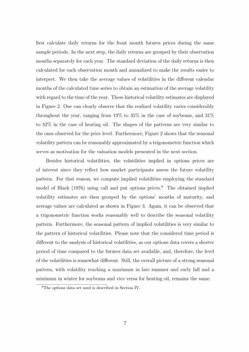
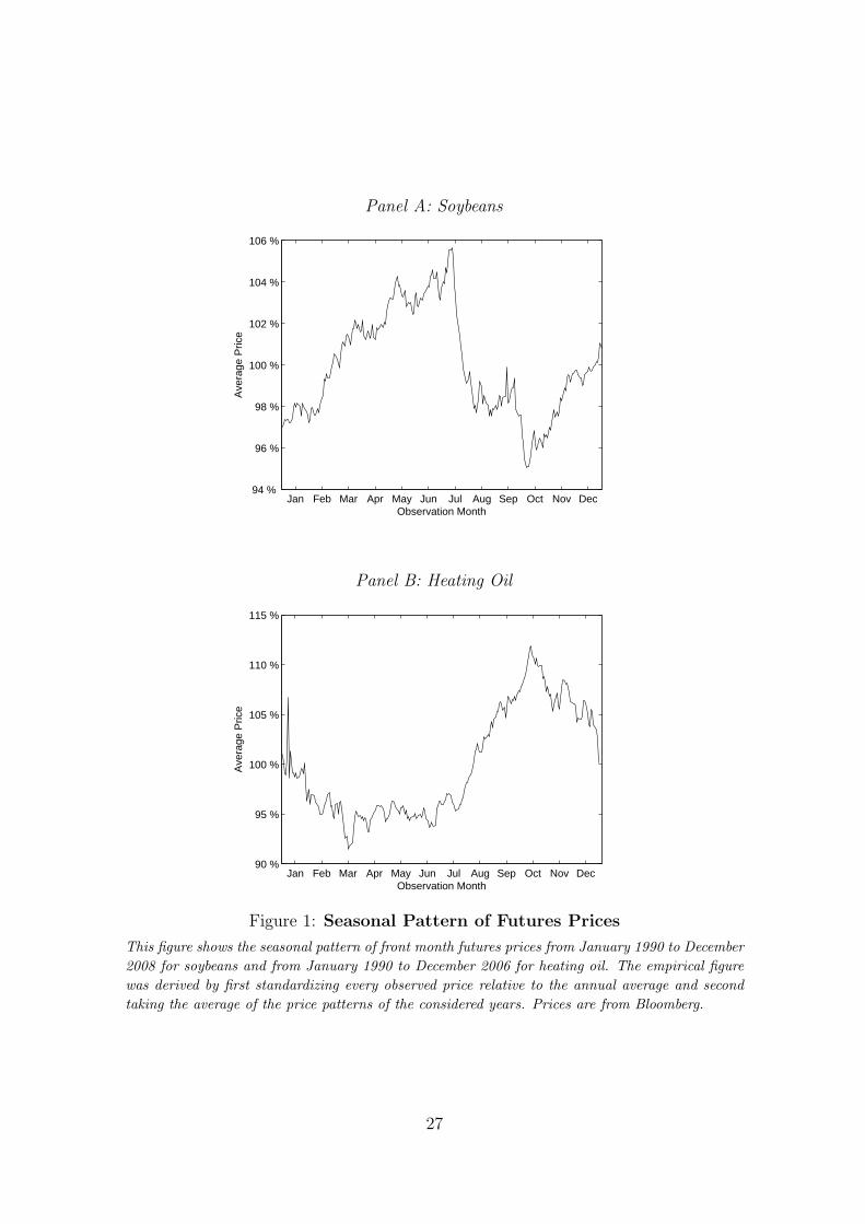
Although not the main focus of this paper, we first provide empirical evidence

on seasonal patterns at the price level to draw a complete picture with respect to

seasonality in the two considered markets. In order to illustrate the seasonal pattern

4In the case of electricity markets, varying demand levels induce regular intra-day and intra-weekprice patterns in addition to a calendar year effect as shown by ? and Lucia and Schwartz (2002),respectively.

5Details on these markets can be found in Geman (2005). The seasonal behavior of prices isdocumented by Milonas (1991), Frechette (1997) and Geman and Nguyen (2005) for the soybeanmarket, and Girma and Paulson (1998) and Borovkova and Geman (2006) for the heating oilmarket.

5

at the price level, we consider front month futures prices as an approximation of spot

prices. We standardize each daily price observation relative to the annual average.

Thereby, we obtain a price series describing the price pattern for each year considered

in our sample: January 1990 to December 2008 for the soybean futures, and January

1990 to December 2006 for the heating oil futures. In the next step, we calculate

average values of the annual patterns to derive the historical seasonal pattern of

the two considered commodities. Following the economic rationales outlined above,

we expect soybean prices to increase before the harvests in South America and the

United States, which take place during spring and summer.6 In the case of heating

oil, we expect the price to increase during the winter months when demand is higher

relative to the summer. These expected price patterns can be observed in Figure 1,

which displays the estimated seasonal price paths.

As discussed in the introduction, this paper focuses on a second type of

seasonality present in the price dynamics of commodity markets. According to

Anderson (1985), the volatility of commodity futures prices will be high during

periods when new information enters the market and significant amounts of supply or

demand uncertainty are resolved.7 For heating oil, this is the case during the winter

months, while in agricultural markets, this is true shortly before the harvesting

period. Information regarding the subsequent harvest becomes available during this

time, causing a higher fluctuation in prices, while a minimum is typically reached

during the winter months. These effects have been documented empirically for

various commodity markets.8

To analyze seasonality in volatility in the soybean and heating oil markets, we

calculate two different types of volatility: historical and option implied volatility.

To obtain historical (realized) volatilities for the two considered commodities, we

6South America, in particular Argentina and Brazil, and the United States are the world’sbiggest producers of soybeans.

7Note that there exists a second effect on volatility which is usually referred to as the Samuelsoneffect because it was first introduced by Samuelson (1965). This effect describes the empiricalfact that the volatility of futures increases as maturity approaches, which can be explained bydecreasing supplier flexibility. The Samuelson effect is implicitly accounted for by the commoditypricing models considered in this paper.

8See Anderson (1985), Choi and Longstaff (1985), Khoury and Yourougou (1993), Suenagaet al. (2008), and Karali and Thurman (2009) on seasonality in the volatility of commodity prices.

6

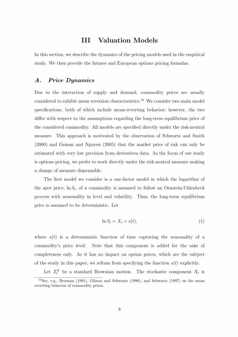
first calculate daily returns for the front month futures prices during the same

sample periods. In the next step, the daily returns are grouped by their observation

months separately for each year. The standard deviation of the daily returns is then

calculated for each observation month and annualized to make the results easier to

interpret. We then take the average values of volatilities in the different calendar

months of the calculated time series to obtain an estimation of the average volatility

with regard to the time of the year. These historical volatility estimates are displayed

in Figure 2. One can clearly observe that the realized volatility varies considerably

throughout the year, ranging from 19% to 35% in the case of soybeans, and 31%

to 82% in the case of heating oil. The shapes of the patterns are very similar to

the ones observed for the price level. Furthermore, Figure 2 shows that the seasonal

volatility pattern can be reasonably approximated by a trigonometric function which

serves as motivation for the valuation models presented in the next section.

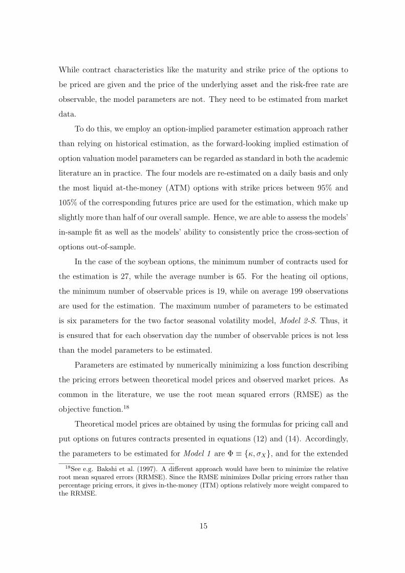
Besides historical volatilities, the volatilities implied in options prices are

of interest since they reflect how market participants assess the future volatility

pattern. For that reason, we compute implied volatilities employing the standard

model of Black (1976) using call and put options prices.9 The obtained implied

volatility estimates are then grouped by the options’ months of maturity, and

average values are calculated as shown in Figure 3. Again, it can be observed that

a trigonometric function works reasonably well to describe the seasonal volatility

pattern. Furthermore, the seasonal pattern of implied volatilities is very similar to

the pattern of historical volatilities. Please note that the considered time period is

different to the analysis of historical volatilities, as our options data covers a shorter

period of time compared to the futures data set available, and, therefore, the level

of the volatilities is somewhat different. Still, the overall picture of a strong seasonal

pattern, with volatility reaching a maximum in late summer and early fall and a

minimum in winter for soybeans and vice versa for heating oil, remains the same.

9The options data set used is described in Section IV.

7

III Valuation Models

In this section, we describe the dynamics of the pricing models used in the empirical

study. We then provide the futures and European options pricing formulas.

A. Price Dynamics

Due to the interaction of supply and demand, commodity prices are usually

considered to exhibit mean reversion characteristics.10 We consider two main model

specifications, both of which include mean-reverting behavior; however, the two

differ with respect to the assumptions regarding the long-term equilibrium price of

the considered commodity. All models are specified directly under the risk-neutral

measure. This approach is motivated by the observation of Schwartz and Smith

(2000) and Geman and Nguyen (2005) that the market price of risk can only be

estimated with very low precision from derivatives data. As the focus of our study

is options pricing, we prefer to work directly under the risk-neutral measure making

a change of measure dispensable.

The first model we consider is a one-factor model in which the logarithm of

the spot price, ln St, of a commodity is assumed to follow an Ornstein-Uhlenbeck

process with seasonality in level and volatility. Thus, the long-term equilibrium

price is assumed to be deterministic. Let

ln St = Xt + s(t), (1)

where s(t) is a deterministic function of time capturing the seasonality of a

commodity’s price level. Note that this component is added for the sake of

completeness only. As it has no impact on option prices, which are the subject

of the study in this paper, we refrain from specifying the function s(t) explicitly.

Let ZXt be a standard Brownian motion. The stochastic component Xt is

10See, e.g., Brennan (1991), Gibson and Schwartz (1990), and Schwartz (1997) on the meanreverting behavior of commodity prices.

8

assumed to follow the dynamics

dXt = κ(µ−Xt)dt + σXeϕ(t)dZXt , (2)

with κ > 0 denoting the degree of mean-reversion towards the long run mean µ of

the process. The volatility of the process is characterized by σX and the function

ϕ(t), which describes the seasonal behavior of the asset’s volatility. In contrast to

s(t), ϕ(t) impacts the price of an option by directly affecting the underlying asset’s

volatility. Considering the empirical volatility patterns in Figures 2 and 3, we follow

Geman and Nguyen (2005) and specify the function ϕ(t) as

ϕ(t) = θ sin(2π(t + ζ)) (3)

with θ ≥ 0 and ζ ∈ [−0.5, 0.5] in order to ensure the parameters’ uniqueness. We

refer to this model as Model 1-S throughout the rest of the paper, indicating it as

a one-factor model with seasonal volatility.

The proposed one-factor model is closely linked to existing commodity pricing

models. By setting ϕ(t) = 0 and s(t) = 0, the model nests the one-factor model

proposed by Schwartz (1997).11 Thus, the model of Schwartz (1997) serves as a

natural benchmark and will be referred to as Model 1.12

In the second model considered, the assumption regarding the long-term

equilibrium price level is changed. Following the ideas presented by Schwartz

and Smith (2000), a second latent risk factor is added, representing the fact that

uncertainty about the long-term equilibrium price exists in the economy. The

following model will be refered to as Model 2-S, i.e. a two-factor model with seasonal

volatility. Let

ln St = Xt + Yt + s(t), (4)

11Note that Schwartz (1997) also considers two- and three-factor models in his study.12The proposed model can also be considered as a simpler version of the model considered by

Geman and Nguyen (2005), who studied the influence of inventory levels on the pricing of futurescontracts. As our main purpose is to investigate the benefits of modeling seasonality of volatility inthe context of empirical option pricing, we keep the model parsimonious to enhance implementationand interpretation.

9

with

dXt = µdt + σXeϕ(t)dZXt , (5)

dYt = −κYtdt + σY dZYt , (6)

where s(t) is again a deterministic function of time capturing seasonality effects

at the price level. The first stochastic component Xt describes the non-stationary

long-term equilibrium price process. The parameter µ captures the drift and σX

together with the deterministic function ϕ(t) capture the volatility of the process,

respectively. As for the one factor model, ϕ(t) governs the seasonality of volatility

and is again assumed to be described by (3). The zero mean Ornstein-Uhlenbeck

process Yt captures short-term deviations from the long-term equilibrium. The

parameter κ > 0 governs the speed of mean reversion, while σY governs the volatility

of the process. ZXt and ZY

t are standard Brownian motions with instantaneous

correlation ρ.

Note that for ϕ(t) = 0 and specifying s(t) accordingly, the model is identical

to the model proposed by Sørensen (2002). When also imposing s(t) = 0, one

obtains the well-known two-factor model of Schwartz and Smith (2000), which we

call Model 2 throughout the paper. This model has been studied extensively and,

thus, provides an ideal basis to build on our empirical analysis.13

One might argue that more complex pricing models exist compared to the ones

we use in this study, and theses models might include jumps, stochastic volatility,

or regime switching. However, as our main focus is on the influence of the impact of

deterministic changes of volatility on the pricing of options, we decided to employ

well established and understood models as benchmarks for our empirical study.

13Note that, although not labeling one of the factors as convenience yield, Schwartz and Smith(2000) showed that their latent factor approach is equivalent to the two-factor model of Gibsonand Schwartz (1990) which explicitly models the convenience yield. As the latent factor model ofSchwartz and Smith (2000) is more convenient for estimation, it is usually preferred in empiricalstudies.

10

B. Valuation of Futures and Options

As the price dynamics are directly specified under the risk-neutral measure, the

value of a futures contract is equal to the expected spot price at the contract’s

maturity.14 Since all state variables are normally distributed, the spot price follows

a log-normal distribution. Thus, conditional on information available at time zero,

the futures price with maturity T at time zero, denoted by F0(T ), is given by

ln F0(T ) = ln E[ST ]

= E[ln(ST )] + 12Var[ln(ST )].

(7)

For the one-factor model, Model 1-S, the futures price is therefore given by15

ln F0(T ) = e−κT X0 + µ(1− e−κT ) + s(T )

+12σ2

X

T∫0

e2θ sin(2π(u+ζ))e−2κ(T−u) du.

(8)

Analogously, the futures price in the two-factor model, Model 2-S, can be obtained

as

ln F0(T ) = X0 + µT + Y0e−κT + s(T ) + 1

2σ2

X

T∫0

e2θ sin(2π(u+ζ)) du

+(1− e−2κT )σ2

Y

4κ+ σXσY ρ

T∫0

eθ sin(2π(u+ζ))e−κ(T−u) du.

(9)

Similarly, the value of a European option on a futures contract can be

immediately calculated as the expected pay-off discounted at the risk-free rate r.

Therefore, the price of a call option, with exercise price K and maturity t written on

a future with maturity T at time zero, is given by c0 = e−rtE0[max(Ft(T )−K, 0)].

As all state variables are normally distributed, the log futures price ln Ft(T ) is

also normally distributed. The variance σ2F (t, T ) of ln Ft(T ) for Model 1-S is given

14Precisely, this relationship only holds for forward contracts in general. If one additionallyassumes independence between the risk-free rate and the commodity spot price, the forward andfuture prices are equal. Please refer to Cox et al. (1981) on this issue. In the following, we assumethe risk-free rate to be constant.

15For more detailed information on the pricing formulas for futures and options presented in thissection, please refer to the appendix.

11

by

σ2F (t, T ) = σ2

X e−2κ(T−t)

t∫

0

e2θ sin(2π(u+ζ))e−2κ(t−u) du, (10)

and for Model 2-S by

σ2F (t, T ) = σ2

X

t∫0

e2θ sin(2π(u+ζ)) du +σ2

Y

2κe−2κ(T−t) (1− e−2κt)

+ 2σXσY ρ e−κ(T−t)t∫

0

eθ sin(2π(u+ζ)) e−κ(t−u) du.

(11)

Thus, Ft(T ) follows a log-normal distribution and European option pricing formulas

can be obtained by following the arguments provided in Black (1976). Therefore,

the price of a European call option is given by

c0 = e−rt ·(F0(T )N(ε)−KN(ε− σF (t, T ))

), (12)

where N denotes the cumulative distribution function of the standard normal

distribution and ε is defined as

ε =ln(F0(T )/K) + 1

2σ2

F (t, T )

σF (t, T ). (13)

The formula of a European put can be derived accordingly and is given by

p0 = e−rt ·(KN(−ε + σF (t, T ))− F0(T )N(−ε)

). (14)

Note that, by the inclusion of seasonal volatility, the resulting pricing formulas are

only semi-analytical, i.e. the remaining integral has to be computed numerically.

IV Data Description and Estimation Procedure

A. Data

The data set used for our empirical study consists of daily prices of American style

options and corresponding futures contracts written on soybeans and heating oil. All

12

data are obtained from Bloomberg. In the case of soybeans, the data set includes

prices for call and put options on futures traded at the CBOT maturing between

January 2005 and November 2010. CBOT soybean futures and options are available

for seven different maturity months: January, March, May, July, August, September,

and November. For the heating oil options, the data set includes prices for call and

put options traded at the NYMEX with maturity months between January 2005

and December 2007. Heating oil futures and options are available with maturities

in all twelve calendar months.

Several exclusion criteria were applied when constructing our data set. In order

to avoid liquidity related biases, we only consider options with strike prices between

90% and 110% of the underlying futures prices. Following Bakshi et al. (1997), we

furthermore only consider options with at least six days to maturity for the same

reason. Due to discreteness in the reported prices, we excluded options with values

of less than $ 0.50. Additionally, price observations allowing for immediate arbitrage

profits by exercising the American option are excluded from our sample.

Since we want to assess the effects of seasonal volatility, it is necessary to ensure

that the seasonal pattern over the course of the calendar year is reflected in our

data. Hence, prices for options maturing in the various contract months need to be

available. Taking this into account, the time periods for our empirical study extend

from July 29, 2004 through June 22, 2009 for the soybean options, and October 21,

2004 to December 26, 2006 for the heating oil options.

Tables 1 and 2 summarize the properties of our data set consisting of daily

put and call options prices. The data set covers a total of 156,129 observations

for the soybean options, and 202,603 observations for the heating oil options. The

considered observations consist of options within different moneyness and maturity

categories. When the price of the futures contract is between 90% and 95% of the

option’s strike price, call (put) options are considered as out-of-the-money (in-the-

money). Both call and put options are considered to be at-the-money when the

price of the futures contract is between 95% and 105% of the option’s strike price.

When the price of the futures contract is between 105% and 110% of the option’s

13

strike price, call (put) options are considered as in-the-money (out-of-the-money).

Options with less than 60 days to expiration are considered to be short-term, while

those with 60 to 180 days are medium-term and options with more than 180 days

to expiration are long-term contracts. Interest rates used in our empirical study are

the 3-month USD Libor rates published by the British Bankers’ Association.16

The closed or semi-closed form solutions presented for the different valuation

models in Section III are only available for European style options. However, all

options in our data set are American style contracts. To deal with this issue, we

follow the approach taken by Trolle and Schwartz (2008). Using the analytical

approximation of the early exercise premium developed by Barone-Adesi and Whaley

(1987), we transform each American option price into its European counterpart.

The approach of Barone-Adesi and Whaley (1987) relies on the constant

volatility Black (1976) framework. The seeming inconsistency of this approach with

the valuation models described above is remedied by the fact that each option is

transformed separately. Therefore, the price characteristics regarding the influence

of maturity, moneyness, volatility, and so on should be reflected in the transformed

prices as well.17

Furthermore, it should be noted that the early exercise feature is of minor

importance in our study. For the data set including soybean futures options, the

average correction for the early exercise feature is only 0.68% for both call and put

options. In the case of the options on heating oil futures, the average premium for

early exercise is estimated to be 0.38% for the call options and 0.36 % for the put

options.

B. Model Estimation

The four different valuation models presented in Section III are the subject of our

empirical analysis. In order to compare these model specifications with regard to

their ability to price commodity options, we need to specify the models’ parameters.

16The interest rate data are obtained from Thomson Financial Datastream.17See also Trolle and Schwartz (2008) for a discussion regarding the justification of this approach.

14

While contract characteristics like the maturity and strike price of the options to

be priced are given and the price of the underlying asset and the risk-free rate are

observable, the model parameters are not. They need to be estimated from market

data.

To do this, we employ an option-implied parameter estimation approach rather

than relying on historical estimation, as the forward-looking implied estimation of

option valuation model parameters can be regarded as standard in both the academic

literature an in practice. The four models are re-estimated on a daily basis and only

the most liquid at-the-money (ATM) options with strike prices between 95% and

105% of the corresponding futures price are used for the estimation, which make up

slightly more than half of our overall sample. Hence, we are able to assess the models’

in-sample fit as well as the models’ ability to consistently price the cross-section of

options out-of-sample.

In the case of the soybean options, the minimum number of contracts used for

the estimation is 27, while the average number is 65. For the heating oil options,

the minimum number of observable prices is 19, while on average 199 observations

are used for the estimation. The maximum number of parameters to be estimated

is six parameters for the two factor seasonal volatility model, Model 2-S. Thus, it

is ensured that for each observation day the number of observable prices is not less

than the model parameters to be estimated.

Parameters are estimated by numerically minimizing a loss function describing

the pricing errors between theoretical model prices and observed market prices. As

common in the literature, we use the root mean squared errors (RMSE) as the

objective function.18

Theoretical model prices are obtained by using the formulas for pricing call and

put options on futures contracts presented in equations (12) and (14). Accordingly,

the parameters to be estimated for Model 1 are Φ ≡ {κ, σX}, and for the extended

18See e.g. Bakshi et al. (1997). A different approach would have been to minimize the relativeroot mean squared errors (RRMSE). Since the RMSE minimizes Dollar pricing errors rather thanpercentage pricing errors, it gives in-the-money (ITM) options relatively more weight compared tothe RRMSE.

15

one-factor model, Model 1-S, Φ ≡ {κ, σX , θ, ζ} must be estimated. The standard

two-factor model, Model 2, requires the estimation of Φ ≡ {κ, σX , σY , ρ}, while the

parameters Φ ≡ {κ, σX , σY , ρ, θ, ζ} must be estimated for Model 2-S in order to

additionally take the seasonal pattern of the volatility into account. The procedure

to obtain the parameter estimates Φ∗t for every observation date t can be summarized

as follows:

Φ∗t = arg min

Φt

RMSEt(Φt) = arg minΦt

√√√√ 1

Nt

Nt∑i=1

(P̂t,i(Φt)− Pt,i)2. (15)

Thereby, Pt,i is the observed market price of option i out of Nt option prices used

for the estimation at time t and P̂t,i(Φt) is the theoretical model price based on a set

of parameters Φt. Parameters are not allowed to take values inconsistent with the

model frameworks. In detail, the following restrictions were applied: κ, σX , σY > 0

and ρ ∈ (−1, 1). Furthermore, the parameters governing the seasonal pattern of

volatility were restricted to ensure their uniqueness: θ ≥ 0 and ζ ∈ [−0.5, 0.5].19

V Empirical Model Comparison

In this section, we report the results of our empirical study. First, we briefly discuss

the implied parameter estimates, and then present the in-sample and out-of-sample

pricing results of the valuation models when both including seasonal volatility and

excluding it.

A. Estimated Parameters

The median and mean values of the daily re-estimated implied parameters for

the soybean and heating oil options are reported in Tables 3 and 4, respectively.

From the differences between mean and median values, it becomes abundantly clear

that the obtained parameter estimates are far from constant over time. However,

19For the numerical estimation of the parameters, ρ was limited to -0.999 and 0.999, and forκ, σX and σY the lower boundaries of 0.001 were assumed. Furthermore, 10,000 was used as anartificial upper boundary for the parameters in the numerical estimation procedure.

16

this observation is not particularly unique to our study. It is well-known in

the literature that the cross-sectional re-estimation of option pricing models often

yields fluctuating parameter estimates.20 Especially noteworthy is the case of the

two-factor models for soybean options. The parameters behave erratically over time,

giving the impression of overspecification in this particular case. More precisely, the

parameter κ determining the mean reversion speed of the second factor is estimated

to take extremely high values in many instances. This implies that, in these cases,

the influence of the second factor is negligible. Accordingly, the volatility of the

second factor and the correlation coefficient show unrealistic values in these instances

as well. In contrast, the parameter values for the soybean one-factor models and all

heating oil specifications are more stable and seem to be of reasonable size.

B. In-Sample Model Comparison

For each day, we calculate the model prices of each option given by the respective

valuation model and the implied parameter values and compare them with their

observed counterparts. It is worth noting that it is only a true in-sample test for

the at-the-money options, as only these contracts have been used for the parameter

estimation. For the in-the-money and out-of-the-money contracts one might speak

of an out-of-sample test, although not with respect to time, but cross-sectionally.

As the models without seasonal volatility are nested in their counterparts with

seasonal volatility, a higher number of parameters results in a better in-sample model

fit for the latter ones. In contrast, Model 1-S and Model 2 are not nested in each

other, and it will be interesting to see what in-sample gain in valuation precision can

be achieved by incorporating seasonal volatility versus a second stochastic factor.

Tables 5 and 6 display the in-sample results. We report the pricing errors

according to two different error metrics: the root mean squared error, RMSEt =√1

Nt

∑Nt

i=1(P̂t,i − Pt,i)2, and the relative root mean squared error, RRMSEt =√1

Nt

∑Nt

i=1(P̂t,i−Pt,i

Pt,i)2. Thereby, Pt,i is the observed market price of option i, P̂t,i is the

theoretical model price, and Nt is the number of observations at date t. As RMSE

20See, e.g., de Munnik and Schotman (1994).

17

was employed as the objective function in the estimation, it is most appropriate to

compare the in-sample fit with respect to this error metric.21 However, due to the

non-linear pay-off profile of options contracts, it is also interesting to see how this

relates to relative pricing errors. Furthermore, we present the results for the three

different maturity and moneyness brackets.

Comparing the models’ pricing fit between the soybean and heating oil options,

one can observe that the RMSE for the former is substantially higher in every

instance. However, this is a direct consequence of the different trading units and

price levels of the underlying assets.22 When considering RRMSE, the errors for

heating oil are still smaller than for the soybean options, but the difference is smaller

than when using RMSE.

The overall RMSE yield $ 4.50 for Model 1, $ 3.87 for Model 1-S, $ 4.29 for

Model 2, and $ 3.52 for Model 2-S for the soybean options. The corresponding

values for the heating oil options are $ 0.62, $ 0.48, $ 0.53, and $ 0.44. In both cases,

the models incorporating seasonal volatility outperform their counterparts, which

do not include this adjustment. Interestingly, Model 1-S, the one-factor model with

seasonality adjustment, yields lower errors than Model 2, the standard two-factor

model. Thus, allowing for seasonally varying volatility seems to be more important

than adding additional stochastic factors.

Considering the different moneyness categories, the ranking of the models

sustains. The out-of-the-money (OTM) and in-the-money (ITM) RMSE are slightly

higher than their at-the-money (ATM) counterparts for soybeans, while for heating

oil the ITM RMSE are slightly lower. Naturally, the RRMSE increases for OTM

and decreases for ITM options. In both markets, the RMSE is increasing along

the maturity brackets. This can be regarded as a direct consequence of the higher

average prices of longer maturity options in our sample as can be seen in Tables 1

and 2. The RRMSE do not show any clear pattern with respect to maturity.

21See Christoffersen and Jacobs (2004) on the selection of appropriate error metrics.22The average price of the front month futures during the considered time periods is $ 820.67 for

soybeans and $ 171.10 for heating oil.

18

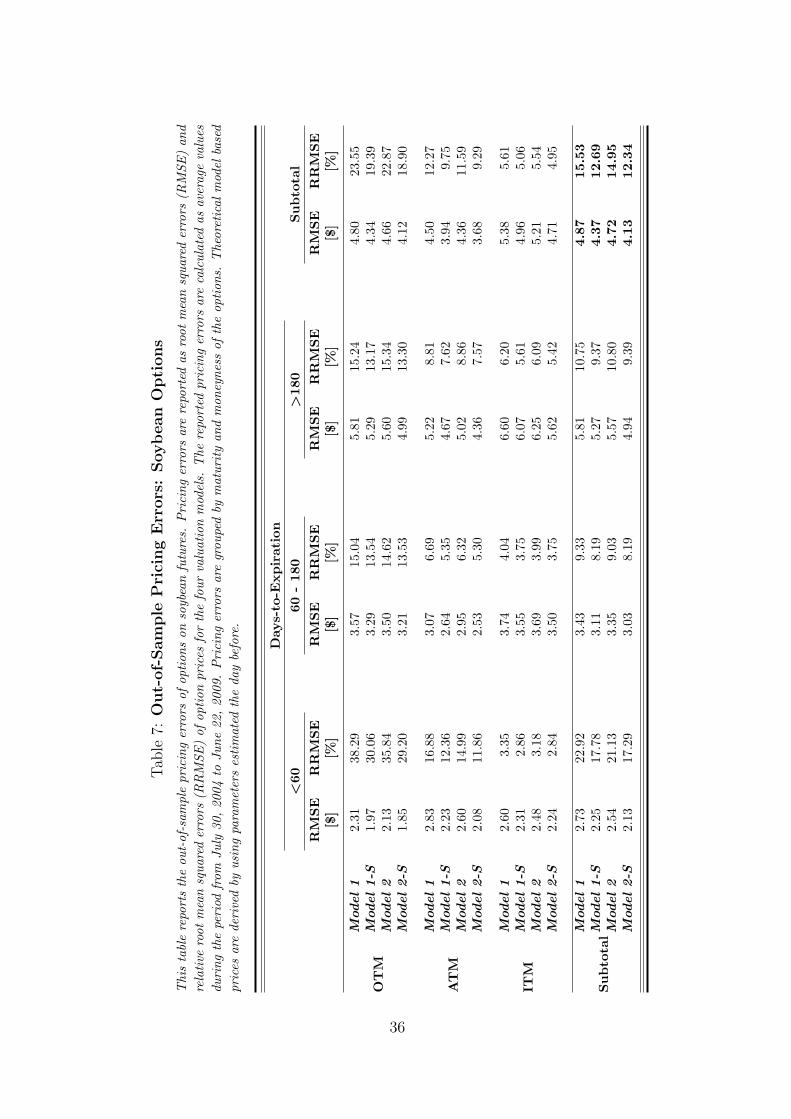
C. Out-of-Sample Model Comparison

The most conclusive way to compare different valuation models with respect to

their pricing accuracy is their out-of-sample performance. We thus proceed in

the following way: on each day, we compare the observed market prices with the

respective model prices using the parameters estimated on the previous day. In this

way, only information from the previous day enters the model evaluation. As for

the in-sample comparison, we report the results for RMSE and RRMSE, for OTM,

ATM, and ITM options, and for the three considered maturity brackets. The results

are provided in Table 7 for the soybean contracts, and in Table 8 for the heating oil

contracts.

The overall RMSE for the four models are $ 4.87, $ 4.37, $ 4.72, and $ 4.13 for

the soybean sample, and $ 0.66, $ 0.54, $ 0.58, and $ 0.51 for the heating oil sample.

Compared to their in-sample counterparts, one can observe that these errors are

about 5-15% higher, which is, of course, not surprising. More importantly, the

ranking of the four models remains identical to the in-sample case: the models

including seasonal volatility outperform their counterparts with constant volatility.

Again, the one-factor model including seasonality, Model 1-S, even beats Model 2,

the two-factor model without seasonality, in terms of RMSE and RRMSE.

Inspecting the results with respect to moneyness and maturity, it becomes

evident that the ranking of the models remains the same in almost all cases. Only in

the case of the relative errors (RRMSE), there are a few exceptions. For the soybean

options, the one-factor models perform slightly better than the two-factor models

for medium- and long-term contracts. Recalling the erratic parameter estimates of

the two-factor models, this result is not surprising. In our study, the second factor,

which mainly concerns the long-term behavior, does not seems to be necessary for

the soybean market. Nonetheless, the seasonal volatility model variants always beat

their constant volatility counterparts.

For the heating oil contracts, we can observe a few cases where Model 2

outperforms Model 1-S, e.g. for OTM and short-term options. These results

indicate that both a second stochastic factor and seasonal volatility are important

19

for increasing the pricing accuracy of the models. Combining these components in

Model 2-S yields the best out-of-sample performance in every case.

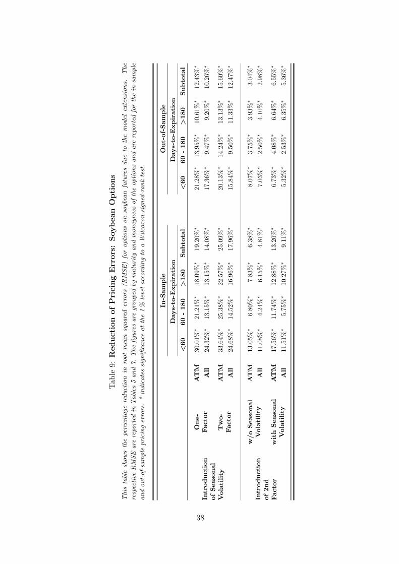
Lastly, to see whether the observed differences are statistically significant, we

perform Wilcoxon signed-rank tests to compare several model variants. Tables 9

(Soybeans) and 10 (Heating Oil) present the percentage reductions of the RMSE

when introducing a seasonal volatility component (upper parts) and when adding

a second stochastic factor (lower parts). The non-parametric Wilcoxon signed-rank

statistic tests whether the median of the differences is significantly different from

zero.

One can observe that incorporating seasonal volatility reduces the RMSE in

every instance, i.e. for both markets, both models, in-sample and out-of-sample, for

every maturity bracket, and for every moneyness category at a 1% significance level.

To keep the presentation manageable, we do not report the ITM and OTM results

separately; however, they do not deviate qualitatively from the results presented.

The overall pricing errors of the one- and two-factor models are reduced by 10.26%

and 12.47% for the soybean options, and by 18.37% and 11.95% for the heating

oil options in the out-of-sample test, respectively. The greatest improvements are

observed for short term heating oil contracts, with a maximal improvement of

37.96% for the ATM options and the one-factor model.

The introduction of the second stochastic factor also significantly improves the

pricing accuracy. The only exception is provided by the out-of-sample results in

the soybean case, where the observed improvements are smaller and, although

statistically significant, economically less important. This result, however, is

perfectly in line with our previous circumstantial evidence for overspecification.

Overall, our empirical findings provide clear evidence for the benefits of

valuation models including a seasonal adjustment to the volatility specification when

considering the pricing of soybean and heating oil futures options. The inclusion of

such a component, which is very simple from the modeling point of view, greatly

improves in-sample and, most importantly, out-of-sample pricing accuracy.

20

VI Conclusion

In this paper, we studied the impacts of seasonally fluctuating volatility in

commodity markets on the pricing of options. These seasonal effects are well-known

in the literature, but their impact on commodity options pricing has never been

investigated. We extended two standard continuous time commodity derivatives

valuation models to incorporate seasonality in volatility. Using an extensive data

set of soybean and heating oil options, we compared the empirical options pricing

accuracy of these models with their constant volatility counterparts. The results

showed that incorporating the stylized fact of seasonally fluctuating volatility greatly

improves the options valuation performance of the models. This leads to the

conclusion that seasonality in volatility should be accounted for when dealing with

commodity options.

Future research could extend our results in various ways. As a next step, one

could analyze the importance of seasonality in a stochastic volatility setting. It is

not clear what fraction of the fluctuation in volatility can be captured by seasonality

and what fraction remains stochastic. With respect to the modeling of seasonality,

it might be worth investigating which parametric assumption performs best for

different markets. Compared to the trigonometric approach taken in this paper,

one might model this component in other ways, e.g. by using simple step functions,

allowing for more complex seasonality patterns while relying on a higher number of

parameters.

21

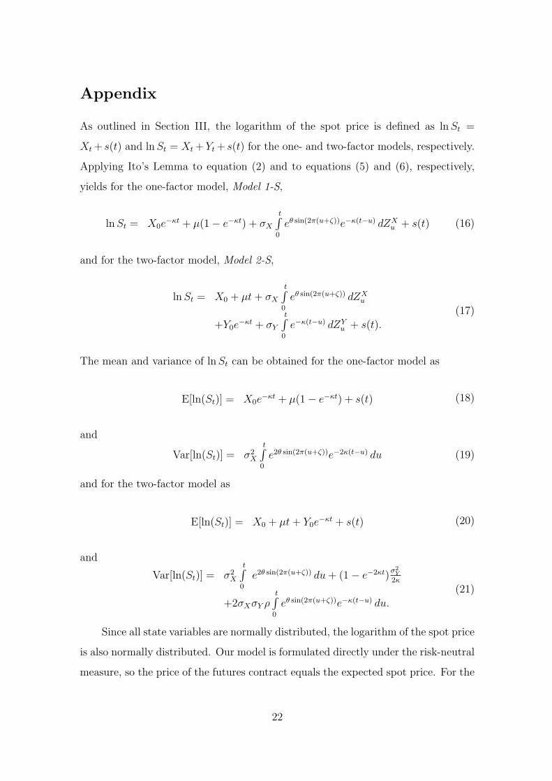
Appendix

As outlined in Section III, the logarithm of the spot price is defined as ln St =

Xt + s(t) and ln St = Xt +Yt + s(t) for the one- and two-factor models, respectively.

Applying Ito’s Lemma to equation (2) and to equations (5) and (6), respectively,

yields for the one-factor model, Model 1-S,

ln St = X0e−κt + µ(1− e−κt) + σX

t∫0

eθ sin(2π(u+ζ))e−κ(t−u) dZXu + s(t) (16)

and for the two-factor model, Model 2-S,

ln St = X0 + µt + σX

t∫0

eθ sin(2π(u+ζ)) dZXu

+Y0e−κt + σY

t∫0

e−κ(t−u) dZYu + s(t).

(17)

The mean and variance of ln St can be obtained for the one-factor model as

E[ln(St)] = X0e−κt + µ(1− e−κt) + s(t) (18)

and

Var[ln(St)] = σ2X

t∫0

e2θ sin(2π(u+ζ))e−2κ(t−u) du (19)

and for the two-factor model as

E[ln(St)] = X0 + µt + Y0e−κt + s(t) (20)

and

Var[ln(St)] = σ2X

t∫0

e2θ sin(2π(u+ζ)) du + (1− e−2κt)σ2

Y

2κ

+2σXσY ρt∫

0

eθ sin(2π(u+ζ))e−κ(t−u) du.

(21)

Since all state variables are normally distributed, the logarithm of the spot price

is also normally distributed. Our model is formulated directly under the risk-neutral

measure, so the price of the futures contract equals the expected spot price. For the

22

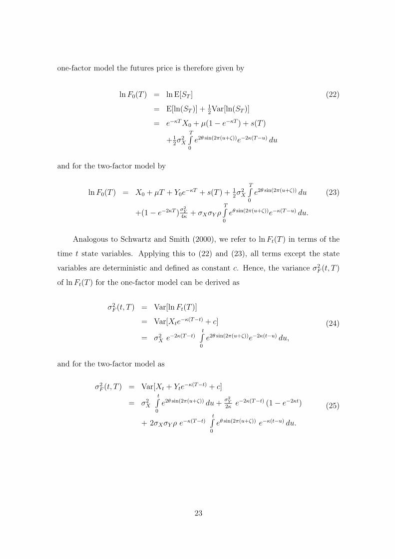
one-factor model the futures price is therefore given by

ln F0(T ) = ln E[ST ]

= E[ln(ST )] + 12Var[ln(ST )]

= e−κT X0 + µ(1− e−κT ) + s(T )

+12σ2

X

T∫0

e2θ sin(2π(u+ζ))e−2κ(T−u) du

(22)

and for the two-factor model by

ln F0(T ) = X0 + µT + Y0e−κT + s(T ) + 1

2σ2

X

T∫0

e2θ sin(2π(u+ζ)) du

+(1− e−2κT )σ2

Y

4κ+ σXσY ρ

T∫0

eθ sin(2π(u+ζ))e−κ(T−u) du.

(23)

Analogous to Schwartz and Smith (2000), we refer to ln Ft(T ) in terms of the

time t state variables. Applying this to (22) and (23), all terms except the state

variables are deterministic and defined as constant c. Hence, the variance σ2F (t, T )

of ln Ft(T ) for the one-factor model can be derived as

σ2F (t, T ) = Var[ln Ft(T )]

= Var[Xte−κ(T−t) + c]

= σ2X e−2κ(T−t)

t∫0

e2θ sin(2π(u+ζ))e−2κ(t−u) du,

(24)

and for the two-factor model as

σ2F (t, T ) = Var[Xt + Yte

−κ(T−t) + c]

= σ2X

t∫0

e2θ sin(2π(u+ζ)) du +σ2

Y

2κe−2κ(T−t) (1− e−2κt)

+ 2σXσY ρ e−κ(T−t)t∫

0

eθ sin(2π(u+ζ)) e−κ(t−u) du.

(25)

23

References

R. W. Anderson. Some determinants of the volatility of futures prices. Journal of

Futures Markets, 5:331–348, 1985.

Aristotle. The Politics - Tranlated by A. Sinclair. Prentice Hall, 1981.

G. Bakshi, C. Cao, and Z. Chen. Empirical performance of alternative option pricing

models. Journal of Finance, 52:2003–2049, 1997.

G. Barone-Adesi and R. E. Whaley. Efficient analytic approximation of American

option values. Journal of Finance, 42:301–320, 1987.

F. Black. The pricing of commodity contracts. Journal of Financial Economics, 3:

167–179, 1976.

F. Black and M. Scholes. The pricing of options and corporate liabilities. Journal

of Political Economy, 81:637–654, 1973.

S. Borovkova and H. Geman. Seasonal and stochastic effects in commodity forward

curves. Review of Derivatives Research, 9:167–186, 2006.

M. J. Brennan. The supply of storage. American Economic Review, 47:50–72, 1958.

M. J. Brennan. The price of convenience and the valuation of commodity contingent

claims. In D. Lund and B. Oksendal, editors, Stochastic Models and Option Values,

pages 33–71. Elsevier Science, 1991.

J.W. Choi and F.A. Longstaff. Pricing options on agricultural futures: An

application of the constant elasticity of variance option pricing model. Journal of

Futures Markets, 5:247–258, 1985.

P. Christoffersen and K. Jacobs. The importance of the loss function in option

valuation. Journal of Financial Economics, 72:291–318, 2004.

J. C. Cox, J. E. Jr. Ingersoll, and S. A. Ross. The relation between forward prices

and futures prices. Journal of Financial Economics, 9:321–346, 1981.

J.F.J. de Munnik and P.C. Schotman. Cross-sectional versus time series estimation

of term structure models: Empirical results for the Dutch bond market. Journal

of Banking and Finance, 18:997–1025, 1994.

E. F. Fama and K. R. French. Commodity futures prices: Some evidence on forecast

power, premiums, and the theory of storage. Journal of Business, 60:55–74, 1987.

24

D. L. Frechette. The dynamics of convenience and the Brazilian soybean boom.

American Journal of Agricultural Economics, 79:1108–1118, 1997.

H. Geman. Commodities and Commodity Derivatives. John Wiley & Sons Ltd,

Chichester, England, 2005.

H. Geman and V.-N. Nguyen. Soybean inventory and forward curve dynamics.

Management Science, 51:1076–1091, 2005.

R. Gibson and E. S. Schwartz. Stochastic convenience yield and the pricing of oil

contingent claims. Journal of Finance, 45:959–976, 1990.

P.B. Girma and A.S. Paulson. Seasonality in petroleum futures spreads. Journal of

Futures Markets, 18:581–598, 1998.

S. Hylleberg. Modelling Seasonality. Oxford University Press, 1. edition, 1992.

N. Kaldor. Speculation and economic stability. Review of Economic Studies, 7:1–27,

1939.

B. Karali and W.N. Thurman. Components of grain futures price volatility. Working

Paper, 2009.

N. Khoury and P. Yourougou. Determinants of agricultural futures price volatilities:

Evidence from Winnipeg Commodity Exchange. Journal of Futures Markets, 13:

345–356, 1993.

A. W. Lo and J. Wang. Implementing option pricing models when asset returns are

predictable. Journal of Finance, 50:87–129, 1995.

J. J. Lucia and E. S. Schwartz. Electricity prices and power derivatives: Evidence

from the nordic power exchange. Review of Derivatives Research, 5:5–50, 2002.

M. Manoliu and S. Tompaidis. Energy futures prices: term structure models with

Kalman filter estimation. Applied Mathematical Finance, 9:21–43, 2002.

N. T. Milonas. Measuring seasonalities in commodity markets and the half-month

effect. Journal of Futures Markets, 11:331–345, 1991.

M. Richter and C. Sørensen. Stochastic volatility and seasonality in commodity

futures and options: The case of soybeans. Working Paper, 2002.

S.A. Ross. Hedging long run commitments: Exercises in incomplete market pricing.

Banca Monte Economic Notes, 26:99–132, 1997.

25

P. A. Samuelson. Proof that properly anticipated prices fluctuate randomly.

Industrial Management Review, 6:41–49, 1965.

E. S. Schwartz. The stochastic behavior of commodity prices: Implications for

valuation and hedging. Journal of Finance, 52:923–973, 1997.

E. S. Schwartz and J. E. Smith. Short-term variations and long-term dynamics in

commodity prices. Management Science, 46:893–911, 2000.

C. Sørensen. Modeling seasonality in agricultural commodity futures. Journal of

Futures Markets, 22:393–426, 2002.

H. Suenaga, A. Smith, and J. Williams. Volatility dynamics of NYMEX natural gas

futures prices. Journal of Futures Markets, 28:438–463, 2008.

L. G. Telser. Futures trading and the storage of cotton and wheat. Journal of

Political Economy, 66:233–255, 1958.

A. B. Trolle and E. S. Schwartz. Unspanned stochastic volatility and the pricing of

commodity derivatives. Working Paper, 2008.

M.S. Williams and A. Hoffman. Fundamentals of the Options market. McGraw-Hill,

2001.

H. Working. The theory of the price of storage. American Economic Review, 39:

1254–1262, 1949.

26

Panel A: Soybeans

Jan Feb Mar Apr May Jun Jul Aug Sep Oct Nov Dec94 %

96 %

98 %

100 %

102 %

104 %

106 %

Observation Month

Ave

rage

Pric

e

Panel B: Heating Oil

Jan Feb Mar Apr May Jun Jul Aug Sep Oct Nov Dec90 %

95 %

100 %

105 %

110 %

115 %

Observation Month

Ave

rage

Pric

e

Figure 1: Seasonal Pattern of Futures Prices

This figure shows the seasonal pattern of front month futures prices from January 1990 to December2008 for soybeans and from January 1990 to December 2006 for heating oil. The empirical figurewas derived by first standardizing every observed price relative to the annual average and secondtaking the average of the price patterns of the considered years. Prices are from Bloomberg.

27

Panel A: Soybeans

Jan Feb Mar Apr May Jun Jul Aug Sep Oct Nov Dec18 %

20 %

22 %

24 %

26 %

28 %

30 %

32 %

34 %

36 %

Observation Month

Vol

atili

ty

Panel B: Heating Oil

Jan Feb Mar Apr May Jun Jul Aug Sep Oct Nov Dec30 %

40 %

50 %

60 %

70 %

80 %

90 %

Observation Month

Vol

atili

ty

Figure 2: Seasonal Pattern of Historical Volatility

This figure shows the seasonal pattern of front month futures volatilities from January 1990 toDecember 2008 for soybeans and from January 1990 to December 2006 for heating oil. Furthermore,the seasonal volatility pattern was approximated by a trigonometric function as proposed for theprice dynamics of the considered models (see Section III). The historical volatilities were derivedby first grouping the daily returns by observation month and calculating their standard deviationfor each year separately and second, taking the average of the annualized standard deviations of theconsidered years. Prices are from Bloomberg.

28

Panel A: Soybeans

Jan Feb Mar Apr May Jun Jul Aug Sep Oct Nov Dec28 %

29 %

30 %

31 %

32 %

33 %

34 %

35 %

36 %

Contract Month

Vol

atili

ty

Panel B: Heating Oil

Jan Feb Mar Apr May Jun Jul Aug Sep Oct Nov Dec31 %

32 %

33 %

34 %

35 %

36 %

37 %

38 %

39 %

Contract Month

Vol

atili

ty

Figure 3: Seasonal Pattern of Implied Volatility

This figure shows the seasonal pattern of the implied volatilities of futures options from July 29,2004 to June 22, 2009 for soybeans and from October 21, 2004 to December 26, 2006 for heatingoil. Furthermore, the seasonal volatility pattern was approximated by a trigonometric function asproposed for the price dynamics of the considered models (see Section III). The implied volatilitieswere derived by first, transforming the American style options into European style options accordingto the approximation suggested by Barone-Adesi and Whaley (1987), and second, calculating theimplied volatilities by the Black (1976) formula. In order to avoid liquidity biases only ATM options(90% ≤ S/K ≤ 110%) with limited days to maturity (6 ≤ t ≤ 180) were considered. Prices arefrom Bloomberg.

29

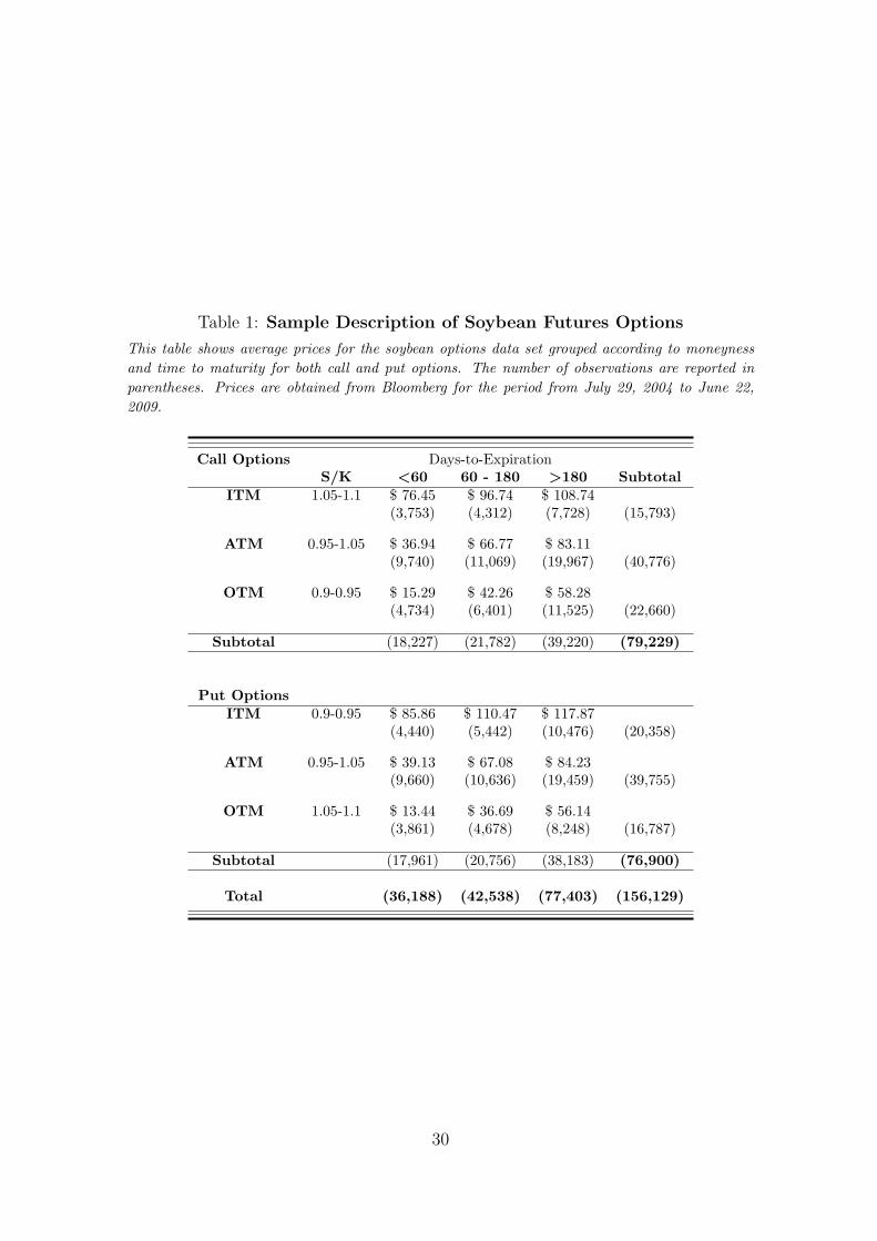
Table 1: Sample Description of Soybean Futures Options

This table shows average prices for the soybean options data set grouped according to moneynessand time to maturity for both call and put options. The number of observations are reported inparentheses. Prices are obtained from Bloomberg for the period from July 29, 2004 to June 22,2009.

Call Options Days-to-ExpirationS/K <60 60 - 180 >180 Subtotal

ITM 1.05-1.1 $ 76.45 $ 96.74 $ 108.74(3,753) (4,312) (7,728) (15,793)

ATM 0.95-1.05 $ 36.94 $ 66.77 $ 83.11(9,740) (11,069) (19,967) (40,776)

OTM 0.9-0.95 $ 15.29 $ 42.26 $ 58.28(4,734) (6,401) (11,525) (22,660)

Subtotal (18,227) (21,782) (39,220) (79,229)

Put OptionsITM 0.9-0.95 $ 85.86 $ 110.47 $ 117.87

(4,440) (5,442) (10,476) (20,358)

ATM 0.95-1.05 $ 39.13 $ 67.08 $ 84.23(9,660) (10,636) (19,459) (39,755)

OTM 1.05-1.1 $ 13.44 $ 36.69 $ 56.14(3,861) (4,678) (8,248) (16,787)

Subtotal (17,961) (20,756) (38,183) (76,900)

Total (36,188) (42,538) (77,403) (156,129)

30

Table 2: Sample Description of Heating Oil Futures Options

This table shows average prices for the heating oil options data set grouped according to moneynessand time to maturity for both call and put options. The number of observations are reported inparentheses. Prices are obtained from Bloomberg for the period from October 21, 2004 to December26, 2006.

Call Options Days-to-ExpirationS/K <60 60 - 180 >180 Subtotal

ITM 1.05-1.1 $ 15.05 $ 20.89 $ 25.51(5,517) (9,692) (5,153) (20,362)

ATM 0.95-1.05 $ 7.42 $ 13.55 $ 17.88(14,867) (29,388) (19,144) (63,399)

OTM 0.9-0.95 $ 3.24 $ 8.47 $ 13.04(7,877) (16,758) (9,321) (33,956)

Subtotal (28,261) (55,838) (33,618) (117,717)

Put OptionsITM 0.9-0.95 $ 16.06 $ 20.34 $ 23.66

(4,739) (5,893) (1,751) (12,383)

ATM 0.95-1.05 $ 7.26 $ 12.26 $ 16.42(13,009) (20,195) (12,130) (45,334)

OTM 1.05-1.1 $ 2.94 $ 7.57 $ 12.04(5,892) (12,005) (9,272) (27,169)

Subtotal (23,640) (38,093) (23,153) (84,886)

Total (51,901) (93,931) (56,771) (202,603)

31

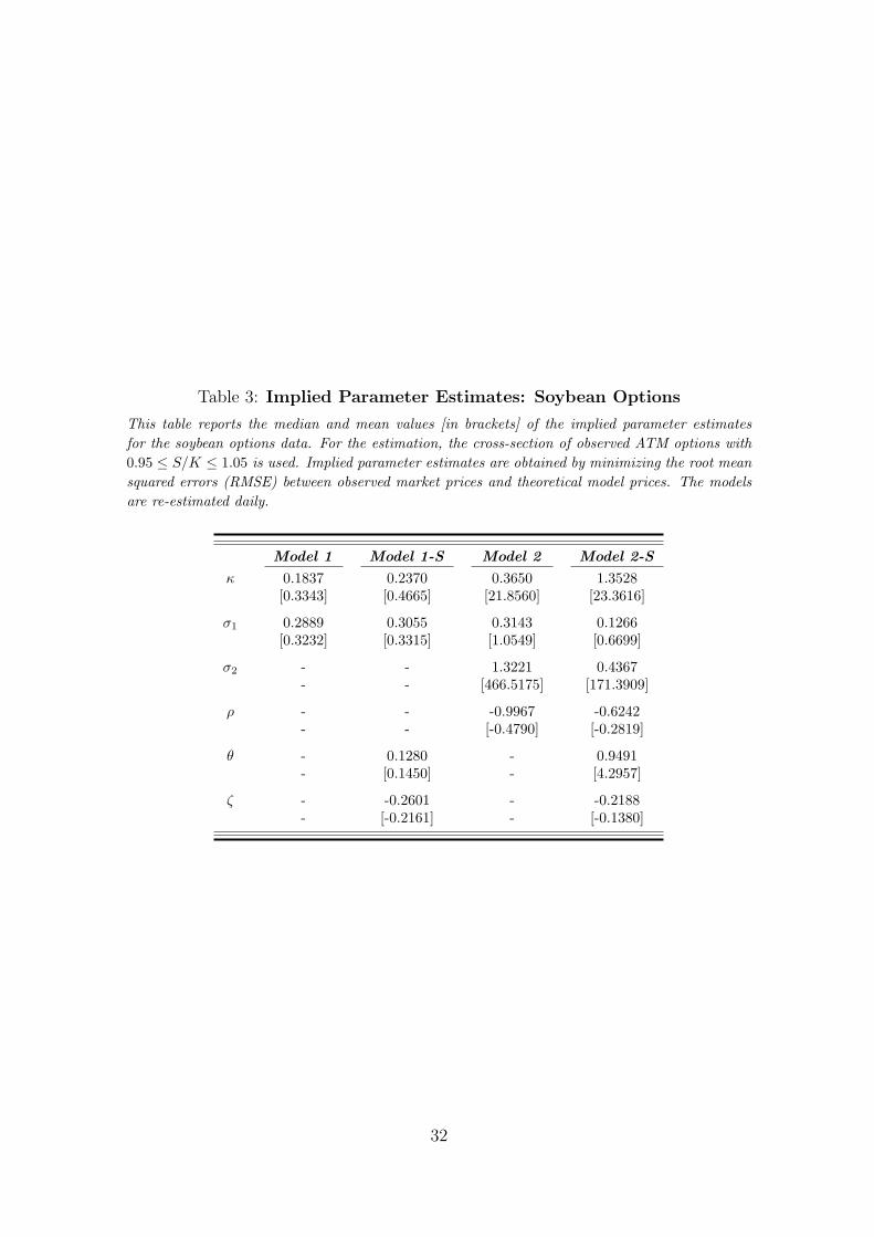
Table 3: Implied Parameter Estimates: Soybean Options

This table reports the median and mean values [in brackets] of the implied parameter estimatesfor the soybean options data. For the estimation, the cross-section of observed ATM options with0.95 ≤ S/K ≤ 1.05 is used. Implied parameter estimates are obtained by minimizing the root meansquared errors (RMSE) between observed market prices and theoretical model prices. The modelsare re-estimated daily.

Model 1 Model 1-S Model 2 Model 2-S

κ 0.1837 0.2370 0.3650 1.3528[0.3343] [0.4665] [21.8560] [23.3616]

σ1 0.2889 0.3055 0.3143 0.1266[0.3232] [0.3315] [1.0549] [0.6699]

σ2 - - 1.3221 0.4367- - [466.5175] [171.3909]

ρ - - -0.9967 -0.6242- - [-0.4790] [-0.2819]

θ - 0.1280 - 0.9491- [0.1450] - [4.2957]

ζ - -0.2601 - -0.2188- [-0.2161] - [-0.1380]

32

Table 4: Implied Parameter Estimates: Heating Oil Options

This table reports the median and mean values [in brackets] of the implied parameter estimates forthe heating oil options data. For the estimation, the cross-section of observed ATM options with0.95 ≤ S/K ≤ 1.05 is used. Implied parameter estimates are obtained by minimizing the root meansquared errors (RMSE) between observed market prices and theoretical model prices. The modelsare re-estimated daily.

Model 1 Model 1-S Model 2 Model 2-S

κ 0.4624 0.4929 1.3104 0.9520[0.5533] [0.5699] [2.1311] [3.8557]

σ1 0.3436 0.3619 0.3185 0.1252[0.3750] [0.3709] [0.3370] [0.2185]

σ2 - - 0.4366 0.3789- - [0.5322] [0.4553]

ρ - - -0.5729 -0.3629- - [-0.3536] [-0.0474]

θ - 0.1162 - 1.0182- [0.1459] - [2.1224]

ζ - 0.2681 - 0.2606- [0.2039] - [0.2059]

33

Tab

le5:

In-S

am

ple

Pri

cing

Err

ors

:Soybean

Opti

ons

Thi

sta

ble

disp

lays

the

in-s

ampl

epr

icin

ger

rors

ofop

tion

son

soyb

ean

futu

res.

Pri

cing

erro

rsar

ere

port

edas

root

mea

nsq

uare

der

rors

(RM

SE)

and

rela

tive

root

mea

nsq

uare

der

rors

(RR

MSE

)of

option

pric

esfo

rth

efo

urva

luat

ion

mod

els.

The

repo

rted

pric

ing

erro

rsar

eca

lcul

ated

asav

erag

eva

lues

over

the

peri

odfrom

July

29,20

04to

June

22,20

09.

Pri

cing

erro

rsar

egr

oupe

dby

mat

urity

and

mon

eyne

ssof

the

option

s.O

nly

AT

Mpr

ices

wer

eus

edfo

rth

epa

ram

eter

estim

atio

n.

Day

s-to

-Expir

atio

n<

6060

-18

0>

180

Subto

tal

RM

SE

RR

MSE

RM

SE

RR

MSE

RM

SE

RR

MSE

RM

SE

RR

MSE

[$]

[%]

[$]

[%]

[$]

[%]

[$]

[%]

OT

M

Model1

2.15

37.0

53.

3214

.25

5.47

14.6

54.

4922

.60

Model1-S

1.70

27.9

72.

9812

.63

4.85

12.4

03.

9517

.96

Model2

1.89

34.0

73.

2113

.71

5.20

14.6

14.

3121

.51

Model2-S

1.52

26.7

92.

8612

.51

4.42

12.3

13.

6417

.12

AT

M

Model1

2.62

16.1

82.

716.

104.

678.

244.

0511

.59

Model1-S

1.84

11.1

22.

134.

493.

826.

763.

278.

63M

odel2

2.28

13.6

92.

525.

574.

308.

143.

7910

.56

Model2-S

1.51

9.54

1.88

4.19

3.33

6.50

2.84

7.62

ITM

Model1

2.46

3.20

3.48

3.79

6.26

5.95

5.09

5.36

Model1-S

2.06

2.59

3.24

3.46

5.61

5.24

4.58

4.70

Model2

2.28

2.96

3.39

3.70

5.87

5.81

4.88

5.23

Model2-S

1.94

2.50

3.16

3.43

5.05

4.97

4.25

4.52

Subto

talM

odel1

2.55

22.1

33.

138.

755.

3810

.25

4.50

14.8

5M

odel1-S

1.93

16.3

92.

717.

474.

678.

673.

8711

.62

Model2

2.27

19.7

62.

998.

355.

0510

.20

4.29

13.9

4M

odel2-S

1.71

15.1

92.

567.

344.

198.

523.

5210

.89

34

Tab

le6:

In-S

am

ple

Pri

cing

Err

ors

:H

eati

ng

Oil

Opti

ons

Thi

sta

ble

disp

lays

the

in-s

ampl

epr

icin

ger

rors

ofop

tion

son

heat

ing

oilf

utur

es.

Pri

cing

erro

rsar

ere

port

edas

root

mea

nsq

uare

der

rors

(RM

SE)

and

rela

tive

root

mea

nsq

uare

der

rors

(RR

MSE

)of

option

pric

esfo

rth

efo

urva

luat

ion

mod

els.

The

repo

rted

pric

ing

erro

rsar

eca

lcul

ated

asav

erag

eva

lues

over

the

peri

odfrom

Oct

ober

21,20

04to

Dec

embe

r26

,20

06.

Pri

cing

erro

rsar

egr

oupe

dby

mat

urity

and

mon

eyne

ssof

the

option

s.O

nly

AT

Mpr

ices

wer

eus

edfo

rth

epa

ram

eter

estim

atio

n.

Day

s-to

-Expir

atio

n<

6060

-18

0>

180

Subto

tal

RM

SE

RR

MSE

RM

SE

RR

MSE

RM

SE

RR

MSE

RM

SE

RR

MSE

[$]

[%]

[$]

[%]

[$]

[%]

[$]

[%]

OT

M

Model1

0.37

15.9

70.

6117

.35

0.72

6.15

0.66

18.2

4M

odel1-S

0.24

10.6

80.

5316

.21

0.58

5.01

0.54

15.5

5M

odel2

0.24

9.54

0.57

16.5

00.

595.

150.

5715

.32

Model2-S

0.19

7.44

0.51

16.0

80.

534.

630.

5014

.27

AT

M

Model1

0.40

7.52

0.49

5.70

0.71

5.55

0.60

7.76

Model1-S

0.21

4.34

0.34

4.33

0.53

4.47

0.43

5.78

Model2

0.26

4.45

0.38

4.63

0.58

4.69

0.48

5.96

Model2-S

0.13

2.41

0.28

3.84

0.48

4.12

0.37

4.75

ITM

Model1

0.36

2.42

0.43

2.11

0.66

2.77

0.50

2.51

Model1-S

0.21

1.34

0.34

1.57

0.49

2.04

0.36

1.72

Model2

0.23

1.46

0.38

1.76

0.55

2.24

0.41

1.92

Model2-S

0.16

0.96

0.31

1.44

0.44

1.84

0.33

1.51

Subto

talM

odel1

0.39

10.0

30.

5411

.38

0.74

5.93

0.62

12.3

9M

odel1-S

0.23

6.48

0.43

10.2

70.

584.

910.

4810

.36

Model2

0.25

6.02

0.47

10.5

30.

615.

070.

5310

.32

Model2-S

0.16

4.32

0.39

10.0

30.

534.

560.

449.

39

35

Tab

le7:

Out-

of-Sam

ple

Pri

cing

Err

ors

:Soybean

Opti

ons

Thi

sta

ble

repo

rts

the

out-of

-sam

ple

pric

ing

erro

rsof

option

son

soyb

ean

futu

res.

Pri

cing

erro

rsar

ere

port

edas

root

mea

nsq

uare

der

rors

(RM

SE)

and

rela

tive

root

mea

nsq

uare

der

rors

(RR

MSE

)of

option

pric

esfo

rth

efo

urva

luat

ion

mod

els.

The

repo

rted

pric

ing

erro

rsar

eca

lcul

ated

asav

erag

eva

lues

duri

ngth

epe

riod

from

July

30,20

04to

June

22,20

09.

Pri

cing

erro

rsar

egr

oupe

dby

mat

urity

and

mon

eyne

ssof

the

option

s.T

heor

etic

alm

odel

base

dpr

ices

are

deri

ved

byus

ing

para

met

ers

estim

ated

the

day

befo

re.

Day

s-to

-Expir

atio

n<

6060

-18

0>

180

Subto

tal

RM

SE

RR

MSE

RM

SE

RR

MSE

RM

SE

RR

MSE

RM

SE

RR

MSE

[$]

[%]

[$]

[%]

[$]

[%]

[$]

[%]

OT

M

Model1

2.31

38.2

93.

5715

.04

5.81

15.2

44.

8023

.55

Model1-S

1.97

30.0

63.

2913

.54

5.29

13.1

74.

3419

.39

Model2

2.13

35.8

43.

5014

.62

5.60

15.3

44.

6622

.87

Model2-S

1.85

29.2

03.

2113

.53

4.99

13.3

04.

1218

.90

AT

M

Model1

2.83

16.8

83.

076.

695.

228.

814.

5012

.27

Model1-S

2.23

12.3

62.

645.

354.

677.

623.

949.

75M

odel2

2.60

14.9

92.

956.

325.

028.

864.

3611

.59

Model2-S

2.08

11.8

62.

535.

304.

367.

573.

689.

29

ITM

Model1

2.60

3.35

3.74

4.04

6.60

6.20

5.38

5.61

Model1-S

2.31

2.86

3.55

3.75

6.07

5.61

4.96

5.06

Model2

2.48

3.18

3.69

3.99

6.25

6.09

5.21

5.54

Model2-S

2.24

2.84

3.50

3.75

5.62

5.42

4.71

4.95

Subto

talM

odel1

2.73

22.9

23.

439.

335.

8110

.75

4.87

15.5

3M

odel1-S

2.25

17.7

83.

118.

195.

279.

374.

3712

.69

Model2

2.54

21.1

33.

359.

035.

5710

.80

4.72

14.9

5M

odel2-S

2.13

17.2

93.

038.

194.

949.

394.

1312

.34

36

Tab

le8:

Out-

of-Sam

ple

Pri

cing

Err

ors

:H

eati

ng

Oil

Opti

ons

Thi

sta

ble

repo

rts

the

out-of

-sam

ple

pric

ing

erro

rsof

option

son

heat

ing

oilfu

ture

s.Pri

cing

erro

rsar

ere

port

edas

root

mea

nsq

uare

der

rors

(RM

SE)

and

rela

tive

root

mea

nsq

uare

der

rors

(RR

MSE

)of

option

pric

esfo

rth

efo

urva

luat

ion

mod

els.

The

repo

rted

pric

ing

erro

rsar

eca

lcul

ated

asav

erag

eva

lues

duri

ngth

epe

riod

from

Oct

ober

22,20

04to

Dec

embe

r26

,20

06.

Pri

cing

erro

rsar

egr

oupe

dby

mat

urity

and

mon

eyne

ssof

the

option

s.T

heor

etic

alm

odel

base

dpr

ices

are

deri

ved

byus

ing

para

met

ers

estim

ated

the

day

befo

re.

Day

s-to

-Expir

atio

n<

6060

-18

0>

180

Subto

tal

RM

SE

RR

MSE

RM

SE

RR

MSE

RM

SE

RR

MSE

RM

SE

RR

MSE

[$]

[%]

[$]

[%]

[$]

[%]

[$]

[%]

OT

M

Model1

0.40

16.6

30.

6317

.71

0.74

6.32

0.68

18.6

6M

odel1-S

0.28

11.6

00.

5616

.69

0.60

5.22

0.57

16.1

1M

odel2

0.29

10.8

30.

6016

.88

0.62

5.38

0.61

15.9

9M

odel2-S

0.25

9.10

0.55

16.5

50.

564.

890.

5515

.08

AT

M

Model1

0.43

7.89

0.53

6.04

0.75

5.81

0.65

8.13

Model1-S

0.27

5.04

0.41

4.91

0.60

4.89

0.51

6.38

Model2

0.31

5.23

0.44

5.12

0.64

5.07

0.55

6.56

Model2-S

0.22

3.68

0.37

4.55

0.56

4.61

0.47

5.64

ITM

Model1

0.39

2.55

0.46

2.27

0.68

2.88

0.53

2.66

Model1-S

0.25

1.58

0.39

1.83

0.52

2.18

0.41

1.96

Model2

0.27

1.71

0.42

1.95

0.57

2.38

0.45

2.13

Model2-S

0.21

1.32

0.37

1.73

0.48

2.02

0.38

1.81

Subto

talM

odel1

0.42

10.4

80.

5811

.70

0.77

6.14

0.66

12.7

4M

odel1-S

0.28

7.17

0.48

10.7

40.

635.

220.

5410

.87

Model2

0.30

6.90

0.51

10.9

10.

665.

370.

5810

.88

Model2-S

0.23

5.55

0.46

10.5

30.

584.

920.

5110

.10

37

Tab

le9:

Reduct

ion

ofP

rici

ng

Err

ors

:Soybean

Opti

ons

Thi

sta

ble

show

sth

epe

rcen

tage

redu

ctio

nin

root

mea

nsq

uare

der

rors

(RM

SE)

for

option

son

soyb

ean

futu

res

due

toth

em

odel

exte

nsio

ns.

The

resp

ective

RM

SEar

ere

port

edin

Tab

les

5an

d7.

The

figur

esar

egr

oupe

dby

mat

urity

and

mon

eyne

ssof

the

option

san

dar

ere

port

edfo

rth

ein

-sam

ple

and

out-of

-sam

ple

pric

ing

erro

rs.

*in

dica

tes

sign

ifica

nce

atth

e1%

leve

lac

cord

ing

toa

Wilc

oxon

sign

ed-r

ank

test

.

In-S

ample

Out-

of-S

ample

Day

s-to

-Expir

atio

nD

ays-

to-E

xpir

atio

n<

6060

-18

0>

180

Subto

tal

<60

60-

180

>18

0Subto

tal

Intr

oduct

ion

ofSea

sonal

Vol

atility

One-

Fac

tor

AT

M30

.01%

∗21

.21%

∗18

.09%

∗19

.20%

∗21

.28%

∗13

.95%

∗10

.61%

∗12

.43%

∗

All

24.3

2%∗

13.1

5%∗

13.1

5%∗

14.0

8%∗

17.3

6%∗

9.47

%∗

9.20

%∗

10.2

6%∗

Tw

o-Fac

tor

AT

M33

.64%

∗25

.38%

∗22

.57%

∗25

.09%

∗20

.13%

∗14

.24%

∗13

.13%

∗15

.60%

∗

All

24.6

8%∗

14.5

2%∗

16.9

6%∗

17.9

6%∗

15.8

4%∗

9.50

%∗

11.3

3%∗

12.4

7%∗

Intr

oduct

ion

of2n

dFac

tor

w/o

Sea

sonal

Vol

atility

AT

M13

.05%

∗6.

80%∗

7.83

%∗

6.38

%∗

8.07

%∗

3.75

%∗

3.93

%∗

3.04

%∗

All

11.0

8%∗

4.24

%∗

6.15

%∗

4.81

%∗

7.03

%∗

2.50

%∗

4.10

%∗

2.98

%∗

wit

hSea

sonal

Vol

atility

AT

M17

.56%

∗11

.74%

∗12

.88%

∗13

.20%

∗6.

73%∗

4.08

%∗

6.64

%∗

6.55

%∗

All

11.5

1%∗

5.75

%∗

10.2

7%∗

9.11

%∗

5.32

%∗

2.53

%∗

6.35

%∗

5.36

%∗

38

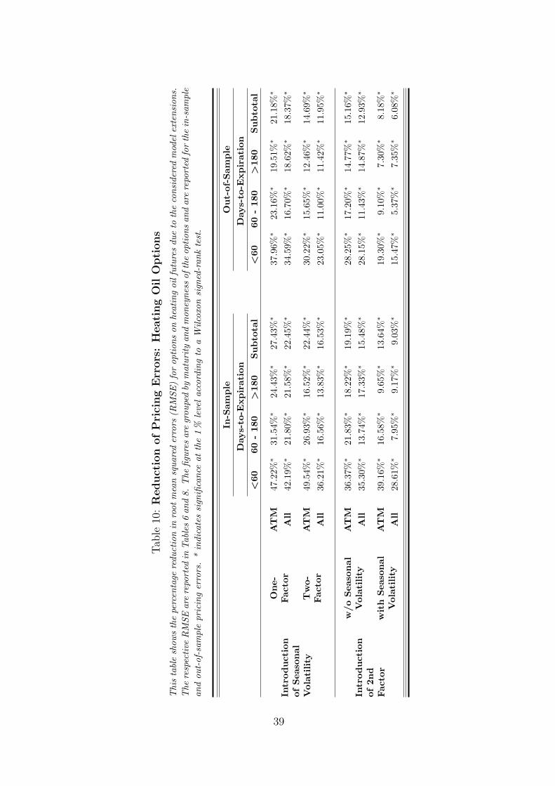
Tab

le10

:R

educt

ion

ofP

rici

ng

Err

ors

:H

eati

ng

Oil

Opti

ons

Thi

sta

ble

show

sth

epe

rcen

tage

redu

ctio

nin

root

mea

nsq

uare

der

rors

(RM

SE)fo

rop

tion

son

heat

ing

oilf

utur

esdu

eto

the

cons

ider

edm

odel

exte

nsio

ns.

The

resp

ective

RM

SEar

ere

port

edin

Tab

les6

and

8.T

hefig

ures

are

grou

ped

bym

atur

ity

and

mon

eyne

ssof

the

option

san

dar

ere

port

edfo

rth

ein

-sam

ple

and

out-of

-sam

ple

pric

ing

erro

rs.

*in

dica

tes

sign

ifica

nce

atth

e1%

leve

lac

cord

ing

toa

Wilc

oxon

sign

ed-r

ank

test

.

In-S

ample

Out-

of-S

ample

Day

s-to

-Expir

atio

nD

ays-

to-E

xpir

atio

n<

6060

-18

0>

180

Subto

tal

<60

60-

180

>18

0Subto

tal

Intr

oduct

ion

ofSea

sonal

Vol

atility

One-

Fac

tor

AT

M47

.22%

∗31

.54%

∗24

.43%

∗27

.43%

∗37

.96%

∗23

.16%

∗19

.51%

∗21

.18%

∗

All

42.1

9%∗

21.8

0%∗

21.5

8%∗

22.4

5%∗

34.5

9%∗

16.7

0%∗

18.6

2%∗

18.3

7%∗

Tw

o-Fac

tor

AT

M49

.54%

∗26

.93%

∗16

.52%

∗22

.44%

∗30

.22%

∗15

.65%

∗12

.46%

∗14

.69%

∗

All

36.2

1%∗

16.5

6%∗

13.8

3%∗

16.5

3%∗

23.0

5%∗

11.0

0%∗

11.4

2%∗

11.9

5%∗

Intr

oduct

ion

of2n

dFac

tor

w/o

Sea

sonal

Vol

atility

AT

M36

.37%

∗21

.83%

∗18

.22%

∗19

.19%

∗28

.25%

∗17

.20%

∗14

.77%

∗15

.16%

∗

All

35.3

0%∗

13.7

4%∗

17.3

3%∗

15.4

8%∗

28.1

5%∗

11.4

3%∗

14.8

7%∗

12.9

3%∗

wit

hSea

sonal

Vol

atility

AT

M39

.16%

∗16

.58%

∗9.

65%∗

13.6

4%∗

19.3

0%∗

9.10

%∗

7.30

%∗

8.18

%∗

All

28.6

1%∗

7.95

%∗

9.17

%∗

9.03

%∗

15.4

7%∗

5.37

%∗

7.35

%∗

6.08

%∗

39