Seasonal and diurnal water quality and ecological dynamics along … · 2017-01-20 · valuable...

Procedia Environmental Sciences 13 (2012) 899 – 918

1878-0296 © 2011 Published by Elsevier B.V. Selection and/or peer-review under responsibility of School of Environment, Beijing Normal University.doi:10.1016/j.proenv.2012.01.084

Available online at www.sciencedirect.com

Procedia Environmental

Sciences Procedia Environmental Sciences 8 (2011) 926–945

www.elsevier.com/locate/procedia

The 18th Biennial Conference of International Society for Ecological Modelling

Seasonal and diurnal water quality and ecological dynamics along a salinity gradient (Mira channel, Aveiro lagoon,

Portugal) M. Rodriguesa*, A. Oliveiraa, H. Queirogab, V. Brotasc,d

aHydraulics and Environment Department – National Laboratory for Civil Enginnering, Avenida do Brasil 101, 1700-066 Lisbon, Portugal

bCESAM&Biology Department – University of Aveiro, Campus Universitário de Santiago, 3810-193 Aveiro, Portugal cUniversity of Lisbon, Faculdade de Ciências, Center of Oceanography, Campo Grande, 1749-016 Lisboa, Portugal

dPlymouth Marine Laboratory, Prospect Place, Plymouth, United Kingdom

Abstract

The patterns of water quality and ecological dynamics in estuaries vary at different time scales. Characterizing this variability at short (diurnal and seasonal) time scales is a pre-requisite to investigate the effects of long-term climate changes. Seasonal scales depend mostly on the natural climatic variability, while diurnal scales are generally associated with the tidal cycle and wind events. In order to study the role of these superimposed scales in the Aveiro lagoon, an integrated approach, which combines data acquisition and numerical modelling, was followed. The analysis was conducted with the three-dimensional, fully coupled hydrodynamic and ecological numerical model, ECO-SELFE, extended to account for the oxygen cycle. For data acquisition three field campaigns were performed along a salinity gradient (Mira channel), covering different seasonal situations: March 2009, September 2009 and January 2010. These campaigns, each lasting 24 hours, included the measurement of physical, chemical and biological parameters (river flow, water levels, currents velocities, water temperature, salinity, dissolved oxygen, nutrients and chlorophyll a). Results show the ability of the model to represent both the spatial and temporal patterns observed for the different variables. Chlorophyll a and nutrients tend to present larger concentrations upstream than downstream, with the largest values observed in spring. The distribution patterns are significantly influenced by the tidal dynamics. © 2011 Published by Elsevier Ltd. Keywords: Chlorophyll a; Dissolved Oxygen; Nutrients; Tide

* Corresponding author. Tel.: +351218443613; fax: +351218443016. E-mail address: [email protected].

© 2011 Published by Elsevier B.V. Selection and/or peer-review under responsibility of School of Environment, Beijing Normal University. Open access under CC BY-NC-ND license.

Open access under CC BY-NC-ND license.

http://creativecommons.org/licenses/by-nc-nd/3.0/

http://creativecommons.org/licenses/by-nc-nd/3.0/

900 M. Rodrigues et al. / Procedia Environmental Sciences 13 (2012) 899 – 918 M. Rodrigues et al./ Procedia Environmental Sciences 8 (2011) 926–945 927

1. Introduction

The complex dynamics of estuarine ecosystems depends on the interaction between several factors, being influenced by both natural forcings and anthropogenic activities. Among the natural forcings the combined effect of ocean tides and river flows is one of the main drivers of the estuarine dynamics. Estuaries also present attractive resources for human activities and are subject to different pressures, which may contribute to significant changes on their ecological quality and dynamics (e.g wastewater discharges, river flow regulation, sand extraction and other dredging activities).

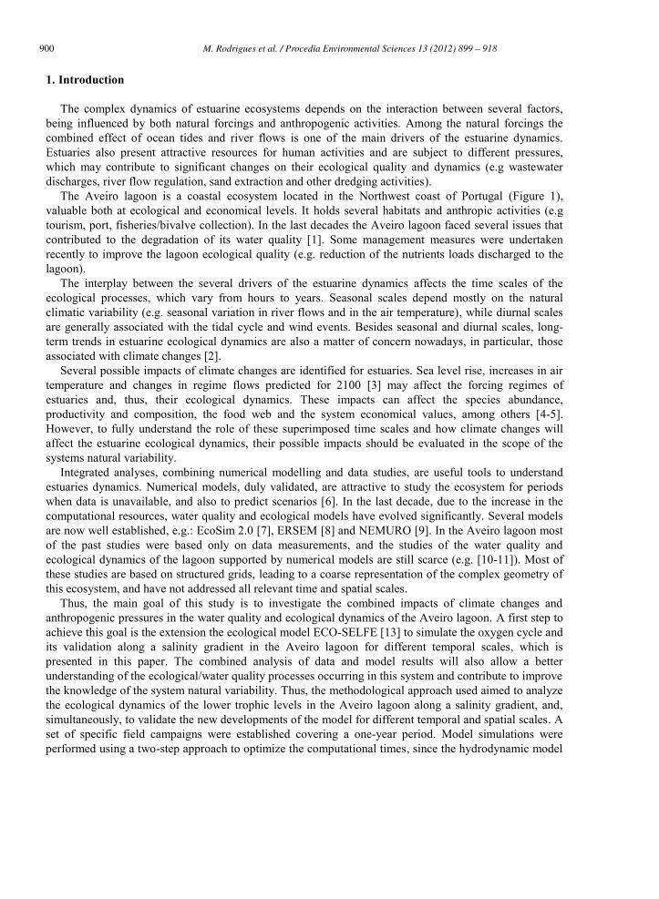
The Aveiro lagoon is a coastal ecosystem located in the Northwest coast of Portugal (Figure 1), valuable both at ecological and economical levels. It holds several habitats and anthropic activities (e.g tourism, port, fisheries/bivalve collection). In the last decades the Aveiro lagoon faced several issues that contributed to the degradation of its water quality [1]. Some management measures were undertaken recently to improve the lagoon ecological quality (e.g. reduction of the nutrients loads discharged to the lagoon).

The interplay between the several drivers of the estuarine dynamics affects the time scales of the ecological processes, which vary from hours to years. Seasonal scales depend mostly on the natural climatic variability (e.g. seasonal variation in river flows and in the air temperature), while diurnal scales are generally associated with the tidal cycle and wind events. Besides seasonal and diurnal scales, long-term trends in estuarine ecological dynamics are also a matter of concern nowadays, in particular, those associated with climate changes [2].

Several possible impacts of climate changes are identified for estuaries. Sea level rise, increases in air temperature and changes in regime flows predicted for 2100 [3] may affect the forcing regimes of estuaries and, thus, their ecological dynamics. These impacts can affect the species abundance, productivity and composition, the food web and the system economical values, among others [4-5]. However, to fully understand the role of these superimposed time scales and how climate changes will affect the estuarine ecological dynamics, their possible impacts should be evaluated in the scope of the systems natural variability.

Integrated analyses, combining numerical modelling and data studies, are useful tools to understand estuaries dynamics. Numerical models, duly validated, are attractive to study the ecosystem for periods when data is unavailable, and also to predict scenarios [6]. In the last decade, due to the increase in the computational resources, water quality and ecological models have evolved significantly. Several models are now well established, e.g.: EcoSim 2.0 [7], ERSEM [8] and NEMURO [9]. In the Aveiro lagoon most of the past studies were based only on data measurements, and the studies of the water quality and ecological dynamics of the lagoon supported by numerical models are still scarce (e.g. [10-11]). Most of these studies are based on structured grids, leading to a coarse representation of the complex geometry of this ecosystem, and have not addressed all relevant time and spatial scales.

Thus, the main goal of this study is to investigate the combined impacts of climate changes and anthropogenic pressures in the water quality and ecological dynamics of the Aveiro lagoon. A first step to achieve this goal is the extension the ecological model ECO-SELFE [13] to simulate the oxygen cycle and its validation along a salinity gradient in the Aveiro lagoon for different temporal scales, which is presented in this paper. The combined analysis of data and model results will also allow a better understanding of the ecological/water quality processes occurring in this system and contribute to improve the knowledge of the system natural variability. Thus, the methodological approach used aimed to analyze the ecological dynamics of the lower trophic levels in the Aveiro lagoon along a salinity gradient, and, simultaneously, to validate the new developments of the model for different temporal and spatial scales. A set of specific field campaigns were established covering a one-year period. Model simulations were performed using a two-step approach to optimize the computational times, since the hydrodynamic model

901M. Rodrigues et al. / Procedia Environmental Sciences 13 (2012) 899 – 918928 M. Rodrigues et al./ Procedia Environmental Sciences 8 (2011) 926–945

is about 2-3 times faster than the coupled hydrodynamic-ecological model. Thus, validation was performed first for the hydrodynamic model and then for the coupled model.

a) -9.5 -9 -8.5 -8 -7.539

39.5

40

40.5

41

41.5

42

Por

tuga

l

Aveiro Lagoon

b)

Mira Channel

Ílhavo Channel

S. Jacinto Channel

Espinheiro Channel

Boco River

Vouga River

Antuã River

CasterRiver

Mira

2

1

43

1. EM12. EM23. EB 4. EM3

Figure 1. Location of the: (a) Aveiro lagoon and (b) sampling stations along the Mira channel.

2. Study area

The Aveiro lagoon is about 45 km long and 10 km wide, covering an area that, during spring tides, varies from 66 km2 at low tide to 83 km2 at high tide [12]. The lagoon is separated from the sea by a sandbar and connects to it through an artificial inlet. From this inlet the lagoon spreads in four main branches: Mira, S. Jacinto, Ílhavo and Espinheiro channels (Figure 1b). These four main channels have several narrow channels and interconnections enhancing the complexity of this system. The exception is the Mira channel which behaves as a sub-estuarine system, and for this reason was chosen to the development of this study. The lagoon is very shallow with mean depths of 1 m [13] and maximum depths of about 20 m in the artificial channel near the inlet. Tides at the mouth are semi-diurnal ranging from 0.6 m in neap tides to 3.2 m in spring tides, and have a mean tidal range of 2 m [15]. The tidal prism in the mouth is of about 70x106 m3 in spring tides, 10% of which flows to the Mira channel [15]. Freshwater flows into the lagoon from the upstream areas of the four main channels. The main sources of freshwater are the rivers Vouga and Antuã [14-15], but some uncertainty remains about the flows in the lagoon. Annual average flows found in the literature vary from 29-50 m3 s-1 for the Vouga river, and from 2-5 m3 s-1 for the Antuã river [14-15]. In the other channels the river flows are lower, but there is a significant lack of data. In the Mira channel, in particular, the freshwater flow is poorly known [14]. Residence times in the lagoon, defined as [14], vary from less than 2 days near the mouth to more than 1 week in the upstream areas of the channels. More detailed descriptions of the lagoon can be found in [15] and references therein.

3. Description of the field campaigns

Three field campaigns were performed in the Mira channel on: March 29-31, 2009, September 15-17, 2009, and January 27-29, 2010. Samplings of physical, chemical and biological parameters were collected at four stations (Figure 1b). Additionally, the main rivers flowing into the lagoon were also sampled: Poço


da Cruz (Mira), Ouca (Boco), Angeja (Vouga), Estarreja (Antuã) and Ribeira-Ovar (Caster), to provide boundary conditions for the model.

At the stations along the Mira channel, measurements were performed during a 24 hour period and started on the second day of the campaign. The exception was station EM3 (Navio-Museu) where measurements of water levels started in the first day of the campaigns and lasted for 42 hours periods with 10 minute intervals (pressure gauge – LevelTroll 500). Water levels and current velocities (electromagnetic current meter) were measured with 1 hour intervals at station EB (Costa Nova). At stations EM2 (Vagueira) and EM3 (Areão) water levels were measured with 3 hours intervals using graduate rulers. In-situ measurements of salinity, water temperature and dissolved oxygen were done at all stations using multiparametric probes (YSI 556 and STD Anderaa). At station EB, a CTD with a fluorimeter was also used (NXIC CTD). Water samples were collected at all stations. For chlorophyll a analysis, filtration of 0.5 l triplicate samples through Whatman GF/C filters was done. Sampling was performed at 2 levels in the water column (surface and bottom), with 3 hours intervals at EM stations. At station EB the sampling interval was lower (1 hour for in-situ measurements and 2 hours for water sampling) and was done at 3 levels (surface, mid-depth and bottom). At the rivers, flows were measured, water samples were collected and in-situ measurements of salinity, water temperature and dissolved oxygen were performed.

Water samples for the determination of chlorophyll a and nutrients concentrations were analysed in laboratory. Chlorophyll a was determined espectrophotometrically after extraction with 90% acetone (following [15]. Ammonium (NH4

+) was quantified following the indophenol blue method [16]. Nitrates (NO3

-), phosphates (PO43-) and silicates (SiO2) analyses were performed in an autoanalyser (FIAstar 5000

Analyzer). Nitrates (including nitrites) were determined by the sulfanilic acid method after reduction of nitrates to nitrites in a cadmium column [17]. Phosphates were determined by the molibdate blue method of [18]. Silicates were determined by reaction with molibdate, and then reduced to form a heteropoly blue complex [19].

4. Model description and implementation in the Aveiro lagoon

4.1. Physical and numerical formulation

ECO-SELFE couples the hydrodynamic model SELFE [20] (parallel version 3.1c, available at www.stccmop.org/CORIE/modeling/selfe/) and an ecological model. SELFE is an unstructured grid model that simulates the baroclinic circulation across river-to-ocean scales. The model solves the shallow water equations and computes the free surface elevation and the three-dimensional fields of velocity, salinity and temperature. The model has a user-defined transport module that allows the simulation of any given tracer:

CFzC

zzCw

yCv

xCu

tC

c

(1)

where C is a given tracer concentration, (u,v,w) is the velocity (m s-1), is the vertical eddy diffusivity (m2 s-1), Fc represents the horizontal diffusion term and ΛC is the sources and sinks term. The two models are coupled through the last term of Equation 1.

The ecological model formulation is derived from EcoSim 2.0 – Ecological Simulation [7]. In its base formulation EcoSim2.0 allows the simulation of several ecological tracers (phytoplankton,


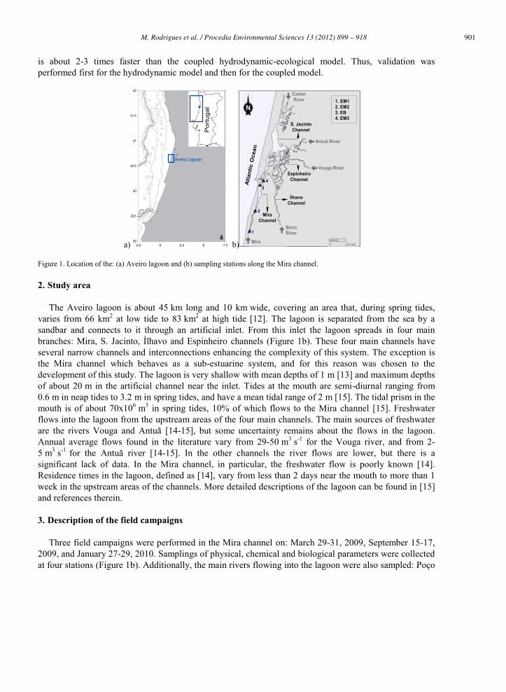
bacterioplankton, dissolved and particulate organic matter, inorganic nutrients and dissolved inorganic carbon) for the carbon, nitrogen, phosphorous, silica and iron cycles. In previous works this model was extended to simulate zooplankton tracers [21]. In the present study the model was extended to simulate the oxygen cycle due to its relevance in evaluating the ecological status of water bodies (e.g. Water Framework Directive). Thus, besides the ecological tracers of the EcoSim 2.0, ECO-SELFE also simulates several groups of zooplankton, dissolved oxygen and chemical oxygen demand. Figure 2 presents the source and sink terms of the ecological model and section 4.2 describes the recently implemented oxygen cycle.

Numerically ECO-SELFE uses a finite elements/finite volumes scheme. The domain is discretized horizontally with unstructured grids and vertically with hybrid SZ coordinates. Salinity and temperature advection can be solved with Eulerian-Lagragian Methods (ELM), upwind or TVD schemes. For ecological tracers only upwind and TVD schemes are available.

More detailed descriptions of the model formulation can be found in [7][13][22][23].

22

DOC1DOC2

22

DON1DON2DOP1

DissolvedOrganic Matter

PCiPNiPPiPSiiPFeiPiPgj

Phytoplankton

BCBNBPBFe

Bacterioplankton

DIC

DissolvedInorganic Carbon

FCkFNkFPkFSikFFek

Fecal OrganicMatter

NO3NH4DIPDISiDIFe

InorganicNutrient

CDOC1CDOC2

Colored DissolvedOrganic Carbon

Phot

osyn

thes

is

Photolysis

Uptake/Nitrification

State variables i – Phytoplankton groupsj – Individual pigment type

k – Class of fecal material

Mortality

ZClZNlZPl

Zooplankton

Grazing

l – Zooplankton groups

ATMOSPHERE

DO

DissolvedOxygen

CDO

Chemical OxygenDemand

SEDIMENTS

WATERCOLUMN

Rea

erat

ion

Rea

erat

ion

Sink

ing

Sink

ing

Sinking

Photolysis Regeneration

RespirationRespiration

Respiration

Reo

xida

tion

Growth/Lysis/Respiration

MortalityUptake

Denitrification

Nitr

ifica

tion

Predation/Respiration

Mor

talit

y

Lysi

s

Mortality

Mor

talit

y/Ex

cret

ion

Uptake

Excretion

Respiration/Grazing/Nitrification

Mortality/Excretion

Excretion

Mor

talit

y

Lysi

s

Figure 2. Source and sink terms of the ecological (black lines represent the previous variables of the model and blue lines represent the new variables for the oxygen cycle). C – Carbon, N – Nitrogen, P – Phosphorous, Si – Silica, Fe – Iron.

4.2. Oxygen cycle

4.2.1. Dissolved oxygen Dissolved oxygen (DO) is mainly defined as proposed by [22], considering an additional term relative

to re-aeration (physical exchanges with the atmosphere). The changes in the DO concentration result from


the gains due to the gross primary production and re-aeration (imposed only at the surface boundary), and the losses from phytoplankton, zooplankton and bacterioplankton respiration, the nitrification and the pelagic chemical reactions:

CODAtoNrespBfrespZrespPPCDO SO

ONB

OC

ll

OC

iiiir

OC

1

_ (2)

where ΛDO are the sources and sinks terms of DO (mmol O2 m-3), ΩO

C is the stoichiometric coefficient to convert carbon to oxygen units (mmol O2 mmol C-1), i is the phytoplankton groups index, μr_i is the realized growth rate of the phytoplankton group i (day-1), PCi is the phytoplankton carbon concentration of the group i (mmol C m-3), respPi is the respiration of the phytoplankton group i, fB is the oxygen regulating factor (non-dimensional, nd.), respB is the bacterioplankton respiration, l is the zooplankton groups index, respZl is the respiration of the zooplankton group l, reaer is the re-aeration, ΩO

N is the stoichiometric coefficient to convert nitrogen units to oxygen units (mmol O2 mmol N-1), AtoN is the nitrification (mmol N m-3), ΩS

O is the stoichiometric coefficient to convert sulfur to oxygen units (mmol S mmol O2

-1) and CDO is the chemical oxygen demand concentration (mmol O2 m-3). Phytoplankton respiration (respP) is defined as [24]:

)( _1010

iiiirPii

T

PiPii PCePCPCQbrespP

(3)

where bPi is the basal specific respiration rate (day-1), QPi is a temperature coefficient for phytoplankton (nd.), T is the water temperature (ºC), γPi is the fraction of assimilated production (nd.) and ei the excretion rate (day-1). The realized growth rate is defined as the minimum growth based on light or nutrient availability [7].

Zooplankton respiration (respZ) is defined as [24]:

llzZlZll

T

ZlZll ZCZCQbrespZ _1010

)1)(1(

(4)

where bZl is the basal specific respiration rate (day-1), Qzl is a temperature coefficient for zooplankton (nd.), ZCl is the zooplankton carbon concentration (mmol C.m-3), βZl is the excreted fraction of uptake (nd.), ηZl is the assimilation efficiency (nd.) and μz_l is the zooplankton growth rate due to food ingestion (day-1). The zooplankton growth rate due to food ingestion is calculated following [23]. The excreted fraction is defined as the ratio between the zooplankton growth and excretion rates (day-1).

Bacterioplankton respiration (respB) is defined as [24]:

BBOCCBB fGGEGGEBCQbrespB ))1(1( (5)

where bB is the basal specific respiration rate of bacterioplankton (day-1), QB is a temperature coefficient for bacterioplankton (nd.), GGEC is the growth efficiency (nd.), GGEC

O is the decrease in growth efficiency under anoxic conditions (nd.) and ρB is the bacterioplankton uptake. The bacterioplankton uptake is the defined as the minimum uptake from the available resources [7]. The oxygen regulating factor is calculated as [24]:


OsBB KDO

DOf_

3

3

(6)

where KsB_O is the half-saturation constant for oxygen limitation (mmol O2 m-3).

The oxygen reaeration (reaer) is imposed only at the surface boundary and is calculated as proposed by [23]:

)( DODODOKreaer wsatreaer (7)

where Kreaer is the reaeration coefficient (m.d-1), DOsat is the oxygen concentration at saturation (mmol O2 m-3), DOw is the increment to the saturation value due to the wind stress (mmol O2.m-3) and DO is the actual oxygen concentration. The use of DOw is optional and user-defined. Two alternative formulations are available for Kreaer [24][25]. DOsat is given by [26] and DOw is given by [25].

4.2.2. Chemical oxygen demand The chemical oxygen demand (COD) represents the reduced elements that can be oxidized by

inorganic means, implying the oxygen consumption. A similar approach to the one adopted by [24], where this variable is mostly regarded as sulfur (S), was chosen. The reduced elements are produced as a result of bacterial anoxic respiration and are used for the denitrification processes:

reoxAtoDenitrespBfCOD OC

SCB

OC

SC )1( (8)

where AtoDenit is the denitrification, reox is the reoxidation, ΩS

C is the stoichiometric coefficient to convert sulfur to carbon units (mmol S mmol C-1) and the first term represents the metabolic formation of reduction equivalents [24].

Denitrification and reoxidation are calculated as proposed by [24]:

3)1(1 NOrespBfDenitAtoDenit BOC

(9)

CODKDO

DOQCODreoxreoxCODS

T

COD_

1010

_

(10)

where Denit is the specific denitrification rate (day-1), Μ is the reference anoxic mineralization rate (mmol O2.m-3 day-1), reox_CDO is the specific reoxidation rate (d-1), QCDO is the a temperature constant for CDO (nd.) and Ks_CDO is the half-saturation constant for COD (mmol O2 m-3).

Changes in the ecological model implied also changes on other tracers formulations, namely phytoplankton, zooplankton, bacterioplankton, nitrates and dissolved inorganic carbon.

4.3. Model setup

The model setup was derived from [13]. The grid was refined and the bathymetry near the mouth was updated, based on 2008 data. For hydrodynamic simulations the horizontal domain was discretized in a


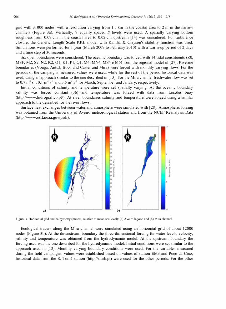
grid with 31000 nodes, with a resolution varying from 1.5 km in the coastal area to 2 m in the narrow channels (Figure 3a). Vertically, 7 equally spaced S levels were used. A spatially varying bottom roughness from 0.07 cm in the coastal area to 0.02 cm upstream [14] was considered. For turbulence closure, the Generic Length Scale KKL model with Kantha & Clayson's stability function was used. Simulations were performed for 1 year (March 2009 to February 2010) with a warm-up period of 2 days and a time step of 30 seconds.

Six open boundaries were considered. The oceanic boundary was forced with 14 tidal constituents (Z0, MSF, M2, S2, N2, K2, O1, K1, P1, Q1, M4, MN4, MS4 e M6) from the regional model of [27]. Riverine boundaries (Vouga, Antuã, Boco and Caster and Mira) were forced with monthly varying flows. For the periods of the campaigns measured values were used, while for the rest of the period historical data was used, using an approach similar to the one described in [13]. For the Mira channel freshwater flow was set to 0.7 m3 s-1, 0.1 m3 s-1 and 3.5 m3 s-1 for March, September and January, respectively.

Initial conditions of salinity and temperature were set spatially varying. At the oceanic boundary salinity was forced constant (36) and temperature was forced with data from Leixões buoy (http://www.hidrografico.pt/). At river boundaries salinity and temperature were forced using a similar approach to the described for the river flows.

Surface heat exchanges between water and atmosphere were simulated with [28]. Atmospheric forcing was obtained from the University of Aveiro meteorological station and from the NCEP Reanalysis Data (http://www.esrl.noaa.gov/psd/).

a) b)

Figure 3. Horizontal grid and bathymetry (meters, relative to mean sea level): (a) Aveiro lagoon and (b) Mira channel.

Ecological tracers along the Mira channel were simulated using an horizontal grid of about 12000 nodes (Figure 3b). At the downstream boundary the three-dimensional forcing for water levels, velocity, salinity and temperature was obtained from the hydrodynamic model. At the upstream boundary the forcing used was the one described for the hydrodynamic model. Initial conditions were set similar to the approach used in [13]. Monthly varying boundary conditions were used. For the variables measured during the field campaigns, values were established based on values of station EM3 and Poço da Cruz; historical data from the S. Tomé station (http://snirh.pt) were used for the other periods. For the other


variables a similar criteria to the one described by [13] was used. Input parameters of the ecological model were set as proposed by [13]. Since the model was updated to simulate the oxygen cycle, the input parameters the ecological processes added to the model are presented (Table 1). A sensitivity of the model results to basal phytoplankton respiration (bPi) and increase in the oxygen saturation concentration due to wind (DOw) was performed. A sensitivity analyses to other parameters had been performed previously [29].

Table 1. Input parameters – oxygen cycle [24][30].

bPi (day-1) QPi (-) γPi (-) bZl (day-1) QZl (-) ηZl (-) bB (day-1) QB (-) GGECO (-) KsB_O

(mmol O2 m-3)

0.01; 0.044 2.0 0.1 0.02 3.0 0.6 0.01 2.95 0.2 30.0

i = 1 (diatoms); l = 1 (copepods) bPi – phytoplankton basal specific respiration rate; QPi - temperature coefficient for phytoplankton; γPi – fraction of assimilated production; bZl – zooplankton basal specific respiration rate; Qzl – temperature coefficient for zooplankton; ηZl – assimilation efficiency; bB – bacterioplankton basal specific respiration rate; QB – temperature coefficient for bacterioplankton; GGEC

O – decrease in growth efficiency under anoxic conditions; KsB_O – half-saturation constant for oxygen limitation

5. Results and discussion

5.1. Hydrodynamics

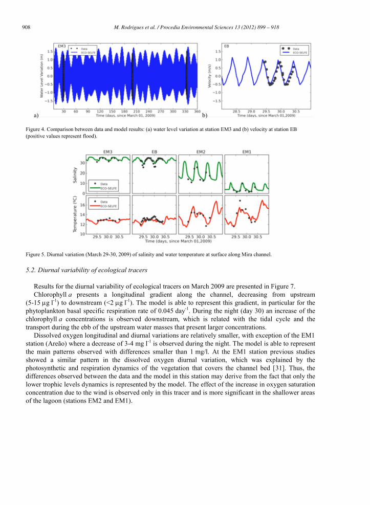
Water levels at station EM3 show the ability of the model to represent adequately tide both in terms of phase and amplitude (Figure 4a). Differences between data and model are generally smaller than 5-10 cm with mean absolute errors (MAE) of about 10 cm. From the downstream station to the upstream station tide has a delay of about 1-2 hours (results not shown). For currents velocity a good agreement between data and the model is also observed, with MAE of about 0.2 m s-1 (Figure 4b). Current velocity at station EB vary from 0.5 m/s during the ebb to 1 m s-1 during the flood. The differences observed may be due to changes in bathymetry along the channel, since the bathymetry available for this channel (from 1987/88) is not contemporary of the campaigns.

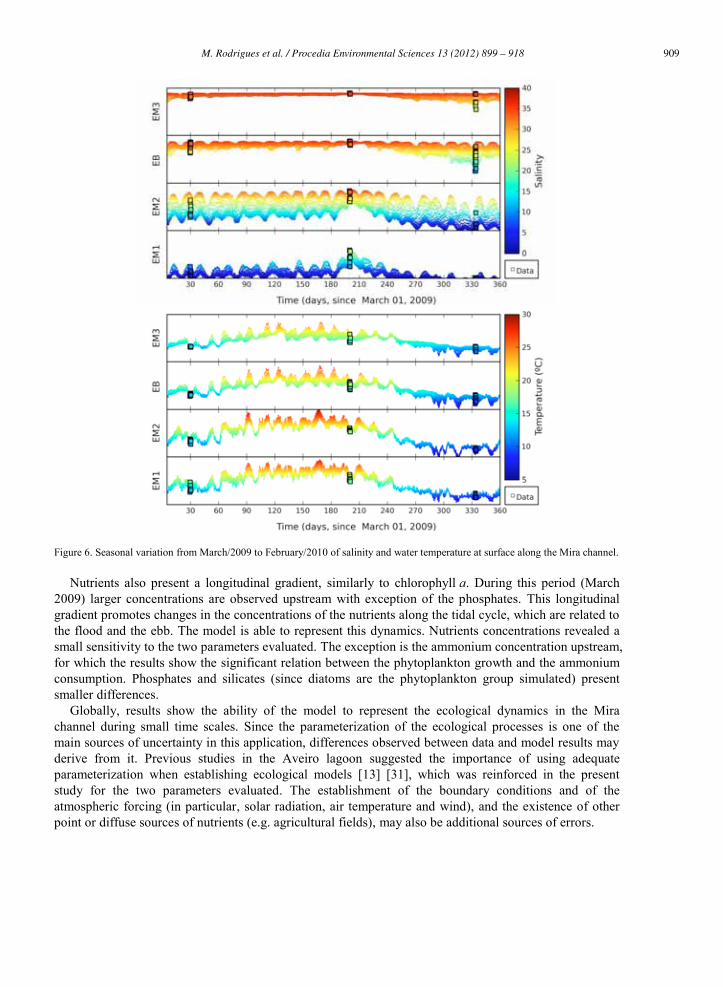
A longitudinal gradient of salinity is observed along the channel, varying from 36 downstream to almost 0 upstream during the wet season (Figures 5 and 6). During the tidal cycle salinity variations are observed along the channel: during flood, salinity increases upstream, while it decreases during ebb downstream. The larger salinity variations are observed at station EM2. Seasonally larger amplitudes are observed during the wet periods, when the river flows are larger. During winter, salinities near the downstream area of the channel (station EB and EM3) can reach values smaller than 20. During the dry season, salinity variations in the tidal cycle are smaller and increase in the upstream station (EM1) to values of about 20. No significant stratification is observed along the channel (results not shown). The model is able to represent both the tidal and the seasonal variations of salinity along the Mira channel with differences generally smaller than 2.5.

Water temperature also presents variations at both spatial and temporal scales (diurnal and seasonal). During the day, an increase of temperature is observed, which is more significant in the shallower areas located upstream in the channel (Figure 5). At the seasonal scale, water temperature varies from values of 20-30 ºC in the summer and decreases to 5-10 ºC in the winter. The model is also able to reproduce the temperature patterns observed, with differences smaller than 1 C.


a) b)

Figure 4. Comparison between data and model results: (a) water level variation at station EM3 and (b) velocity at station EB (positive values represent flood).

Figure 5. Diurnal variation (March 29-30, 2009) of salinity and water temperature at surface along Mira channel.

5.2. Diurnal variability of ecological tracers

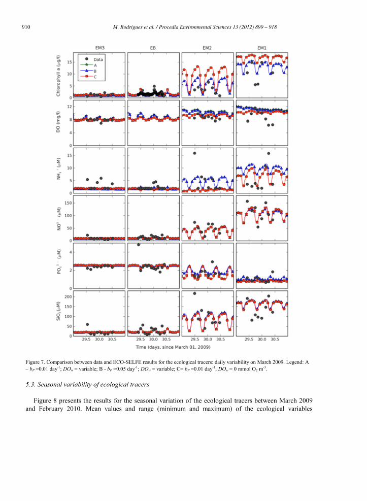
Results for the diurnal variability of ecological tracers on March 2009 are presented in Figure 7. Chlorophyll a presents a longitudinal gradient along the channel, decreasing from upstream

(5-15 g l-1) to downstream (<2 g l-1). The model is able to represent this gradient, in particular for the phytoplankton basal specific respiration rate of 0.045 day-1. During the night (day 30) an increase of the chlorophyll a concentrations is observed downstream, which is related with the tidal cycle and the transport during the ebb of the upstream water masses that present larger concentrations.

Dissolved oxygen longitudinal and diurnal variations are relatively smaller, with exception of the EM1 station (Areão) where a decrease of 3-4 mg l-1 is observed during the night. The model is able to represent the main patterns observed with differences smaller than 1 mg/l. At the EM1 station previous studies showed a similar pattern in the dissolved oxygen diurnal variation, which was explained by the photosynthetic and respiration dynamics of the vegetation that covers the channel bed [31]. Thus, the differences observed between the data and the model in this station may derive from the fact that only the lower trophic levels dynamics is represented by the model. The effect of the increase in oxygen saturation concentration due to the wind is observed only in this tracer and is more significant in the shallower areas of the lagoon (stations EM2 and EM1).


Figure 6. Seasonal variation from March/2009 to February/2010 of salinity and water temperature at surface along the Mira channel.

Nutrients also present a longitudinal gradient, similarly to chlorophyll a. During this period (March 2009) larger concentrations are observed upstream with exception of the phosphates. This longitudinal gradient promotes changes in the concentrations of the nutrients along the tidal cycle, which are related to the flood and the ebb. The model is able to represent this dynamics. Nutrients concentrations revealed a small sensitivity to the two parameters evaluated. The exception is the ammonium concentration upstream, for which the results show the significant relation between the phytoplankton growth and the ammonium consumption. Phosphates and silicates (since diatoms are the phytoplankton group simulated) present smaller differences.

Globally, results show the ability of the model to represent the ecological dynamics in the Mira channel during small time scales. Since the parameterization of the ecological processes is one of the main sources of uncertainty in this application, differences observed between data and model results may derive from it. Previous studies in the Aveiro lagoon suggested the importance of using adequate parameterization when establishing ecological models [13] [31], which was reinforced in the present study for the two parameters evaluated. The establishment of the boundary conditions and of the atmospheric forcing (in particular, solar radiation, air temperature and wind), and the existence of other point or diffuse sources of nutrients (e.g. agricultural fields), may also be additional sources of errors.


Figure 7. Comparison between data and ECO-SELFE results for the ecological tracers: daily variability on March 2009. Legend: A – bP =0.01 day-1; DOw = variable; B - bP =0.05 day-1; DOw = variable; C= bP =0.01 day-1; DOw = 0 mmol O2 m-3.

5.3. Seasonal variability of ecological tracers

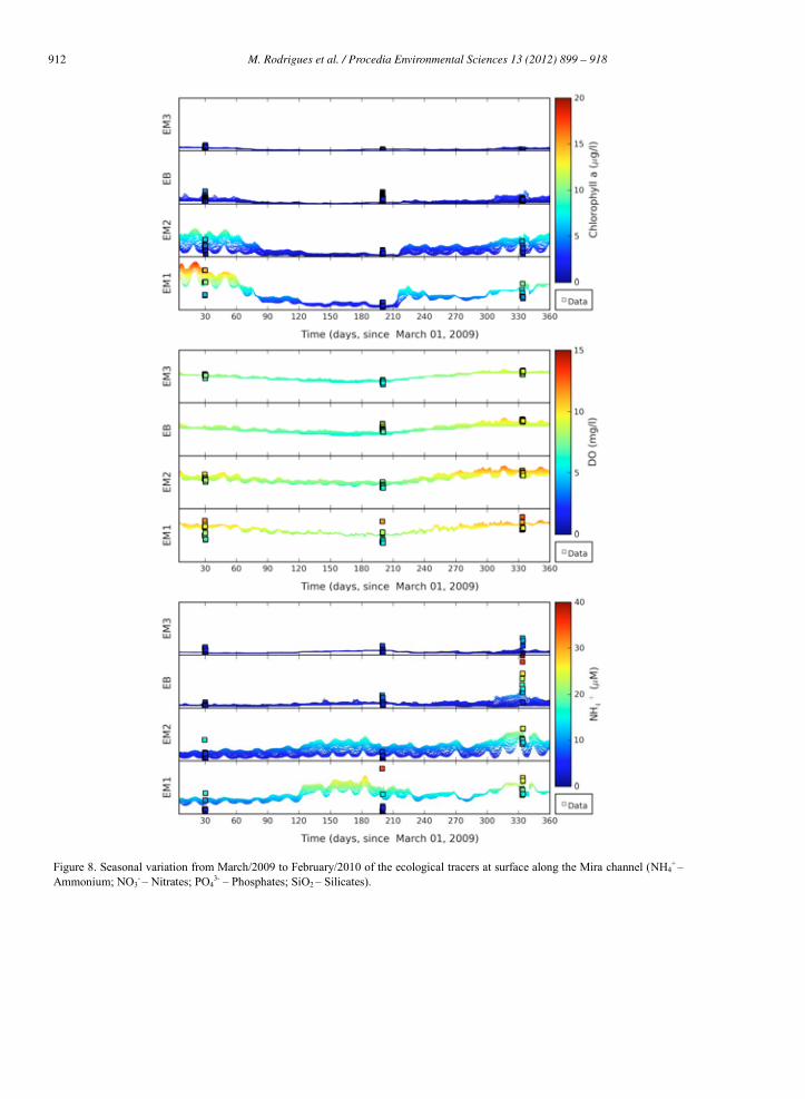
Figure 8 presents the results for the seasonal variation of the ecological tracers between March 2009 and February 2010. Mean values and range (minimum and maximum) of the ecological variables


measured during each field campaign and a comparison with model results for the same periods are presented in Table 2.

Chlorophyll a showed a seasonal pattern, in particular, at the upstream stations (EM1 and EM2). At station EM3, concentrations remained bellow 1 g l-1 almost during the entire year. At the upstream stations larger concentrations were observed in Spring (March 2009), where chlorophyll a ranged from 0.9 g l-1 to 18.9 g l-1 (mean values of 10.3 g l-1 and 4.0 g l-1 at station EM1 and EM2, respectively). At station EM1 chlorophyll a concentrations reached values of 6.0 g l-1 (2.6-10.0 g l-1) on January 2010, which are larger than the ones observed on September 2009. Larger concentrations of chlorophyll a had already been observed by [32] during winter in the upstream end of Mira channel. Vertically, differences in the water column were usually smaller than 0.5-1.0 g l-1; some exceptions were observed at station EM1 on March 2009 and at station EM3 on September 2009 (results not shown). The model is able to represent the main patterns observed in the seasonal variation of chlorophyll a along the channel with mean differences generally smaller than 1-2 g l-1. The differences observed between the data and the model results may be related with the sources of errors identified previously (section 5.2), in particular those related to the boundary conditions, the atmospheric forcing and the uncertainty in the parameterization. [33] identified a seasonal succession of phytoplankton in the Aveiro lagoon dominated by diatoms from late autumn until early spring, and by chlorophytes during late spring and summer. Since only one group of phytoplankton is considered in the simulations, this may also explain some of the differences observed. However increasing the number of phytoplankton groups would increase the uncertainty in the parameterization of the ecological model.

Dissolved oxygen varied seasonally in about 4 mg l-1. Smaller concentrations, of about 6-7 mg l-1, were observed during the summer (September 2009), while larger concentrations, of about 9-10 mg l-1, were observed during the winter (January 2010). This seasonal pattern was common along the channel. At EM1 station (Areão) the diurnal variation of the dissolved oxygen concentration was observed during the three campaigns, with a significant decrease during the night. At this station, the model is able to represent the mean values observed, with differences smaller than 1.3 mg l-1, but fails the full range of amplitude observed, as discussed previously (section 5.2). At the other stations (EM2, EM3 and EB) differences between the data and the model are usually smaller than 1 mg l-1 during the entire period simulated. Due to the influence of the wind in the dissolved oxygen concentration some of the differences observed may also derive of the wind forcing that was considered spatially constant, based on the data available (Figure 9). Regarding vertical variations in the water column data showed that concentrations tend to be slightly larger at the surface, due to the exchanges between the water and the atmosphere, however these differences are small (Figure 10).

Ammonium presented a seasonal pattern that was more significant upstream. At station EM1 mean concentrations ranged from 4.3 M during spring (March 2009) to the largest value of about 20 M in the winter (January 2010). At the downstream station EM3 the range of variation was smaller (3.1-4.2 M). The increase observed in ammonium concentrations during the winter is associated with less consumption by phytoplankton cells during this period. Although some occasional differences were observed through the water column, the vertical variation was small (results not shown). Globally, the model represents the mean patterns of ammonium both at the seasonal scale and longitudinally along the channel. The main differences are observed in the range of variation, the model failing to represent some of the maximum concentrations measured occasionally. This may be related to some discharges, to variations at the boundaries (where concentration was held constant monthly) or to sediments ressuspension. In January 2010 data also showed an increase on ammonium concentrations at the EB station, that was not observed at the other stations and may indicate a point source or discharge that is not considered in the model.


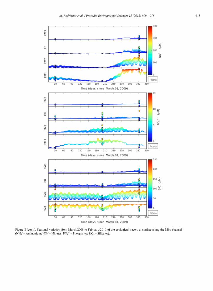
Figure 8. Seasonal variation from March/2009 to February/2010 of the ecological tracers at surface along the Mira channel (NH4+ –

Ammonium; NO3- – Nitrates; PO4

3- – Phosphates; SiO2 – Silicates).


Figure 8 (cont.). Seasonal variation from March/2009 to February/2010 of the ecological tracers at surface along the Mira channel (NH4

+ – Ammonium; NO3- – Nitrates; PO4

3- – Phosphates; SiO2 – Silicates).


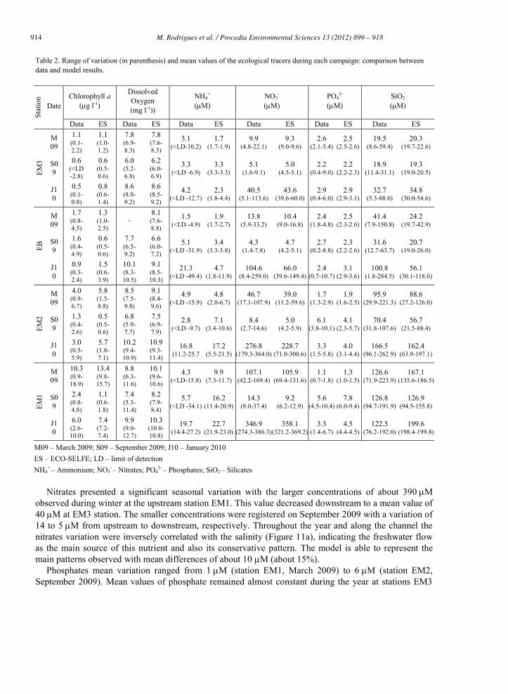
Table 2. Range of variation (in parenthesis) and mean values of the ecological tracers during each campaign: comparison between data and model results.

Stat

ion

Date Chlorophyll a

(g l-1)

Dissolved Oxygen (mg l-1))

NH4+

(M) NO3

- (M)

PO43-

(M) SiO2 (M)

Data ES Data ES Data ES Data ES Data ES Data ES

EM3

M09

1.1 (0.1-2.2)

1.1 (1.0-1.2)

7.8 (6.9-8.3)

7.8 (7.6-8.3)

3.1 (<LD-10.2)

1.7 (1.7-1.9)

9.9 (4.8-22.1)

9.3 (9.0-9.6)

2.6 (2.1-5.4)

2.5 (2.5-2.6)

19.5 (8.6-59.4)

20.3 (19.7-22.6)

S09

0.6 (<LD-2.8)

0.6 (0.5-0.6)

6.0 (5.2-6.8)

6.2 (6.0-6.9)

3.3 (<LD -6.9)

3.3 (3.3-3.3)

5.1 (1.6-9.1)

5.0 (4.5-5.1)

2.2 (0.4-9.0)

2.2 (2.2-2.3)

18.9 (11.4-31.1)

19.3 (19.0-20.5)

J10

0.5 (0.1-0.8)

0.8 (0.6-1.4)

8.6 (8.0-9.2)

8.6 (8.5-9.2)

4.2 (<LD -12.7)

2.3 (1.8-4.4)

40.5 (5.1-113.6)

43.6 (39.6-60.0)

2.9 (0.4-6.0)

2.9 (2.9-3.1)

32.7 (5.3-88.0)

34.8 (30.0-54.6)

EB

M09

1.7 (0.8-4.5)

1.3 (1.0-2.5)

- 8.1 (7.6-8.8)

1.5 (<LD -4.9)

1.9 (1.7-2.7)

13.8 (5.9-33.2)

10.4 (9.0-16.8)

2.4 (1.8-4.8)

2.5 (2.3-2.6)

41.4 (7.9-150.8)

24.2 (19.7-42.9)

S09

1.6 (0.4-4.9)

0.6 (0.5-0.6)

7.7 (6.5-9.2)

6.6 (6.0-7.2)

5.1 (<LD -31.9)

3.4 (3.3-3.8)

4.3 (1.4-7.8)

4.7 (4.2-5.1)

2.7 (0.2-8.8)

2.3 (2.2-2.6)

31.6 (12.7-63.7)

20.7 (19.0-26.0)

J10

0.9 (0.3-2.4)

1.5 (0.6-3.9)

10.1 (8.3-10.5)

9.1 (8.5-10.3)

21.3 (<LD -49.4)

4.7 (1.8-11.9)

104.6 (8.4-259.0)

66.0 (39.6-149.4)

2.4 (0.7-10.7)

3.1 (2.9-3.6)

100.8 (1.8-284.5)

56.1 (30.1-118.0)

EM2

M09

4.0 (0.9-6.7)

5.8 (1.5-8.8)

8.5 (7.5-9.8)

9.1 (8.4-9.6)

4.9 (<LD -15.9)

4.8 (2.0-6.7)

46.7 (17.1-107.9)

39.0 (11.2-59.6)

1.7 (1.3-2.9)

1.9 (1.6-2.5)

95.9 (29.9-221.3)

88.6 (27.2-126.0)

S09

1.3 (0.4-2.6)

0.5 (0.5-0.6)

6.8 (5.9-7.7)

7.5 (6.9-7.9)

2.8 (<LD -9.7)

7.1 (3.4-10.6)

8.4 (2.7-14.6)

5.0 (4.2-5.9)

6.1 (3.8-10.1)

4.1 (2.3-5.7)

70.4 (31.8-107.6)

56.7 (21.5-88.4)

J10

3.0 (0.5-5.9)

5.7 (1.8-7.1)

10.2 (9.4-10.9)

10.9 (9.3-11.4)

16.8 (11.2-25.7

17.2 (5.5-21.5)

276.8 (179.3-364.0)

228.7 (71.0-300.6)

3.3 (1.5-5.8)

4.0 (3.1-4.4)

166.5 (96.1-262.9)

162.4 (63.9-197.1)

EM1

M09

10.3 (0.9-18.9)

13.4 (9.8-15.7)

8.8 (6.3-11.6)

10.1 (9.6-10.6)

4.3 (<LD-15.8)

9.9 (7.3-11.7)

107.1 (42.2-169.4)

105.9 (69.4-131.6)

1.1 (0.7-1.8)

1.3 (1.0-1.5)

126.6 (71.9-223.9)

167.1 (135.6-186.5)

S09

2.4 (0.8-4.8)

1.1 (0.6-1.8)

7.4 (5.3-11.4)

8.2 (7.9-8.4)

5.7 (<LD -34.1)

16.2 (11.4-20.9)

14.3 (8.0-37.4)

9.2 (6.2-12.9)

5.6 (4.5-10.4)

7.8 (6.0-9.4)

126.8 (94.7-191.9)

126.9 (94.5-155.8)

J10

6.0 (2.6-10.0)

7.4 (7.2-7.4)

9.9 (9.0-12.7)

10.3 (10.0-10.8)

19.7 (14.4-27.2)

22.7 (21.9-23.0)

346.9 (274.3-386.3)

358.1 (321.2-369.2)

3.3 (1.4-6.7)

4.5 (4.4-4.5)

122.5 (76.2-192.0)

199.6 (198.4-199.8)

M09 – March 2009; S09 – September 2009; J10 – January 2010 ES – ECO-SELFE; LD – limit of detection NH4

+ – Ammonium; NO3- – Nitrates; PO4

3- – Phosphates; SiO2 – Silicates

Nitrates presented a significant seasonal variation with the larger concentrations of about 390 M

observed during winter at the upstream station EM1. This value decreased downstream to a mean value of 40 M at EM3 station. The smaller concentrations were registered on September 2009 with a variation of 14 to 5 M from upstream to downstream, respectively. Throughout the year and along the channel the nitrates variation were inversely correlated with the salinity (Figure 11a), indicating the freshwater flow as the main source of this nutrient and also its conservative pattern. The model is able to represent the main patterns observed with mean differences of about 10 M (about 15%).

Phosphates mean variation ranged from 1 M (station EM1, March 2009) to 6 M (station EM2, September 2009). Mean values of phosphate remained almost constant during the year at stations EM3


and EB (2-3 M), while at stations EM1 and EM2 a seasonal variation, with larger concentrations on September 2009, was observed. On September 2009 larger concentrations of phosphates were also observed at the surface samples of the station EB, which may be related to sediments ressuspension. During this period the model is not able to represent the vertical variation observed, since the exchanges between the sediments and the water column are not implemented in the model. As for ammonium, the model also lacks the representation of some occasional larger concentrations. In terms of mean variation the differences between the data and the model results are generally smaller than 1-2 M.

Figure 9. Wind intensity from March 2009 to February 2010: hourly and mean monthly values.

Figure 10. Vertical variation (surface and bottom) of dissolved oxygen at station EM2 (March 2009) and station EM3 (January 2010).

a) b)

Figure 11. Correlation between salinity and: a) nitrates and b) silicates concentrations (r – Pearson correlation coefficient; values are presented only for stations EM1, EM2 and EM3).

Silicates presented larger concentrations during the winter (January 2011), except at station EM1 where mean concentrations remained approximately constants (about 125 M). As nitrates, silicates are also inversely correlated with the salinity (Figure 11b), as their main sources are precipitation and flood


events [35]. However, at station EM2 during the winter (January 2010) the diurnal variation observed was not related with the tide, but probably was due to sediment ressuspension. Globally the model represents the several patterns observed for this variable. The main differences observed may derive from the aspects mentioned above for the other nutrients.

6. Conclusions

ECO-SELFE, a fully coupled hydrodynamic and ecological model, was extended for the oxygen cycle simulation and validated at diurnal and seasonal time scales along the Mira channel in the Aveiro lagoon. Validation was performed against a set of data collected specifically for this effect, contributing the combined analysis of the data and model results to an improvement on the knowledge of this system variability.

Results showed that the coupled model is able to represent the main patterns of the physical, chemical and ecological processes along the channel, for the different time scales evaluated. The differences observed are, generally, smaller or similar to the ones achieved in this type of modelling applications (e.g. [12][36]). The diurnal variability observed is mostly associated with the tide. Freshwater from upstream (usually with larger concentrations of chlorophyll a and nutrients) is transported downstream during the ebb. Seasonally the variations are associated with the river flow and the variation of the concentrations at the boundaries, and also with the atmospheric variations.

The main differences observed between the data and the model results may derive from three main factors. First, the parametrization of the ecological processes, which is simultaneously one of the most important steps and one of the main sources of uncertainty in the application of this type of models. Second, the sources flowing to the system and, in particular, the uncertainty in the establishment of the boundary conditions, since a continuous monitoring strategy does not exist in this system. The existence of additional, unknown point or diffuse sources that are not considered in the model may also explain the differences observed. Third, the existence of other processes that are not implemented in the model, namely the ressuspension of the sediments, and may contribute to changes in the concentrations observed in the water column.

Results also showed the importance of establishing adequate monitoring campaigns with periodicity and spatial coverage that allow the validation of ecological models at the scales of interest.

Globally, ECO-SELFE extension and validation showed its utility and applicability as a tool to support the management of the estuarine ecosystems and, in particular, to study the impacts of climate changes and anthropogenic pressures in the water quality and ecological dynamics of the Aveiro lagoon.

Acknowledgements

The first author is partly funded by Fundação para a Ciência e Tecnologia (FCT) grant SFRH/BD/41033/2007. This work was partly funded by the FCT project GCast (GRID/GRI/81733/2006) and Fundação Luso Americana para o Desenvolvimento project BGEM. The field and the laboratorial work had the participation of: M. Guerreiro, A. Azevedo, X. Bertin, A. Nahon, N. Bruneau, A. Ré, R. Marques, A. Pereira, B. Silva, S. Tavares, J. Carvalho, J. Dias, S. Plecha T. Diniz, C. Sá and F. Santos. The authors also thank Prof.ª Maria Dolores Manso the data from the University of Aveiro meteorological station, Prof. Joseph Zhang and Prof. António Melo Baptista for making SELFE code available and Doctor Alberto Azevedo for the post-processing code. The NCEP Reanalysis data is provided by the NOAA/OAR/ESRL PSD, Boulder, Colorado, USA, from their Web site at http://www.esrl.noaa.gov/psd/.


References

[1] Lopes JF, Dias JM, Cardoso AC, Silva CIV. The water quality of the Ria de Aveiro lagoon, Portugal: From the observations to the implementation of a numerical model. Mar Environ Res 2005;60:594-628.

[2] Gameiro C, Brotas V. Patterns of phytoplankton variability in Tagus Estuary (Portugal). Estuar Coast Special Issue: Phytoplankton in Coastal Ecosystems 2010;33:311-23.

[3] Intergovernamental Panel on Climate Changes. Climate Change 2007: The Physical Science Basis. UNEP and WMO, 2007 (http://www.ipcc.ch/SPM2feb07.pdf).

[4] Hays, GC, Richardson, AJ, Robinson, C. Climate change and marine plankton. Trends Ecol Evol 2005; 20(6):337-334. [5] Smith W, Steinberg D, Bronk D, Tang K. Marine plankton food webs and climate change. Virginia Institute of Marine

Science, 2008. [6] Grant SB, Kim JH, Jones BH, Jenkins SA, Wasyl J, Cudaback C. Surf zone entrainment, along-shore transport and human

health implication of pollution from tidal inlets. J Geophys Res 2005;110(C10025):1-20. [7] Bisset WP, Debra S, Dye D. Ecological Simulation (EcoSim) 2.0 Technical Description, Tampa, Florida: Florida

Environmental Research Institute, 2004. [8] Baretta-Bekker JG, Baretta JW. European Regional Seas Ecosystem Model (ERSEM II). J Sea Res 1997; 38:169-438. [9] Kishi MJ, Kashiwai M, Ware DM, Megrey BA, Eslinger DL, Werner FE, Noguchi-Aita M, Azumaya T, Fujii M, Hashimoto

S, Huang D, Iizumi H, Ishida Y, Kang S, Kantakov GA, Kim H, Komatsu K, Navrotsky VV, Smith SL, Tadokoro K, Tsuda A, Yamamura O, Yamanaka Y, Yokouchi K, Yoshie N, Zhang J, Zuenko YI, Zvalinsky ZI. NEMURO – a lower trophic level model for the North Pacific marine ecosystem. Ecol Model 2007;202:12-25.

[10] Trancoso AR, Saraiva S, Fernandes L, Pina P, Leitão P, Neves R. Modelling macroalgae using a 3D hydrodynamic-ecological model in a shallow, temperate estuary. Ecol Model 2005;187:232–46.

[11] Lopes JF, Dias JM, Dekeyser I. Numerical modelling of cohesive sediments transport in the Ria de Aveiro lagoon. J Hydrol 2006;319(1-4):176-98.

[12] Lopes JF, Silva CI, Cardoso AC. Validation of a water quality model for the Ria de Aveiro lagoon, Portugal. Environ Modell Softw 2008;23:479-94.

[13] Rodrigues M, Oliveira A, Queiroga H, Fortunato AB, Zhang YJ. Three-dimensional modeling of the lower trophic levels in the Ria de Aveiro. Ecol Model 2009;220(9-10):1274-90.

[14] Dias JM, Lopes JF. Implementation and assessment of hydrodynamic, salt and heat transport models: the case of Ria de Aveiro lagoon (Portugal). Environ Modell Softw 2006;21:1-15.

[15] Dias JM, Lopes JF, Dekeyser I. Tidal propagation in Ria de Aveiro lagoon, Portugal. Phys Chem Earth 2000;25:369-74. [16] Dias JM, Lopes JF, Dekeyser I. Lagrangian transport of particles in Ria de Aveiro lagoon, Portugal. Phys Chem Earth, Part

B: Hydrology, Oceans and Atmosphere 2001;26(9):721-7. [17] Lorezen CJ. Determination of chlorophyll and phaeopigments: spectrophotometric equations. Limnol Oceanogr

1967;12(2):343–6. [18] Koroleff F. Direct determination of ammonia in natural water as indophenol blue. ICES, Pap. C.M. 1969/C:9, revised 1970,

19-22. [19] Grasshoff K. Methods of seawater analysis, Verlag, NY: Chimie; 1976. [20] Murphy J, Riley JP. A modified single solution method for the determination of phosphate in natural waters. Chimie Acta

1962,27:301-18. [21] Famming JC, Pilson MEQ. On the spectrophotometric determination of dissolved silica in natural waters. Anal Chem

1973;45:136-40. [22] Zhang Y, Baptista AM. SELFE: A semi-implicit Eulerian-Lagrangian finite-element model for cross-scale ocean circulation.

Ocean Model 2008;21(3-4):71-96. [23] Rodrigues M, Oliveira A, Queiroga H, Zhang YJ, Fortunato AB, Baptista AM. Integrating a circulation model and an

ecological model to simulate the dynamics of zooplankton. In: Spaulding M, editors. Estuarine and Coastal Modeling Conference Book, Proceedings of the Tenth International Conference, New York: ASCE; 2008, p. 427-46.


[24] Vichi M, Pinardi N, Masina S. A generalized model of pelagic biogeochemistry for the global ocean ecosystem. Part I: Theory. J Mar Syst 2007;64:89-109.

[25] Hull V, Parrella L, Falcucci M. Modelling dissolved oxygen in coastal lagoons. Ecol Model 2008;211:468-80. [26] Thomann, RV, Mueller JA. Principles of surface water quality modeling and control. New York: Harper and Row

Publishing; 1987. [27] Wanninkhof R. Relationship between wind speed and gas exchange over the ocean. J Geophys Res 1992;97(C5):7373-82. [28] Weiss RF. The solubility of nitrogen, oxygen and argon in water and seawater. Deep Sea Res 1970;17:721-35. [29] Fortunato AB, Pinto LL, Oliveira A, Ferreira JS. Tidally-generated shelf waves off the western Iberian coast. Cont Shelf

Res 2002;22(14):1935-50. [30] Zeng X, Zhao M, Dickinson RE. Intercomparison of bulk aerodynamic algorithms for the computation of sea surface fluxes

using TOGA COARE and TAO data. J Climate 1998; 11:2628-44. [31] Rodrigues M, Oliveira A, Costa M, Fortunato AB, Zhang YJ. Sensitivity analysis of an ecological model applied to the Ria

de Aveiro. J Coastal Res 2009;SI56:448-52. [32] Fujii M, Yamanaka Y, Nojiri Y, Kishi MJ, Chai F. Comparison of seasonal characteristics in biogeochesmitry among the

subartic North Pacific stations described with a NEMURO-based ecosystem model. Ecol Model 2007;202:52-67. [33] Cunha MR, Moreira MH. Macrobenthos of potamogetonand myriophyllumbeds in the upper reaches of canal de Mira (Ria

de Aveiro, NW Portugal): community structure and environmental factors. Neth J Aquat Ecol 1995;29(3-4):377-90. [34] Leandro SM. Forçamento ambiental na abundância e produção de zooplâncton num gradiente estuarino. PhD Thesis,

Universidade de Aveiro, 2008. [35] Lopes CB, Lillebo AI, Dias JM, Pereira E, Vale C, Duarte AC. Nutrient dynamics and seasonal succession of

phytoplankton assemblages in a southern european estuary: Ria de Aveiro, Portugal. Estuar Coast Shelf S 2007;71:480-90. [36] Fitzpatrick JJ. Assessing skill of estuarine and coastal eutrophication models for water quality managers. J Marine Syst

2009;76:195-211.

Seasonal and diurnal water quality and ecological dynamics along … · 2017-01-20 · valuable...

Documents

Transcript of Seasonal and diurnal water quality and ecological dynamics along … · 2017-01-20 · valuable...