Draft version June 28, 2021Typeset using LATEX twocolumn style in AASTeX63

Searching For Transiting Planets Around Halo Stars. I. Sample Selection and Validation

Jared R. Kolecki,1 Ji Wang (王吉) ,1 Jennifer A. Johnson,1 Joel C. Zinn,1, 2, ∗ Ilya Ilyin,3 andKlaus G. Strassmeier3

1Department of Astronomy, The Ohio State University, Columbus, Ohio 43210, USA2Department of Astrophysics, American Museum of Natural History, Central Park West at 79th Street, New York, NY 10024, USA

3Leibniz-Institute for Astrophysics Potsdam (AIP), An der Sternwarte 16, D-14482 Potsdam, Germany

(Received January 18, 2021; Revised May, June 2021; Accepted June 28, 2021)

Submitted to AJ

ABSTRACT

By measuring the elemental abundances of a star, we can gain insight into the composition of its

initial gas cloud—the formation site of the star and its planets. Planet formation requires metals,

the availability of which is determined by the elemental abundance. In the case where metals are

extremely deficient, planet formation can be stifled. To investigate such a scenario requires a large

sample of metal-poor stars and a search for planets therein. This paper focuses on the selection and

validation of a halo star sample. We select ∼17,000 metal-poor halo stars based on their Galactic

kinematics, and confirm their low metallicities ([Fe/H] < −0.5), using spectroscopy from the literature.

Furthermore, we perform high-resolution spectroscopic observations using LBT/PEPSI and conduct

detailed metallicity ([Fe/H]) analyses on a sample of 13 previously known halo stars that also have

hot kinematics. We can use the halo star sample presented here to measure the frequency of planets

and to test planet formation in extremely metal-poor environments. The result of the planet search

and its implications will be presented and discussed in a companion paper by Boley et al.

Keywords: Halo stars, Exoplanets, Metallicity

1. INTRODUCTION

When and under what conditions did the first planet

form? The oldest planetary system that we know of is

∼11.2 Gyr old (Kepler-444, Campante et al. 2015; Mack

et al. 2018), with a host star metallicity of [Fe/H] =

−0.52. The first generation of stars and planets is ex-

pected to have metallicities similar to or below that

of Kepler-444. Such a metal-poor environment poses

challenges for planet formation. For gas giant planets,

core mass growth via accretion halts in the extremely

metal-poor regime, resulting in a strong dependence of

planet occurrence rate on stellar metallicity—known as

the planet-metallicity correlation (e.g., Fischer & Valenti

2005). For terrestrial planets, the planet-metallicity cor-

relation is weaker (Wang & Fischer 2015) and period-

dependent (Wilson et al. 2018; Petigura et al. 2018).

Therefore, metallicity is a key to regulate planet for-

∗ NSF Astronomy and Astrophysics Postdoctoral Fellow.

mation. More interestingly, some elements (e.g., α-

elements) may play a bigger role than others (Adibekyan

et al. 2012; Bashi & Zucker 2019).

The abundance of the elements increases as the MilkyWay evolves. Among the stellar populations in the

Milky Way, halo stars are the most metal-poor on av-

erage and therefore serve as an ideal test ground for

planet formation in metal-poor environments. However,

identifying halo stars is difficult because halo stars are

relatively rare in the solar neighborhood, representing

of order 1% of the local population; discovering them

has historically been laborious; and detailed character-

ization via high-resolution spectroscopy has been time-

consuming (see Carney & Latham (1987) and associated

works).

The Gaia mission (Gaia Collaboration et al. 2016) sig-

nificantly changed the landscape of the study of halo

stars, because we can use it to identify metal-poor stars

based on their kinematics, thanks to the well-known cor-

relation between the two (Eggen et al. 1962). Gaia’s as-

trometric and radial velocity measurements of one bil-

arX

iv:2

106.

1325

1v1

[as

tro-

ph.E

P] 2

4 Ju

n 20

21

2 Kolecki et al.

lion stars in the Milky Way provide an efficient way of

identifying halo stars. As such, we set out to iden-

tify stars with halo kinematics using the Gaia DR2

data (Gaia Collaboration et al. 2018). The kinematically

selected halo stars are then validated using data from the

APOGEE spectroscopic survey (Majewski et al. 2017)

and other photometric surveys to check the purity of the

sample.

Many of the halo stars are in the field of view of

the Transiting Exoplanet Survey Satellite (TESS, Ricker

et al. 2015). Searching for transiting planets around

halo stars are therefore made possible by the Gaia and

TESS missions. Our halo sample is much larger than

previous samples used for planetary searches via ra-

dial velocity (Sozzetti et al. 2006; Faria et al. 2016).

Since > 70% stars in our sample have [Fe/H]< −1,

our search will likely result in planetary systems that

are more metal-poor than the current record holder at

[Fe/H]=−0.84 (Anglada-Escude et al. 2014). The meth-

ods and results of the planet search are described in a

companion paper (Boley et al. 2021).

It is of interest to determine the absolute amount of

metal deficiency of the protoplanetary disk as input into

simulations of planet formation in disks (e.g., Johnson

& Li 2012). However, halo stars in the literature can

have values that differ by ∼ a factor of two, even when

all studies use high-resolution/high signal-to-noise data

(e.g., Jofre et al. 2014). Among the sources of systematic

differences in the studies, the validity of using ionization

equilibrium in LTE to determine gravity (Thevenin &

Idiart 1999) is another area where Gaia information is

crucial. Gaia parallaxes resolve the question of whether

a star is a subgiant or main-sequence star. We therefore

consider a selection of well-studied halo stars from the

literature with new spectra and analyses in this work.

The paper is organized as follows: Section 2 outlines

the process and criteria used to select a sufficiently pure

sample of halo dwarf stars, while Section 3 offers verifi-

cation of the success of the sample selection. Section 4

details the observation and data reduction process used

to generate the spectra used in Section 5 to analyze the

iron abundances of selected halo stars from the liter-

ature. The results of this analysis are discussed and

compared with other papers in Section 6.

2. SAMPLE SELECTION

Stars were selected preferentially from the CTLv0801

(Stassun et al. 2018, 2019) to have dwarf-like radii

(raddflag = 1); have Gaia DR2 parallaxes and proper

motions (PMFlag == ‘gaia2’; PARFlag == ‘gaia2’;

gaiaqflag == 1); be within 1kpc according to the

TICv8, which uses the Bailer-Jones et al. (2018) method

to calculate distance (Stassun et al. 2019) (this is to en-

sure that the kinematic cut described below is valid,

which was designed based on a simulation of the near-

est 1kpc stars); and be outside of the ecliptic plane

(|lat| > 6) to ensure candidates are observable by

TESS. Note that, although the majority of targets from

the CTL have T < 13, the Cool Dwarf list extends to

T = 16 (for a description of this special list, see Muir-

head et al. 2018).

Additional stars were selected by an equivalent search

in the TICv8 (Stassun et al. 2018, 2019) for stars with

13 ≤ T < 15 (otherwise the same cuts as for the CTL

are applied), effectively extending the magnitude limit

of the halo dwarf search to T < 15.

To select stars with halo-like kinematics, we ran a

Milky Way Galaxia (Sharma et al. 2011) simulation

of stars within 1kpc. We designed a kinematic cut to

choose halo stars based on only proper motion using

this simulation, so that a Gaia radial velocity was not

required. Our Galaxia simulations were run using the

default parameters, which are described in Sharma et al.

(2011). In particular, the Galaxia stellar halo geome-

try follows the Besancon model of an oblate spheroid,

with density proportional to(

Max(ac,a)R�

)n, where a2 =

R2 + z2

ε2 , ac = 500 pc, ε = 0.76, and n = −2.44 (Robin

et al. 2003), with R and z denoting Galactocentric cylin-

drical radius and height above the plane in pc. Following

Bond et al. (2010), the Galaxia halo velocity distribu-

tion is assumed to be an ellipsoid with σR = 141 km s−1

and σθ = σφ = 75 km s−1, which describes well the

observed SDSS halo velocity distribution within 10kpc

(Smith et al. 2009) as well that of Gaia halo stars (Posti

et al. 2018).

The resulting kinematic selection was applied to the

CTL/TIC sample, such that vδ < 0 km/s and ei-

ther vα < −230 km/s, vα > 210 km/s, or vδ <

−√

(1− ((vα + 10)× 220)2)× 230 km/s.

Finally, stars were selected to fall below the binary

sequence of a MIST 13 Gyr [Fe/H] = −1.0 (Dotter 2016;

Choi et al. 2016) isochrone in J − Ks–L space, where

the luminosity, L, is adopted from the TIC. The final

number of halo dwarf candidates selected in this way

is 16940. The stars passing the kinematic cuts versus

those passing the additional binary main sequence cut

are shown in Figure 1. An excerpt from the final sample

is displayed in Table 1. The entire catalog is available

electronically in csv format.

3. SAMPLE VALIDATION

Our sample selection can be tested by looking at the

subset of stars with full 3-D kinematics or with metallici-

ties. While the goal of the sample is to locate metal-poor

Transiting Planets Around Halo Stars I 3

Gaia DR2 ID pmRA (mas/yr) pmDEC (mas/yr) Tmag M/M� L/L� [M/H] from TIC

688442476835805312 66.074 -114.073 13.068 1.11 0.92 -1.52

800209689226496128 -234.096 -159.769 14.759 0.61 0.04 -1.11

1021587525024433152 -46.409 -55.106 14.499 1.26 0.59 -1.82

808143181016203264 60.511 -128.934 14.341 1.03 0.63 -1.43

Table 1. Selected entries from this paper’s final halo catalog. The entire catalog is available electronically asa csv file, featuring additional columns not present in this print version of the table.

0.2 0.4 0.6 0.8(J −Ks)0 [mag]

−2

0

2

Log 1

0Lu

min

osity

[L�

] KinematicKinematic+MS

Figure 1. Color-luminosity diagram demonstrating our H-R Diagram selection criteria. Dwarf halo candidates passingkinematic selection criteria are shown as a black contour,representing the 95% percentile. The binary main sequenceof a [Fe/H] = −1 isochrone is shown as the dashed curve, andthe distribution of the dwarf halo candidates falling belowthis sequence and therefore chosen as our final sample, isshown as the blue contour.

stars, confirming that the proper-motion selected stars

fall into kinematically hot populations when radial ve-

locities are added is also valuable, given the correlation

between the two properties.

3.1. Galactic Velocity Distribution

We calculated the Galactic space velocity (Johnson &

Soderblom 1987) for the 780 stars in the halo sample

that had available Gaia DR2 radial velocity data and

the 61 stars in the sample with APOGEE radial veloc-

ity data. Because radial velocity data are not used our

selection procedure, we can further verify the validity

of our selection with the galactic space velocity distri-

bution of the subsample with radial velocity data. The

Toomre diagram (Sandage & Fouts 1987) in Figure 2

shows that the galactic space velocities of these stars

are all above 200 km/s. We note that the distribution

is consistent with that from the literature that studied

metal-poor halo stars, which have Vtot > 180 km s−1

(e.g., Nissen & Schuster 2010; Schuster et al. 2012).

3.2. Metallicity Distribution

In addition to the 3-D kinematic verification of the

sample, we can also directly measure the degree to which

it is indeed metal-poor by appealing to independent

metallicities from the literature, which have been com-

piled by the TIC.

We analyzed the distribution of the TIC metallicities,

which are available for roughly 11% (n = 1,897) of the

sample, yielded an overall purity estimate of 70%, the

proportion of TIC metallicities which are below the low

metallicity threshold of [Fe/H] = 1.0. We note that

while the fraction of stars in the halo sample which have

TIC metallicities is relatively small, the roughly 2,000

data points available should provide a metallicity dis-

tribution which is sufficiently representative of that of

the entire halo sample. The distribution of these TIC

metallicities is shown in Figure 3.

It should be noted the metallicities in the TIC/CTL

are compiled from literature spectroscopic values, and

are therefore heterogeneous. In order of preference,

metallicities for the catalogue are adopted from: SPOCS

(Brewer et al. 2016); PASTEL (Soubiran et al. 2016);

Gaia-ESO DR3 (Gilmore et al. 2012); TESS-HERMES

DR1 (Sharma et al. 2018); GALAH DR2 (Buder et al.

2018); APOGEE-2 DR14 (Abolfathi et al. 2018); LAM-

OST DR4 (Luo et al. 2015); RAVE DR5 (Kunder et al.

2017); and Geneva-Copenhagen DR3 (Holmberg et al.

2009), as described in Stassun et al. (2019). While the

TIC metallicities may not be self-consistent and may

have a few tenths dex uncertainties, it provides a repre-

sentative distribution of the halo dwarf candidate sam-

ple metallicities.

4. OBSERVATIONS OF HALO STARS SHOWING

DISCREPANCIES IN STELLAR PROPERTIES

Some of our kinematically-selected halo stars have

been previously known and studied (Reddy et al. 2006;

Sozzetti et al. 2009; Boesgaard et al. 2011). However,

there are discrepancies in derived stellar properties such

as effective temperature and surface gravity, both among

the literature, and when the literature is compared to

the results of this paper. Table 2 shows effective tem-

4 Kolecki et al.

Figure 2. A projection of the stars’ 3-dimensional space velocity onto a 2-dimensional plane, where the x-axis representsvelocity in the direction of galactic rotation (V), and the y-axis represents the magnitude of the vector sum of radial velocity(U) and velocity perpendicular to the galactic plane (W). A star’s total velocity is represented by its distance from the originpoint (0,0). For this reason, iso-velocity lines are shown in gray for readability. All velocities are reported relative to the localstandard of rest. Error bars are approximately 3 km/s along either axis and thus are not visible on the scale of the plot.

Figure 3. The distribution of TIC metallicity values (n =1,897) of stars in the sample we selected. From the distri-bution, we estimate our complete sample to have a purity ofroughly 70%, as both distributions show 70% of their starshaving [Fe/H] < −1.0.

perature, surface gravity, and [Fe/H] values derived by

previous studies. Notable anomalies include the follow-

ing:

• BD+51 1696, the star measured by the greatest

number of studies we compared with, shows sig-

nificant spread in both Teff and log(g) between

studies.

• In many cases, Boesgaard et al. (2011) derives sur-

face gravities characteristic of post-main-sequence

stars, despite the selection process of this paperbeing designed to limit the sample to main se-

quence dwarfs.

This motivates us to observe 13 previously-known halo

stars using the PEPSI spectrograph (Strassmeier et al.

2015) at the Large Binocular Telescope (LBT, 2× 8.4 m

on Mt. Graham, Arizona, USA). The higher spectral

resolution (R=120,000) and a homogeneous abundance

analysis, in addition to the external constraints from the

Gaia DR2 data, help to reconcile the discrepancies and

lead to a more accurate determination of stellar proper-

ties. We detail the PEPSI observations and our abun-

dance measurements below.

LBT PEPSI observations were made on March 25,

May 15, June 23 and 25, 2019 UT with 200µm fiber

(R = 130 000 and 1.75′′ on sky) in two spectral regions

4800 - 5441 A and 6278 - 7419 A (cross-dispersers (CD) 3

Transiting Planets Around Halo Stars I 5

and 5) with 10–60 min integration time depending on the

star brightness. A typical signal-to-noise ratio achieved

is 350 in CD5 and 260 in CD3 for a star V=9.7 in one

hour integration time with two LBT mirrors. The whole

sample has signal-to-noise ratio ranging from 100 to 600.

4.1. Data Reduction

The data reduction is done using the Spectroscopic

Data Systems (SDS) with its pipeline adapted to the

PEPSI data calibration flow and image specific content.

Its description is given in Strassmeier et al. (2018).

The specific steps of image processing include bias

subtraction and variance estimation of the source im-

ages, super-master flat field correction for the CCD spa-

tial noise, echelle orders definition from the tracing flats,

scattered light subtraction, wavelength solution using

ThAr images, optimal extraction of image slices and

cosmic ray removal, wavelength calibration and merg-

ing slices in each order, normalization to the master flat

field spectrum to remove CCD fringes and blaze func-

tion, a global 2D fit to the continuum of the normalized

image, and rectification of all spectral orders in the im-

age to a 1D spectrum for a given cross-disperser.

The spectra from two sides of the telescope are aver-

aged with weights into one spectrum and corrected for

the barycentric velocity of the Solar system. The wave-

length scale is preserved for each pixel as given by the

wavelength solution without rebinning. The wavelength

solution uses about 3000 ThAr lines and has an uncer-

tainty of the fit at the image center of 4 m/s.

5. ABUNDANCE ANALYSIS

5.1. PEPSI spectra

To determine the metallicities and stellar parameters

of the stars observed with PEPSI, we first calculated

the equivalent widths (EW) of absorption lines in each

star’s spectrum. This was done using an automated pro-

gram which displays graphs and measurements from fits

of a Voigt and Gaussian distribution, along with its di-

rect measurement of the observed data. From this we

chose the method which most closely fit the data trend.

This manual screening allows for the best measurements

to be kept for all lines, mitigating the effects of noise,

contamination, and improper line fitting. If these ef-

fects are too great, the program allows us to discard the

measurement from the final data.

To streamline this process, if all three EW measure-

ments (Gaussian, Voigt, and raw) are within 20% of

each other, usually the result of a clean, isolated line

feature, the program automatically takes the average of

the three and uses the result as that line’s EW. On the

other hand, if both curve fitting functions fail, the line

is automatically discarded without prompting the user.

This latter scenario usually occurs where a line is weak

enough that it is completely drowned out by noise and

is indistinguishable from the continuum.

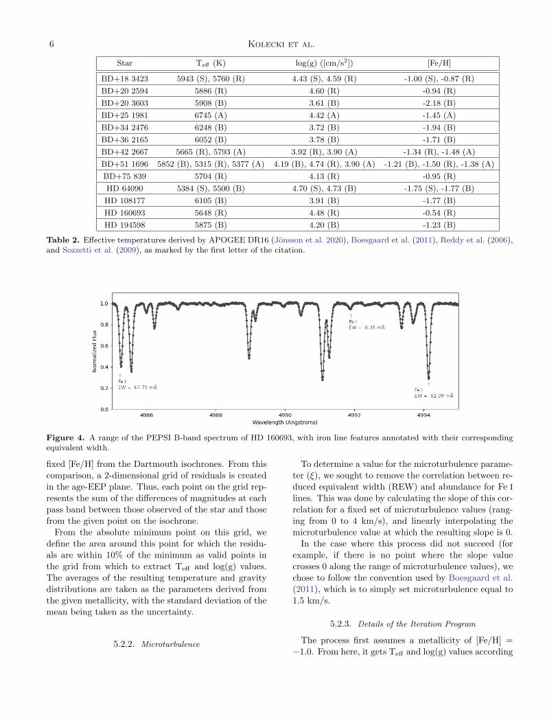
Line information was compiled from the NIST Atomic

Spectra Database (Kramida et al. 2020). A small sec-

tion of the PEPSI spectrum for the star HD 160693 is

shown in Figure 4 with line features annotated with their

corresponding species and equivalent width.

For each star, we chose to keep only lines for which

EW > 5m A, to minimize the effects of noise on weak

lines in our measurements. Furthermore, manual sigma-

clipping based on each individual line’s derived abun-

dance was performed after the initial analysis to remove

lingering outlying measurements, after which the pro-

cess was repeated. This was done twice. A complete list

of our final EW measurements can be found in Table 3.

5.2. Iterative MOOG Analysis

To derive abundances and stellar atmospheric pa-

rameters, we used a program written by the authors

which combines PyMOOGi1 (Adamow 2017), which is

a Python implementation of the Fortran code MOOG2

(Sneden 1973), with several Python functions designed

to iteratively derive stellar parameters, abundances, and

the uncertainties thereof.

We used the ATLAS9 model atmospheres computed

for the APOGEE survey (Meszaros et al. 2012), and

the PyKMOD atmosphere interpolator3 to create the

model stellar atmospheres for our analysis. To convert

the resulting abundance values into quantities relative to

solar, we took the solar iron abundance [Fe/H]� = 7.48

as stated in Palme et al. (2014).

5.2.1. Temperature and Surface Gravity

We used Gaia DR2 (Gaia Collaboration et al. 2018),

2MASS (Skrutskie et al. 2006), and WISE (Wright et al.

2010) photometry compared against Dartmouth theo-

retical isochrones4 (Dotter et al. 2007) to derive Teff and

log(g). The photometry was queried from its respective

databases using Astroquery, a module of the Astropy

software library (Price-Whelan et al. 2018). We used

distances computed by Bailer-Jones et al. (2018) to con-

vert these values from apparent to absolute magnitude.

The process is as follows: the star’s photometric pro-

file is compared against the synthetic photometry for

each age and equivalent evolutionary phase (EEP) at a

1 https://github.com/madamow/pymoogi2 http://www.as.utexas.edu/∼chris/moog.html3 https://github.com/kolecki4/PyKMOD4 http://stellar.dartmouth.edu/models/

6 Kolecki et al.

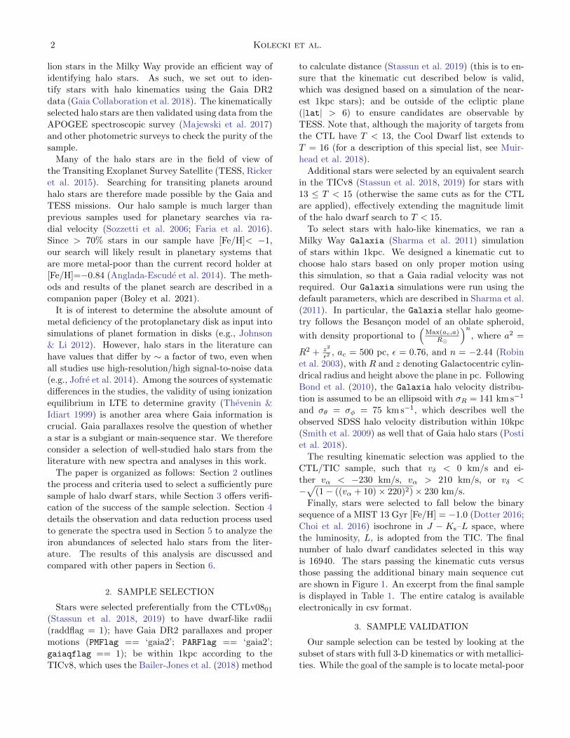
Star Teff (K) log(g) ([cm/s2]) [Fe/H]

BD+18 3423 5943 (S), 5760 (R) 4.43 (S), 4.59 (R) -1.00 (S), -0.87 (R)

BD+20 2594 5886 (R) 4.60 (R) -0.94 (R)

BD+20 3603 5908 (B) 3.61 (B) -2.18 (B)

BD+25 1981 6745 (A) 4.42 (A) -1.45 (A)

BD+34 2476 6248 (B) 3.72 (B) -1.94 (B)

BD+36 2165 6052 (B) 3.78 (B) -1.71 (B)

BD+42 2667 5665 (R), 5793 (A) 3.92 (R), 3.90 (A) -1.34 (R), -1.48 (A)

BD+51 1696 5852 (B), 5315 (R), 5377 (A) 4.19 (B), 4.74 (R), 3.90 (A) -1.21 (B), -1.50 (R), -1.38 (A)

BD+75 839 5704 (R) 4.13 (R) -0.95 (R)

HD 64090 5384 (S), 5500 (B) 4.70 (S), 4.73 (B) -1.75 (S), -1.77 (B)

HD 108177 6105 (B) 3.91 (B) -1.77 (B)

HD 160693 5648 (R) 4.48 (R) -0.54 (R)

HD 194598 5875 (B) 4.20 (B) -1.23 (B)

Table 2. Effective temperatures derived by APOGEE DR16 (Jonsson et al. 2020), Boesgaard et al. (2011), Reddy et al. (2006),and Sozzetti et al. (2009), as marked by the first letter of the citation.

Figure 4. A range of the PEPSI B-band spectrum of HD 160693, with iron line features annotated with their correspondingequivalent width.

fixed [Fe/H] from the Dartmouth isochrones. From this

comparison, a 2-dimensional grid of residuals is created

in the age-EEP plane. Thus, each point on the grid rep-

resents the sum of the differences of magnitudes at each

pass band between those observed of the star and those

from the given point on the isochrone.

From the absolute minimum point on this grid, we

define the area around this point for which the residu-

als are within 10% of the minimum as valid points in

the grid from which to extract Teff and log(g) values.

The averages of the resulting temperature and gravity

distributions are taken as the parameters derived from

the given metallicity, with the standard deviation of the

mean being taken as the uncertainty.

5.2.2. Microturbulence

To determine a value for the microturbulence parame-

ter (ξ), we sought to remove the correlation between re-

duced equivalent width (REW) and abundance for Fe I

lines. This was done by calculating the slope of this cor-

relation for a fixed set of microturbulence values (rang-

ing from 0 to 4 km/s), and linearly interpolating the

microturbulence value at which the resulting slope is 0.

In the case where this process did not succeed (for

example, if there is no point where the slope value

crosses 0 along the range of microturbulence values), we

chose to follow the convention used by Boesgaard et al.

(2011), which is to simply set microturbulence equal to

1.5 km/s.

5.2.3. Details of the Iteration Program

The process first assumes a metallicity of [Fe/H] =

−1.0. From here, it gets Teff and log(g) values according

Transiting Planets Around Halo Stars I 7

to Section 5.2.1, and interpolates a model atmosphere

from the grid with these photometric parameters and a

microturbulence set to 1.5 km/s. Then, it runs MOOG

with this model atmosphere and the line list for a given

star.

It then reads the MOOG output, gathering the metal-

licity data and a value for [Fe/H], and then repeats,

now using isochrones of the output [Fe/H] to derive new

parameters for the model atmosphere. Convergence is

reached and the process ends when the metallicity out-

put by MOOG is the same (to within 0.1 dex, the pre-

cision of the isochrone grid) as that used to derive that

run’s stellar parameters.

Note that the initial metallicity choice is arbitrary.

It is simply used as an initial guess for the iteration

process, which lasts a variable amount of time based on

how accurate this initial guess is.

After the process converges on a solution for [Fe/H],

we calculate the microturbulence as outlined in Section

5.2.2, re-deriving stellar parameters as necessary as the

microturbulence affects the metallicity. At this point,

the program proceeds with the uncertainty analysis.

5.3. Uncertainty Analysis

Uncertainty in the microturbulence parameter was de-

termined by perturbing the microturbulence until the

slope of the REW-abundance correlation fell outside of

the uncertainty range.

All other uncertainties, including those for Teff , log(g),

and abundances were calculated using iteration of the

process outlined in Section 3.2 of Epstein et al. (2010).

The method used by those authors creates a matrix of

partial derivatives of parameters with respect to one an-

other and uses various equations to account for the ef-

fects of uncertainties in each parameter on the uncer-

tainties of all the others.

Since, by the methodology outlined in Section 5.2.1,

the uncertainty in metallicity can affect the uncertainty

in Teff and log(g), and by the methodology outlined

here, the reverse is also true, we are required to iterate

these calculations repeatedly, using the output uncer-

tainties from one run as the input uncertainties of the

next.

Initial uncertainties were simply taken as the standard

deviation of the mean value derived for each parameter,

and the calculations taken from Epstein et al. were re-

peated until the [Fe/H] uncertainty was changed by less

than 0.01 dex from one iteration to the next.

5.4. Results

We found the stars to fall within a temperature range

of 5600 ≤ Teff ≤ 6800 and a surface gravity range of

4.1 ≤ log(g) ≤ 4.7. Detailed stellar parameter and

abundance results for each star can be found in Table 4.

The stars also fall well within the expected metallicity

values given their halo classification, as we found them

to fall within the range −2.0 < [Fe/H] < −0.6.

Figure 5. A plot of log(g) versus (G−Rp) color, overlayedwith isochrones of 6, 8, 10, and 12 Gyr for each metallicity.

6. DISCUSSION

6.1. Using Photometric vs Spectroscopic Parameters

One method of deriving stellar parameters involves

using the spectroscopic abundance analysis, adjusting

them until the following conditions are met:

1. Effective Temperature: The star should be in ex-

citation equilibrium, i.e. the correlation between abun-

dance derived from each line and excitation potential

(EP) should be removed.

2. Surface Gravity: The star should be in ionization

balance, i.e. the abundances of Fe I and Fe II should be

within 1σ of each other.

3. Microturbulence: There should be no correlation

between the abundance derived from each line and re-

duced equivalent width (log(EWλ )).

We followed this method for microturbulence, but our

Teff and log(g) values were derived photometrically from

isochrones. However, for every star except BD+75 839,

the resulting log(g) led to ionization balance.

Also, the resulting Teff led to excitation equilibrium

for many of the stars, such that the slope of the EP-

abundance regression line was equal to 0 at the 1-sigma

level for four stars, and at the 3-sigma for seven, where

sigma is defined as the standard deviation of the linear

regression fit assuming normal distribution of residuals.

Two stars (HD 64090 and HD 160693) featured slopes

which were 4-sigma away from zero. Notably however,

8 Kolecki et al.

Star Teff (K) log(g) ([cm/s2]) ξ (km/s) [Fe I/H] [Fe II/H]

BD+18 3423 6204 ± 70 4.19 ± 0.01 0.86 ± 0.21 -0.874 ± 0.099 -0.893 ± 0.103

BD+20 2594 6160 ± 40 4.29 ± 0.01 0.42 ± 0.29 -0.838 ± 0.067 -0.886 ± 0.079

BD+20 3603 6544 ± 20 4.32 ± 0.01 1.52 ± 0.28 -1.982 ± 0.116 -2.088 ± 0.140

BD+25 1981 6774 ± 20 4.18 ± 0.02 1.52 ± 0.24 -1.551 ± 0.140 -1.387 ± 0.150

BD+34 2476 6595 ± 40 4.11 ± 0.01 1.34 ± 0.21 -1.884 ± 0.110 -1.941 ± 0.145

BD+36 2165 6470 ± 20 4.19 ± 0.01 0.86 ± 0.23 -1.359 ± 0.053 -1.411 ± 0.046

BD+42 2667 6314 ± 30 4.32 ± 0.01 0.56 ± 0.27 -1.265 ± 0.086 -1.328 ± 0.091

BD+51 1696 5793 ± 20 4.57 ± 0.01 1.5 ± 0.71 -1.424 ± 0.084 -1.416 ± 0.096

BD+75 839 6320 ± 70 4.21 ± 0.05 1.10 ± 0.13 -0.769 ± 0.158 -1.151 ± 0.164

HD 64090 5607 ± 10 4.67 ± 0.01 1.5 ± 0.78 -1.650 ± 0.074 -1.846 ± 0.107

HD 108177 6410 ± 40 4.33 ± 0.01 0.59 ± 0.30 -1.479 ± 0.113 -1.502 ± 0.160

HD 160693 5951 ± 30 4.29 ± 0.01 1.5 ± 0.52 -0.610 ± 0.052 -0.613 ± 0.078

HD 194598 6243 ± 80 4.36 ± 0.02 1.5 ± 0.40 -1.131 ± 0.192 -1.243 ± 0.209

Table 4. Stellar Parameters of Selected Sample Stars

these two stars were also unable to achieve microturbu-

lence convergence.

6.1.1. Comparison with Previous Results

For the six stars in common with Reddy et al. (2006),

the mutual discrepancy between metallicities is on aver-

age 0.06 dex, which we consider to be reasonably identi-

cal within a margin of error. Their process of determin-

ing stellar parameters was similar to ours in that it also

does not rely on spectroscopy for Teff and log(g). They

use (b− y) and (V −Ks) to derive Teff , whereas we use

magnitudes, rather than colors, and use G, Bp, Rp, J ,

H, Ks, W1, W2, W3, and W4.

For surface gravities, they make use of Hipparcos as-

trometry whereas we use the same photometric method

for log(g) as was used for Teff . And lastly, for microtur-

bulence, they use a previously-calculated relation be-

tween other parameters and ξ for metal-poor dwarfs,

where we in this case use the spectroscopic approach for

microturbulence.

We also compared our results with those for the seven

stars our sample shares with Boesgaard et al. (2011).

In the paper, they determined the stellar parameters

spectroscopically according to the conditions in Section

6.1. Their metallicities are systematically lower than

ours by an average of 0.19 dex, except in the case of

BD+51 1696, where theirs is higher by 0.23 dex.

Although similar stellar parameter convergence con-

ditions (ionization balance, excitation equilibrium, mi-

croturbulence convergence) were met to a degree of un-

certainty in both papers, it can be seen in Tables 2 and

4 that the resulting parameters are in many cases quite

different, especially surface gravity.

From these discrepancies we can assume the impor-

tance of the additional photometric constraints on the

parameters.

Based on the available information, it seems that the

spectroscopic method can lead to cases where there

are multiple points in the Teff -log(g)-ξ parameter space

where the convergence conditions are met. This leaves

the chance that, if additional constraints are not used,

any given analysis may not necessarily converge on the

correct point, leading to parameters which conflict with

other stellar data.

6.2. The Negligibility of non-LTE Corrections

We investigated the magnitude of the effects of the

LTE assumption on our final abundance measurements.

We accessed data from Bergemann et al. (2012) via a

web tool by M. Kovalev et al. (2018), and discovered

that all corrections for lines we tested were within our

metallicity uncertainty thresholds, thus making themnegligible corrections to our measurements.

7. SUMMARY AND CONCLUSION

In this paper we discuss our selection process for

metal-poor halo stars, detailing kinematic and photo-

metric criteria resulting in a final sample of ∼ 16, 940

stars, where [Fe/H] < −1.0 for roughly 70% of the stars

included based on comparison to literature metallicities.

We also present a re-analysis of 13 halo stars from the

literature using new observations taken with the high-

resolution PEPSI spectrograph, attempting to rectify

discrepancies of stellar properties in the literature. We

measure the metallicity of these stars to an accuracy of

roughly σ([Fe/H]) = 0.1 dex. In this process, we also

used Gaia, 2MASS, and WISE photometry to derive ac-

curate effective temperature and surface gravity values

using Dartmouth theoretical isochrones.

Transiting Planets Around Halo Stars I 9

In summary, given the overall fidelity of our sample,

the halo dwarf candidates presented here will prove to

be useful targets for planet studies in metal-poor host

systems with TESS. An analysis of the sample in the

context of planet occurrence rates in this metal-poor

regime is described in Boley et al. 2021, the companion

to this paper.

ACKNOWLEDGMENTS

JCZ supported by an NSF Astronomy and Astro-

physics Postdoctoral Fellowship under award AST-

2001869.

This work has made use of data from the Euro-

pean Space Agency (ESA) mission Gaia (https://www.

cosmos.esa.int/gaia), processed by the Gaia Data Pro-

cessing and Analysis Consortium (DPAC, https://www.

cosmos.esa.int/web/gaia/dpac/consortium). Funding

for the DPAC has been provided by national institu-

tions, in particular the institutions participating in the

Gaia Multilateral Agreement.

This research made use of Astropy,5 a community-

developed core Python package for Astronomy (Astropy

Collaboration et al. 2013, 2018).

PEPSI was made possible by funding through the

State of Brandenburg (MWFK) and the German Fed-

eral Ministry of Education and Research (BMBF)

through their Verbundforschung grants 05AL2BA1/3

and 05A08BAC.

The LBT is an international collaboration among in-

stitutions in the United States, Italy and Germany.

LBT Corporation partners are: The University of Ari-

zona on behalf of the Arizona Board of Regents; Isti-

tuto Nazionale di Astrofisica, Italy; LBT Beteiligungs-

gesellschaft, Germany, representing the Max-Planck So-ciety, The Leibniz Institute for Astrophysics Potsdam,

and Heidelberg University; The Ohio State University,

representing OSU, University of Notre Dame, University

of Minnesota and University of Virginia.

Funding for the Sloan Digital Sky Survey IV has been

provided by the Alfred P. Sloan Foundation, the U.S.

Department of Energy Office of Science, and the Partic-

ipating Institutions.

SDSS-IV acknowledges support and resources from

the Center for High Performance Computing at the Uni-

versity of Utah. The SDSS website is www.sdss.org.

SDSS-IV is managed by the Astrophysical Research

Consortium for the Participating Institutions of the

SDSS Collaboration including the Brazilian Partici-

pation Group, the Carnegie Institution for Science,

Carnegie Mellon University, Center for Astrophysics

— Harvard & Smithsonian, the Chilean Participation

Group, the French Participation Group, Instituto de

Astrofısica de Canarias, The Johns Hopkins Univer-

sity, Kavli Institute for the Physics and Mathematics

of the Universe (IPMU) / University of Tokyo, the Ko-

rean Participation Group, Lawrence Berkeley National

Laboratory, Leibniz Institut fur Astrophysik Potsdam

(AIP), Max-Planck-Institut fur Astronomie (MPIA Hei-

delberg), Max-Planck-Institut fur Astrophysik (MPA

Garching), Max-Planck-Institut fur Extraterrestrische

Physik (MPE), National Astronomical Observatories of

China, New Mexico State University, New York Uni-

versity, University of Notre Dame, Observatario Na-

cional / MCTI, The Ohio State University, Pennsylva-

nia State University, Shanghai Astronomical Observa-

tory, United Kingdom Participation Group, Universidad

Nacional Autonoma de Mexico, University of Arizona,

University of Colorado Boulder, University of Oxford,

University of Portsmouth, University of Utah, Univer-

sity of Virginia, University of Washington, University of

Wisconsin, Vanderbilt University, and Yale University.

Software: APOGEE data reduction pipeline (Nide-

ver et al. 2015), ASPCAP (Garcıa Perez et al. 2016)),

Astropy (Price-Whelan et al. 2018), MOOG (Sneden

1973), PyMOOGi (Adamow 2017), SciPy (Virtanen

et al. 2020), SDS (Strassmeier et al. 2018)

REFERENCES

Abolfathi, B., Aguado, D. S., Aguilar, G., et al. 2018,

ApJS, 235, 42

Adamow, M. M. 2017, in American Astronomical Society

Meeting Abstracts, Vol. 230, American Astronomical

Society Meeting Abstracts #230, 216.07

Adibekyan, V. Z., Santos, N. C., Sousa, S. G., et al. 2012,

A&A, 543, A89, doi: 10.1051/0004-6361/201219564

5 http://www.astropy.org

Anglada-Escude, G., Arriagada, P., Tuomi, M., et al. 2014,

MNRAS, 443, L89, doi: 10.1093/mnrasl/slu076

Astropy Collaboration, Robitaille, T. P., Tollerud, E. J.,

et al. 2013, A&A, 558, A33,

doi: 10.1051/0004-6361/201322068

Astropy Collaboration, Price-Whelan, A. M., SipHocz,

B. M., et al. 2018, aj, 156, 123,

doi: 10.3847/1538-3881/aabc4f

10 Kolecki et al.

Bailer-Jones, C. A. L., Rybizki, J., Fouesneau, M.,

Mantelet, G., & Andrae, R. 2018, AJ, 156, 58,

doi: 10.3847/1538-3881/aacb21

Bashi, D., & Zucker, S. 2019, AJ, 158, 61,

doi: 10.3847/1538-3881/ab27c9

Bergemann, M., Lind, K., Collet, R., Magic, Z., & Asplund,

M. 2012, MNRAS, 427, 27,

doi: 10.1111/j.1365-2966.2012.21687.x

Boesgaard, A. M., Rich, J. A., Levesque, E. M., & Bowler,

B. P. 2011, ApJ, 743, 140,

doi: 10.1088/0004-637X/743/2/140

Bond, N. A., Ivezic, Z., Sesar, B., et al. 2010, ApJ, 716, 1

Brewer, J. M., Fischer, D. A., Valenti, J. A., & Piskunov,

N. 2016, ApJS, 225, 32

Buder, S., Asplund, M., Duong, L., et al. 2018, MNRAS,

478, 4513

Campante, T. L., Barclay, T., Swift, J. J., et al. 2015, ApJ,

799, 170, doi: 10.1088/0004-637X/799/2/170

Carney, B. W., & Latham, D. W. 1987, AJ, 93, 116,

doi: 10.1086/114292

Choi, J., Dotter, A., Conroy, C., et al. 2016, ApJ, 823, 102

Dotter, A. 2016, ApJS, 222, 8

Dotter, A., Chaboyer, B., Jevremovic, D., et al. 2007, AJ,

134, 376, doi: 10.1086/517915

Eggen, O. J., Lynden-Bell, D., & Sandage, A. R. 1962,

ApJ, 136, 748, doi: 10.1086/147433

Epstein, C. R., Johnson, J. A., Dong, S., et al. 2010, ApJ,

709, 447, doi: 10.1088/0004-637X/709/1/447

Faria, J. P., Santos, N. C., Figueira, P., et al. 2016, A&A,

589, A25, doi: 10.1051/0004-6361/201527522

Fischer, D. A., & Valenti, J. 2005, ApJ, 622, 1102,

doi: 10.1086/428383

Gaia Collaboration, Prusti, T., de Bruijne, J. H. J., et al.

2016, A&A, 595, A1, doi: 10.1051/0004-6361/201629272

Gaia Collaboration, Brown, A. G. A., Vallenari, A., et al.

2018, A&A, 616, A1, doi: 10.1051/0004-6361/201833051

Garcıa Perez, A. E., Allende Prieto, C., Holtzman, J. A.,

et al. 2016, AJ, 151, 144,

doi: 10.3847/0004-6256/151/6/144

Gilmore, G., Randich, S., Asplund, M., et al. 2012, The

Messenger, 147, 25

Holmberg, J., Nordstrom, B., & Andersen, J. 2009, A&A,

501, 941

Jofre, P., Heiter, U., Soubiran, C., et al. 2014, A&A, 564,

A133, doi: 10.1051/0004-6361/201322440

Johnson, D. R. H., & Soderblom, D. R. 1987, AJ, 93, 864,

doi: 10.1086/114370

Johnson, J. L., & Li, H. 2012, ApJ, 751, 81,

doi: 10.1088/0004-637X/751/2/81

Jonsson, H., Holtzman, J. A., Allende Prieto, C., et al.

2020, AJ, 160, 120, doi: 10.3847/1538-3881/aba592

Kramida, A., Yu. Ralchenko, Reader, J., & and NIST ASD

Team. 2020, NIST Atomic Spectra Database (ver. 5.8),

[Online]. Available: https://physics.nist.gov/asd

[2021, April 19]. National Institute of Standards and

Technology, Gaithersburg, MD.

Kunder, A., Kordopatis, G., Steinmetz, M., et al. 2017, AJ,

153, 75

Luo, A. L., Zhao, Y.-H., Zhao, G., et al. 2015, Research in

Astronomy and Astrophysics, 15, 1095

M. Kovalev, S. Brinkmann, M. Bergemann, & MPIA

IT-department. 2018, NLTE MPIA web server, [Online].

Available: http://nlte.mpia.de Max Planck Institute for

Astronomy, Heidelberg.

Mack, C. E., Strassmeier, K. G., Ilyin, I., et al. 2018, A&A,

612, A46, doi: 10.1051/0004-6361/201731634

Majewski, S. R., Schiavon, R. P., Frinchaboy, P. M., et al.

2017, AJ, 154, 94, doi: 10.3847/1538-3881/aa784d

Meszaros, S., Allende Prieto, C., Edvardsson, B., et al.

2012, AJ, 144, 120, doi: 10.1088/0004-6256/144/4/120

Muirhead, P. S., Dressing, C. D., Mann, A. W., et al. 2018,

AJ, 155, 180

Nidever, D. L., Holtzman, J. A., Allende Prieto, C., et al.

2015, AJ, 150, 173, doi: 10.1088/0004-6256/150/6/173

Nissen, P. E., & Schuster, W. J. 2010, A&A, 511, L10

Palme, H., Lodders, K., & Jones, A. 2014, Solar System

Abundances of the Elements, ed. A. M. Davis, Vol. 2,

15–36

Petigura, E. A., Marcy, G. W., Winn, J. N., et al. 2018,

AJ, 155, 89, doi: 10.3847/1538-3881/aaa54c

Posti, L., Helmi, A., Veljanoski, J., & Breddels, M. A. 2018,

A&A, 615, A70

Price-Whelan, A. M., Sipocz, B., Gunther, H., et al. 2018,

The Astronomical Journal, 156, 123

Reddy, B. E., Lambert, D. L., & Allende Prieto, C. 2006,

MNRAS, 367, 1329,

doi: 10.1111/j.1365-2966.2006.10148.x

Ricker, G. R., Winn, J. N., Vanderspek, R., et al. 2015,

Journal of Astronomical Telescopes, Instruments, and

Systems, 1, 014003, doi: 10.1117/1.JATIS.1.1.014003

Robin, A. C., Reyle, C., Derriere, S., & Picaud, S. 2003,

A&A, 409, 523

Sandage, A., & Fouts, G. 1987, AJ, 93, 592,

doi: 10.1086/114341

Schuster, W. J., Moreno, E., Nissen, P. E., & Pichardo, B.

2012, A&A, 538, A21

Sharma, S., Bland-Hawthorn, J., Johnston, K. V., &

Binney, J. 2011, ApJ, 730, 3,

doi: 10.1088/0004-637X/730/1/3

Transiting Planets Around Halo Stars I 11

Sharma, S., Stello, D., Buder, S., et al. 2018, MNRAS, 473,

2004

Skrutskie, M. F., Cutri, R. M., Stiening, R., et al. 2006, AJ,

131, 1163, doi: 10.1086/498708

Smith, M. C., Evans, N. W., Belokurov, V., et al. 2009,

MNRAS, 399, 1223

Sneden, C. 1973, ApJ, 184, 839, doi: 10.1086/152374

Soubiran, C., Le Campion, J.-F., Brouillet, N., & Chemin,

L. 2016, A&A, 591, A118

Sozzetti, A., Torres, G., Latham, D. W., et al. 2006, ApJ,

649, 428, doi: 10.1086/506267

—. 2009, ApJ, 697, 544, doi: 10.1088/0004-637X/697/1/544

Stassun, K. G., Oelkers, R. J., Pepper, J., et al. 2018, AJ,

156, 102

Stassun, K. G., Oelkers, R. J., Paegert, M., et al. 2019, AJ,

158, 138

Strassmeier, K. G., Ilyin, I., & Steffen, M. 2018, A&A, 612,

A44, doi: 10.1051/0004-6361/201731631

Strassmeier, K. G., Ilyin, I., Jarvinen, A., et al. 2015,

Astronomische Nachrichten, 336, 324,

doi: 10.1002/asna.201512172

Thevenin, F., & Idiart, T. P. 1999, ApJ, 521, 753,

doi: 10.1086/307578

Virtanen, P., Gommers, R., Oliphant, T. E., et al. 2020,

Nature Methods, 17, 261, doi: 10.1038/s41592-019-0686-2

Wang, J., & Fischer, D. A. 2015, AJ, 149, 14,

doi: 10.1088/0004-6256/149/1/14

Wilson, R. F., Teske, J., Majewski, S. R., et al. 2018, AJ,

155, 68, doi: 10.3847/1538-3881/aa9f27

Wright, E. L., Eisenhardt, P. R. M., Mainzer, A. K., et al.

2010, AJ, 140, 1868, doi: 10.1088/0004-6256/140/6/1868

12 Kolecki et al.

Table

3.

Table

of

PE

PSI

equiv

ale

nt

wid

ths

Lin

eIn

form

ati

on

Equ

ivale

nt

Wid

thfo

rG

iven

Sta

r[m

A]

BD

+18

BD

+20

BD

+20

BD

+25

BD

+34

BD

+36

BD

+42

BD

+51

BD

+75

HD

HD

HD

HD

Ele

men

tλ

[A]

EP

[eV

]lo

g(gf

)3423

2594

3603

1981

2476

2165

2667

1696

839

64090

108177

160693

194598

Fe

I4745.8

3.6

5-1

.27

...

23.9

1..

....

...

...

...

...

...

...

5.8

1...

...

Fe

I4771.7

2.2

-3.2

311.7

1...

...

...

...

...

...

...

11.4

...

...

25.2

9...

Fe

I4772.8

33.0

2-2

.19

28.4

2...

...

...

...

...

14.1

6...

...

...

8.7

1...

...

Fe

I4779.4

43.4

1-2

.02

6.5

67.0

1...

...

...

...

...

...

...

...

...

...

...

Fe

I4786.8

13.0

2-1

.61

...

30.3

4...

...

...

9.2

615.4

6...

...

23.9

17.5

54.9

6...

Fe

I4788.7

63.2

4-1

.76

...

...

...

...

...

7.7

17.6

5...

...

9.5

5.0

443.4

7...

Fe

I4789.6

53.5

5-0

.96

37.1

4...

...

8.5

97.0

314.4

...

...

...

26.1

111.0

560.7

528.9

7

Fe

I4791.2

53.2

7-2

.44

...

9.4

...

...

...

...

...

...

...

...

...

...

...

Fe

I4798.2

64.1

9-1

.17

...

...

...

...

...

...

...

...

...

6.7

67.4

3...

...

Fe

I4799.4

13.6

4-2

.19

...

6.3

6..

....

...

...

...

...

...

...

...

...

...

Fe

I4800.6

54.1

4-1

.03

14.0

6...

...

...

...

...

...

...

...

...

...

...

...

Fe

I4807.7

13.3

7-2

.15

6.2

2...

...

...

...

...

...

...

...

...

...

...

...

Fe

I4817.7

82.2

2-3

.44

6.2

76.5

2...

...

...

...

...

5.7

87.4

5...

...

20.9

17.2

9

Fe

I4840.3

24.1

5-1

.37

15.4

418.3

4...

...

...

...

5.5

9...

18.6

17.7

6..

....

14.7

3

Fe

I4843.1

43.4

-1.7

913.0

1...

...

...

...

...

...

...

...

8.5

...

...

11.5

5

Fe

I4844.0

13.5

5-2

.05

...

7.0

8..

....

...

...

...

...

...

...

...

...

9.6

1

Fe

I4848.8

82.2

8-3

.14

11.0

...

...

...

...

...

...

...

8.7

4...

...

21.6

6...

Fe

I4859.7

42.8

8-0

.76

...

...

22.1

6...

...

...

...

...

72.5

370.4

934.5

1...

55.7

1

Fe

I4871.3

22.8

7-0

.36

94.3

497.4

434.2

843.0

944.8

262.1

272.7

2103.8

4110.3

4100.7

358.4

6134.9

783.2

1

Fe

I4872.1

42.8

8-0

.57

78.3

278.3

326.4

735.3

526.9

550.2

57.8

83.1

888.3

177.3

547.0

4110.3

464.5

1

Fe

I4875.8

83.3

3-1

.97

12.4

914.0

3...

...

...

...

...

...

14.6

16.0

9...

...

...

Fe

I4881.7

23.3

-1.7

814.6

5...

...

...

...

...

5.3

7...

...

...

...

...

8.3

8

Fe

I4889.0

2.2

-2.5

5...

...

...

...

...

10.1

5...

...

...

...

5.2

3...

...

Fe

I4891.4

92.8

5-0

.11

111.2

117.9

349.4

162.5

451.2

776.5

87.4

8131.7

4139.1

127.0

72.9

8168.8

5107.4

2

Fe

I4903.3

12.8

8-0

.93

72.7

275.6

517.0

225.2

417.5

438.1

948.7

573.1

779.8

471.1

233.8

3105.2

661.3

7

Fe

I4920.5

2.8

30.0

7134.0

3148.2

561.5

176.5

561.6

89.5

1101.3

1169.5

8177.6

4159.5

683.6

218.6

7120.0

4

Fe

I4927.4

23.5

7-2

.07

7.2

...

...

...

...

...

...

...

...

...

...

23.4

35.7

8

Fe

I4938.8

12.8

8-1

.08

62.5

265.4

4...

18.6

914.0

729.0

540.5

363.0

469.5

259.0

530.8

594.0

6...

Fe

I4942.4

64.2

2-1

.41

16.6

17.7

...

...

...

...

6.4

6...

19.9

27.4

6...

...

8.5

9

Table

3continued

Transiting Planets Around Halo Stars I 13Table

3(continued)

Lin

eIn

form

ati

on

Equ

ivale

nt

Wid

thfo

rG

iven

Sta

r[m

A]

BD

+18

BD

+20

BD

+20

BD

+25

BD

+34

BD

+36

BD

+42

BD

+51

BD

+75

HD

HD

HD

HD

Ele

men

tλ

[A]

EP

[eV

]lo

g(gf

)3423

2594

3603

1981

2476

2165

2667

1696

839

64090

108177

160693

194598

Fe

I4957.3

2.8

5-0

.41

...

...

70.7

7...

...

...

...

...

...

...

...

...

...

Fe

I4962.5

74.1

8-1

.18

11.0

711.8

1...

...

...

...

6.7

10.5

7...

...

...

...

7.5

9

Fe

I4968.7

3.6

4-1

.74

10.9

612.1

...

...

...

...

...

...

8.5

1...

...

32.7

49.1

1

Fe

I4973.1

3.9

6-0

.92

30.1

532.6

3..

.7.0

6..

.10.0

415.9

4...

...

18.3

59.2

960.2

523.3

1

Fe

I4985.2

53.9

3-0

.56

...

44.9

9...

...

6.3

117.3

7...

...

...

40.1

614.0

267.7

9...

Fe

I4986.2

24.2

2-1

.37

7.1

5...

...

...

...

...

...

...

...

...

...

...

11.7

2

Fe

I4991.8

74.2

2-1

.89

...

...

...

...

...

...

...

...

...

...

...

8.3

5...

Fe

I4994.1

30.9

1-3

.08

60.3

7...

9.7

810.7

610.0

626.5

...

...

...

62.0

628.7

382.0

9...

Fe

I5002.7

93.4

-1.5

3...

21.6

6..

....

...

6.3

49.5

...

...

10.3

6.2

...

...

Fe

I5006.1

22.8

3-0

.61

87.0

188.2

427.4

733.9

729.4

653.9

864.6

991.0

997.3

583.3

350.7

9115.7

276.3

2

Fe

I5021.5

94.2

6-0

.68

...

...

...

...

...

...

...

8.2

...

5.1

8...

43.1

38.9

Fe

I5022.7

92.9

9-2

.223.4

2...

...

...

...

8.7

8...

...

...

...

9.0

...

...

Fe

I5029.6

23.4

1-2

.07.6

5...

...

...

...

...

...

...

...

...

...

...

...

Fe

I5039.2

53.3

7-1

.57

23.6

526.8

6...

7.9

8...

7.5

...

...

...

12.6

46.1

663.2

623.2

1

Fe

I5041.7

61.4

8-2

.2...

...

25.8

41.2

528.6

448.2

5...

...

...

83.9

738.4

9...

...

Fe

I5048.4

43.9

6-1

.03

13.7

915.4

8...

...

...

...

...

13.3

1...

7.7

9...

...

...

Fe

I5051.6

30.9

1-2

.79

72.0

74.8

417.8

517.8

317.2

239.4

152.0

873.1

878.2

172.2

742.0

5106.3

264.5

Fe

I5056.8

44.2

6-1

.94

...

...

...

...

...

...

...

...

...

5.1

5...

12.1

5...

Fe

I5065.1

93.6

4-1

.51

...

...

...

...

...

20.6

8..

....

...

...

...

...

...

Fe

I5074.7

54.2

2-0

.23

53.4

755.0

39.8

720.2

610.8

423.8

133.0

348.9

758.3

440.3

219.1

781.8

246.8

Fe

I5079.7

40.9

9-3

.22

47.8

8...

6.5

26.3

26.6

4...

...

...

...

50.5

218.3

363.9

7...

Fe

I5083.3

40.9

6-2

.96

62.5

264.7

810.8

811.5

712.7

831.3

3...

...

69.2

564.3

632.9

384.4

5...

Fe

I5090.7

74.2

6-0

.44

32.6

834.9

7...

7.2

4...

11.3

315.4

126.1

2..

.16.4

79.2

860.3

624.1

8

Fe

I5107.4

50.9

9-3

.09

...

...

...

...

...

...

...

...

...

53.8

1...

...

...

Fe

I5121.6

44.2

8-0

.81

22.6

124.5

9...

...

...

6.3

39.6

916.6

525.8

711.7

76.7

457.1

820.6

6

Fe

I5126.1

94.2

6-1

.06

17.4

916.8

4...

...

...

...

6.1

4...

19.0

68.2

9..

.43.2

...

Fe

I5131.4

72.2

2-2

.52

25.9

1...

...

...

...

7.7

111.9

8...

...

20.8

55.1

752.6

3...

Fe

I5137.3

84.1

8-0

.43

39.2

544.5

76.4

13.2

6.7

715.0

922.6

8...

48.4

331.0

116.4

361.4

535.9

3

Fe

I5139.4

62.9

4-0

.51

...

...

...

67.7

2...

...

...

...

...

...

...

...

...

Fe

I5142.9

30.9

6-3

.07

57.5

1...

7.1

1...

7.2

319.0

8...

...

...

49.8

515.7

2...

44.7

Fe

I5145.0

92.2

-2.8

89.1

8...

...

...

...

...

...

...

...

6.0

3...

...

...

Fe

I5150.8

40.9

9-3

.04

56.4

6...

7.7

59.0

47.4

726.1

1...

...

...

55.7

721.1

82.5

5...

Table

3continued

14 Kolecki et al.Table

3(continued)

Lin

eIn

form

ati

on

Equ

ivale

nt

Wid

thfo

rG

iven

Sta

r[m

A]

BD

+18

BD

+20

BD

+20

BD

+25

BD

+34

BD

+36

BD

+42

BD

+51

BD

+75

HD

HD

HD

HD

Ele

men

tλ

[A]

EP

[eV

]lo

g(gf

)3423

2594

3603

1981

2476

2165

2667

1696

839

64090

108177

160693

194598

Fe

I5191.4

53.0

4-0

.55

81.7

285.8

121.1

736.9

431.5

448.4

57.2

682.5

90.2

673.8

243.1

5116.9

970.1

9

Fe

I5194.9

41.5

6-2

.09

74.4

374.8

419.2

124.3

924.1

44.0

654.9

...

78.4

174.3

644.8

294.9

465.2

4

Fe

I5198.7

12.2

2-2

.13

46.0

...

6.1

48.0

76.4

216.5

523.5

6...

51.5

438.6

15.5

472.5

1...

Fe

I5216.2

71.6

1-2

.15

68.6

367.9

416.1

422.4

16.4

338.2

48.0

267.4

971.8

168.3

234.0

683.5

562.5

4

Fe

I5217.9

23.6

4-1

.72

...

...

...

...

...

...

...

...

...

...

...

23.2

...

Fe

I5227.1

91.5

6-1

.23

...

...

57.9

173.3

353.7

486.0

297.4

6...

...

136.7

776.4

5...

119.4

Fe

I5232.9

42.9

4-0

.06

112.0

7117.4

348.9

962.0

349.7

76.8

295.9

5130.8

6138.0

125.5

870.9

9171.8

2103.2

7

Fe

I5243.7

84.2

6-1

.12

14.2

413.9

5...

...

...

5.0

6...

...

...

6.4

2..

....

11.3

Fe

I5249.1

4.4

7-1

.46

...

...

...

...

...

...

...

...

...

...

...

12.3

8...

Fe

I5250.6

52.2

-2.1

849.1

950.6

66.9

79.5

16.0

420.3

825.9

5...

...

44.3

218.2

276.8

9...

Fe

I5263.3

13.2

7-0

.88

52.2

256.1

78.1

115.2

59.0

320.5

530.0

8...

62.3

544.6

824.1

283.8

443.7

5

Fe

I5266.5

53.0

-0.3

990.9

394.4

430.7

444.0

132.2

855.7

269.0

699.4

7106.8

692.6

252.9

2132.8

386.0

5

Fe

I5269.5

40.8

6-1

.32

139.6

3148.5

87.8

491.5

689.2

5107.5

2115.9

1195.9

6192.7

210.9

4104.0

1222.9

133.6

4

Fe

I5273.1

63.2

9-0

.99

...

...

...

19.0

4...

...

18.4

2...

...

25.4

2...

...

...

Fe

I5280.3

63.6

4-1

.82

6.1

26.7

7...

...

...

...

...

5.0

88.4

1...

...

21.4

8...

Fe

I5283.6

23.2

4-0

.53

78.1

179.6

920.4

726.2

122.6

943.5

353.3

582.6

388.8

570.5

139.1

5119.4

369.6

3

Fe

I5293.9

64.1

4-1

.84

...

...

...

...

...

...

...

...

...

...

...

10.7

9...

Fe

I5295.3

14.4

2-1

.67

...

...

...

...

...

...

...

...

...

...

...

10.9

5...

Fe

I5302.3

3.2

8-0

.72

61.3

264.3

111.3

219.4

211.1

126.2

334.5

258.4

469.8

56.3

922.9

287.2

655.4

3

Fe

I5322.0

42.2

8-2

.811.7

213.4

1..

....

...

...

...

...

...

8.2

...

...

8.7

3

Fe

I5328.5

31.5

6-1

.85

...

...

24.8

329.0

824.2

144.3

162.2

390.0

2104.4

3...

44.0

5...

75.6

2

Fe

I5339.9

33.2

7-0

.72

66.3

468.8

114.1

24.2

216.0

132.7

843.2

72.6

677.9

466.1

128.1

2100.2

563.7

1

Fe

I5361.6

24.4

2-1

.41

6.9

9...

...

...

...

...

...

...

...

...

...

20.6

16.2

8

Fe

I5364.8

74.4

50.2

356.4

57.6

111.9

523.0

112.6

925.7

32.9

950.5

60.1

142.8

21.2

985.9

347.8

7

Fe

I5367.4

74.4

20.4

461.2

665.1

514.8

530.0

15.4

236.2

140.6

757.4

869.1

351.0

627.9

93.4

652.6

3

Fe

I5371.4

90.9

6-1

.65

121.6

9124.1

969.8

574.2

470.6

391.4

5100.5

2141.7

1146.9

7146.4

588.4

7183.7

5112.1

6

Fe

I5387.4

84.1

4-2

.03

...

...

...

...

...

...

...

...

...

...

...

10.0

...

Fe

I5395.2

24.4

5-2

.15

...

...

...

...

...

...

...

...

...

...

...

6.2

5...

Fe

I5398.2

84.4

5-0

.71

24.9

622.7

...

...

...

5.8

17.8

4...

22.3

8.6

75.1

341.7

315.8

Fe

I5409.1

34.3

7-1

.27

10.1

69.9

...

...

...

...

...

6.2

110.3

1...

...

26.9

7...

Fe

I5412.7

84.4

3-1

.72

...

...

...

...

...

...

...

...

...

...

...

6.4

1...

Fe

I5415.2

4.3

90.6

472.7

273.9

620.4

246.1

426.2

241.5

249.0

70.6

981.4

58.4

36.3

6107.9

263.5

3

Table

3continued

Transiting Planets Around Halo Stars I 15Table

3(continued)

Lin

eIn

form

ati

on

Equ

ivale

nt

Wid

thfo

rG

iven

Sta

r[m

A]

BD

+18

BD

+20

BD

+20

BD

+25

BD

+34

BD

+36

BD

+42

BD

+51

BD

+75

HD

HD

HD

HD

Ele

men

tλ

[A]

EP

[eV

]lo

g(gf

)3423

2594

3603

1981

2476

2165

2667

1696

839

64090

108177

160693

194598

Fe

I5429.7

0.9

6-1

.88

113.0

5...

56.9

1...

...

...

...

...

135.8

7...

...

...

101.7

2

Fe

I6230.7

22.5

6-1

.28

...

75.9

2...

26.9

4...

...

...

85.0

9...

...

35.4

1103.3

7...

Fe

I6232.6

43.6

5-1

.22

...

21.8

1...

...

...

...

...

24.0

...

...

5.3

853.3

8...

Fe

I6246.3

23.6

-0.8

847.6

349.9

7..

.11.7

85.7

222.8

522.5

45.0

354.3

431.0

917.0

679.3

339.9

3

Fe

I6254.2

62.2

8-2

.43

41.3

646.4

5...

9.4

15.3

13.7

120.5

536.5

748.0

229.8

912.1

683.3

134.1

2

Fe

I6265.1

32.1

8-2

.55

29.8

832.9

3...

...

...

12.4

814.3

531.2

38.1

626.8

88.4

861.6

624.8

2

Fe

I6271.2

83.3

3-2

.7...

...

...

...

...

...

...

...

...

...

...

8.7

7...

Fe

I6297.7

92.2

2-2

.74

...

...

...

...

...

...

10.1

1...

25.8

16.4

9...

44.7

8...

Fe

I6311.5

2.8

3-3

.14

...

...

...

...

...

...

...

...

...

...

...

9.1

6...

Fe

I6315.8

14.0

8-1

.66

...

5.8

...

...

...

...

...

...

...

...

...

19.0

3...

Fe

I6322.6

82.5

9-2

.43

22.3

924.5

6...

...

...

...

...

...

21.3

514.2

...

47.6

617.9

2

Fe

I6335.3

32.2

-2.1

842.7

545.4

5..

.6.9

17.9

816.0

323.7

43.4

48.1

840.3

214.8

669.9

638.4

4

Fe

I6358.6

34.1

4-1

.66

13.4

9...

...

...

...

...

...

...

...

...

...

...

...

Fe

I6362.8

84.1

9-1

.93

...

...

...

...

...

...

...

...

...

...

...

11.6

6...

Fe

I6380.7

44.1

9-1

.38

8.9

39.9

5...

...

...

...

...

7.0

10.9

6...

...

26.4

...

Fe

I6411.6

53.6

5-0

.72

55.5

957.6

69.4

416.0

98.6

224.7

28.9

451.6

864.2

39.1

22.0

386.6

647.7

9

Fe

I6421.3

52.2

8-2

.03

51.1

954.4

48.0

810.8

97.7

125.1

729.5

453.3

59.5

344.9

720.3

380.7

544.8

2

Fe

I6462.7

10.9

1-2

.17

111.9

5118.5

335.4

761.8

351.9

568.6

174.5

7107.3

1127.4

7..

.62.3

5162.6

991.6

1

Fe

I6469.1

94.8

3-0

.81

8.8

510.9

4..

....

...

...

...

6.3

29.6

36.7

5...

24.5

7...

Fe

I6481.8

72.2

8-2

.98

11.8

617.6

...

...

...

...

6.0

514.3

4...

17.0

18.1

35.6

613.5

4

Fe

I6495.7

44.8

3-0

.92

5.9

86.0

7...

...

...

...

...

...

...

...

...

14.9

3...

Fe

I6533.9

34.5

6-1

.43

...

10.2

...

...

...

...

...

...

6.6

4...

...

13.2

8...

Fe

I6569.2

14.7

3-0

.45

21.9

328.9

7...

...

...

5.6

6.4

314.5

20.9

69.3

5...

41.6

913.9

2

Fe

I6575.0

22.5

9-2

.71

11.9

112.3

7...

...

...

...

...

...

14.3

610.6

6...

...

...

Fe

I6592.9

12.7

3-1

.47

52.3

555.5

67.7

610.8

98.9

426.9

330.0

53.4

363.2

744.4

621.4

880.0

242.6

Fe

I6597.5

64.8

-1.0

56.2

68.1

7...

...

...

...

...

...

7.3

8...

...

17.6

4...

Fe

I6752.7

14.6

4-1

.2...

...

...

...

...

...

...

...

...

...

...

13.2

9...

Fe

I6786.8

64.1

9-2

.02

...

...

...

...

...

...

...

...

...

...

...

8.9

...

Fe

I6804.0

4.6

5-1

.5...

...

...

...

...

...

...

...

...

...

...

5.3

6...

Fe

I6820.3

74.6

4-1

.29

5.3

15.5

3...

...

...

...

...

...

5.6

8...

...

16.6

...

Fe

I6839.8

32.5

6-3

.35

...

...

...

...

...

...

...

...

...

...

...

10.0

8...

Fe

I6842.6

94.6

4-1

.29

5.7

25.6

7...

...

...

...

...

...

...

...

...

15.2

9...

Table

3continued

16 Kolecki et al.Table

3(continued)

Lin

eIn

form

ati

on

Equ

ivale

nt

Wid

thfo

rG

iven

Sta

r[m

A]

BD

+18

BD

+20

BD

+20

BD

+25

BD

+34

BD

+36

BD

+42

BD

+51

BD

+75

HD

HD

HD

HD

Ele

men

tλ

[A]

EP

[eV

]lo

g(gf

)3423

2594

3603

1981

2476

2165

2667

1696

839

64090

108177

160693

194598

Fe

I6858.1

54.6

1-0

.93

8.9

78.8

4...

...

...

...

...

6.4

39.2

...

...

23.2

5...

Fe

I6885.7

54.6

5-1

.35

...

...

...

...

...

...

...

...

...

...

...

13.5

6...

Fe

I6945.2

2.4

2-2

.48

23.2

726.1

1..

....

...

...

...

23.5

848.6

138.0

5...

54.1

722.5

3

Fe

I6978.8

52.4

8-2

.529.3

922.7

1..

....

...

7.3

513.1

322.0

226.6

18.4

3...

51.2

523.3

8

Fe

I7016.3

94.1

5-1

.21

10.1

719.3

3...

...

...

...

...

7.9

4..

....

...

24.1

4...

Fe

I7038.2

24.2

2-1

.25

12.8

312.5

4...

...

...

...

...

...

13.1

7...

...

31.4

7...

Fe

I7090.3

84.2

3-1

.16

13.0

313.0

...

...

...

6.8

1...

9.8

915.7

75.6

9...

31.6

...

Fe

I7132.9

94.0

8-1

.63

...

7.5

1..

....

...

...

...

...

7.9

7.0

2...

18.9

9...

Fe

I7223.6

63.0

2-2

.21

13.7

314.1

...

...

...

...

...

13.0

8..

....

...

36.3

...

Fe

I7320.6

84.5

6-1

.16

...

...

...

...

...

...

...

5.3

9..

....

...

...

...

Fe

I7401.6

84.1

9-1

.35

5.8

65.9

7...

...

...

...

...

5.9

96.3

66.7

2...

18.0

8...

Fe

II4923.9

22.8

9-1

.21

...

...

61.0

798.8

68.3

685.1

687.1

4...

...

67.2

674.7

5...

87.5

4

Fe

II4993.3

52.8

1-3

.714.6

9...

...

...

...

...

6.1

5..

....

5.1

8...

...

...

Fe

II5018.4

42.8

9-1

.35

128.2

1123.3

70.3

...

78.6

794.3

893.6

288.4

8110.9

770.9

491.6

8174.7

8104.1

8

Fe

II5169.0

32.8

9-0

.87

171.5

2170.1

184.7

6118.1

292.3

7128.4

9127.6

3148.1

2166.0

3123.7

3118.0

6224.5

3144.1

4

Fe

II5197.5

73.2

3-2

.05

56.1

452.5

513.1

9...

16.9

232.4

234.1

2...

...

14.7

223.8

264.5

42.8

8

Fe

II5234.6

23.2

2-2

.21

62.3

958.0

415.3

639.9

320.2

535.5

338.7

3...

...

19.4

926.8

67.6

52.9

1

Fe

II5264.8

3.2

3-3

.23

18.5

823.4

8...

7.7

5...

7.0

5...

...

...

...

...

...

...

Fe

II5276.0

3.2

-1.9

...

...

17.8

246.7

921.2

839.3

141.5

635.5

1...

25.6

530.8

2...

49.9

9

Fe

II5284.1

2.8

9-3

.229.5

5..

....

10.2

4...

11.6

513.0

711.2

4...

5.9

7...

...

19.8

2

Fe

II5325.5

53.2

2-3

.26

21.1

14.1

1...

6.5

5...

6.0

9...

5.3

3...

...

...

...

...

Fe

II5414.0

73.2

2-3

.48

9.5

2...

...

...

...

...

...

...

...

...

...

13.4

57.4

4

Fe

II5425.2

53.2

-3.4

14.0

1..

....

...

...

5.8

55.7

2...

...

...

...

...

16.3

1

Fe

II6238.3

93.8

9-2

.816.2

315.9

...

8.2

6...

7.0

15.8

25.3

59.9

3...

...

27.3

3...

Fe

II6247.5

63.8

9-2

.427.8

223.2

...

13.6

95.7

14.1

112.2

19.9

717.3

4...

6.3

834.7

717.8

5

Fe

II6416.9

23.8

9-2

.915.7

812.7

9...

6.4

4...

5.8

96.1

16.0

48.1

8...

...

21.6

5...

Fe

II6432.6

82.8

9-3

.515.8

713.7

5...

6.6

4...

5.4

46.3

36.2

710.6

4...

...

21.8

8...

Fe

II6456.3

83.9

-2.2

37.7

27.7

6.3

614.9

68.3

318.1

721.7

614.1

624.1

86.2

411.0

544.9

26.2

6

Fe

II6516.0

82.8

9-3

.37

21.9

619.6

8...

16.2

1...

8.5

310.3

110.5

116.7

2..

.17.1

358.9

516.4

4

Fe

II7222.3

93.8

9-3

.4...

...

...

...

...

...

...

...

...

...

...

14.8

5...

Fe

II7224.4

83.8

9-3

.4...

...

...

...

...

...

...

...

...

...

...

11.1

7...

Note—

On

lyth

ose

lin

esth

at

we

wer

eab

leto

mea

sure

for

at

least

on

est

ar

are

list

ed.

Th

elin

ein

form

ati

on

sect

ion

incl

ud

esel

emen

t,w

avel

ength

,ex

cita

tion

pote

nti

al,

an

dlin

est

ren

gth

data

.L

ines

mea

sure

das

wea

ker

than

the

5m

Acu

toff

are

not

incl

ud

edin

this

tab

le.