Searching for Collective Behavior in a Large Network of Sensory...

Searching for Collective Behavior in a Large Network ofSensory NeuronsGasper Tkacik1*, Olivier Marre2,3, Dario Amodei3,4, Elad Schneidman5, William Bialek4,6,

Michael J. Berry II3

1 Institute of Science and Technology Austria, Klosterneuburg, Austria, 2 Institut de la Vision, INSERM U968, UPMC, CNRS U7210, CHNO Quinze-Vingts, Paris, France,

3 Department of Molecular Biology, Princeton Neuroscience Institute, Princeton University, Princeton, New Jersey, United States of America, 4 Joseph Henry Laboratories

of Physics, Princeton University, Princeton, New Jersey, United States of America, 5 Department of Neurobiology, Weizmann Institute of Science, Rehovot, Israel, 6 Lewis–

Sigler Institute for Integrative Genomics, Princeton University, Princeton, New Jersey, United States of America

Abstract

Maximum entropy models are the least structured probability distributions that exactly reproduce a chosen set of statisticsmeasured in an interacting network. Here we use this principle to construct probabilistic models which describe thecorrelated spiking activity of populations of up to 120 neurons in the salamander retina as it responds to natural movies.Already in groups as small as 10 neurons, interactions between spikes can no longer be regarded as small perturbations inan otherwise independent system; for 40 or more neurons pairwise interactions need to be supplemented by a globalinteraction that controls the distribution of synchrony in the population. Here we show that such ‘‘K-pairwise’’ models—being systematic extensions of the previously used pairwise Ising models—provide an excellent account of the data. Weexplore the properties of the neural vocabulary by: 1) estimating its entropy, which constrains the population’s capacity torepresent visual information; 2) classifying activity patterns into a small set of metastable collective modes; 3) showing thatthe neural codeword ensembles are extremely inhomogenous; 4) demonstrating that the state of individual neurons ishighly predictable from the rest of the population, allowing the capacity for error correction.

Citation: Tkacik G, Marre O, Amodei D, Schneidman E, Bialek W, et al. (2014) Searching for Collective Behavior in a Large Network of Sensory Neurons. PLoSComput Biol 10(1): e1003408. doi:10.1371/journal.pcbi.1003408

Editor: Olaf Sporns, Indiana University, United States of America

Received June 14, 2013; Accepted November 5, 2013; Published January 2, 2014

Copyright: � 2014 Tkacik et al. This is an open-access article distributed under the terms of the Creative Commons Attribution License, which permitsunrestricted use, distribution, and reproduction in any medium, provided the original author and source are credited.

Funding: This work was funded by NSF grant IIS-0613435, NSF grant PHY-0957573, NSF grant CCF-0939370, NIH grant R01 EY14196, NIH grant P50 GM071508,the Fannie and John Hertz Foundation, the Swartz Foundation, the WM Keck Foundation, ANR Optima and the French State program ‘‘Investissements d’Avenir’’[LIFESENSES: ANR-10-LABX-65], and the Austrian Research Foundation FWF P25651. The funders had no role in study design, data collection and analysis, decisionto publish, or preparation of the manuscript.

Competing Interests: The authors have declared that no competing interests exist.

* E-mail: [email protected]

Introduction

Physicists have long hoped that the functional behavior of large,

highly interconnected neural networks could be described by

statistical mechanics [1–3]. The goal of this effort has been not

to simulate the details of particular networks, but to understand

how interesting functions can emerge, collectively, from large

populations of neurons. The hope, inspired by our quantitative

understanding of collective behavior in systems near thermal

equilibrium, is that such emergent phenomena will have some

degree of universality, and hence that one can make progress

without knowing all of the microscopic details of each system. A

classic example of work in this spirit is the Hopfield model

of associative or content–addressable memory [1], which is able

to recover the correct memory from any of its subparts of

sufficient size. Because the computational substrate of neural states

in these models are binary ‘‘spins,’’ and the memories are realized

as locally stable states of the network dynamics, methods of

statistical physics could be brought to bear on theoretically

challenging issues such as the storage capacity of the network or its

reliability in the presence of noise [2,3]. On the other hand,

precisely because of these abstractions, it has not always been clear

how to bring the predictions of the models into contact with

experiment.

Recently it has been suggested that the analogy between

statistical physics models and neural networks can be turned into a

precise mapping, and connected to experimental data, using the

maximum entropy framework [4]. In a sense, the maximum

entropy approach is the opposite of what we usually do in making

models or theories. The conventional approach is to hypothesize

some dynamics for the network we are studying, and then

calculate the consequences of these assumptions; inevitably, the

assumptions we make will be wrong in detail. In the maximum

entropy method, however, we are trying to strip away all our

assumptions, and find models of the system that have as little

structure as possible while still reproducing some set of experimental

observations.

The starting point of the maximum entropy method for neural

networks is that the network could, if we don’t know anything

about its function, wander at random among all possible states.

We then take measured, average properties of the network activity

as constraints, and each constraint defines some minimal level of

structure. Thus, in a completely random system neurons would

generate action potentials (spikes) or remain silent with equal

probability, but once we measure the mean spike rate for each

neuron we know that there must be some departure from such

complete randomness. Similarly, absent any data beyond the

mean spike rates, the maximum entropy model of the network is

PLOS Computational Biology | www.ploscompbiol.org 1 January 2014 | Volume 10 | Issue 1 | e1003408

one in which each neuron spikes independently of all the others,

but once we measure the correlations in spiking between pairs of

neurons, an additional layer of structure is required to account for

these data. The central idea of the maximum entropy method is

that, for each experimental observation that we want to reproduce,

we add only the minimum amount of structure required.

An important feature of the maximum entropy approach is that

the mathematical form of a maximum entropy model is exactly

equivalent to a problem in statistical mechanics. That is, the

maximum entropy construction defines an ‘‘effective energy’’ for

every possible state of the network, and the probability that the

system will be found in a particular state is given by the Boltzmann

distribution in this energy landscape. Further, the energy function

is built out of terms that are related to the experimental

observables that we are trying to reproduce. Thus, for example,

if we try to reproduce the correlations among spiking in pairs of

neurons, the energy function will have terms describing effective

interactions among pairs of neurons. As explained in more detail

below, these connections are not analogies or metaphors, but

precise mathematical equivalencies.

Minimally structured models are attractive, both because of the

connection to statistical mechanics and because they represent the

absence of modeling assumptions about data beyond the choice of

experimental constraints. Of course, these features do not

guarantee that such models will provide an accurate description

of a real system. They do, however, give us a framework for

starting with simple models and systematically increasing their

complexity without worrying that the choice of model class itself

has excluded the ‘‘correct’’ model or biased our results. Interest in

maximum entropy approaches to networks of real neurons was

triggered by the observation that, for groups of up to 10 ganglion

cells in the vertebrate retina, maximum entropy models based on

the mean spike probabilities of individual neurons and correlations

between pairs of cells indeed generate successful predictions for the

probabilities of all the combinatorial patterns of spiking and silence

in the network as it responds to naturalistic sensory inputs [4]. In

particular, the maximum entropy approach made clear that

genuinely collective behavior in the network can be consistent with

relatively weak correlations among pairs of neurons, so long as

these correlations are widespread, shared among most pairs of cells

in the system. This approach has now been used to analyze the

activity in a variety of neural systems [5–15], the statistics of

natural visual scenes [16–18], the structure and activity of

biochemical and genetic networks [19,20], the statistics of amino

acid substitutions in protein families [21–27], the rules of spelling

in English words [28], the directional ordering in flocks of birds

[29], and configurations of groups of mice in naturalistic habitats

[30].

One of the lessons of statistical mechanics is that systems with

many degrees of freedom can behave in qualitatively different

ways from systems with just a few degrees of freedom. If we can

study only a handful of neurons (e.g., N,10 as in Ref [4]), we can

try to extrapolate based on the hypothesis that the group of

neurons that we analyze is typical of a larger population. These

extrapolations can be made more convincing by looking at a

population of N = 40 neurons, and within such larger groups one

can also try to test more explicitly whether the hypothesis of

homogeneity or typicality is reliable [6,9]. All these analyses

suggest that, in the salamander retina, the roughly 200 intercon-

nected neurons that represent a small patch of the visual world

should exhibit dramatically collective behavior. In particular, the

states of these large networks should cluster around local minima

of the energy landscape, much as for the attractors in the Hopfield

model of associative memory [1]. Further, this collective behavior

means that responses will be substantially redundant, with the

behavior of one neuron largely predictable from the state of other

neurons in the network; stated more positively, this collective

response allows for pattern completion and error correction.

Finally, the collective behavior suggested by these extrapolations is

a very special one, in which the probability of particular network

states, or equivalently the degree to which we should be surprised

by the occurrence of any particular state, has an anomalously large

dynamic range [31]. If correct, these predictions would have a

substantial impact on how we think about coding in the retina, and

about neural network function more generally. Correspondingly,

there is some controversy about all these issues [32–35].

Here we return to the salamander retina, in experiments that

exploit a new generation of multi–electrode arrays and associated

spike–sorting algorithms [36]. As schematized in Figure 1, these

methods make it possible to record from N~100{200 ganglion

cells in the relevant densely interconnected patch, while projecting

natural movies onto the retina. Access to these large populations

poses new problems for the inference of maximum entropy

models, both in principle and in practice. What we find is that,

with extensions of algorithms developed previously [37], it is

possible to infer maximum entropy models for more than one

hundred neurons, and that with nearly two hours of data there are

no signs of ‘‘overfitting’’ (cf. [15]). We have built models that

match the mean probability of spiking for individual neurons, the

correlations between spiking in pairs of neurons, and the

distribution of summed activity in the network (i.e., the probability

that K out of the N neurons spike in the same small window of time

[38–40]). We will see that models which satisfy all these

experimental constraints provide a strikingly accurate description

of the states taken on by the network as a whole, that these states

are collective, and that the collective behavior predicted by our

models has implications for how the retina encodes visual

information.

Maximum entropyThe idea of maximizing entropy has its origin in thermody-

namics and statistical mechanics. The idea that we can use this

principle to build models of systems that are not in thermal

Author Summary

Sensory neurons encode information about the world intosequences of spiking and silence. Multi-electrode arrayrecordings have enabled us to move from single units tomeasuring the responses of many neurons simultaneously,and thus to ask questions about how populations ofneurons as a whole represent their input signals. Here webuild on previous work that has shown that in thesalamander retina, pairs of retinal ganglion cells are onlyweakly correlated, yet the population spiking activityexhibits large departures from a model where the neuronswould be independent. We analyze data from more than ahundred salamander retinal ganglion cells and characterizetheir collective response using maximum entropy modelsof statistical physics. With these models in hand, we canput bounds on the amount of information encoded by theneural population, constructively demonstrate that thecode has error correcting redundancy, and advance twohypotheses about the neural code: that collective states ofthe network could carry stimulus information, and that thedistribution of neural activity patterns has very nontrivialstatistical properties, possibly related to critical systems instatistical physics.

Collective Behavior in a Network of Real Neurons


equilibrium is more recent, but still more than fifty years old [41];

in the past few years, there has been a new surge of interest in the

formal aspects of maximum entropy constructions for (out-of-

equilibrium) spike rasters (see, e.g., [42]). Here we provide a

description of this approach which we hope makes the ideas

accessible to a broad audience.

We imagine a neural system exposed to a stationary stimulus

ensemble, in which simultaneous recordings from N neurons can

be made. In small windows of time, as we see in Figure 1, a single

neuron i either does (si~z1) or does not (si~{1) generate an

action potential or spike [43]; the state of the entire network in that

time bin is therefore described by a ‘‘binary word’’ fsig. As the

system responds to its inputs, it visits each of these states with some

probability Pexpt(fsig). Even before we ask what the different

states mean, for example as codewords in a representation of the

sensory world, specifying this distribution requires us to determine

the probability of each of 2N possible states. Once N increases

beyond ,20, brute force sampling from data is no longer a general

strategy for ‘‘measuring’’ the underlying distribution.

Even when there are many, many possible states of the network,

experiments of reasonable size can be sufficient to estimate the

averages or expectation values of various functions of the state of

the system, hfm(fsig)iexpt, where the averages are taken across data

collected over the course of the experiment. The goal of the

maximum entropy construction is to search for the probability

distribution P(ffmg)(fsig) that matches these experimental mea-

surements but otherwise is as unstructured as possible. Minimizing

structure means maximizing entropy [41], and for any set of

moments or statistics that we want to match, the form of the

maximum entropy distribution can be found analytically:

P(ffmg)(fsig)~1

Z(fgmg)exp {Hð Þ ð1Þ

H(fsig)~{XL

m~1

gmfm(fsig), ð2Þ

Z(fgmg)~Xfsig

exp {Hð Þ, ð3Þ

where H(fsig) is the effective ‘‘energy’’ function or the

Hamiltonian of the system, and the partition function Z(fgmg)ensures that the distribution is normalized. The couplings gm must

be set such that the expectation values of all constraint functions

fhfmiPg, m~1, . . . ,L, over the distribution P match those

measured in the experiment:

hfmiP:Xfsig

fm(fsig)P(fsig)~L log Z

Lgm~hfmiexpt: ð4Þ

These equations might be hard to solve, but they are guaranteed

to have exactly one solution for the couplings gm given any set of

measured expectation values [44].

Why should we study the neural vocabulary, P(fsig), at all? In

much previous work on neural coding, the focus has been on

constructing models for a ‘‘codebook’’ which can predict the

response of the neurons to arbitrary stimuli, P(fsigDstimulus)[14,45], or on building a ‘‘dictionary’’ that describes the stimuli

consistent with particular patterns of activity, P(stimulusDfsig)[43]. In a natural setting, stimuli are drawn from a space of very

high dimensionality, so constructing these ‘‘encoding’’ and

‘‘decoding’’ mappings between the stimuli and responses is very

challenging and often involves making strong assumptions about

how stimuli drive neural spiking (e.g. through linear filtering of the

Figure 1. A schematic of the experiment. (A) Four frames from the natural movie stimulus showing swimming fish and water plants. (B) Theresponses of a set of 120 neurons to a single stimulus repeat, black dots designate spikes. (C) The raster for a zoomed-in region designated by a redsquare in (B), showing the responses discretized into Dt = 20 ms time bins, where si~{1 represents a silence (absence of spike) of neuron i, andsi~z1 represents a spike.doi:10.1371/journal.pcbi.1003408.g001



stimulus) [45–48]. While the maximum entropy framework itself

can be extended to build stimulus-dependent maximum entropy

models for P(fsigDstimulus) and study detailed encoding and

decoding mappings [14,49–51], we choose to focus here directly

on the total distribution of responses, P(fsig), thus taking a very

different approach.

Already when we study the smallest possible network, i.e., a pair

of interacting neurons, the usual approach is to measure the

correlation between spikes generated in the two cells, and to

dissect this correlation into contributions which are intrinsic to the

network and those which are ascribed to common, stimulus driven

inputs. The idea of decomposing correlations dates back to a time

when it was hoped that correlations among spikes could be used to

map the synaptic connections between neurons [52]. In fact, in a

highly interconnected system, the dominant source of correlations

between two neurons—even if they are entirely intrinsic to the

network—will always be through the multitude of indirect paths

involving other neurons [53]. Regardless of the source of these

correlations, however, the question of whether they are driven by

the stimulus or are intrinsic to the network is unlikely a question

that the brain could answer. We, as external observers, can repeat

the stimulus exactly, and search for correlations conditional on the

stimulus, but this is not accessible to the organism, unless the brain

could build a ‘‘noise model’’ of spontaneous activity of the retina in

the absence of any stimuli and this model also generalized to

stimulus-driven activity. The brain has access only to the output of

the retina: the patterns of activity which are drawn from the

distribution P(fsig), rather than activity conditional on the

stimulus, so the neural mechanism by which the correlations

could be split into signal and noise components is unclear. If the

responses fsig are codewords for the visual stimulus, then the

entropy of this distribution sets the capacity of the code to carry

information. Word by word, {log P(fsig) determines how

surprised the brain should be by each particular pattern of

response, including the possibility that the response was corrupted

by noise in the retinal circuit and thus should be corrected or

ignored [54]. In a very real sense, what the brain ‘‘sees’’ are

sequences of states drawn from P(fsig). In the same spirit that

many groups have studied the statistical structures of natural

scenes [55–60], we would like to understand the statistical

structure of the codewords that represent these scenes.

The maximum entropy method is not a model for network

activity. Rather it is a framework for building models, and to

implement this framework we have to choose which functions of

the network state fm(fsig) we think are interesting. The hope is

that while there are 2N states of the system as a whole, there is a

much smaller number of measurements, ffm(fsig)g, with

m~1,2, � � � ,L and L%2N , which will be sufficient to capture the

essential structure of the collective behavior in the system. We

emphasize that this is a hypothesis, and must be tested. How

should we choose the functions fm(fsig)? In this work we consider

three classes of possibilities:

(A) We expect that networks have very different behaviors

depending on the overall probability that neurons generate

spikes as opposed to remaining silent. Thus, our first choice

of functions to constrain in our models is the set of mean

spike probabilities or firing rates, which is equivalent to

constraining hsii, for each neuron i. These constraints

contribute a term to the energy function

H(1)~{XN

i~1

hisi: ð5Þ

Note that hsii~{1z2�rriDt, where �rri is the mean spike rate

of neuron i, and Dt is the size of the time slices that we use

in our analysis, as in Figure 1. Maximum entropy models that

constrain only the firing rates of all the neurons (i.e. H~H(1)) are

called ‘‘independent models’’; we denote their distribution functions by

P(1).

(B) As a second constraint we take the correlations between

neurons, two by two. This corresponds to measuring

Cij~hsisji{hsiihsji ð6Þ

for every pair of cells ij. These constraints contribute a term

to the energy function

H(2)~{1

2

XN

i,j~1

Jijsisj: ð7Þ

It is more conventional to think about correlations between

two neurons in terms of their spike trains. If we define

ri(t)~X

n

d(t{tin), ð8Þ

where neuron i spikes at times tin, then the spike–spike

correlation function is [43]

Cspikeij (t{t’)~hri(t)rj(t’)i{hriihrji, ð9Þ

and we also have the average spike rates �rri~hrii. The

correlations among the discrete spike/silence variables si,sj

then can be written as

Cij~4

ðDt

0

dt

ðDt

0

dt’Cspikeij (t{t’): ð10Þ

Maximum entropy models that constrain average firing rates and

correlations (i.e. H~H(1)zH(2)) are called ‘‘pairwise models’’; we

denote their distribution functions by P(1,2).

(C) Firing rates and pairwise correlations focus on the properties

of particular neurons. As an alternative, we can consider

quantities that refer to the network as a whole, independent

of the identity of the individual neurons. A simple example

is the ‘‘distribution of synchrony’’ (also called ‘‘population

firing rate’’), that is, the probability PN (K) that K out of the

N neurons spike in the same small slice of time. We can

count the number of neurons that spike by summing all of

the si, remembering that we have si~1 for spikes and

si~{1 for silences. Then

PN (K)~ dXN

i~1

si,2K{N

!* +, ð11Þ

where

d n,nð Þ~1; ð12Þ

d n,m=nð Þ~0: ð13Þ



If we know the distribution PN (K), then we know all its

moments, and hence we can think of the functions fm(fsig)that we are constraining as being

f1(fsig)~XN

i~1

si, ð14Þ

f2(fsig)~XN

i~1

si

!2

, ð15Þ

f3(fsig)~XN

i~1

si

!3

, ð16Þ

and so on. Because there are only N neurons, there are only

N+1 possible values of K, and hence only N unique

moments. Constraining all of these moments contributes a

term to the energy function

H(K)~{XN

K~1

lK

XN

i~1

si

!K

~{VXN

i~1

si

!, ð17Þ

where V is an effective potential [39,40]. Maximum entropy

models that constrain average firing rates, correlations, and the

distribution of synchrony (i.e. H~H(1)zH(2)zH(K)) are called

‘‘K-pairwise models’’; we denote their distribution functions by

P(1,2,K).

It is important that the mapping between maximum entropy

models and a Boltzmann distribution with some effective energy

function is not an analogy, but rather a mathematical equivalence.

In using the maximum entropy approach we are not assuming that

the system of interest is in some thermal equilibrium state (note

that there is no explicit temperature in Eq (1)), nor are we

assuming that there is some mysterious force which drives the

system to a state of maximum entropy. We are also not assuming

that the temporal dynamics of the network is described by

Newton’s laws or Brownian motion on the energy landscape.

What we are doing is making models that are consistent with

certain measured quantities, but otherwise have as little structure

as possible. As noted above, this is the opposite of what we usually

do in building models or theories—rather than trying to impose

some hypothesized structure on the world, we are trying to remove

all structures that are not explicitly contained within the chosen set

of experimental constraints.

The mapping to a Boltzmann distribution is not an analogy, but

if we take the energy function more literally we are making use of

analogies. Thus, the term H(1) that emerges from constraining the

mean spike probabilities of every neuron is analogous to a

magnetic field being applied to each spin, where spin ‘‘up’’

(si~z1) marks a spike and spin ‘‘down’’ (si~{1) denotes

silence. Similarly, the term H(2) that emerges from constraining

the pairwise correlations among neurons corresponds to a ‘‘spin–

spin’’ interaction which tends to favor neurons firing together

(Jijw0) or not (Jijv0). Finally, the constraint on the overall

distribution of activity generates a term H(K) which we can

interpret as resulting from the interaction between all the spins/

neurons in the system and one other, hidden degree of freedom,

such as an inhibitory interneuron. These analogies can be useful,

but need not be taken literally.

Results

Can we learn the model?We have applied the maximum entropy framework to

the analysis of one large experimental data set on the responses

of ganglion cells in the salamander retina to a repeated,

naturalistic movie. These data are collected using a new

generation of multi–electrode arrays that allow us to record from

a large fraction of the neurons in a 4506450 mm patch, which

contains a total of ,200 ganglion cells [36], as in Figure 1. In

the present data set, we have selected 160 neurons that pass

standard tests for the stability of spike waveforms, the lack of

refractory period violations, and the stability of firing across the

duration of the experiment (see Methods and Ref [36]). The visual

stimulus is a greyscale movie of swimming fish and swaying water

plants in a tank; the analyzed chunk of movie is 19 s long, and

the recording was stable through 297 repeats, for a total of more

than 1.5 hrs of data. As has been found in previous experiments

in the retinas of multiple species [4,61–64], we found that

correlations among neurons are most prominent on the ,20 ms

time scale, and so we chose to discretize the spike train into

Dt = 20 ms bins.

Maximum entropy models have a simple form [Eq (1)] that

connects precisely with statistical physics. But to complete the

construction of a maximum entropy model, we need to impose the

condition that averages in the maximum entropy distribution

match the experimental measurements, as in Eq (4). This amounts

to finding all the coupling constants fgmg in Eq (2). This is, in

general, a hard problem. We need not only to solve this problem,

but also to convince ourselves that our solution is meaningful, and

that it does not reflect overfitting to the limited set of data at our

disposal. A detailed account of the numerical solution to this

inverse problem is given in Methods: Learning maximum entropy models

from data.

In Figure 2 we show an example of N = 100 neurons from a

small patch of the salamander retina, responding to naturalistic

movies. We notice that correlations are weak, but widespread, as

in previous experiments on smaller groups of neurons

[4,6,9,65,66]. Because the data set is very large, the threshold

for reliable detection of correlations is very low; if we shuffle the

data completely by permuting time and repeat indices indepen-

dently for each neuron, the standard deviation of correlation

coefficients,

cij~hsisji{hsiihsjiffiffiffiffiffiffiffiffiffiffiffiffiffiffiffiffiffiffiffiffiffiffiffiffiffiffiffiffiffiffiffiffiffiffiffiffiffiffiffiffi

(1{hsii2)(1{hsji2)

q , ð18Þ

is sc~1:8|10{3, as shown in Figure 2C, vastly smaller

than the typical correlations that we observe (median 1:7:10{2,

90% of values between {1:6:10{2 and 1:37:10{1). More subtly,

this means that only ,6.3% percent of the correlation

coefficients are within error bars of zero, and there is no

sign that there is a large excess fraction of pairs that have

truly zero correlation—the distribution of correlations across

the population seems continuous. Note that, as customary,

we report normalized correlation coefficients (cij, between

21 and 1), while maximum entropy formally constrains an

equivalent set of unnormalized second order moments, Cij [Eq

(6)].



We began by constructing maximum entropy models that

match the mean spike rates and pairwise correlations, i.e.

‘‘pairwise models,’’ whose distribution is, from Eqs (5, 7),

P(1,2)(fsig)~1

Zexp {H(fsig)½ �

H~{XN

i~1

hisi{1

2

XN

i,j~1

Jijsisj:

ð19Þ

When we reconstruct the coupling constants of the maximum

entropy model, we see that the ‘‘interactions’’ Jij among neurons

are widespread, and almost symmetrically divided between

positive and negative values; for more details see Methods: Learning

maximum entropy models from data. Figure 3 shows that the model we

construct really does satisfy the constraints, so that the differences,

for example, between the measured and predicted correlations

among pairs of neurons are within the experimental errors in the

measurements.

With N = 100 neurons, measuring the mean spike probabilities

and all the pairwise correlations means that we estimate

N(Nz1)=2~5050 separate quantities. This is a large number,

and it is not clear that we are safe in taking all these measurements

at face value. It is possible, for example, that with a finite data set

the errors in the different elements of the correlation matrix Cij are

sufficiently strongly correlated that we don’t really know the

matrix as a whole with high precision, even though the individual

elements are measured very accurately. This is a question about

overfitting: is it possible that the parameters fhi,Jijg are being

finely tuned to match even the statistical errors in our data?

To test for overfitting (Figure 4), we exploit the fact that the

stimuli consist of a short movie repeated many times. We can

choose a random 90% of these repeats from which to learn the

parameters of the maximum entropy model, and then check that

the probability of the data in the other 10% of the experiment is

predicted to be the same, within errors. We see in Figure 4 that

this is true, and that it remains true as we expand from N = 10

neurons (for which we surely have enough data) out to N = 120,

where we might have started to worry. Taken together, Figures 2,

3, and 4 suggest strongly that our data and algorithms are

sufficient to construct maximum entropy models, reliably, for

networks of more than one hundred neurons.

Do the models work?How well do our maximum entropy models describe the

behavior of large networks of neurons? The models predict the

probability of occurrence for all possible combinations of spiking

and silence in the network, and it seems natural to use this huge

predictive power to test the models. In small networks, this is a

useful approach. Indeed, much of the interest in the maximum

entropy approach derives from the success of models based on

mean spike rates and pairwise correlations, as in Eq (19), in

reproducing the probability distribution over states in networks of

size N~10{15 [4,5]. With N = 10, there are 210~1024 possible

combinations of spiking and silence, and reasonable experiments

Figure 2. Learning the pairwise maximum entropy model for a100 neuron subset. A subgroup of 100 neurons from our set of 160has been sorted by the firing rate. At left, the statistics of the neuralactivity: (A) correlations Cij~hsisji{hsiihsji, (B) firing rates (equivalentto hsii), and (C) the distribution of correlation coefficients cij . The reddistribution is the distribution of differences between two halves of theexperiment, and the small red error bar marks the standard deviation ofcorrelation coefficients in fully shuffled data (1.861023). At right, theparameters of a pairwise maximum entropy model [H from Eq (19)] thatreproduces these data: (D) coupling constants Jij , (E) fields hi, and (F)the distribution of couplings in this group of neurons.doi:10.1371/journal.pcbi.1003408.g002

Figure 3. Reconstruction precision for a 100 neuron subset.Given the reconstructed Hamiltonian of the pairwise model, we used anindependent Metropolis Monte Carlo (MC) sampler to assess how wellthe constrained model statistics (mean firing rates (A), covariances (B),plotted on y-axes) match the measured statistics (corresponding x-axes). Error bars on data computed by bootstrapping; error bars on MCestimates obtained by repeated MC runs generating a number ofsamples that is equal to the original data size. (C) The distribution of thedifference between true and model values for *5:103 covariancematrix elements, normalized by the estimated error bar in the data; redoverlay is a Gaussian with zero mean and unit variance. The distributionhas nearly Gaussian shape with a width of <1.1, showing that thelearning algorithm reconstructs the covariance statistics to withinmeasurement precision.doi:10.1371/journal.pcbi.1003408.g003



are sufficiently long to estimate the probabilities of all of these

individual states. But with N = 100, there are 2100*1030 possible

states, and so it is not possible to ‘‘just measure’’ all the

probabilities. Thus, we need another strategy for testing our

models.

Striking (and model–independent) evidence for nontrivial

collective behavior in these networks is obtained by asking for

the probability that K out of the N neurons generate a spike in the

same small window of time, as shown in Figure 5. This

distribution, PN (K), should become Gaussian at large N if the

neurons are independent, or nearly so, and we have noted that the

correlations between pairs of cells are weak. Thus P2(K) is very

well approximated by an independent model, with fractional

errors on the order of the correlation coefficients, typically less

than ,10%. But, even in groups of N = 10 cells, there are

substantial departures from the predictions of an independent

model (Figure 5A). In groups of N = 40 cells, we see K = 10 cells

spiking synchronously with probability ,104 times larger than

expected from an independent model (Figure 5B), and the

departure from independence is even larger at N = 100

(Figure 5C) [12,15].

Maximum entropy models that match the mean spike rate and

pairwise correlations in a network make an unambiguous,

quantitative prediction for PN (K), with no adjustable parameters.

In smaller groups of neurons, certainly for N = 10, this prediction

is quite accurate, and accounts for most of the difference between

the data and the expectations from an independent model, as

shown in Figure 5. But even at N = 40 we see small deviations

between the data and the predictions of the pairwise model.

Because the silent state is highly probable, we can measure

PN (K~0) very accurately, and the pairwise models make errors of

nearly a factor of three at N = 100, and independent models are off

by a factor of about twenty. The pairwise model errors in P(K) are

negligible when compared to the many orders of magnitude

differences from an independent model, but they are highly

significant. The pattern of errors also is important, since in the real

networks silence persists as being highly probable even at

N = 120—with indications that this surprising trend might

continue towards larger N [39] —and the pairwise model doesn’t

quite capture this.

If a model based on pairwise correlations doesn’t quite account

for the data, it is tempting to try and include correlations among

Figure 4. A test for overfitting. (A) The per-neuron average log-probability of data (log-likelihood, L~hlog P(s)iexpt=N) under thepairwise model of Eq (19), computed on the training repeats (blackdots) and on the testing repeats (red dots), for the same group ofN = 100 neurons shown in Figure 1 and 2. Here the repeats have beenreordered so that the training repeats precede testing repeats; in fact,the choice of test repeats is random. (B) The ratio of the log-likelihoodson test vs training data, shown as a function of the network size N. Errorbars are the standard deviation across 30 subgroups at each value of N.doi:10.1371/journal.pcbi.1003408.g004

Figure 5. Predicted vs measured probability of K simultaneous spikes (spike synchrony). (A–C) PN (K) for subnetworks of sizeN~10,40,100; error bars are s.d. across random halves of the duration of the experiment. For N = 10 we already see large deviations from anindependent model, but these are captured by the pairwise model. At N = 40 (B), the pairwise models miss the tail of the distribution, whereP(K)v10{3 . At N = 100 (C), the deviations between the pairwise model and the data are more substantial. (D) The probability of silence in thenetwork, as a function of population size; error bars are s.d. across 30 subgroups of a given size N. Throughout, red shows the data, grey theindependent model, and black the pairwise model.doi:10.1371/journal.pcbi.1003408.g005



triplets of neurons. But at N = 100 there are

N(N{1)(N{2)=6*1:6|105 of these triplets, so a model that

includes these correlations is much more complex than one that

stops with pairs. An alternative is to use PN (K) itself as a

constraint on our models, as explained above in relation to Eq (17).

This defines the ‘‘K-pairwise model,’’

P(1,2,K)(fsig)~1

Zexp {H(fsig)½ �

H(fsig)~{XN

i~1

hisi{1

2

XN

i,j~1

Jijsisj{VXN

i~1

si

!,

ð20Þ

where the ‘‘potential’’ V is chosen to match the observed

distribution PN (K). As noted above, we can think of this potential

as providing a global regulation of the network activity, such as

might be implemented by inhibitory interneurons with (near)

global connectivity. Whatever the mechanistic interpretation of

this model, it is important that it is not much more complex than

the pairwise model: matching PN (K) adds only ,N parameters to

our model, while the pairwise model already has *N2=2parameters. All of the tests given in the previous section can be

redone in this case, and again we find that we can learn the K-

pairwise models from the available data with no signs of

overfitting. Figure 6 shows the parameters of the K-pairwise

model for the same group of N = 100 neurons shown in Figure 2.

Notice that the pairwise interaction terms Jij remain roughly the

same; the local fields hi are also similar but have a shift towards

more negative values.

Since we didn’t make explicit use of the triplet correlations in

constructing the K-pairwise model, we can test the model by

predicting these correlations. In Figure 7A we show

Cijk:h(si{hsii)(sj{hsji)(sk{hski)i ð21Þ

as computed from the real data and from the models, for a single

group of N = 100 neurons. We see that pairwise models capture

the rankings of the different triplets, so that more strongly

Figure 6. K-pairwise model for a the same group of N = 100 cellsshown in Figure 1. The neurons are again sorted in the order ofdecreasing firing rates. (A) Pairwise interactions, Jij , and the comparisonwith the interactions of the pairwise model, (B). (C) Single-neuron fields,hi , and the comparison with the fields of the pairwise model, (D). (E)The global potential, V(K), where K is the number of synchronous spikes.See Methods: Parametrization of the K-pairwise model for details.doi:10.1371/journal.pcbi.1003408.g006

Figure 7. Predicted vs real connected three–point correlations,Cijk from Eq (21). (A) Measured Cijk (x-axis) vs predicted by the model(y-axis), shown for an example 100 neuron subnetwork. The ,1.66105

triplets are binned into 1000 equally populated bins; error bars in x ares.d. across the bin. The corresponding values for the predictions aregrouped together, yielding the mean and the s.d. of the prediction (y-axis). Inset shows a zoom-in of the central region, for the K-pairwisemodel. (B) Error in predicted three-point correlation functions as afunction of subnetwork size N. Shown are mean absolute deviations ofthe model prediction from the data, for pairwise (black) and K-pairwise(red) models; error bars are s.d. across 30 subnetworks at each N, andthe dashed line shows the mean absolute difference between twohalves of the experiment. Inset shows the distribution of three–pointcorrelations (grey filled region) and the distribution of differencesbetween two halves of the experiment (dashed line); note thelogarithmic scale.doi:10.1371/journal.pcbi.1003408.g007



correlated triplets are predicted to be more strongly correlated, but

these models miss quantitatively, overestimating the positive

correlations and failing to predict significantly negative correla-

tions. These errors are largely corrected in the K-pairwise model,

despite the fact that adding a constraint on PN (K) doesn’t add any

information about the identity of the neurons in the different

triplets. Specifically, Figure 7A shows that the biases of the

pairwise model in the prediction of three-point correlations have

been largely removed (with some residual deviations at large

absolute values of the three-point correlation) by adding the K-

spike constraint; on the other hand, the variance of predictions

across bins containing three-point correlations of approximately

the same magnitude did not decrease substantially. It is also

interesting that this improvement in our predictions (as well as that

in Figure 8 below) occurs even though the numerical value of the

effective potential VN (K) is quite small, as shown in Figure 6E

(quantitatively, in an example group of N = 100 neurons, the

variance in energy associated with the V(K) potential accounts

roughly for only 5% of the total variance in energy). Fixing the

distribution of global activity thus seems to capture something

about the network that individual spike probabilities and pairwise

correlations have missed.

An interesting effect is shown in Figure 7B, where we look at the

average absolute deviation between predicted and measured Cijk,

as a function of the group size N. With increasing N the ratio

between the total number of (predicted) three-point correlations

and (fitted) model parameters is increasing (from <2 at N = 10 to

<40 for N = 120), leading us to believe that predictions will grow

progressively worse. Nevertheless, the average error in three-point

prediction stays constant with network size, for both pairwise and

K-pairwise models. An attractive explanation is that, as Nincreases, the models encompass larger and larger fractions of

the interacting neural patch and thus decrease the effects of

‘‘hidden’’ units, neurons that are present but not included in the

model; such unobserved units, even if they only interacted with

other units in a pairwise fashion, could introduce effective higher-

order interactions between observed units, thereby causing three-

point correlation predictions to deviate from those of the pairwise

model [67]. The accuracy of the K-pairwise predictions is not

quite as good as the errors in our measurements (dashed line in

Figure 7B), but still very good, improving by a factor of ,2 relative

to the pairwise model to well below 1023.

Maximum entropy models assign an effective energy to every

possible combination of spiking and silence in the network,

E~H(fsig) from Eq (20). Learning the model means specifying

all the parameters in this expression, so that the mapping from

states to energies is completely determined. The energy determines

the probability of the state, and while we can’t estimate the

probabilities of all possible states, we can ask whether the

distribution of energies that we see in the data agrees with the

predictions of the model. Thus, if we have a set of states drawn out

of a distribution Q(fsig), we can count the number of states that

have energies lower than E,

Cv(E)~Xfsig

Q(fsig)H E{H(fsig)½ �, ð22Þ

where H(x) is the Heaviside step function,

H(x§0)~1;

H(xv0)~0:ð23Þ

Similarly, we can count the number of states that have energy

larger than E,

Cw(E)~Xfsig

Q(fsig)H H(fsig){E½ �, ð24Þ

Now we can take the distribution Q(fsig) to be the distribution of

states that we actually see in the experiment, or we can take it to be

the distribution predicted by the model, and if the model is

accurate we should find that the cumulative distributions are

similar in these two cases. Results are shown in Figure 8A

(analogous results for the pairwise model are shown in Figure S5).

Figure 8B focuses on the agreement between the first two moments

of the distribution of energies, i.e., the mean hEi and variance sE ,

as a function of the network size N, showing that the K-pairwise

model is significantly better at matching the variance of the

energies relative to the pairwise model.

We see that the distributions of energies in the data and the

model are very similar. There is an excellent match in the ‘‘low

energy’’ (high probability) region, and then as we look at the high

energy tail (Cw(E)) we see that theory and experiment match out

to probabilities of better than Cw*10{1. Thus the distribution of

energies, which is an essential construct of the model, seems to

match the data across .90% of the states that we see.

The successful prediction of the cumulative distribution Cw(E)is especially striking because it extends to E,25. At these energies,

the probability of any single state is predicted to be e{25*10{11,

which means that these states should occur roughly once per fifty

years (!). This seems ridiculous—what are such rare states doing in

our analysis, much less as part of the claim that theory and

Figure 8. Predicted vs real distributions of energy, E. (A) Thecumulative distribution of energies, Cv(E) from Eq (22), for the K-pairwise models (red) and the data (black), in a population of 120neurons. Inset shows the high energy tails of the distribution, Cw(E)from Eq (24); dashed line denotes the energy that corresponds to theprobability of seeing the pattern once in an experiment. See Figure S5for an analogous plot for the pairwise model. (B) Relative difference inthe first two moments (mean, hEi, dashed; standard deviation,

sE~

ffiffiffiffiffiffiffiffiffiffiffiffiffiffiffiffiffiffiffiffiffiffiffiffihE2i{hEi2

q, solid) of the distribution of energies evaluated over

real data and a sample from the corresponding model (black = pairwise;red = K-pairwise). Error bars are s.d. over 30 subnetworks at a given sizeN.doi:10.1371/journal.pcbi.1003408.g008



experiment are in quantitative agreement? The key is that there

are many, many of these rare states—so many, in fact, that the

theory is predicting that ,10% of the all the states we observe will

be (at least) this rare: individually surprising events are, as a group,

quite common. In fact, of the 2:83:105 combinations of spiking

and silence (1:27+0:03:105 distinct ones) that we see in

subnetworks of N = 120 neurons, 1:18+0:03:105 of these occur

only once, which means we really don’t know anything about their

probability of occurrence. We can’t say that the probability of any

one of these rare states is being predicted correctly by the model,

since we can’t measure it, but we can say that the distribution of

(log) probabilities—that is, the distribution of energies—across the

set of observed states is correct, down to the ,10% level. The

model thus is predicting things far beyond what can be inferred

directly from the frequencies with which common patterns are

observed to occur in realistic experiments.

Finally, the structure of the models we are considering is that the

state of each neuron—an Ising spin—experiences an ‘‘effective

field’’ from all the other spins, determining the probability of

spiking vs. silence. This effective field consists of an intrinsic bias

for each neuron, plus the effects of interactions with all the other

neurons:

heff,i~1

2H(s1, . . . ,si~1, . . . ,sN)f

{H(s1, . . . ,si~{1, . . . ,sN)g:ð25Þ

If the model is correct, then the probability of spiking is simply

related to the effective field,

P(si~1Dheff,i)~1

1ze{heff,i

: ð26Þ

To test this relationship, we can choose one neuron, compute the

effective field from the states of all the other neurons, at every

moment in time, then collect all those moments when heff is in

some narrow range, and see how often the neuron spikes. We can

then repeat this for every neuron, in turn. If the model is correct,

spiking probability should depend on the effective field according

to Eq (26). We emphasize that there are no new parameters to be

fit, but rather a parameter–free relationship to be tested. The

results are shown in Figure 9. We see that, throughout the range of

fields that are well sampled in the experiment, there is good

agreement between the data and Eq (26). As we go into the tails of

the distribution, we see some deviations, but error bars also are

(much) larger.

What do the models teach us?We have seen that it is possible to construct maximum entropy

models which match the mean spike probabilities of each cell, the

pairwise correlations, and the distribution of summed activity in

the network, and that our data are sufficient to insure that all the

parameters of these models are well determined, even when we

consider groups of N = 100 neurons or more. Figures 7 through 9

indicate that these models give a fairly accurate description of the

distribution of states—the myriad combinations of spiking and

silence—taken on by the network as a whole. In effect we have

constructed a statistical mechanics for these networks, not by

analogy or metaphor but in quantitative detail. We now have to

ask what we can learn about neural function from this description.

Basins of attraction. In the Hopfield model, dynamics of the

neural network corresponds to motion on an energy surface.

Simple learning rules can sculpt the energy surface to generate

multiple local minima, or attractors, into which the system can

settle. These local minima can represent stored memories, or the

solutions to various computational problems [68,69]. If we

imagine monitoring a Hopfield network over a long time, the

distribution of states that it visits will be dominated by the local

minima of the energy function. Thus, even if we can’t take the

details of the dynamical model seriously, it still should be true that

the energy landscape determines the probability distribution over

states in a Boltzmann–like fashion, with multiple energy minima

translating into multiple peaks of the distribution.

In our maximum entropy models, we find a range of Jij values

encompassing both signs (Figures 2D and F), as in spin glasses

[70]. The presence of such competing interactions generates

‘‘frustration,’’ where (for example) triplets of neurons cannot find a

combination of spiking and silence that simultaneously minimizes

all the terms in the energy function [4]. In the simplest model of

spin glasses, these frustration effects, distributed throughout the

system, give rise to a very complex energy landscape, with a

proliferation of local minima [70]. Our models are not precisely

Hopfield models, nor are they instances of the standard (more

random) spin glass models. Nonetheless, by looking at the pairwise

Jij terms in the energy function of our models, 4862% of all

interacting triplets of neurons are frustrated across different

subnetworks of various sizes (N$40), and it is reasonable to

expect that we will find many local minima in the energy function

of the network.

Figure 9. Effective field and spiking probabilities in a networkof N = 120 neurons. Given any configuration of N{1 neurons, the K-pairwise model predicts the probability of firing of the N-th neuron byEqs (25,26); the effective field heff is fully determined by the parametersof the maximum entropy model and the state of the network. For eachactivity pattern in recorded data we computed the effective field, andbinned these values (shown on x-axis). For every bin we estimated fromdata the probability that the N-th neuron spiked (black circles; errorbars are s.d. across 120 cells). This is compared with a parameter-freeprediction (red line) from Eq (26). For comparison, gray squares showthe analogous analysis for the pairwise model (error bars omitted forclarity, comparable to K-pairwise models). Inset: same curves shown onthe logarithmic plot emphasizing the low range of effective fields. Thegray shaded region shows the distribution of the values of heff over all120 neurons and all patterns in the data.doi:10.1371/journal.pcbi.1003408.g009



To search for local minima of the energy landscape, we take

every combination of spiking and silence observed in the data and

move ‘‘downhill’’ on the function H(fsig) from Eq (20) (see

Methods: Exploring the energy landscape). When we can no longer move

downhill, we have identified a locally stable pattern of activity, or a

‘‘metastable state,’’ MSa~ sai

� �, such that a flip of any single

spin—switching the state of any one neuron from spiking to silent,

or vice versa—increases the energy or decreases the predicted

probability of the new state. This procedure also partitions the

space of all 2N possible patterns into domains, or basins of

attraction, centered on the metastable states, and compresses the

microscopic description of the retinal state to a number aidentifying the basin to which that state belongs.

Figure 10 shows how the number of metastable states that we

identify in the data grows with the size N of the network. At very

small N, the only stable configuration is the all-silent state, but for

N.30 the metastable states start to proliferate. Indeed, we see no

sign that the number of metastable states is saturating, and the

growth is certainly faster than linear in the number of neurons.

Moreover, the total numbers of possible metastable states in the

models’ energy landscapes could be substantially higher than

shown, because we only count those states that are accessible by

descending from patterns observed in the experiment. It thus is possible

that these real networks exceed the ‘‘capacity’’ of model networks

[2,3].

Figure 11A provides a more detailed view of the most

prominent metastable states, and the ‘‘energy valleys’’ that

surround them. The structure of the energy valleys can be thought

of as clustering the patterns of neural activity, although in contrast

to the usual formulation of clustering we don’t need to make an

arbitrary choice of metric for similarity among patterns. None-

theless, we can measure the overlap Cmn between all pairs of

patterns fsmi g and fsn

i g that we see in the experiment,

Cmn~1

N

XN

i~1

smi sn

i , ð27Þ

and we find that patterns which fall into the same valley are much

more correlated with one another than they are with patterns that

fall into other valleys (Figure 11B). If we start at one of the

metastable states and take a random ‘‘uphill’’ walk in the energy

landscape (Methods: Exploring the energy landscape), we eventually

reach a transition state where there is a downhill path into other

metastable states, and a selection of these trajectories is shown in

Figure 11C. Importantly, the transition states are at energies quite

high relative to the metastable states (Figure 11D), so the peaks of

Figure 10. The number of identified metastable patterns. Everyrecorded pattern is assigned to its basin of attraction by descending onthe energy landscape. The number of distinct basins is shown as afunction of the network size, N, for K-pairwise models (black line). Graylines show the subsets of those basins that are encountered multipletimes in the recording (more than 10 times, dark gray; more than 100times, light gray). Error bars are s.d. over 30 subnetworks at every N.Note the logarithmic scale for the number of MS states.doi:10.1371/journal.pcbi.1003408.g010

Figure 11. Energy landscape in a N = 120 neuron K-pairwise model. (A) The 10 most frequently occurring metastable (MS) states (activeneurons for each in red), and 50 randomly chosen activity patterns for each MS state (black dots represent spikes). MS 1 is the all-silent basin. (B) Theoverlaps, Cmn, between all pairs of identified patterns belonging to basins 2,...,10 (MS 1 left out due to its large size). Patterns within the same basinare much more similar between themselves than to patterns belonging to other basins. (C) The structure of the energy landscape explored withMonte Carlo. Starting in the all-silent state, single spin-flip steps are taken until the configuration crosses the energy barrier into another basin. Here,two such paths are depicted (green, ultimately landing in the basin of MS 9; purple, landing in basin of MS 5) as projections into 3D space of scalarproducts (overlaps) with the MS 1, 5, and 9. (D) The detailed structure of the energy landscape. 10 MS patterns from (A) are shown in the energy (y-axis) vs log basin size (x-axis) diagram (silent state at lower right corner). At left, transitions frequently observed in MC simulations starting in each ofthe 10 MS states, as in (C). The most frequent transitions are decays to the silent state. Other frequent transitions (and their probabilities) shown usingvertical arrows between respective states. Typical transition statistics (for MS 3 decaying into the silent state) shown in the inset: the distribution ofspin-flip attempts needed, P(L), and the distribution of energy barriers, P(E�), over 1000 observed transitions.doi:10.1371/journal.pcbi.1003408.g011



the probability distribution are well resolved from one another. In

many cases it takes a large number of steps to find the transition

state, so that the metastable states are substantially separated in

Hamming distance.

Individual neurons in the retina are known to generate rather

reproducible responses to naturalistic stimuli [36,65], but even a

small amount of noise in the response of single cells is enough to

ensure that groups of N = 100 neurons almost never generate the

same response to two repetitions of the same visual stimulus. It is

striking, then, that when we show the same movie again, the retina

revisits the same basin of attraction with very high probability, as

shown in Figure 12. The same metastable states and correspond-

ing valleys are identifiable from different subsets of the full

population, providing a measure of redundancy that we explore

more fully below. Further, the transitions into and out of these

valleys are very rapid, with a time scale of just ,2.5Dt. In

summary, the neural code for visual signals seems to have a

structure in which repeated presentations of the stimulus produce

patterns of response that fall within the same basins of our model’s

landscape, despite the fact that the energy landscape is constructed

without explicitly incorporating any stimulus dependence or prior

knowledge of its repeated trial.

Entropy. Central to our understanding of neural coding is the

entropy of the responses [43]. Conceptually, the entropy measures

the size of the neural vocabulary: with N neurons there are 2N

possible configurations of spiking and silence, but since not all of

these have equal probabilities—some, like the all-silent pattern,

may occur orders of magnitude more frequently than others, such

as the all-spikes pattern—the effective number of configurations is

reduced to 2S(N), where S(N) is the entropy of the vocabulary for

the network of N neurons. Furthermore, if the patterns of spiking

and silence really are codewords for the stimulus, then the mutual

information between the stimulus and response, I(fsig; stimulus),can be at most the entropy of the codewords, S½P(fsig)�. Thus,

the entropy of the system’s output bounds the information

transmission. This is true even if the output words are correlated

in time; temporal correlations imply that the entropy of state

sequences is smaller than expected from the entropy of single

snapshots, as studied here, and hence the limits on information

transmission are even more stringent [14].

We cannot sample the distribution—and thus estimate the

entropy directly—for large sets of neurons, but we know that

maximum entropy models with constraints ffmg put an upper

bound to the true entropy, S½P(fsig)�ƒS½P(ffmg)(fsig)�. Unfortu-

nately, even computing the entropy of our model distribution is

not simple. Naively, we could draw samples out of the model via

Monte Carlo, and since simulations can run longer than

experiments, we could hope to accumulate enough samples to

make a direct estimate of the entropy, perhaps using more

sophisticated methods for dealing with sample size dependences

Figure 12. Basin assignments are reproducible across stimulus repeats and across subnetworks. (A) Most frequently occurring MSpatterns collected from 30 subnetworks of size N = 120 out of a total population of 160 neurons; patterns have been clustered into 12 clusters(colors). (B) The probability (across stimulus repeats) that the population is in a particular basin of attraction at any given time. Each line correspondsto one pattern from (A); patterns belonging to the same cluster are depicted in the same color. Inset shows the detailed structure of severaltransitions out of the all-silent state; overlapping lines of the same color show that the same transition is identified robustly across differentsubnetwork choices of 120 neurons out of 160. (C) On about half of the time bins, the population is in the all-silent basin; on the remaining time bins,the coherence (the probability of being in the dominant basin divided by the probability of being in every possible non-silent basin) is high. (D) Theaverage autocorrelation function of traces in (B), showing the typical time the population stays within a basin (dashed red line is best exponential fitwith t = 48 ms, or about 2.5 time bins).doi:10.1371/journal.pcbi.1003408.g012



[71]. But this is terribly inefficient (see Methods: Computing the entropy

and the partition function). An alternative is to make more thorough

use of the mathematical equivalence between maximum entropy

models and statistical mechanics.

The first approach to entropy estimation involves extending our

maximum entropy models of Eq (2) by introducing a parameter

analogous to the temperature T in statistical physics:

P(ffmg)T (fsig)~

1

ZT (fgmg)e{H(fsig)=T : ð28Þ

Thus, for T = 1, the distribution in Eq (28) is exactly equal to the

maximum entropy model with parameters fgmg, but by varying T

and keeping the fgmg constant, we access a one-parameter family

of distributions. Unlike in statistical physics, T here is purely a

mathematical device, and we do not consider the distributions at

T=1 as describing any real network of neurons. One can

nevertheless compute, for each of these distributions at temper-

ature T, the heat capacity C(T), and then thermodynamics

teaches us that C(T)~TLS(T)=LT ; we can thus invert this

relation to compute the entropy:

S½P(ffmg)�~S(T~1)~

ð1

0

C(T)

TdT : ð29Þ

The heat capacity might seem irrelevant since there is no ‘‘heat’’

in our problem, but this quantity is directly related to the variance

of energy, C(T)~s2E=T2, with sE as in Figure 8. The energy, in

turn, is related to the logarithm of the probability, and hence the

heat capacity is the variance in how surprised we should be by any

state drawn out of the distribution. In practice, we can draw

sample states from a Monte Carlo simulation, compute the energy

of each such state, and estimate the variance over a long

simulation. Importantly, it is well known that such estimates

stabilize long before we have collected enough samples to visit

every state of the system [72]. Thus, we start with the inferred

maximum entropy model, generate a dense family of distributions

at different T spanning the values from 0 to 1, and, from each

distribution, generate enough samples to estimate the variance of

energy and thus C(T); finally, we do the integral in Eq (29).

Interestingly, the mapping to statistical physics gives us other,

independent ways of estimating the entropy. The most likely state

of the network, in all the cases we have explored, is complete

silence. Further, in the K-pairwise models, this probability is

reproduced exactly, since it is just PN (K~0). Mathematically, this

probability is given by

Psilence~1

Zexp {E(silence)½ �, ð30Þ

where the energy of the silent state is easily computed from the

model just by plugging in to the Hamiltonian in Eq (20); in fact we

could choose our units so that the silent state has precisely zero

energy, making this even easier. But then we see that, in this

model, estimating the probability of silence (which we can do

directly from the data) is the same as estimating the partition

function Z, which usually is very difficult since it involves summing

over all possible states. Once we have Z, we know from statistical

mechanics that

{ln Z~hEi{S, ð31Þ

and we can estimate the average energy from a single Monte Carlo

simulation of the model at the ‘‘real’’ T = 1 (cf. Figure 8).

Finally, there are more sophisticated Monte Carlo resampling

methods that generate an estimate of the ‘‘density of states’’ [73],

related to the cumulative distributions Cv(E) and Cw(E)discussed above, and from this density we can compute the

partition function directly. As explained in Methods: Computing the

entropy and the partition function, the three different methods of

entropy estimation agree to better than 1% on groups of N = 120

neurons.

Figure 13A shows the entropy per neuron of the K-pairwise

model as a function of network size, N. For comparison, we also

plot the independent entropy, i.e. the entropy of the non-

interacting maximum entropy model that matches the mean

firing rate of every neuron defined in Eq (5). It is worth noting that

despite the diversity of firing rates for individual neurons, and the

Figure 13. Entropy and multi-information from the K-pairwise model. (A) Independent entropy per neuron, S(1)=N , in black, and the

entropy of the K-pairwise models per neuron, S(1,2,K)=N , in red, as a function of N. Dashed lines are fits from (B). (B) Independent entropy scaleslinearly with N (black dashed line). Multi-information IN of the K-pairwise models is shown in dark red. Dashed red line is a best quadratic fit fordependence of log IN on log N ; this can be rewritten as IN!Nc(N) , where c(N) (shown in inset) is the effective scaling of multi-information withsystem size N. In both panels, error bars are s.d. over 30 subnetworks at each size N.doi:10.1371/journal.pcbi.1003408.g013



broad distribution of correlations in pairs of neurons, the entropy

per neuron varies hardly at all as we look at different groups of

neurons chosen out of the larger group from which we can record.

This suggests that collective, ‘‘thermodynamic’’ properties of the

network may be robust to some details of the neural population, as

discussed in the Introduction. These entropy differences between

the independent and correlated models may not seem large, but

losing DS = 0.05 bits of entropy per neuron means that for

N = 200 neurons the vocabulary of neural responses is restricted

2NDS*1000–fold.

The difference between the entropy of the model (an upper

bound to the true entropy of the system) and the independent

entropy, also known as the multi–information,

IN~S½P(1)(fsig)�{S½P(1,2,K)(fsig)�, ð32Þ

measures the amount of statistical structure between N neurons

due to pairwise interactions and the K-spike constraint. As we see

in Figure 13B, the multi-information initially grows quadratically

(c = 2) as a function of N. While this growth is slowing as N

increases, it is still faster than linear (c.1), and correspondingly the

entropy per neuron keeps decreasing, so that even with N = 120

neurons we have not yet reached the extensive scaling regime

where the entropy per neuron would be constant. These results are

consistent with earlier suggestions in Ref [4]. There the multi-

information increased proportionally to N2 for small populations

(Nƒ15 cells), which we also see. The previous paper also

suggested from very general theoretical grounds that this scaling

would break down at larger network sizes, as we now observe.

Truly extensive scaling should emerge for populations much larger

than the ‘‘correlated patch size’’ of N,200 cells, because then

many pairs of neurons would lack any correlation. Our current

data suggest such a transition, but do not provide an accurate

estimate of the system size at which extensive behavior emerges.

Coincidences and surprises. Usually we expect that, as the

number of elements N in a system becomes large, the entropy

S(N) becomes proportional to N and the distribution becomes

nearly uniform over *2S(N) states. This is the concept of

‘‘typicality’’ in information theory [74] and the ‘‘equivalence of

ensembles’’ in statistical physics [75,76]. At N~120, we have

S(N)~19:97+0:58 bits, so that 2S*1|106, and for the full

N~160 neurons in our experiment the number of states is even

larger. In a uniform distribution, if we pick two states at random

then the probability that these states are the same is given by

Pc~2{S(N). On the hypothesis of uniformity, this probability is

sufficiently small that large groups of neurons should never visit the

same state twice during the course of a one hour experiment. In

fact, if we choose two moments in time at random from the

experiment, the probability that even the full 160–neuron state

that we observe will be the same is Pc~0:0442+0:0014.

We can make these considerations a bit more precise by

exploring the dependence of coincidence probabilities on N. We

expect that the negative logarithm of the coincidence probability,

like the entropy itself, will grow linearly with N; equivalently we

should see an exponential decay of coincidence probability as we

increase the size of the system. This is exactly true if the neurons

are independent, even if different cells have different probabilities

of spiking, provided that we average over possible choices of Nneurons out of the population. But the real networks are far from

this prediction, as we can see in Figure 14A.

K-pairwise models reproduce the coincidence probability very

well, with the fractional error in Pc at N~120 of 0.3%. To assess

how important various statistical features of the distribution are to

the success of this prediction, we compared this with an error that

a pairwise model would make (88%); this is most likely because

pairwise models fail to capture the probability of the all-silent state

which recurs most often. If one constructs a model that reproduces

exactly the silent state probability, while in the non-silent patterns

the neurons are assumed to spike independently, all with the

identical firing rate equal to the population mean, the error in Pc

prediction is 7.5%. This decreases to 1.8% for a model that, in

addition to P(0), reproduces the complete probability of seeing K

spikes simultaneously, P(K) (but doesn’t reproduce either the

individual firing rates or the correlations between the neurons); the

form of this model is given by Eq (17). In sum, (i) the observed

coincidence probability cannot be explained simply by the

recurrent all-silent state; (ii) including the P(K) constraint is

essential; (iii) a further 6-fold decrease in error is achieved by

including the pairwise and single-neuron constraints.

Larger and larger groups of neurons do seem to approach a

‘‘thermodynamic limit’’ in which {ln Pc!N (Figure 14B), but

the limiting ratio {(ln Pc)=N~0:0127+0:0005 is an order of

magnitude smaller than our estimates of the entropy per neuron

(0.166 bits, or 0.115 nats, per neuron for N = 120 in K-pairwise

models; Figure 13A). Thus, the correlations among neurons make

Figure 14. Coincidence probabilities. (A) The probability that the combination of spikes and silences is exactly the same at two randomly chosenmoments of time, as a function of the size of the population. The real networks are orders of magnitude away from the predictions of an independentmodel, and this behavior is captured precisely by the K-pairwise model. (B) Extrapolating the N dependence of Pc to large N.doi:10.1371/journal.pcbi.1003408.g014



the recurrence of combinatorial patterns thousands of times more

likely than would be expected from independent neurons, and this

effect is even larger than simply the reduction in entropy. This

suggests that the true distribution over states is extremely

inhomogeneous, not just because total silence is anomalously

probable but because the dynamic range of probabilities for the

different active states also is very large. Importantly, as seen in

Figure 14, this effect is captured with very high precision by our

maximum entropy model.

Redundancy and predictability. In the retina we usually

think of neurons as responding to the visual stimulus, and so it

is natural to summarize their response as spike rate vs. time in

a (repeated) movie, the post–stimulus time histogram (PSTH).

We can do this for each of the cells in the population that

we study; one example is in the top row of Figure 15A. This

example illustrates common features of neural responses to

naturalistic sensory inputs—long epochs of near zero spike

probability, interrupted by brief transients containing a small

number of spikes [77]. Can our models predict this behavior,

despite the fact that they make no explicit reference to the visual

input?

The maximum entropy models that we have constructed predict

the distribution of states taken on by the network as a whole,

P(fsig). From this we can construct the conditional distribution,

P(siDfsj=ig), which tells us the probability of spiking in one cell

given the current state of all the other cells, and hence we have a

prediction for the spike probability in one neuron at each moment

in time. Further, we can repeat this construction using not all the

neurons in the network, but only a group of N, with variable N.

As the stimulus movie proceeds, all of the cells in the network

are spiking, dynamically, so that the state of the system varies.

Through the conditional distribution P(siDfsj=ig), this varying

state predicts a varying spike probability for the one cell in the

network on which we are focusing, and we can plot this predicted

probability vs. time in the same way that we would plot a

conventional PSTH. On each repeat of the movie, the states of the

network are slightly different, and hence the predicted PSTH is

slightly different. What we see in Figure 15A is that, as we use

more and more neurons in the network to make the prediction, the

PSTH based on collective effects alone, trial by trial, starts to look

more and more like the real PSTH obtained by averaging over

trials. In particular, the predicted PSTH has near zero spike

Figure 15. Predicting the firing probability of a neuron from the rest of the network. (A) Probability per unit time (spike rate) of a singleneuron. Top, in red, experimental data. Lower traces, in black, predictions based on states of other neurons in an N–cell group, as described in thetext. Solid lines are the mean prediction across all trials, and thin lines are the envelope 6 one standard deviation. (B) Cross–correlation (CC) betweenpredicted and observed spike rates vs. time, for each neuron in the N = 120 group. Green empty circles are averages of CC computed from every trial,whereas blue solid circles are the CC computed from average predictions. (C) Dependence of CC on the population size N. Thin blue lines followsingle neurons as predictions are based on increasing population sizes; red line is the cell illustrated in (A), and the line with error bars shows mean 6

s.d. across all cells. Green line shows the equivalent mean behavior computed for the green empty circles in (B).doi:10.1371/journal.pcbi.1003408.g015



probability over most of the time, the short epochs of spiking are at

the correct moments, and these epochs have the sharp onsets

observed experimentally. These are features of the data which are

very difficult to reproduce in models that, for example, start by

linearly filtering the visual stimulus through a receptive field [78–

82]. In contrast, the predictions in Figure 15 make no reference to

the visual stimulus, only to the outputs of other neurons in the

network.

We can evaluate the predictions of spike probability vs. time by

computing the correlation coefficient between our predicted

PSTH and the experimental PSTH, as has been done in many

other contexts [78,83,84]. Since we generate a prediction for the

PSTH on every presentation of the movie, we can compute the

correlation from these raw predictions, and then average, or

average the predictions and then compute the correlation; results

are shown in Figures 15B and C. We see that correlation

coefficients can reach ,0.8, on average, or even higher for

particular cells. Predictions seem of more variable quality for cells

with lower average spike rate, but this is a small effect. The quality

of average predictions, as well as the quality of single trial

predictions, still seems to grow gradually as we include more

neurons even at N,100, so it may be that we have not seen the

best possible performance yet.

Our ability to predict the state of individual neurons by

reference to the network, but not the visual input, means that the

representation of the sensory input in this population is

substantially redundant. Stated more positively, the full informa-

tion carried by this population of neurons—indeed, the full

information available to the brain about this small patch of the

visual world—is accessible to downstream cells and areas that

receive inputs from only a fraction of the neurons.

Discussion

It is widely agreed that neural activity in the brain is more than

the sum of its parts—coherent percepts, thoughts, and actions

require the coordinated activity of many neurons in a network, not

the independent activity of many individual neurons. It is not so

clear, however, how to build bridges between this intuition about

collective behavior and the activity of individual neurons.

One set of ideas is that the activity of the network as a whole

may be confined to some very low dimensional trajectory, such

as a global, coherent oscillation. Such oscillatory activity is

observable in the summed electrical activity of large numbers of

neurons—the EEG—and should be reflected as oscillations in

the (auto–)correlation functions of spike trains from individual

neurons. On a more refined level, dimensionality reduction

techniques like PCA allow the activity patterns of a neural

network to be viewed on a low-dimensional manifold, facilitating

visualization and intuition [85–88]. A very different idea is

provided by the Hopfield model, in which collective behavior is

expressed in the stabilization of many discrete patterns of

activity, combinations of spiking and silence across the entire

network [1,2]. Taken together, these many patterns can span a

large fraction of the full space of possibilities, so that there need

be no dramatic dimensionality reduction in the usual sense of this

term.

The claim that a network of neurons exhibits collective behavior

is really the claim that the distribution of states taken on by the

network has some nontrivial structure that cannot be factorized

into contributions from individual cells or perhaps even smaller

subnetworks. Our goal in this work has been to build a model of

this distribution, and to explore the structure of that model. We

emphasize that building a model is, in this view, the first step

rather than the last step. But building a model is challenging,

because the space of states is very large and data are limited.

An essential step in searching for collective behavior has been to

develop experimental techniques that allow us to record not just

from a large number of neurons, but from a large fraction of the

neurons in a densely interconnected region of the retina [36,89].

In large networks, even measuring the correlations among pairs of

neurons can become problematic: individual elements of the

correlation matrix might be well determined from small data sets,

but much larger data sets are required to be confident that the

matrix as a whole is well determined. Thus, long, stable recordings

are even more crucial than usual.

To use the maximum entropy approach, we have to be sure that

we can actually find the models that reproduce the observed

expectation values (Figure 2, 3) and that we have not, in the

process, fit to spurious correlations that arise from the finite size of

our data set (Figure 4). Once these tests are passed, we can start to

assess the accuracy of the model as a description of the network as

a whole. In particular, we found that the pairwise model began to

break down at a network size N§40 (Figure 5). However, by

adding the K-spike constraint that reproduces the probability of K

out of N neurons spiking synchronously (Figure 6), which is a

statistic that is well-sampled and does not greatly increase the

model’s complexity, we could again recover good performance

(Figures 7–9). Although the primary goal of this work was to

examine the responses of the retina under naturalistic stimulation,

we also checked that the K-pairwise models are able to capture the

joint behavior of retinal ganglion cells under a very different,

random checkerboard stimulation (Figure S7). Despite a signifi-

cantly smaller amount of total correlation (and a complete lack of

long-range correlation) in the checkerboard stimuli compared to

natural scenes, the pairwise model still deviated significantly from

data at large N and the K-spike constraint proved necessary; this

happened even though the total amount of correlation in the

codewords is smaller for the checkerboard stimulus. Characteriz-

ing more completely the dependence of the statistical properties of

the neural code on the stimulus type therefore seems like one of the

interesting avenues for future work.

How can we interpret the meaning of the K-spike constraint

and its biological relevance? One possibility would be to view it as

a global modulatory effect of, e.g., inhibitory interneurons with

dense connectivity. Alternatively, P(K) might be an important

feature of the neural code for downstream neurons. For example,

if a downstream neuron sums over its inputs and fires whenever

the sum exceeds a threshold, P(K) will be informative about the

rate of such threshold crossings. We note that K~P

i (siz1)=2 is

a special case of a more general linear function,P

i wisizh, where

wi are arbitrary weights and h is a threshold (wi~1=2 and h~N=2for K). An interesting question to explore in the future would be to

ask if the K-statistic really is the most informative choice that

maximally reduces the entropy of the K-pairwise model relative to

the pairwise model, or whether additional modeling power could

be gained by optimizing the weights wi , perhaps even by adding

several such projection vectors as constraints. In any case, the K-

pairwise model should not be regarded as ‘‘the ultimate model’’ of

the retinal code: it is a model that emerged from pairwise

constructions in a data-driven attempt to account for systematic

deficiencies of Ising-like models on large populations. Similarly,

systematic deviations that remain, e.g., at the low and high ends of

the effective field heff as in Figure 9, might inform us about further

useful constraints that could improve the model. These could

include either new higher-order interactions, global constraints, or

couplings across time bins, as suggested by Refs [12,90].



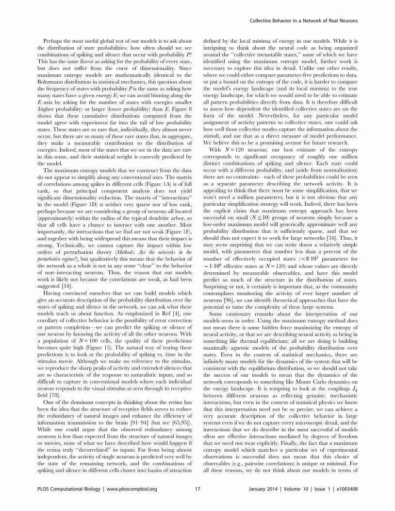
Perhaps the most useful global test of our models is to ask about

the distribution of state probabilities: how often should we see

combinations of spiking and silence that occur with probability P?

This has the same flavor as asking for the probability of every state,

but does not suffer from the curse of dimensionality. Since

maximum entropy models are mathematically identical to the

Boltzmann distribution in statistical mechanics, this question about

the frequency of states with probability P is the same as asking how

many states have a given energy E; we can avoid binning along the

E axis by asking for the number of states with energies smaller

(higher probability) or larger (lower probability) than E. Figure 8

shows that these cumulative distributions computed from the

model agree with experiment far into the tail of low probability

states. These states are so rare that, individually, they almost never

occur, but there are so many of these rare states that, in aggregate,

they make a measurable contribution to the distribution of

energies. Indeed, most of the states that we see in the data are rare

in this sense, and their statistical weight is correctly predicted by

the model.

The maximum entropy models that we construct from the data

do not appear to simplify along any conventional axes. The matrix

of correlations among spikes in different cells (Figure 1A) is of full

rank, so that principal component analysis does not yield

significant dimensionality reduction. The matrix of ‘‘interactions’’

in the model (Figure 1D) is neither very sparse nor of low rank,

perhaps because we are considering a group of neurons all located

(approximately) within the radius of the typical dendritic arbor, so

that all cells have a chance to interact with one another. Most

importantly, the interactions that we find are not weak (Figure 1F),

and together with being widespread this means that their impact is

strong. Technically, we cannot capture the impact within low

orders of perturbation theory (Methods: Are the networks in the

perturbative regime?), but qualitatively this means that the behavior of

the network as a whole is not in any sense ‘‘close’’ to the behavior

of non–interacting neurons. Thus, the reason that our models

work is likely not because the correlations are weak, as had been

suggested [34].

Having convinced ourselves that we can build models which

give an accurate description of the probability distribution over the

states of spiking and silence in the network, we can ask what these

models teach us about function. As emphasized in Ref [4], one

corollary of collective behavior is the possibility of error correction

or pattern completion—we can predict the spiking or silence of

one neuron by knowing the activity of all the other neurons. With

a population of N = 100 cells, the quality of these predictions

becomes quite high (Figure 15). The natural way of testing these

predictions is to look at the probability of spiking vs. time in the

stimulus movie. Although we make no reference to the stimulus,

we reproduce the sharp peaks of activity and extended silences that

are so characteristic of the response to naturalistic inputs, and so

difficult to capture in conventional models where each individual

neuron responds to the visual stimulus as seen through its receptive

field [78].

One of the dominant concepts in thinking about the retina has

been the idea that the structure of receptive fields serves to reduce

the redundancy of natural images and enhance the efficiency of

information transmission to the brain [91–94] (but see [65,95]).

While one could argue that the observed redundancy among

neurons is less than expected from the structure of natural images

or movies, none of what we have described here would happen if

the retina truly ‘‘decorrelated’’ its inputs. Far from being almost

independent, the activity of single neurons is predicted very well by

the state of the remaining network, and the combinations of

spiking and silence in different cells cluster into basins of attraction

defined by the local minima of energy in our models. While it is

intriguing to think about the neural code as being organized

around the ‘‘collective metastable states,’’ some of which we have

identified using the maximum entropy model, further work is

necessary to explore this idea in detail. Unlike our other results,

where we could either compare parameter-free predictions to data,

or put a bound on the entropy of the code, it is harder to compare

the model’s energy landscape (and its local minima) to the true

energy landscape, for which we would need to be able to estimate

all pattern probabilities directly from data. It is therefore difficult

to assess how dependent the identified collective states are on the

form of the model. Nevertheless, for any particular model

assignment of activity patterns to collective states, one could ask

how well those collective modes capture the information about the

stimuli, and use that as a direct measure of model performance.

We believe this to be a promising avenue for future research.

With N = 120 neurons, our best estimate of the entropy

corresponds to significant occupancy of roughly one million

distinct combinations of spiking and silence. Each state could

occur with a different probability, and (aside from normalization)

there are no constraints—each of these probabilities could be seen

as a separate parameter describing the network activity. It is

appealing to think that there must be some simplification, that we

won’t need a million parameters, but it is not obvious that any

particular simplification strategy will work. Indeed, there has been

the explicit claim that maximum entropy approach has been

successful on small (Nƒ10) groups of neurons simply because a

low-order maximum model will generically approximate well any

probability distribution that is sufficiently sparse, and that we

should thus not expect it to work for large networks [34]. Thus, it

may seem surprising that we can write down a relatively simple

model, with parameters that number less than a percent of the

number of effectively occupied states (v8:103 parameters for

*1:106 effective states at N = 120) and whose values are directly

determined by measurable observables, and have this model

predict so much of the structure in the distribution of states.

Surprising or not, it certainly is important that, as the community

contemplates monitoring the activity of ever larger number of

neurons [96], we can identify theoretical approaches that have the

potential to tame the complexity of these large systems.

Some cautionary remarks about the interpretation of our

models seem in order. Using the maximum entropy method does

not mean there is some hidden force maximizing the entropy of

neural activity, or that we are describing neural activity as being in

something like thermal equilibrium; all we are doing is building

maximally agnostic models of the probability distribution over

states. Even in the context of statistical mechanics, there are

infinitely many models for the dynamics of the system that will be

consistent with the equilibrium distribution, so we should not take

the success of our models to mean that the dynamics of the

network corresponds to something like Monte Carlo dynamics on

the energy landscape. It is tempting to look at the couplings Jij

between different neurons as reflecting genuine, mechanistic

interactions, but even in the context of statistical physics we know

that this interpretation need not be so precise: we can achieve a

very accurate description of the collective behavior in large

systems even if we do not capture every microscopic detail, and the

interactions that we do describe in the most successful of models

often are effective interactions mediated by degrees of freedom

that we need not treat explicitly. Finally, the fact that a maximum

entropy model which matches a particular set of experimental

observations is successful does not mean that this choice of

observables (e.g., pairwise correlations) is unique or minimal. For

all these reasons, we do not think about our models in terms of



their parameters, but rather as a description of the probability

distribution P(fsig) itself, which encodes the collective behavior of

the system.

The striking feature of the distribution over states is its extreme

inhomogeneity. The entropy of the distribution is not that much

smaller than it would be if the neurons made independent

decisions to spike or be silent, but the shape of the distribution is

very different; the network builds considerable structure into the

space of states, without sacrificing much capacity. The probability

of the same state repeating is many orders of magnitude larger

than expected for independent neurons, and this really is quite

startling (Figure 14). If we extrapolate to the full population of

,250 neurons in this correlated, interconnected patch of the

retina, the probability that two randomly chosen states of the

system are the same is roughly one percent. Thus, some

combination of spiking and silence across this huge population

should repeat exactly every few seconds. This is true despite the

fact that we are looking at the entire visual representation of a

small patch of the world, and the visual stimuli are fully

naturalistic. Although complete silence repeats more frequently,

a wide range of other states also recur, so that many different

combinations of spikes and silence occur often enough that we (or

the brain) can simply count them to estimate their probability.

This would be absolutely impossible in a population of nearly

independent neurons, and it has been suggested that these

repeated patterns provide an anchor for learning [12]. It is also

possible that the detailed structure of the distribution, including its

inhomogeneity, is matched to the statistical structure of visual

inputs in a way that goes beyond the idea of redundancy

reduction, occupying a regime in which strongly correlated activity

is an optimal code [17,18,49,97].

Building a precise model of activity patterns required us to

match the statistics of global activity (the probability that K out of

N neurons spike in the same small window of time). Several recent

works suggested alternative means of capturing the higher-order

correlations [12,98–103]. Particularly promising and computa-

tionally tractable amongst these models is the dichotomized

Gaussian (DG) model [100] that could explain correctly the

distribution of synchrony in the monkey cortex [104]. While DG

does well when compared with pairwise models on our data, it is

significantly less successful than the full K-pairwise models that we

have explored here. In particular, the DG predictions of three-

neuron correlations are much less accurate than in our model, and

the probability of coincidences is underestimated by an amount

that grows with increasing N (Figure S6). Elsewhere we have

explored a very simple model in which we ignore the identity of

the neurons and match only the global behavior [39]. This model

already has a lot of structure, including the extreme inhomoge-

neity that we have emphasized here. In the simpler model we can

exploit the equivalence between maximum entropy models and

statistical mechanics to argue that this inhomogeneity is equivalent

to the statement that the population of neurons is poised near a

critical surface in its parameter space, and we have seen hints of

this from analyses of smaller populations as well [6,9]. The idea

that biological networks might organize themselves to critical

points has a long history, and several different notions of criticality

have been suggested [31]. A sharp question, then, is whether the

full probability distributions that we have described here

correspond to a critical system in the sense of statistical physics,

and whether we can find more direct evidence for criticality in the

data, perhaps without the models as intermediaries.

Finally, we note that our approach to building models for the

activity of the retinal ganglion cell population is entirely

unsupervised: we are making use only of structure in the spike

trains themselves, with no reference to the visual stimulus. In this

sense, the structures that we discover here are structures that could

be discovered by the brain, which has no access to the visual

stimulus beyond that provided by these neurons. While there are

more structures that we could use—notably, the correlations

across time—we find it remarkable that so much is learnable from

just an afternoon’s worth of data. As it becomes more routine to

record the activity of such (nearly) complete sensory representa-

tions, it will be interesting to take the organism’s point of view [43]

more fully, and try to extract meaning from the spike trains in an

unsupervised fashion.

Methods

Ethics statementThis study was performed in strict accordance with the

recommendations in the Guide for the Care and Use of

Laboratory Animals of the National Institutes of Health. The

protocol was approved by the Institutional Animal Care and Use

Committee (IACUC) of Princeton University (Protocol 1827 for

guinea pigs and 1828 for salamanders).

ElectrophysiologyWe analyzed the recordings from the tiger salamander

(Ambystoma tigrinum) retinal ganglion cells responding to naturalistic

movie clips, as in the experiments of Refs. [4,36,65]. In brief,

animals were euthanized according to institutional animal care

standards. The retina was isolated from the eye under dim

illumination and transferred as quickly as possible into oxygenated

Ringer’s medium, in order to optimize the long-term stability

of recordings. Tissue was flattened and attached to a dialysis

membrane using polylysine. The retina was then lowered with

the ganglion cell side against a multi-electrode array. Arrays

were first fabricated in university cleanroom facilities [105].

Subsequently, production was contracted out to a commercial

MEMS foundry for higher volume production (Innovative Micro

Technologies, Santa Barbara, CA). Raw voltage traces were

digitized and stored for off-line analysis using a 252-channel

preamplifier (MultiChannel Systems, Germany). The recordings

were sorted using custom spike sorting software developed

specifically for the new dense array [36]. 234 neurons passed the

standard tests for the waveform stability and the lack of refractory

period violations. Of those, 160 cells whose firing rates were most

stable across stimulus repeats were selected for further analysis.

Within this group, the mean fraction of interspike intervals

(ISI) shorter than 2 ms (i.e., possible refractory violations) was

1:3:10{3.

Stimulus displayThe stimulus consisted of a short (t = 19 s) grayscale movie clip

of swimming fish and water plants in a fish tank, which was

repeated 297 times. The stimulus was presented using standard

optics, at a rate of 30 frames per second, and gamma corrected for

the display.

Data preparationWe randomly selected 30 subgroups of N~10,20, � � � ,120 cells

for analysis from the total of 160 sorted cells. In sum, we analyzed

30|12~360 groups of neurons, which we denote by SnN , where

N denotes the subgroup size, and n~1, � � � ,30 indexes the chosen

subgroup of that size. Time was discretized into Dt = 20 ms time

bins, as in our previous work [4,6,9]. The state of the retina was

represented by si(t)~z1({1) if the neuron i spiked at least once

(was silent) in a given time bin t. This binary description is



incomplete only in ,0.5% of the time bins that contain more than

one spike; we treat these bins as si~z1. Across the entire

experiment, the mean probability for a single neuron to make a

spike in a timebin (that is, si~z1) is ,3.1%. Time discretization

resulted in 953 time bins per stimulus repeat; 297 presented

repeats yielded a total of T~283,041 N-bit binary samples during

the course of the experiment for each subgroup.

Learning maximum entropy models from dataWe used a modified version of our previously published learning

procedure to compute the maximum entropy models given

measured constraints [37]; the proof of convergence for the core

of this L1-regularized maximum entropy algorithm is given in Ref.

[106]. Our new algorithm can use as constraints arbitrary

functions, not only single and pairwise marginals as before.

Parameters of the Hamiltonian are learned sequentially in an

order which greedily optimizes a bound on the log likelihood, and

we use a variant of histogram Monte Carlo to estimate the values

of constrained statistics during learning steps [107]. Monte Carlo

induces sampling errors on our estimates of these statistics, which

provide an implicit regularization for the parameters of the

Hamiltonian [106]. We verified the correctness of the algorithm

explicitly for groups of 10 and 20 neurons where exact numerical

solutions are feasible. We also verified that our MC sampling had

a long enough ‘‘burn-in’’ time to equilibrate, even for groups of

maximal size (N = 120), by starting the sampling repeatedly from

same vs different random initial conditions (100 runs each) and

comparing the constrained statistics, as well as the average and

variance of the energy and magnetization, across these runs; all

statistics were not significantly dependent on the initial state (two–

sample Kolmogorov-Smirnov test at significance level 0.05).

Supplementary Figure S1 provides a summary of the models we

have learned for populations of different sizes. In small networks

there is a systematic bias to the distribution of Jij parameters, but

as we look to larger networks this vanishes and the distribution of

Jij becomes symmetric. Importantly, the distribution remains quite

broad, with the standard deviation of Jij across all pairs declining

only slightly. In particular, the typical coupling does not decline as

*1=ffiffiffiffiffiNp

, as would be expected in conventional spin glass models

[70]. This implies, as emphasized previously [9], that the

‘‘thermodynamic limit’’ (very large N) for these systems will be

different from what we might expect based on traditional physics

examples.

We withheld a random selection of 20 stimulus repeats (test set)

for model validation, while training the model on the remaining

277 repeats. On training data, we computed the constrained

statistics (mean firing rates, covariances, and the K-spike

distribution), and used bootstrapping to estimate the error bars

on each of these quantities; the constraints were the only input to

the learning algorithm. Figure 1 shows an example reconstruction

for a pairwise model for N = 100 neurons; the precision of the

learning algorithm is shown in Figure 2.

The dataset consists of a total of T*300:103 binary pattern

samples, but he number of statistically independent samples must

be smaller: while the repeats are plausibly statistically independent,

the samples within each repeat are not. The variance for a binary

variable given its mean, hsii, is s2i,1~1{hsii2; with R indepen-

dent repeats, the error on the estimate in the average should

decrease as s2i,R~s2

i,1=R. By repeatedly estimating the statistical

errors with different subsets of repeats and comparing the expected

scaling of the error in the original data set with the data set where

we shuffle time bins randomly, thereby destroying the repeat

structure, we can estimate the effective number of independent

samples; we find this to be Tindep*110:103, about 37% of the total

number of samples, T.

We note that our largest models have v8:103 constrained

statistics that are estimated from at least 156 as many statistically

independent samples. Moreover, the vast majority of these

statistics are pairwise correlation coefficients that can be estimated

extremely tightly from the data, often with relative errors below

1%, so we do not expect overfitting on general grounds.

Nevertheless, we explicitly checked that there is no overfitting by

comparing the log likelihood of the data under the learned

maximum entropy model, for each of the 360 subgroups SnN , on

the training and testing set, as shown in Figure 3.

Parametrization of the K-pairwise modelThe parametrization of the K-pairwise Hamiltonian of Eq (20)

is degenerate, that is, there are multiple sets of coupling constants

fhi,Jij ,V (K)g that specify mathematically identical models. This

is because adjusting all local fields hi by a constant offset adds a

term linear in K to V (K); similarly, adjusting all pairwise

couplings Jij by a constant offset adds a quadratic term to V (K).

For comparing model predictions (i.e., observables, entropy, the

structure of the energy landscape etc) this is inconsequential, but

when model parameters are compared directly in Figure 5, one

must choose a gauge that will make the comparison of the

pairwise and K-pairwise parameters unbiased. Since there is no

V (K) in the pairwise model, we extract from the V (K) of the K-

pairwise model all those components that can be equivalently

parametrized by offsets to local fields and pairwise couplings. In

detail, we subtract best linear and quadratic fits from the

reconstructed V (K), such that the remaining V (K) only

constrains multi-point correlations that cannot be accounted for

by a choice of fields and pairwise interactions; the linear and

quadratic fit then give us adjustments to local fields and pairwise

interactions.

Exploring the energy landscapeTo find the metastable (MS) states, we start with a pattern fsig

that appears in the data, and attempt to flip spins i~1, � � � ,Nfrom their current state into {si, in order of increasing i. A flip

is retained if the energy of the new configuration is smaller than

before the flip. When none of the spins can be flipped, the

resulting pattern is recorded as the MS state. The set of MS

states found can depend on the manner in which descent is

performed, in particular when some of the states visited during

descent are on the ‘‘ridges’’ between multiple basins of attraction.

Note that whether a pattern is a MS state or not is independent

of the descent method; what depends on the method is which

MS states are found by starting from the data patterns. To

explore the structure of the energy landscape in Figure 11, we

started 1000 Metropolis MC simulations repeatedly in each of

the 10 most common MS states of the model; after each

attempted spin-flip, we checked whether the resulting state is still

in the basin of attraction of the starting MS state (by invoking the

descent method above), or whether it has crossed the energy

barrier into another basin. We histogrammed the transition

probabilities into other MS basins of attraction and, for

particular transitions, we tracked the transition paths to extract

the number of spin-flip attempts and the energy barriers. The

‘‘basin size’’ of a given MS state is the number of patterns in the

recorded data from which the given MS state is reached by

descending on the energy landscape. The results presented in

Figure 11 are typical of the transitions we observe across multiple

subnetworks of 120 neurons.



Computing the entropy and partition function of themaximum entropy distributions

Entropy estimation is a challenging problem. As explained in

the text, the usual approach of counting samples and identifying

frequencies with probabilities will fail catastrophically in all the

cases of interest here, even if we are free to draw samples from our

model rather than from real data. Within the framework of

maximum entropy models, however, the equivalence to statistical

mechanics gives us several tools. Here we summarize the evidence

that these multiple tools lead to consistent answers, so that we can

be confident in our estimates.

Our first try at entropy estimation is based on the heat capacity

integration in Eq. (29). To begin, with N~10,20 neurons, we can

enumerate all 2N states of the network and hence we can find the

maximum entropy distributions exactly (with no Monte Carlo

sampling). From these distributions we can also compute the

entropy exactly, and it agrees with the results of the heat capacity

integration. Indeed, there is good agreement for the entire

distribution, with Jensen-Shannon divergence between exact

maximum entropy solutions and solutions using our reconstruction

procedure at ,1026. As a second check, now usable for all N, we

note that the entropy is zero at T = 0, but S~N bits at T~?.

Thus we can do the heat capacity integration from T = 1 to T~?instead of T = 0 to T = 1, and we get essentially the same result for

the entropy (mean relative difference of 8:8:10{3 across 30

networks at N = 100 and N = 120).

Leaning further on the mapping to statistical physics, we realize

that the heat capacity is a summary statistic for the density of

states. There are Monte Carlo sampling methods, due to Wang

and Landau [73] (WL), that aim specifically at estimating

this density, and those allow us to compute the entropy from a

single simulation run. Based on the benchmarks of the WL method

that we performed (convergence of the result with histogram

refinement) we believe that the entropy estimate from the WL MC

has a fractional bias that is at or below 2:10{3. The results, in

Figure S2A, are in excellent agreement with the heat capacity

integration.

K-pairwise models have the attractive feature that, by

construction, they match exactly the probability of the all-silent

pattern, P(K~0), seen in the data. As explained in the main text,

this means that we can ‘‘measure’’ the partition function, Z, of our

model directly from the probability of silence. Then we can

compute the average energy hEi from a single MC sampling run,

and find the entropy for each network. As shown in Figures S2B

and C, the results agree both with the heat capacity integration

and with the Wang–Landau method, to an accuracy of better than

1%.

The error on entropy estimation from the probability of

silence has two contributions: the first has to do with the error in

P(0) that contributes to error in Z by Eq (30), and the second

with the estimate of the mean energy, hEi, of the model. By

construction of the model, P(0) needs to be matched to data, but

in fact that match is limited by the error bar on P(0) itself

estimated from data, and on how well the model reproduces this

observable; these two errors combine to give a fractional error of

a few tenths of a percent. From this error one may then compute

the fractional error in Z; for N = 120 groups of neurons, this is

on average *3:10{3. For the entropy estimation, we also need

the average energy; this itself can be estimated through a long

Metropolis MC sampling. The sampling is unbiased, but with an

error of typically between half and a percent, for N = 120 sets.

Together, these errors combine into a conservative error

estimate of ,1% for the entropy computed from the silence

and from the average energy, although the true error might in

fact be smaller.

Finally, there are methods that allow us to estimate entropy by

counting samples even in cases where the number of samples is

much smaller than the number of states [71] (NSB). The NSB

method is not guaranteed to work in all cases, but the comparison

with the entropy estimates from heat capacity integration (Figure

S3A) suggests that so long as N,50, NSB estimates are reliable

(see also [108]). Supplementary Figure S3B shows that the NSB

estimate of the entropy does not depend on the sample size for

N,50; if we draw from our models a number of samples equal to

the number found in the data, and then ten times more, we see

that the estimated entropy changes by just a few percent, within

the error bars. This is another signature of the accuracy of the

NSB estimator for N,50. As N increases, these direct estimates of

entropy become significantly dependent on the sample size,

and start to disagree with the heat capacity integration. The

magnitude of these systematic errors depends on the structure

of the underlying distribution, and it is thus interesting that

NSB estimates of the entropy from our model and from the real

data agree with one another up to N = 120, as shown in Figure

S3C.

Are real networks in the perturbative regime?The pairwise correlations between neurons in this system are

quite weak. Thus, if we make a model for the activity of just two

neurons, treating them as independent is a very good approx-

imation. It might seem that this statement is invariant to the

number of neurons that we consider—either correlations are

weak, or they are strong. But this misses the fact that weak but

widespread correlations can have a non–perturbative effect on

the structure of the probability distribution. Nonetheless, it has

been suggested that maximum entropy methods are successful

only because correlations are weak, and hence that we can’t

really capture non–trivial collective behaviors with this approach

[34].

While independent models fail to explain the behavior of even

small groups of neurons [4], it is possible that groups of neurons

might be in a weak perturbative regime, where the contribution of

pairwise interactions could be treated as a small perturbation to

the independent Hamiltonian, if the expansion was carried out in

the correct representation [34]. Of course, with finite N, all

quantities must be analytic functions of the coupling constants, and

so we expect that, if carried to sufficiently high order, any

perturbative scheme will converge—although this convergence

may become much slower at larger N, signaling genuinely

collective behavior in large networks.

To make the question of whether correlations are weak or

strong precise, we ask whether we can approximate the

maximum entropy distribution with the leading orders of

perturbation theory. There are a number of reasons to think

that this won’t work [109–112], but in light of the suggestion

from Ref [34] we wanted to explore this explicitly. If correlations

are weak, there is a simple relationship between the correlations

Cij and the corresponding interactions Jij [34,113]. We see in

Figure S4A that this relationship is violated, and the conse-

quence is that models built by assuming this perturbative

relationship are easily distinguishable from the data even at

N = 15 (Figure S4B). We conclude that treating correlations as a

small perturbation is inconsistent with the data. Indeed, if we try

to compute the entropy itself, it can be shown that even going

out to fourth order in perturbation theory is not enough once

N.10 [111,112].



Supporting Information

Figure S1 Interactions in the (K-)pairwise model. (A)

The distributions of pairwise couplings, Jij, in pairwise models of

Eq (19), for different network sizes (N). The distribution is pooled

over 30 networks at each N. (B) The mean (solid) and s.d. (dashed)

of the distributions in (A) as a function of network size (black); the

mean and s.d. of the corresponding distributions for K-pairwise

models as a function of network size (red).

(PDF)

Figure S2 Precision of entropy estimates. (A) Entropy

estimation using heat capacity integration (x-axis) from Eq (29)

versus entropy estimation using the Wang-Landau sampling

method (y-axis) [73]. Each plot symbol is one subnetwork of

either N = 100 or N = 120 neurons (circles = pairwise models,

crosses = K-pairwise models). The two sampling methods yield

results that agree to within ,1%. (B) Fractional difference

between the heat capacity method and the entropy determined

from the

all-silent pattern. The histogram is over 30 networks at N = 100

and 30 at N = 120, for the K-pairwise model. (C) Fractional

difference between the Wang-Landau sampling method and the

entropy determined from the all-silent pattern. Same convention

as in (B).

(PDF)

Figure S3 Sample-based entropy estimation. (A) The bias

in entropy estimates computed directly from samples drawn from

K-pairwise models. The NSB entropy estimate [71] in bits per

neuron computed using *3:105 samples from the model (same

size as the experimental data set) on y-axis; the true entropy (using

heat capacity integration) method on x-axis. Each dot represents

one subnetwork of a particular size (N, different colors). For small

networks (Nƒ40) the bias is negligible, but estimation from

samples significantly underestimates the entropy for larger

networks. (B) The fractional bias of the estimator as a function

of N (black dots = data from (A), gray dots = using 10 fold more

samples). Red line shows the mean 6 s.d. over 30 subnetworks at

each size. (C) The NSB estimation of entropy from samples drawn

from the model (x-axis) vs the samples from real experiment (y-

axis); each dot is a subnetwork of a given size (color as in (A)). The

data entropy estimate is slightly smaller than that of the model, as

is expected for true entropy; for estimates from finite data this

would only be expected if the biases on data vs MC samples were

the same.

(PDF)

Figure S4 Perturbative vs exact solution for the pair-wise maximum entropy models. (A) The comparison of

couplings Jij for a group of N~5,10,15,20 neurons, computed

using the exact maximum entropy reconstruction algorithm, with

the lowest order perturbation theory result, Jij~14

log cij, where

cij~h~ssi~ssji=(h~ssiih~ssji) and ~ssi~0:5(1zsi) [34,113]. In the case of

larger networks, the perturbative Jij deviate more and more from

equality (black line). Inset: the average absolute difference between

the true and perturbative coupling, normalized by the average true

coupling. (B) The exact pairwise model, Eq (19), can be compared

to the distribution Pexpt( sif g), sampled from data; the olive line

(circles) shows the Jensen-Shannon divergence (corrected for finite

sample size) between the two distributions, for four example

networks of size N~5,10,15,20. The turquoise line (squares)

shows the same comparison in which the pairwise model

parameters, g~ hi,Jij

� �, were calculated perturbatively. The black

line shows the DJS between two halves of the data for the four

selected networks.

(PDF)

Figure S5 Predicted vs real distributions of energy, E,for the pairwise model. The cumulative distribution of

energies, Cv(E) from Eq (22), for the patterns generated by the

pairwise models (red) and the data (black), in a population of 120

neurons. Inset shows the high energy tails of the distribution,

Cw(E) from Eq (24); dashed line denotes the energy that

corresponds to the probability of seeing the pattern once in an

experiment. This figure is analogous to Figure 8; the same group

of neurons is used here.

(PDF)

Figure S6 Dichotomized Gaussian model performancefor a group of N = 120 neurons. (A) The distribution of

synchronous spikes, P(K), in the data (black) and in the DG model

fit to data (red). For this network, DG predicts P(0)~0:158; the

true value is P(0)~0:248. (B) The comparison of three-point

correlations estimated from data (x-axis) and predicted by the two

models (y-axis; red = DG, black = K-pairwise). As in Figure 7,

three-point correlations are binned; shown are the means for the

predictions in a given bin, error-bars are omitted for clarity. DG

underperforms the K-pairwise model specifically for negative

correlations. (C) The probability of coincidences, analogous to

Figure 14, computed for the DG model (red) and compared to

data (black); gray line is the independent model.

(PDF)

Figure S7 Maximum entropy models for the checker-board stimulation. We stimulated a separate retina with a

checkerboard stimulus. The square check size was 69 mm, smaller

than the typical size of the ganglion cell receptive fields. Each

check was randomly selected to be either black or white on each

frame displayed at a rate of 30 Hz. The entire stimulus consisted

of 69 repeats of 30 seconds each, and subgroups of up to 120

neurons were analyzed. (A) Distribution of synchrony, P(K), for a

group of 120 neurons, in the data (red), as predicted by the

pairwise model (black), and by the independent model (gray). (B)

As the network of N neurons gets larger, the discrepancy in the

prediction of the probability of silence, P(0), grows in a

qualitatively similar way as under naturalistic stimulation. (C) K-

pairwise models capture the distribution of energies very well even

at N = 120 (cf. Figure 8 for an analogous plot for natural

stimulation). (D) Under checkerboard stimulation, the distribution

of codewords is less correlated than under the natural stimulation,

as quantified by the ratio of the entropy to the independent

entropy, shown as a function of subgroup size N.

(PDF)

Acknowledgments

We thank A Cavagna, I Giardina, T Mora, SE Palmer, GJ Stephens, and

A Walczak for many helpful discussions.

Author Contributions

Conceived and designed the experiments: GT OM DA ES WB MJB.

Performed the experiments: OM DA MJB. Analyzed the data: GT OM

DA WB MJB. Wrote the paper: GT OM WB MJB.



References

1. Hopfield JJ (1982) Neural networks and physical systems with emergent

collective computational abilities. Proc Natl Acad Sci (USA) 79: 2554–8.

2. Amit DJ (1989) Modeling Brain Function: The World of Attractor Neural

Networks. Cambridge: Cambridge University Press.

3. Hertz J, Krogh A & Palmer RG (1991) Introduction to the Theory of Neural

Computation. Redwood City: Addison Wesley.

4. Schneidman E, Berry MJ II, Segev R & Bialek W (2006) Weak pairwisecorrelations imply strongly correlated network states in a neural population.

Nature 440: 1007–1012.

5. Shlens J, Field GD, Gaulthier JL, Grivich MI, Petrusca D, Sher A, Litke AM &

Chichilnisky EJ (2006) The structure of multi-neuron firing patterns in primateretina. J Neurosci 26: 8254–8266.

6. Tkacik G, Schneidman E, Berry MJ II & Bialek W (2006) Ising models fornetworks of real neurons. arXiv.org: q-bio/0611072.

7. Yu S, Huang D, Singer W & Nikolic D (2008) A small world of neuronalsynchrony. Cereb Cortex 18: 2891–2901.

8. Tang A, Jackson D, Hobbs J, Chen W, Smith JL, Patel H, Prieto A, PetruscamD Grivich MI, Sher A, Hottowy P, Dabrowski W, Litke AM & Beggs JM (2008)

A maximum entropy model applied to spatial and temporal correlations from

cortical networks in vitro. J Neurosci 28: 505–518.

9. Tkacik G, Schneidman E, Berry MJ II & Bialek W (2009) Spin–glass models for

a network of real neurons. arXiv.org: 0912.5409.

10. Shlens J, Field GD, Gaulthier JL, Greschner M, Sher A, Litke AM &

Chichilnisky EJ (2009) The structure of large–scale synchronized firing inprimate retina. J Neurosci 29: 5022–5031.

11. Ohiorhenuan IE, Mechler F, Purpura KP, Schmid AM, Hu Q & Victor JD(2010) Sparse coding and higher–order correlations in fine–scale cortical

networks. Nature 466: 617–621.

12. Ganmor E, Segev R & Schniedman E (2011) Sparse low–order interaction

network underlies a highly correlated and learnable neural population code.Proc Natl Acad Sci (USA) 108: 9679–9684.

13. Vasquez JC, Marre O, Palacios AG, Berry MJ II & Cessac B (2012) Gibbsdistribution analysis of temporal correlations structure in retina ganglion cells.

J Physiol Paris 3–4: 120–127.

14. Granot-Atedgi E, Tkacik G, Segev R & Schneidman E (2013) Stimulus-

dependent maximum entropy models of neural population codes. PLoS

Comput Biol 9: e1002922.

15. Ganmor E, Segev R & Schneidman E (2011) The architecture of functional

interaction networks in the retina. J Neurosci 31: 3044–3054.

16. Tkacik G, Prentice JS, Victor JD & Balasubramanian V (2010) Local statistics

in natural scenes predict the saliency of synthetic textures. Proc Natl Acad Sci(USA) 107: 18149–18154.

17. Stephens GJ, Mora T, Tkacik G & Bialek W (2013) Statistical thermodynamicsof natural images. Phys Rev Lett 110: 018701.

18. Saremi S & Sejnowski TJ (2013) Hierarchical model of natural images and theorigin of scale invariance. Proc Natl Acad Sci (USA) 110: 3071–3076.

19. Lezon TR, Banavar JR, Cieplak M, Maritan A & Federoff NV (2006) Usingthe principle of entropy maximization to infer genetic interaction networks

from gene expression patterns. Proc Natl Acad Sci (USA) 103: 19033–19038.

20. Tkacik G (2007) Information Flow in Biological Networks. Dissertation,

Princeton University.

21. Bialek W & Ranganathan R (2007) Rediscovering the power of pairwise

interactions. arXiv.org: 0712.4397.

22. Seno F, Trovato A, Banavar JR & Maritan A (2008) Maximum entropy

approach for deducing amino acid interactions in proteins. Phys Rev Lett 100:078102.

23. Weigt M, White RA, Szurmant H, Hoch JA & Hwa T (2009) Identification ofdirect residue contacts in protein–protein interaction by message passing. Proc

Natl Acad Sci (USA) 106: 67–72.

24. Halabi N, Rivoire O, Leibler S & Ranganathan R (2009) Protein sectors:Evolutionary units of three–dimensional structure. Cell 138: 774–786.

25. Mora T, Walczak AM, Bialek W & Callan CG Jr (2010) Maximum entropymodels for antibody diversity. Proc Natl Acad Sci (USA) 107: 5405–5410.

26. Marks DS, Colwell LJ, Sheridan R, Hopf TA, Pagnani A, Zecchina R &Sander C (2011) Protein 3D structure computed from evolutionary sequence

variation. PLoS One 6: e28766.

27. Sulkowska JI, Morocos F, Weigt M, Hwa T & Onuchic JN (2012) Genomics–

aided structure prediction. Proc Natl Acad Sci (USA) 109: 10340–10345.

28. Stephens GJ & Bialek W (2010) Statistical mechanics of letters in words. Phys

Rev E 81: 066119.

29. Bialek W, Cavagna A, Giardina I, Mora T, Silvestri E, Viale M & Walczak A

(2012) Statistical mechanics for natural flocks of birds. Proc Natl Acad Sci(USA) 109: 4786–4791.

30. Shemesh Y, Sztainberg Y, Forkosh O, Shlapobersky T, Chen A & SchneidmanE (2013) High-order social interactions in groups of mice. Elife 2: e00759.

31. Mora T & Bialek W (2010) Are biological systems poised at criticality? J StatPhys 144: 268–302.

32. Nirenberg S & Victor J (2007) Analyzing the activity of large populations ofneurons: How tractable is the problem. Curr Opin Neurobiol 17: 397–400.

33. Roudi Y, Aurell E & Hertz JA (2009) Statistical physics of pairwise probability

models. Front Comput Neurosci 3: 22.

34. Roudi Y, Nirenberg S & Latham PE (2009) Pairwise maximum entropy modelsfor studying large biological systems: when they can work and when they can’t.

PLoS Comput Biol 5: e1000380.

35. Roudi Y, Trycha J & Hertz J (2009) The Ising model for neural data: modelquality and approximate methods for extracting functional connectivity. Phys

Rev E 79: 051915.

36. Marre O, Amodei D, Deshmukh N, Sadeghi K, Soo F, Holy TE, & Berry MJII (2012) Mapping a complete neural population in the retina. J Neurosci 32:

14859–14873.

37. Broderick T, Dudik M, Tkacik, G Schapire RE & Bialek W (2007) Fastersolutions of the inverse pairwise Ising problem. arXiv.org: 0712.2437.

38. Treves A, Panzeri S, Rolls ET, Booth M & Wakeman EA (1999) Firing rate

distributions and efficiency of information transmission in inferior temporalcortex neurons to natural visual stimuli. Neural Comput 11: 601–631.

39. Tkacik G, Marre O, Mora T, Amodei D, Berry MJ II & Bialek W (2013) The

simplest maximum entropy model for collective behavior in a neural network.J Stat Mech P03011.

40. Okun M, Yger P, Marguet SL, Gerard-Mercier F, Benucci A, Katzner S, Busse

L, Carandini M & Harris KD (2012) Population rate dynamics and multi

neuron firing patterns in sensory cortex. J Neurosci 32: 17108–17119.

41. Jaynes ET (1957) Information theory and statistical mechanics. Phys Rev 106:

620–630.

42. Cessac B & Cofre R (2013) Spike train statistics and Gibbs distributions.J Physiol Paris pii: S0928-4257. arXiv.org:1302.5007.

43. Rieke F, Warland D, de Ruyter van Steveninck RR & Bialek W (1997) Spikes:

Exploring the Neural Code. Cambridge: MIT Press.

44. Bazaraa MS, Sherali HD & Shetty CM (2005) Nonlinear programming:Theory and algorithms. Hoboken NJ, , USA: Wiley & Sons.

45. Pillow JW, Shlens J, Paninski L, Sher A, Litke AM, Chichilnisky EJ &

Simoncelli EP (2008) Spatio-temporal correlations and visual signalling in acomplete neuronal population. Nature 454: 995–999.

46. Fairhall AL, Burlingame CA, Narasimhan R, Harris RA, Puchalla JL & Berry

MJ II (2006) Selectivity for multiple stimulus features in retinal ganglion cells.

J Neurophysiol 96: 2724–2738.

47. Keat J, Reinagel P, Reid RC & Meister M(2001) Predicting every spike: a

model for the responses of visual neurons. Neuron 30: 803–817.

48. Sadeghi KS (2009) Progress on Deciphering the Retinal Code. Dissertation,Princeton University.

49. Tkacik G, Prentice JS, Balasubramanian V & Schneidman E (2010) Optimal

population coding by noisy spiking neurons. Proc Natl Acad Sci (USA) 107:

14419–14424.

50. Tkacik G, Granot-Atedgi E, Segev R & Schneidman E (2013) Retinal metric: a

stimulus distance measure derived from population neural responses. Phys Rev

Lett 110: 058104.

51. Ganmor E (2013) Noise, structure and adaptation in neural population codes.

Thesis. Weizmann Institute of Science.

52. Perkel D & Bullock T (1968) Neural coding. Neurosci Res Program Bull 6:

221–343.

53. Ginzburg I & Sompolinsky H (1994) Theory of correlations in stochastic neural

networks. Phys Rev E 50: 3171–3191.

54. Hopfield JJ (2008) Searching for memories, sudoku, implicit check bits, and theiterative use of not–always–correct rapid neural computation. Neural Comp

20: 1119–1164.

55. Field D (1987) Relations between the statistics of natural images and the

response properties of cortical cells. J Opt Soc A 4: 2379–2394.

56. Dong DW & Atick JJ (1995) Statistics of natural time-varying images. Network

6: 345–358.

57. Ruderman DL & Bialek W (1994) Statistics of natural images: scaling in thewoods. Phys Rev Lett 73: 814–817.

58. Schwartz O & Simoncelli EP (2001) Natural signal statistics and sensory gain

control. Nat Neurosci 4: 819–825 (2001).

59. Bethge M & Berens P (2008) Near-maximum entropy models for binary neuralrepresentations of natural images. In: Platt J et al eds. Adv Neural Info Proc Sys

20: 97–104. Cambridge, MA: MIT Press.

60. Stephens GJ, Mora T, Tkacik G & Bialek W (2013) Statistical thermodynamicsof natural images. Phys Rev Lett 110: 018701.

61. Mastronarde DN (1983) Interactions between ganglion cells in cat retina.

J Neurophysiol 49: 350–365.

62. DeVries SH (1999) Correlated firing in rabbit retinal ganglion cells.J Neurophysiol 81: 908–920.

63. Brivanlou IH, Warland DK & Meister M (1998) Mechanisms of concerted

firing among retinal ganglion cells. Neuron 20: 527–539.

64. Trong PK & Rieke F (2008) Origin of correlated activity between parasolretinal ganglion cells. Nat Neurosci 11: 1343–1351.

65. Puchalla JL, Schneidman E, Harris RA & Berry MJ II (2005) Redundancy in

the population code of the retina. Neuron 46: 493–504.

66. Segev R, Puchalla J & Berry MJ II (2006) Functional organization of retinalganglion cells in the salamander retina. J Neurophysiol 95: 2277–2292.



67. Schneidman E, Still S, Berry MJ II & Bialek W (2003) Network information

and connected correlations. Phys Rev Lett 91: 238701.

68. Hopfield JJ & Tank DW (1985) ‘‘Neural’’ computation of decisions inoptimization problems. Biol Cybern 52: 141–152.

69. Hopfield JJ & Tank DW (1986) Computing with neural circuits: a model.Science 233: 625–633.

70. Mezard M, Parisi G & Virasoro MA (1987) Spin Glass Theory and Beyond.

Singapore: World Scientific

71. Nemenman I, Shafee F & Bialek W (2001) Entropy and inference, revisited.

Adv Neural Info Proc Syst 14: 471–478.

72. Landau DP & Binder K (2000) Monte Carlo Simulations in Statistical Physics.Cambridge, UK: Cambridge University Press.

73. Wang F & Landau DP (2001) Efficient, multiple-range random walk algorithm

to calculate the density of states. Phys Rev Lett 86: 2050–2053.

74. Cover TM & Thomas JA (1991) Elements of Information Theory. New York:

Wiley.

75. Lanford OE III (1973) Entropy and equilibrium states in classical statistical

mechanics. Statistical Mechanics and Mathematical Problems, Lenard A ed.,

pp. 1–113. Berlin: Springer Verlag.

76. Landau LD and Lifshitz EM (1977) Statistical Physics. Oxford: Pergamon.

77. Berry MJ II, Warland DK & Meister M (1997) The structure and precision of

retinal spike train. Proc Natl Acad Sci (USA) 94: 5411–5416.

78. van Hateren JH, Ruttiger L, Sun H & Lee BB (2002) Processing of natural

temporal stimuli by macaque retinal ganglion cells. J Neurosci 22: 9945–9960.

79. Shapley RM & Victor JD (1978) The effect of contrast on the transferproperties of cat retinal ganglion cells. J Physiol 285: 275–298.

80. Victor JD & Shapley RM (1979) Receptive field mechanisms of cat X and Yretinal ganglion cells. J Gen Physiol 74: 275–298.

81. Mante V, Bonin V & Carandini M (2008) Functional mechanisms shaping

lateral geniculate responses to artificial and natural stimuli. Neuron 58: 625–638.

82. Chen EY, Marre O, Fisher C, Schwartz G, Levy J, da Silveira RA & Berry MJ

II (2013) Alert response to motion onset in the retina. J Neurosci 33: 120–132.

83. Dan Y, Atick JJ & Reid RC (1996) Efficient coding of natural scenes in lateral

geniculate nucleus: experimental test of a computational theory. J Neurosci 16:3351–3362.

84. Theunissen FE, Sen K, and Doupe AJ (2000) Spectral-temporal receptive fields

of nonlinear auditory neurons obtained using natural sounds. J Neurosci 20:2135–2331.

85. Stopfer M, Jayaraman V & Laurent G (2003) Intensity versus identity coding in

an olfactory system. Neuron 39: 991–1004.

86. Machens CK, Romo R & Brody CD (2010) Functional, but not anatomical,

separation of ‘‘what’’ and ‘‘when’’ in prefrontal cortex. J Neurosci 30: 350–360.

87. Churchland MM, Cunningham JP, Kaufman MT, Ryu SI & Shenoy KV(2010) Cortical preparatory activity: representation of movement or first cog in

a dynamical machine? Neuron 68: 387–400.

88. Rutishauser U, Kotowicz A & Laurent G (2013) A method for closed-loop

presentation of sensory stimuli conditional on the internal brain-state of awake

animals. J Neurosci Methods 215: 139–155.

89. Segev R, Goodhouse J, Puchalla JL & Berry MJ II (2004) Recording spikes

from a large fraction of the ganglion cells in a retinal patch. Nat Neurosci 7:

1155–1162.

90. Marre O, Boustani SE, Fregnac Y & Destexhe A (2009) Prediction of spatio–

temporal patterns of neural activity from pairwise correlations. Phys Rev Lett102: 138101.

91. Barlow HB (1961) Possible principles underlying the transformation of sensory

messages. In: Rosenblith W, ed. Sensory communication, pp 217–234.Cambridge, USA: MIT Press.

92. Attneave F (1954) Some informational aspects of visual perception. Psychol Rev

61: 183–193.93. Atick JJ & Redlich AN (1990) Towards a theory of early visual processing.

Neural Comput 2: 308–320.94. van Hdateren JH (1992) Real and optimal neural images in early vision. Nature

360: 68–70.

95. Barlow H (2001) Redundancy reduction revisited. Network 12: 241–253.96. Alivisatos AP, Chun M, Church GM, Greenspan RJ, Roukes ML & Yuste R,

(2012) The brain activity map project and the challenge of functionalconnectomics. Neuron 74, 970–974.

97. Sourlas N (1989) Spin-glass models as error-correcting codes. Nature 339: 693–695.

98. Bohte SM, Spekreijse & Roelfsema PR (2000) The effects of pairwise and

higher-order correlations in the firing rate of a postsynaptic neuron. NeuralComput 12: 153–179.

99. Amari S-I, Nakahara H, Wu S & Sakai Y (2003) Synchronous firing andhigher-order interactions in neuron pool. Neural Comput 15: 127–142.

100. Macke JH, Opper M & Bethge M (2011) Common input explains higher-order

correlations and entropy in a simple model of neural population activity. PhysRev Lett 106: 1–4.

101. Santos GS, Gireesh ED, Plenz D & Nakahara H (2010) Hierarchicalinteraction structure of neural activities in cortical slice cultures. J Neurosci

30: 8720–8733.102. Shimazaki H, Sadeghi K, Ikegaya Y & Toyoizumi T (2012) The simultaneous

silence of neurons explains higher-order interactions in ensemble spiking

activity. Cosyne 2013, Salt Lake City, USA.103. Koster U, Sohl-Dickstein J, Gray CM & Olshausen BA (2013) Higher order

correlations within cortical layers dominate functional connectivity inmicrocolumns. arXiv.org:1301.0050.

104. Yu S, Yang H, Nakahara H, Santos GS, Nikolic D & Plenz D (2011) Higher-

order interactions characterized in cortical activity. J Neurosci 31: 17514–17526.

105. Amodei D, Schwartz G & Berry MJ II (2008) Correlations and the structure ofthe population code in a dense patch of the retina. In: Stett A ed. Proceedings

MEA Meeting. BIOPRO Baden-Wurttemberg, 2008. pp. 197.106. Dudik M, Phillips SJ & Schapire RE (2004) Performance guarantees for

regularized maximum entropy density estimation. Proceedings 17th Annual

conference on learning theory.107. Ferrenberg AM & Swendsen RH (1988) New Monte Carlo technique for

studying phase transitions. Phys Rev Lett 61: 2635–2638.108. Berry MJ II, Tkacik G, Dubuis J, Marre O, Azerado da Silveira R (2013) A

simple method for estimating the entropy of neural activity. J Stat Mech

P03015.109. Cocco S, Leibler S & Monasson R (2009) Neuronal couplings between retinal

ganglion cells inferred by efficient inverse statistical physics methods. Proc NatlAcad Sci (USA) 106: 14058–14062.

110. Cocco S & Monasson R (2011) Adaptive cluster expansion for inferringBoltzmann machines with noisy data. Phys Rev Lett 106: 090601.

111. Azhar F (2008) An Information Theoretic Study of Neural Populations.

Dissertation. University of California at Santa Barbara.112. Azhar F & Bialek W (2010) When are correlations strong? arXiv.org: 1012.5987.

113. Sessak V & Monasson R (2009) Small-correlation expansions for the inverseIsing problem. J Phys A 42: 055001.



Searching for Collective Behavior in a Large Network of Sensory...

Documents

Transcript of Searching for Collective Behavior in a Large Network of Sensory...