Search Algorithms

and Tables

Chapter 11

Tables

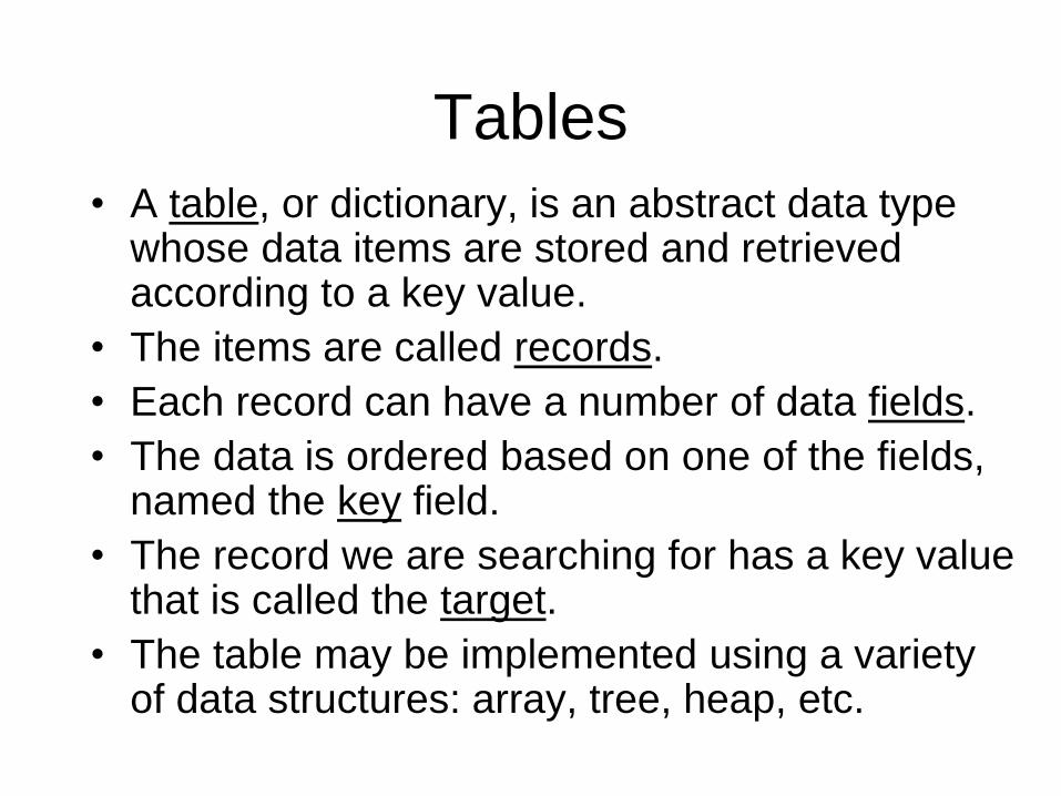
• A table, or dictionary, is an abstract data type whose data items are stored and retrieved according to a key value.

• The items are called records.

• Each record can have a number of data fields.

• The data is ordered based on one of the fields, named the key field.

• The record we are searching for has a key value that is called the target.

• The table may be implemented using a variety of data structures: array, tree, heap, etc.

Sequential Searchpublic static int search(int[] a,

int target) {

int i = 0;

boolean found = false;

while ((i < a.length) && ! found) {

if (a[i] == target)

found = true;

else i++;

}

if (found) return i;

else return –1;

}

Sequential Search on Tablespublic static int search(someClass[] a,

int target) {

int i = 0;

boolean found = false;

while ((i < a.length) && !found){

if (a[i].getKey() == target)

found = true;

else i++;

}

if (found) return i;

else return –1;

}

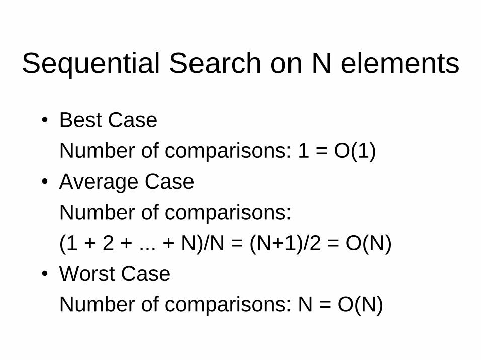
Sequential Search on N elements

• Best Case

Number of comparisons: 1 = O(1)

• Average Case

Number of comparisons:

(1 + 2 + ... + N)/N = (N+1)/2 = O(N)

• Worst Case

Number of comparisons: N = O(N)

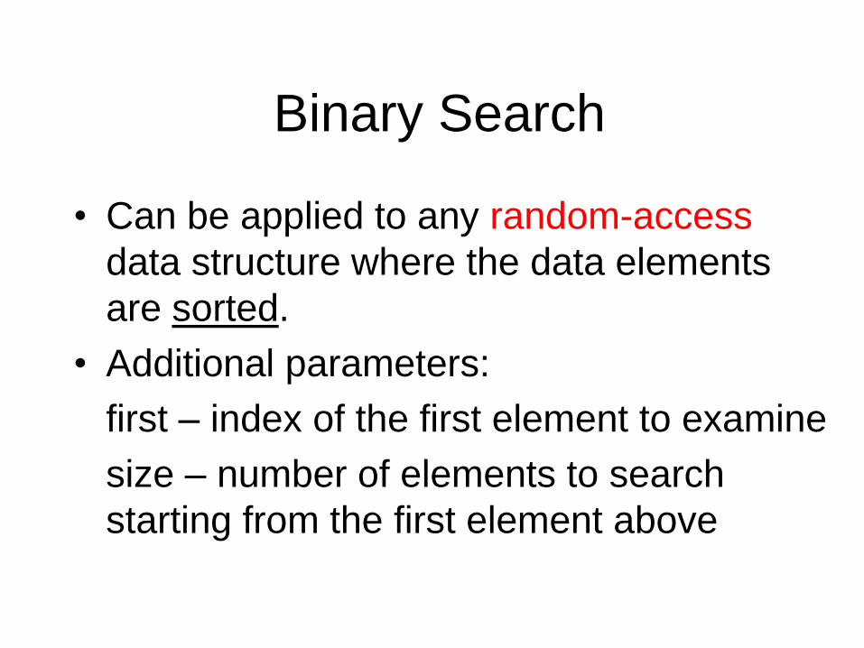
Binary Search

• Can be applied to any random-access

data structure where the data elements

are sorted.

• Additional parameters:

first – index of the first element to examine

size – number of elements to search

starting from the first element above

Binary Search

• Precondition:

If size > 0, then the data structure must have size elements starting with the element denoted as the first element. In addition, these elements are sorted.

• Postcondition:

If target appears, the position of the target is returned (a non-negative integer). Otherwise, -1 is returned.

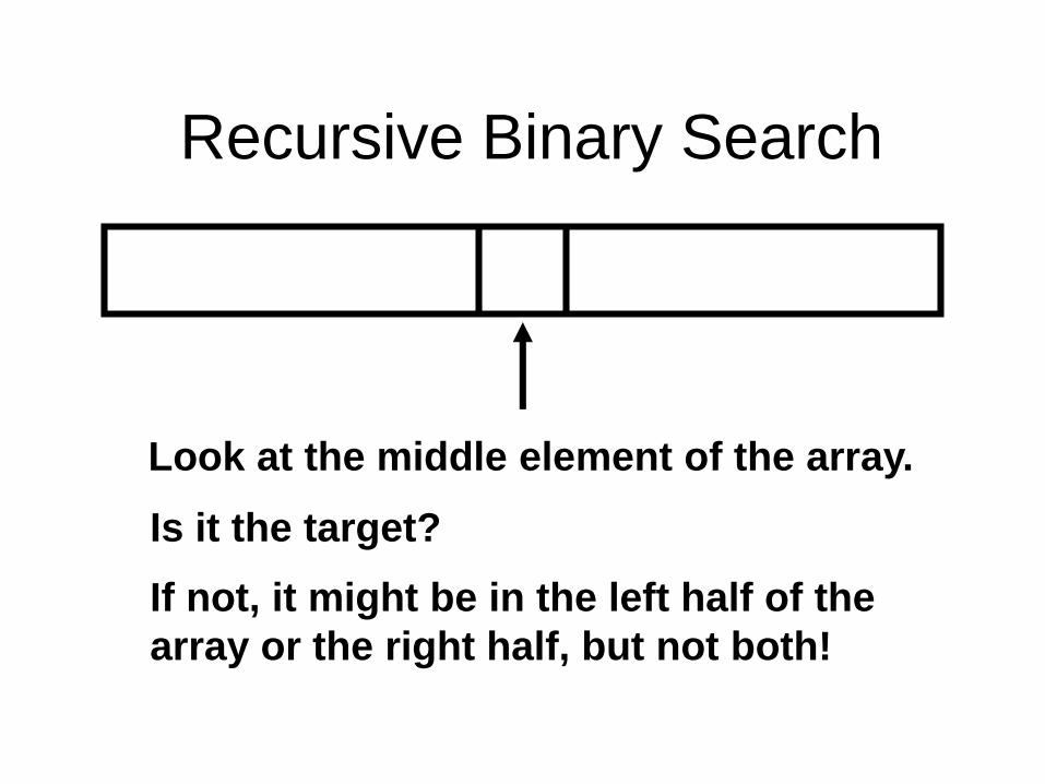
Recursive Binary Search

Look at the middle element of the array.

Is it the target?

If not, it might be in the left half of the

array or the right half, but not both!

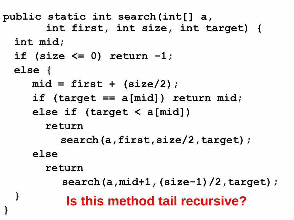
public static int search(int[] a,

int first, int size, int target) {

int mid;

if (size <= 0) return –1;

else {

mid = first + (size/2);

if (target == a[mid]) return mid;

else if (target < a[mid])

return

search(a,first,size/2,target);

else

return

search(a,mid+1,(size-1)/2,target);

}

}Is this method tail recursive?

public static int search(someClass[] a,

int first, int size, int target) {

int mid;

if (size <= 0) return –1;

else {

mid = first + (size/2);

if(target == a[mid].getKey())return mid;

else if (target < a[mid].getKey())

return

search(a,first,size/2,target);

else

return

search(a,mid+1,(size-1)/2,target);

}

}

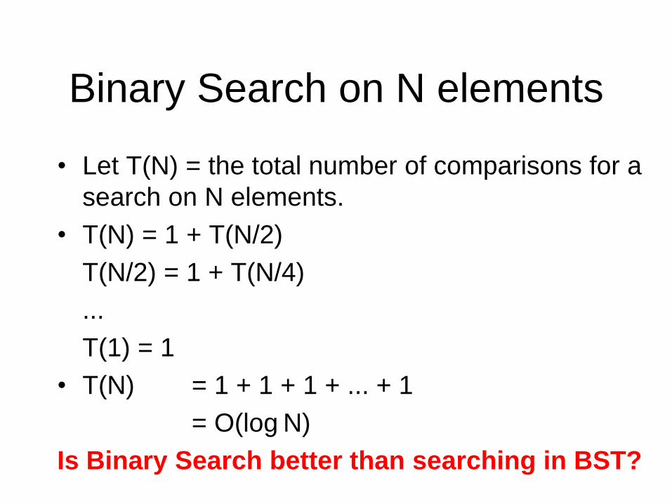
Binary Search on N elements

• Let T(N) = the total number of comparisons for a

search on N elements.

• T(N) = 1 + T(N/2)

T(N/2) = 1 + T(N/4)

...

T(1) = 1

• T(N) = 1 + 1 + 1 + ... + 1

= O(log N)

Is Binary Search better than searching in BST?

Hashing

• Data records are stored in a hash table.

• The position of a data record in the hash

table is determined by its key.

• A hash function maps keys to positions in

the hash table.

• If a hash function maps two keys to the

same position in the hash table, then a

collision occurs.

Goals of Hashing

• An insert without a collision takes O(1) time.

• A search also takes O(1) time, if the record is stored in its proper location.

• The hash function can take many forms:

- If the key k is an integer:k % tablesize

- If key k is a String (or any Object):k.hashCode() % tablesize

- Any function that maps k to a table position!

• The table size should be a prime number.

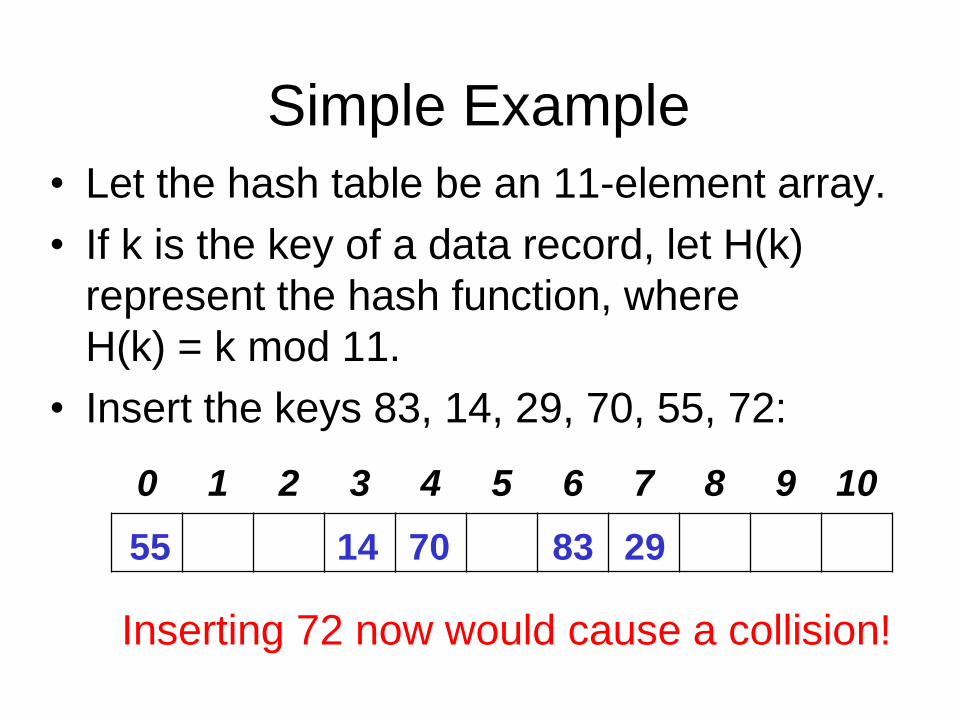
Simple Example

• Let the hash table be an 11-element array.

• If k is the key of a data record, let H(k)

represent the hash function, where

H(k) = k mod 11.

• Insert the keys 83, 14, 29, 70, 55, 72:

0 1 2 3 4 5 6 7 8 9 10

Inserting 72 now would cause a collision!

8314 297055

Collision Resolution(Chained Hashing and Open addressing)

• Linear Probing

- During insert of key k to position p:

If position p contains a different key, then examine positions p+1, p+2, etc.* until an empty position is found and insert k there.

- During a search for key k at position p:

If position p contains a different key, then examine positions p+1, p+2, etc.* until either the key is found or an unused position is encountered.

*wrap around to beginning of array if p+i> tablesize

Collision Resolution (cont’d)• Quadratic probing

If position p contains a different key, then

examine positions p+1, p+4, p+9, etc. until

either the key is found or an empty position

is encountered.

• Example: Insert additional key 72, 36, 48

using H(k) = k mod 11 and linear probing.

0 1 2 3 4 5 6 7 8 9 10

55 14 70 83 29 7236 48

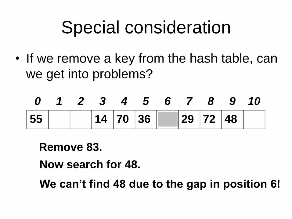
Special consideration

• If we remove a key from the hash table, can

we get into problems?

0 1 2 3 4 5 6 7 8 9 10

55 14 70 36 83 29 72 48

Remove 83.

Now search for 48.

We can’t find 48 due to the gap in position 6!

Special consideration(cont’d)

• Add another array with boolean values that

indicate whether the position is currently

used or has been used in the past.

• If a key is removed, leave the boolean value

set at true so we can search past it if

necessary.

0 1 2 3 4 5 6 7 8 9 10

55 14 70 36 83 29 72 48

T F F T T T T T T T F

Load Factor

• The load factor a of a hash table is given by

the following formula:

a = number of elements in table/size of table

• Thus, 0 < a < 1 for linear probing.

(a can be greater than 1 for other collision

resolution methods like chained hashing)

• For linear probing, as a approaches 1, the

number of collisions increases

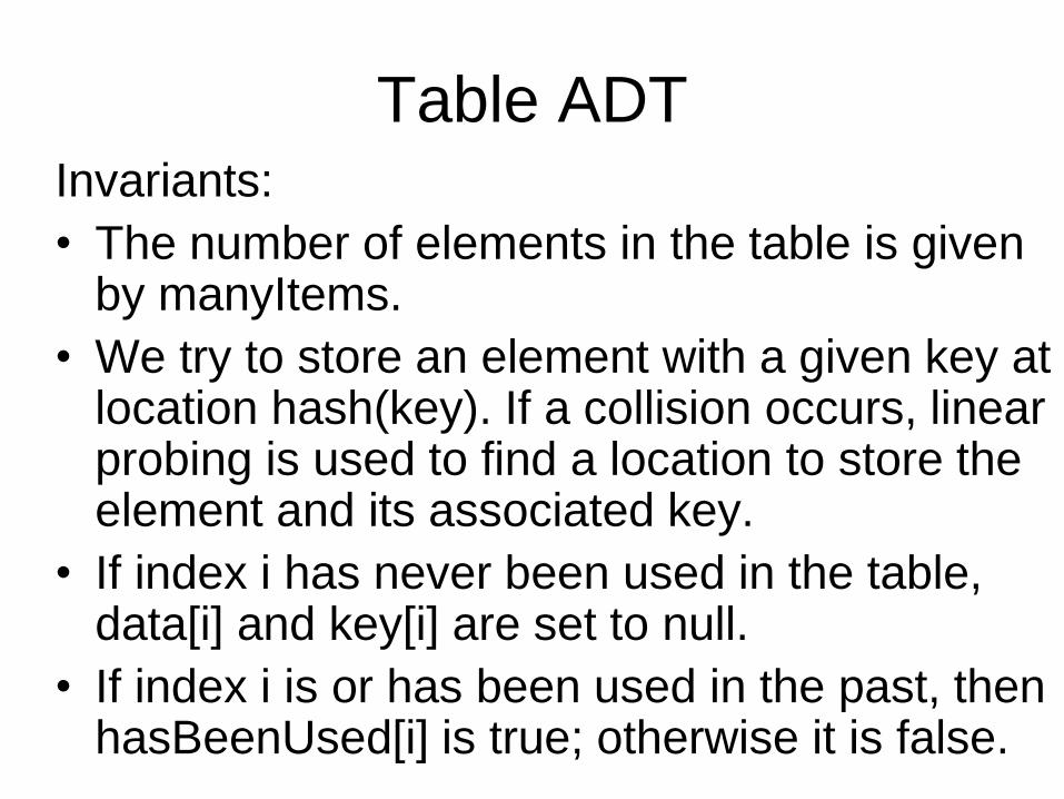
Table ADT Invariants:

• The number of elements in the table is given by manyItems.

• We try to store an element with a given key at location hash(key). If a collision occurs, linear probing is used to find a location to store the element and its associated key.

• If index i has never been used in the table, data[i] and key[i] are set to null.

• If index i is or has been used in the past, then hasBeenUsed[i] is true; otherwise it is false.

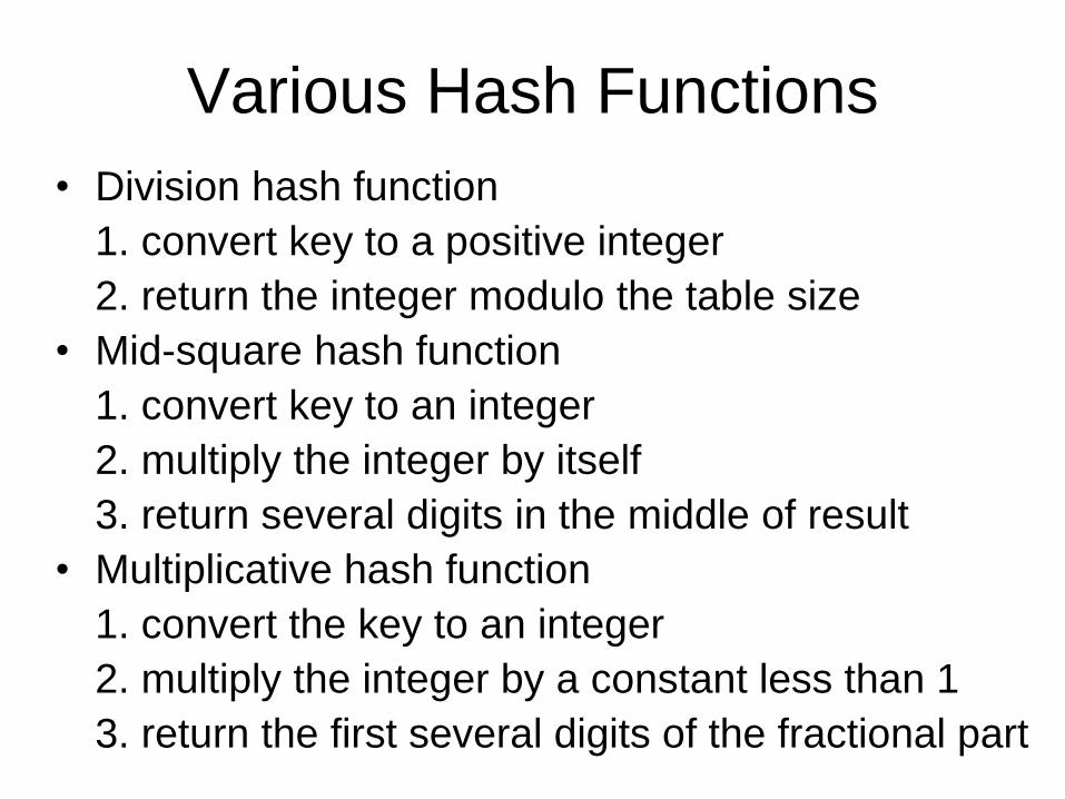
Various Hash Functions

• Division hash function

1. convert key to a positive integer

2. return the integer modulo the table size

• Mid-square hash function

1. convert key to an integer

2. multiply the integer by itself

3. return several digits in the middle of result

• Multiplicative hash function

1. convert the key to an integer

2. multiply the integer by a constant less than 1

3. return the first several digits of the fractional part

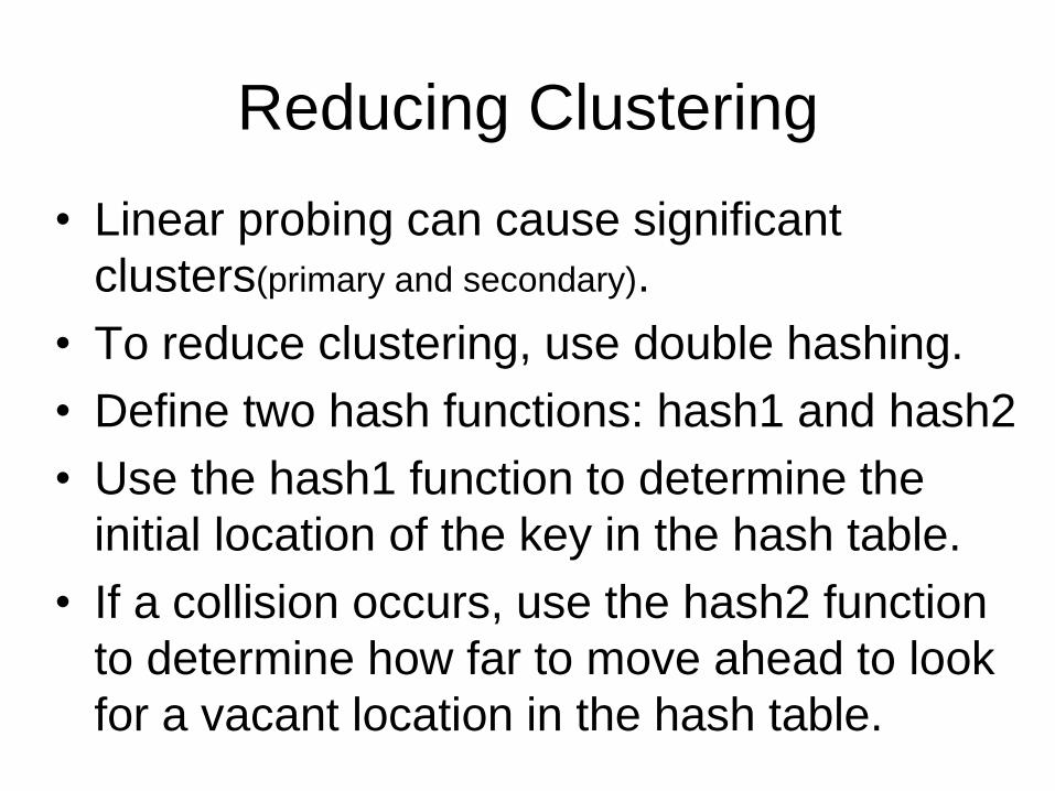
Reducing Clustering

• Linear probing can cause significant

clusters(primary and secondary).

• To reduce clustering, use double hashing.

• Define two hash functions: hash1 and hash2

• Use the hash1 function to determine the

initial location of the key in the hash table.

• If a collision occurs, use the hash2 function

to determine how far to move ahead to look

for a vacant location in the hash table.

Double Hashing Example

• H1(k) = k mod 1231H2(k) = 1+k mod 1229

• For key k = 2000: H1(k) = 769

• If location 769 is occupied, H2(k) = 772

• So we check position (769+772) mod 1231 = 310 to see if it is occupied.

• If it is, we check position (310+772) mod 1231 = 1082, etc.

• The table size is relatively prime to the value returned by the second hash function hash2.

d=gcd(H2(k),tableSize)=1

tableSize/d=1231/1=1231

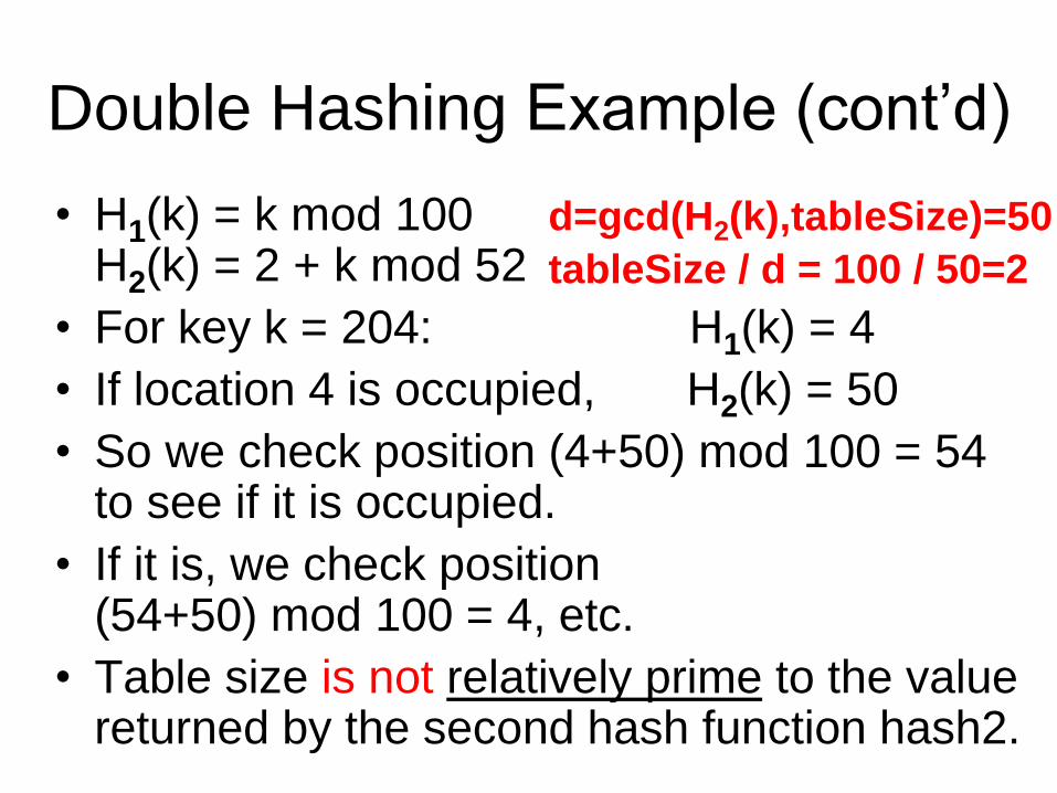
Double Hashing Example (cont’d)

• H1(k) = k mod 100H2(k) = 2 + k mod 52

• For key k = 204: H1(k) = 4

• If location 4 is occupied, H2(k) = 50

• So we check position (4+50) mod 100 = 54 to see if it is occupied.

• If it is, we check position (54+50) mod 100 = 4, etc.

• Table size is not relatively prime to the value returned by the second hash function hash2.

d=gcd(H2(k),tableSize)=50

tableSize / d = 100 / 50=2

Chained Hashing

• The maximum number of elements that can

be stored in a hash table implemented using

an array is the table size (a = 1.0).

• We can have a load factor greater than 1.0

by using chained hashing.

• Each array position in the hash table is a

head reference to a linked list of keys.

• All colliding keys that hash to an array

position are inserted to that linked list.

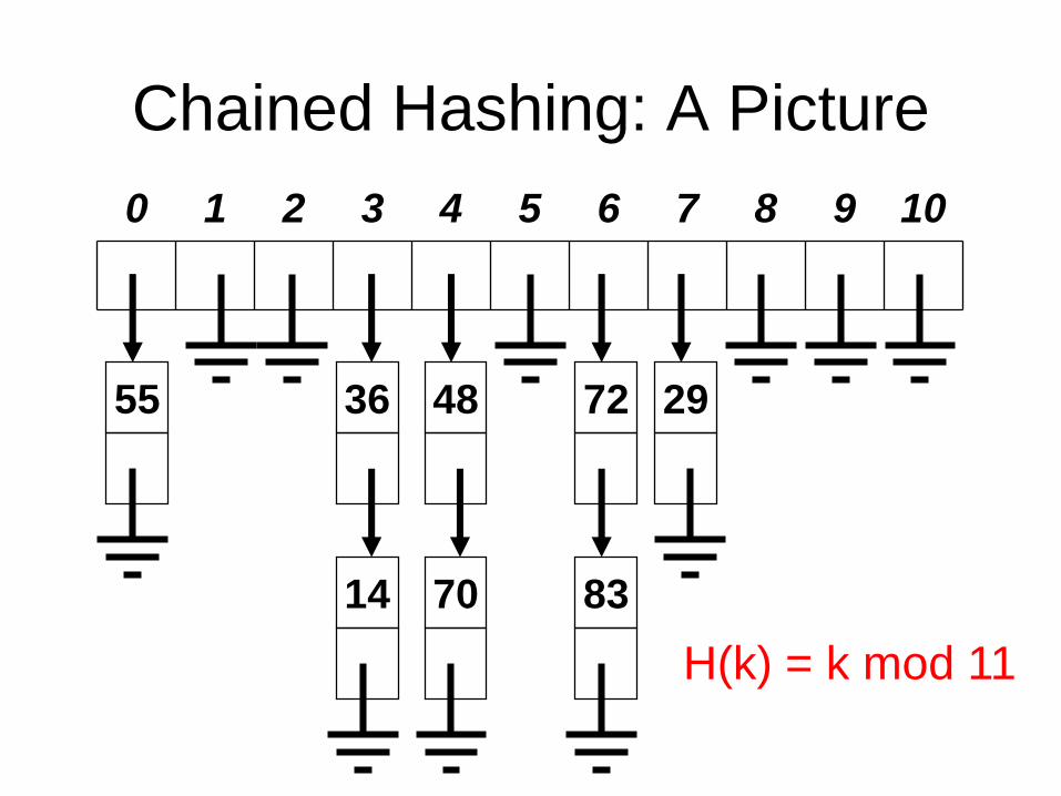
Chained Hashing: A Picture

0 1 2 3 4 5 6 7 8 9 10

36 72 294855

8314 70

H(k) = k mod 11

Average Search Time

• The average number of table elements

examined in a successful search is

approximately:

(1 + 1/(1-a)) / 2 using linear probing*

-ln(1- a) / a using double hashing*

1 + a/2 using chained hashing

*assuming a non-full hash table with no removals

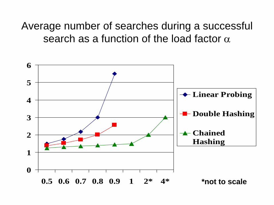
Average number of searches during a successful

search as a function of the load factor a

0

1

2

3

4

5

6

0.5 0.6 0.7 0.8 0.9 1 2* 4*

Linear Probing

Double Hashing

Chained

Hashing

*not to scale

Birthday Paradox• Probability that n people don’t have the

same birthday:

p = (364/365)*(363/365)*...*((365-n+1)/365)

• When n > 24, p < 0.5.

• This means when n > 24, chances are better that at least two people share the same birthday!

• For any hashing problem of reasonable size, we are almost certain to have collisions.