SEAKEEPING NUMERICAL ANALYSIS IN IRREGULAR WAVES … 1... · Mechanical Testing and Diagnosis ISSN...

Mechanical Testing and Diagnosis ISSN 2247 – 9635, 2013 (III), Volume 1, pp. 19-31

SEAKEEPING NUMERICAL ANALYSIS IN IRREGULAR WAVES OF A CONTAINERSHIP

Carmen GASPAROTTI, Eugen RUSU

University of Galati, ROMANIA

[email protected]

ABSTRACT In the present work, a seakeeping analysis of a containership of 139,96m length, is performed. The study includes the linear seakeeping analysis, coupled heave and pitch motions, uncoupled roll motion, in irregular waves, heading angle 0 360 deg., with Pierson-Moskowitz wave power density spectrum. The numerical seakeeping analyses are carried on with an original DYN_OSC program code based on linear seakeeping method and statistical short term prediction response method. Taking into account the specific limits of seakeeping criteria, the dynamic response statistical polar diagrams are obtained for each motion degree and the cumulative one, pointing out the influence of the ship speed and heading angle for seakeeping assessment. Keywords: numerical seakeeping analysis, dynamic response, seakeeping criteria

1. INTRODUCTION An analysis of seakeeping characteristics of a ship moving in regular waves and

irregular waves actually involves the analysis of ship behaviour in waves [1]. The evaluation of seakeeping performance of a ship largely depends on the

environmental conditions and defined criteria and this is the main reason that any comparison related to the ship speeds, the influence of heading angles, loading conditions, etc.. is a complex problem.

Seakeeping analysis is essentially a three part problem [2]: 1. estimation of the likely environmental conditions to be encountered by the vessel, 2. prediction of the response characteristics of the vessel, 3. specification of the criteria used to assess the vessel's seakeeping behaviour. This

also defines the way in which the performance of different vessels is compared. Evaluation of seakeeping performance of a ship shall be based on its oscillations in

different states of the sea that is expected to encounter during its lifetime. The procedure starts with the predicting hydrodynamic characteristics of the ship response for several speeds and heading angles. In irregular waves, short-term and long term distributions can be used to estimate the most probable maximum values of responses.

Magnitude increase movement in varying degrees of severity can then be predicted, using wave spectra representative for the selected operational sea areas. Usually, the sea

Mechanical Testing and Diagnosis, ISSN 2247 – 9635, 2013 (III), Volume 1, 19-31

20

state is described by a theoretical wave spectrum [3]. Finally, the capacity of the ship can be estimated on the basis of probability of the remaining ship movements within acceptable limits.

In this context, the objective of the present work is to analyse the ship speed and heading angle influence on maximum RMS heave, pitch, roll motion and acceleration amplitudes. The numerical seakeeping analyses based on linear seakeeping method and statistical short term prediction response method is presented in section 2 of the work.

Table 1 presents the main characteristics of the ship.

Table 1.Simplified test ship main characteristics

L[m] 139.96 [t] 17974.5

B [m] 21.8 Jx[t m2] 1067775 H [m] 9.5 Jy[t m2] 25222622 d [m] 7.335 Iy [m4] 3376696 cB 1 AW [m

2] 2637.79 Hfore[m] 6 Nsections 43 Ffore[m] 2.5 [deg.], 0360, 15 h0[m] 3.418 us[knots] 0, 5, 10, 15, 19 zg [m] 5.5 T [s] 7.40633

xg,B,F[m] 69.48 T [s] 7.34945

g [m/s2] 9.81 T [s] 9.60724

ρwater [t/m3] 1.025 symmetric CL & amidships

2. THEORETICAL BACKGROUND

This study refers to a containership and it includes a linear seakeeping analysis in

irregular waves, coupled heave and pitch motions, uncoupled roll motion, heading angle 0 360 deg., with ISSC wave power density spectrum. The seakeeping analysis from this study is carried on under the following hypotheses [4]:

- the excitation source is wave Airy model; - the motion equations are linearized; - the ship-sides are considered vertical; - the motions amplitudes are considered small; - the Lewis based hydrodynamic coefficients; - the strip theory based hydrodynamic forces [5].

In order to meet short-term statistical parameters, the authors need to know wave spectral density function. This function must be characteristic of the sea area where the ship will sail, which is not always possible, in this sense using known standard wave spectra, accepted in ocean engineering.

Spectral density functions of the dynamic response to variations of the ship have the expressions[6]: • vertical (heave):

)(,RAO)(,H,Svvvv z

2zz (1)

• pitch (pitch):

)(,RAO)(,H,Svvvv

2 (2)

• roll (roll):

)(,RAO)(,H,Svvvv

2 (3)

21 Mechanical Testing and Diagnosis, ISSN 2247 – 9635, 2013 (III), Volume 1, 19-31

Moments of the spectral density function of the dynamic response to fluctuations of the ship are:

max

0

max

0

max

0

44

44z

4z4

max

0

max

0

max

0

oozoz

d),(S)(m;d),(S)(m;d),(S)(m

d),(S)(m;d),(S)(m;d),(S)(m

(4)

Based on the spectral moments, the most probable amplitude of the motion and acceleration to the oscillation amp = RMS (root mean square) are calculated [6]: • vertical :

z0z mRMS (5)

z4z mRMSac

pvmaxz zFsFRMS (6)

g1.0RMSacmaxz

• pitch :

0mRMS

4mRMSac

)(RMSac2

LRMSac pv

g15.0RMSac;RMS2

LZrad052.03RMS maxpvmaxpv

0max

(7)

• roll :

0mRMS

4mRMSac

)(RMSac2

BRMSac sb

rad105.06RMS 0max

g15.0RMSac maxsb (8)

Table 2 presents the limit seakeeping criteria for the containership.

Tabel 2 Limit seakeeping criteria

RMSzmax=F+Fs-zpv 1.22 m not be flooded the deck at the bow

RMSaczmax 0.1 *g RMSθmax 2 gr 0.035 rad

RMSacqpvmax 0.15 *g L/2[m] 69.98 RMSfmax 6 gr 0.105 rad

RMSacfsbmax 0.15 *g B/2[m] 10.9

Based on limit values RMSmax, RMSacmax ,polar diagramas h1/3max = f(μ,us,mot.) and

Beaufort y,Bmax , for several ship speeds us, are determinated.

Relevant parameters that characterize the behavior of the ship are forecasting as response spectrum variance functions, that depend on the sea state energy spectrum and the transfer functions of the ship. In the study of seakeeping, the correct selection of wave spectrum for a particular seaway is essential [7].


22

The first step is to calculate the transfer functions of the ship response to coupled heave (3) and pitch (5) oscillations and uncoupled roll oscillations (4). They took into account a step of 15 degree between the ship and wave main directions, resulting in 13 headings. The transfer functions include the absolute ship motions and vertical, lateral and roll accelerations.

Determination of the response spectrum and statistical quantities to the dynamic analysis of the short-term dynamic response (3 heave, 5 pitch, 4 roll) was performed with the following calculation modules, which take into account of the correction spectra depending on encountering ship-wave equivalent circular frequency [6]:

- HZ35u (DYN_OSC) – calculation module of the transfer functions for coupled heave and pitch dynamic response;

- HR44u (DYN_OSC) – calculation module of the transfer functions for uncoupled roll dynamic response.

In order to calculate the transfer functions for the coupled heave (3) and pitch (5) oscillations and uncoupled roll oscillations (4) have considered the following cases:

- heading angle between the ship and wave main direction [degree]= 0, 15, 30, 45, 60, 75, 90, 105, 120, 135, 150, 165, 180;

- us ship speed [Nd]= 0, 5, 10, 15, 19 (0; 2.572; 5.144; 7.714; 9, 7736; [m/s]). When calculating the statistical significant parameters a1/3=2*RMS of the amplitude

and acceleration of the ship motion, the following programs have been used: - SH13_33U (DYN_OSC) to the heave oscillations, resulting the folder SHIP.AS3; - SH13_55U (DYN_OSC) to the pitch oscillations, resulting the folder SHIP.AS5; - SH13_44U (DYN_OSC) to the roll oscillations, resulting the folder SHIP.AS4. In addition for the roll, oscillations were also introduced as input data; initial

transverse metacentric height h0 and roll mass moment of inertia

.8/BJ 2x (9)

cosuk se (10)

gk

2 (10b)

where: ωe = encountering ship-wave equivalent circular frequency [rad/s]; ω= wave frequency [rad/s]; us= ship speed [m/s]; us=v x 0.5144; v [Nd], g=gravity acceleration [m/s2], μ= heading angle between the ship and wave main direction [degree], k=wave number [1/m].

The irregular wave Pierson-Moscowitz power density function input spectrum [6], used in this study, has the following expression:

4

fU2

g74,0

54

2

PM5.19e

f2

g fE

(11)

where fEPM - spectrum energy (m2·s or m2/Hz), f - wave frequency (Hz), 5.19U - wind

speed (m/s) at 19.5 m over the sea surface, g -gravity acceleration (m/s2), -

adimensional coefficient, =0.0081. From the PM spectrum data analysis, it was carried out the following equation:

5.19p

U2

g877.0f

(12)

Equation (12) permits to calculate 0m (the mean square of the spectrum) and from this

resutls:


2p0m f04.0H (13)

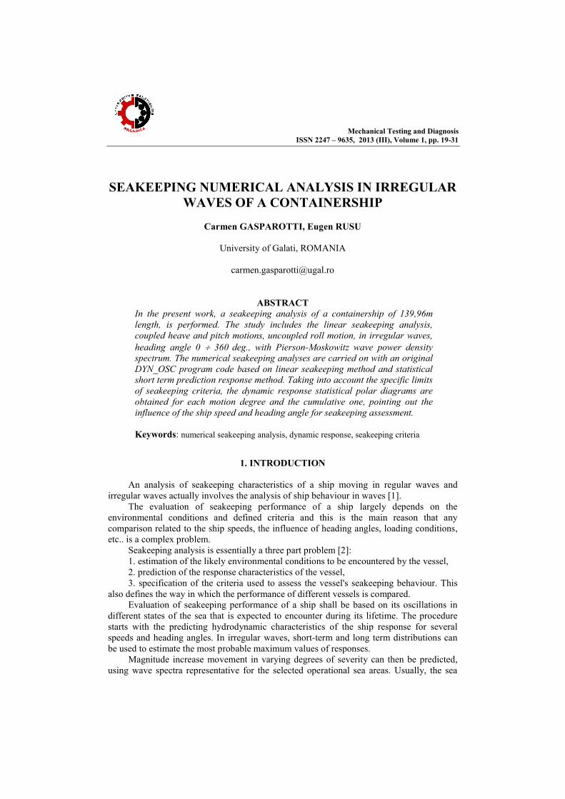
3. NUMERICAL ANALYSIS

For the ship presented in Table 1,

the numerical seakeeping analysis results are the following.

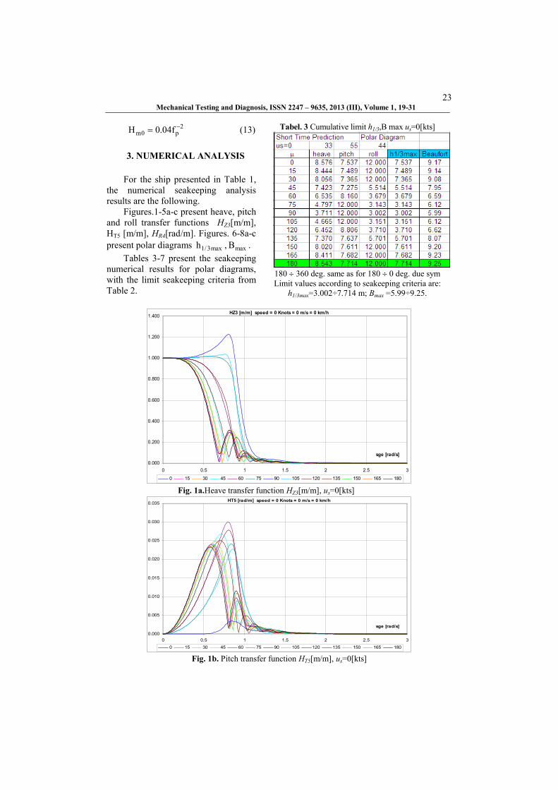
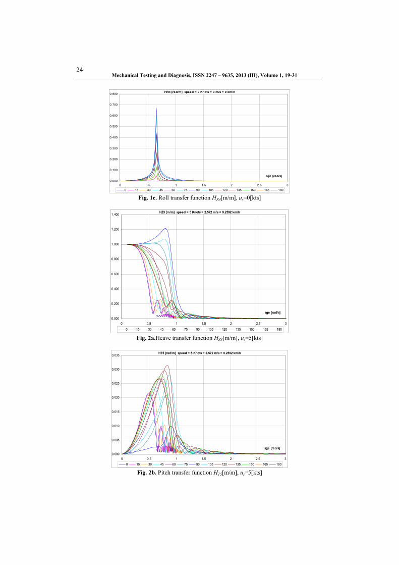
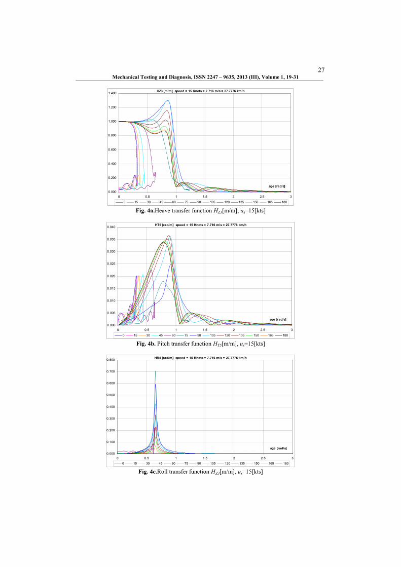
Figures.1-5a-c present heave, pitch and roll transfer functions HZ3[m/m], HT5 [m/m], HR4[rad/m]. Figures. 6-8a-c

present polar diagrams max3/1h , maxB .

Tables 3-7 present the seakeeping numerical results for polar diagrams, with the limit seakeeping criteria from Table 2.

HZ3 [m/m] speed = 0 Knots = 0 m/s = 0 km/h

0.000

0.200

0.400

0.600

0.800

1.000

1.200

1.400

0 0.5 1 1.5 2 2.5 3

sge [rad/s]

0 15 30 45 60 75 90 105 120 135 150 165 180

Fig. 1a.Heave transfer function HZ3[m/m], us=0[kts] HT5 [rad/m] speed = 0 Knots = 0 m/s = 0 km/h

0.000

0.005

0.010

0.015

0.020

0.025

0.030

0.035

0 0.5 1 1.5 2 2.5 3

sge [rad/s]

0 15 30 45 60 75 90 105 120 135 150 165 180

Fig. 1b. Pitch transfer function HT5[m/m], us=0[kts]

Tabel. 3 Cumulative limit h1/3,B max us=0[kts]

180 360 deg. same as for 180 0 deg. due sym Limit values according to seakeeping criteria are:

h1/3max=3.002÷7.714 m; Bmax =5.99÷9.25.


24

HR4 [rad/m] speed = 0 Knots = 0 m/s = 0 km/h

0.000

0.100

0.200

0.300

0.400

0.500

0.600

0.700

0.800

0 0.5 1 1.5 2 2.5 3

sge [rad/s]

0 15 30 45 60 75 90 105 120 135 150 165 180 Fig. 1c. Roll transfer function HR4[m/m], us=0[kts]

HZ3 [m/m] speed = 5 Knots = 2.572 m/s = 9.2592 km/h

0.000

0.200

0.400

0.600

0.800

1.000

1.200

1.400

0 0.5 1 1.5 2 2.5 3

sge [rad/s]

0 15 30 45 60 75 90 105 120 135 150 165 180

Fig. 2a.Heave transfer function HZ3[m/m], us=5[kts]

HT5 [rad/m] speed = 5 Knots = 2.572 m/s = 9.2592 km/h

0.000

0.005

0.010

0.015

0.020

0.025

0.030

0.035

0 0.5 1 1.5 2 2.5 3

sge [rad/s]

0 15 30 45 60 75 90 105 120 135 150 165 180



HR4 [rad/m] speed = 5 Knots = 2.572 m/s = 9.2592 km/h

0.000

0.100

0.200

0.300

0.400

0.500

0.600

0.700

0 0.5 1 1.5 2 2.5 3

sge [rad/s]

0 15 30 45 60 75 90 105 120 135 150 165 180

Fig. 2c. Roll transfer function HR4[m/m], us=5[kts]

Tabel.4 Cumulative limit h1/3,B max us=5[kts]

180 360 deg. same as for 180 0 deg. due sym

Limit values according to seakeeping criteria are: h1/3max=2.888÷8.274 m; Bmax =5.85÷9.52. HZ3 [m/m] speed = 10 Knots = 5.144 m/s = 18.5184 km/h

0.000

0.200

0.400

0.600

0.800

1.000

1.200

1.400

0 0.5 1 1.5 2 2.5 3

sge [rad/s]

0 15 30 45 60 75 90 105 120 135 150 165 180



26


0.000

0.005

0.010

0.015

0.020

0.025

0.030

0.035

0.040

0 0.5 1 1.5 2 2.5 3

sge [rad/s]

0 15 30 45 60 75 90 105 120 135 150 165 180

Fig. 3b. Pitch transfer function HT5 [m/m], us=10 [kts]


0.000

0.100

0.200

0.300

0.400

0.500

0.600

0.700

0 0.5 1 1.5 2 2.5 3

sge [rad/s]

0 15 30 45 60 75 90 105 120 135 150 165 180

Fig. 3c.Roll transfer function HZ3 [m/m], us=10 [kts]

Tabel.5 Cumulative limit h1/3,B max us=10 [kts]

180 360 deg. same as for 180 0 deg. due sym

Limit values according to seakeeping criteria are: h1/3max=2.608÷8.411 m; Bmax =5.50÷9.58



0.000

0.200

0.400

0.600

0.800

1.000

1.200

1.400

0 0.5 1 1.5 2 2.5 3

sge [rad/s]

0 15 30 45 60 75 90 105 120 135 150 165 180



0.000

0.005

0.010

0.015

0.020

0.025

0.030

0.035

0.040

0 0.5 1 1.5 2 2.5 3

sge [rad/s]

0 15 30 45 60 75 90 105 120 135 150 165 180



0.000

0.100

0.200

0.300

0.400

0.500

0.600

0.700

0.800

0 0.5 1 1.5 2 2.5 3

sge [rad/s]

0 15 30 45 60 75 90 105 120 135 150 165 180

Fig. 4c.Roll transfer function HZ3[m/m], us=15[kts]


28

Tabel 6. Cumulative limit h1/3,B max us=15 [kts] Tabel 7. Cumulative limit h1/3,B max us=19 [kts]


h1/3max=2.294÷8.326 m; Bmax =5.11÷9.54


h1/3max=2.007÷8.291 m; Bmax =4.59÷9.53


0.000

0.200

0.400

0.600

0.800

1.000

1.200

1.400

1.600

0 0.5 1 1.5 2 2.5 3

sge [rad/s]

0 15 30 45 60 75 90 105 120 135 150 165 180



0.000

0.005

0.010

0.015

0.020

0.025

0.030

0.035

0.040

0.045

0 0.5 1 1.5 2 2.5 3

sge [rad/s]

0 15 30 45 60 75 90 105 120 135 150 165 180




0.000

0.100

0.200

0.300

0.400

0.500

0.600

0.700

0.800

0 0.5 1 1.5 2 2.5 3

sge [rad/s]

0 15 30 45 60 75 90 105 120 135 150 165 180

Fig.5c. Roll transfer function HR4[m/m], us=19[kts]

Fig. 6a. Heave h1/3[m] polar diagram, us=0[kts]

Fig. 7a. Heave h1/3[m] polar diagram, us=19[kts]

Fig. 6b. Pitch h1/3[m] polar diagram, us=0[kts] Fig. 7b. Pitch h1/3[m] polar diagram, us=19[kts]


30

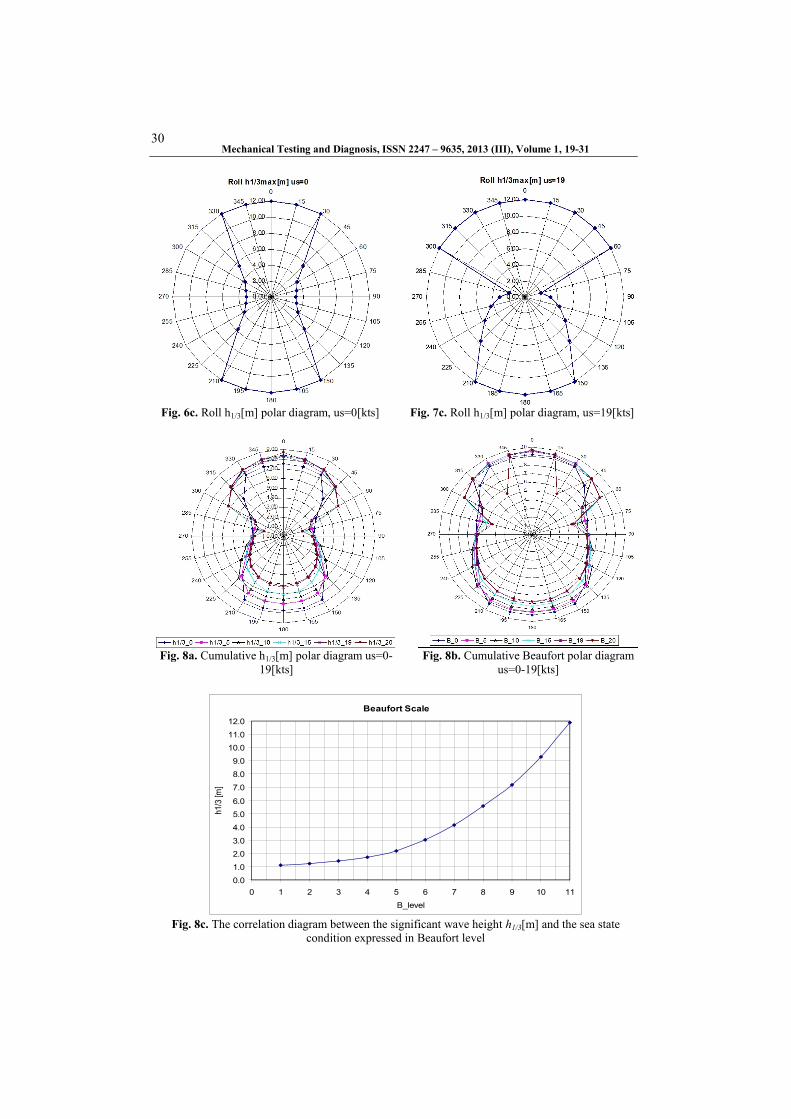
Fig. 6c. Roll h1/3[m] polar diagram, us=0[kts] Fig. 7c. Roll h1/3[m] polar diagram, us=19[kts]

Fig. 8a. Cumulative h1/3[m] polar diagram us=0-

19[kts] Fig. 8b. Cumulative Beaufort polar diagram

us=0-19[kts]

Beaufort Scale

0.0

1.0

2.0

3.0

4.0

5.0

6.0

7.0

8.0

9.0

10.0

11.0

12.0

0 1 2 3 4 5 6 7 8 9 10 11

B_level

h1/3

[m]

Fig. 8c. The correlation diagram between the significant wave height h1/3[m] and the sea state

condition expressed in Beaufort level


4. CONCLUDING REMARKS

Based on the numerical results from Section 3, it results the following conclusions. 1. The maximum significant amplitudes for heave are recorded at =90 deg., for roll

are recorded at =75 deg. for the ship speed=5-19kts and at =90 deg. for the ship speed=0kts, for pitch are recorded at =45 deg. for the ship speed=0kts, at =135 deg. for the ship speed=5, 10kts and at =120 deg. for the ship speed=15, 19kts (see Tables 3-7).

2. The maximum significant wave height limit h1/3max (polar diagrams Figs.6-8, Tables 3-7) has the following values: heave 2.833 8.701 m; pitch 4.84212 m; roll 1.91112 m; so that the most restrictive seakeeping state is recorded on the roll oscillation component.

3. Due to the ship speed increase from 0 to 19 knots, the cumulative polar diagram (Figs.8a,b) becomes asymmetric (for reference axis =90 & 270 deg.), so that the cumulative Beaufort level changes at following seas =0 (360) deg. from 9.16 to 9.72 and at head seas =180 deg. from 7.70 to 9.25. At beam sea =90 (270) deg. the cumulative Beaufort level remains unchanged 6, with no ship speed influence, being the most restrictive sea state condition.

REFERENCES

[1] McCreight K.K., Stahl R.G., 1985, Recent Advances in the Seakeeping Assessment of Ships,

Naval Engineers Journal, pp. 224-233. [2] Couser P., 2009, Seakeeping analysis for preliminary design, Fremantle, Australia: Formation

Design Systems. [3] Kadir Sarioz, Ebru Narli, 2005, Effect of criteria on seakeeping performance assessment, Ocean

Engineering, 32, pp. 1161-1173. [4] Rubanenco I., Mirciu I., Domnisoru L., 2011, Seakeeping numerical analysis in irregular

oblique waves for a simplified ship model, The Annals of “Dunarea de Jos” University of Galati Fascicle XI – Shipbuilding, pp. 45-50.

[5] Bhattacharyya R., 1978, Dynamics of marine vehicles, John Wiley & Sons Publication, New York.

[6] Domnisoru, L., 2001, Ship Dynamics. Oscillations and Vibrations (in Romanian), Technical Publishing House, Bucharest.

[7] Adi Maimun, Omar Yaakob, Md. Ahm Kamal, Ng Chee Wei, 2006, Seakeeping analysis of a fishing vessel operating in Malaysian water, Jurnal Mekanikal, no. 22, pp. 103-114.

SEAKEEPING NUMERICAL ANALYSIS IN IRREGULAR WAVES … 1... · Mechanical Testing and Diagnosis ISSN...

Documents

Transcript of SEAKEEPING NUMERICAL ANALYSIS IN IRREGULAR WAVES … 1... · Mechanical Testing and Diagnosis ISSN...