Sea Surface Temperature Biases under the Stratus Cloud ...

Sea Surface Temperature Biases under the Stratus Cloud Deck in the SoutheastPacific Ocean in 19 IPCC AR4 Coupled General Circulation Models

YANGXING ZHENG*

Cooperative Institute for Research in Environmental Sciences, University of Colorado, Boulder, Colorado

TOSHIAKI SHINODA

Naval Research Laboratory, Stennis Space Center, Mississippi

JIA-LIN LIN

Department of Geography, The Ohio State University, Columbus, Ohio

GEORGE N. KILADIS

NOAA/Earth System Research Laboratory/Physical Science Division, Boulder, Colorado

(Manuscript received 27 October 2010, in final form 27 January 2011)

ABSTRACT

This study examines systematic biases in sea surface temperature (SST) under the stratus cloud deck in the

southeast Pacific Ocean and upper-ocean processes relevant to the SST biases in 19 coupled general circu-

lation models (CGCMs) participating in the Intergovernmental Panel on Climate Change (IPCC) Fourth

Assessment Report (AR4). The 20 years of simulations from each model are analyzed. Pronounced warm SST

biases in a large portion of the southeast Pacific stratus region are found in all models. Processes that could

contribute to the SST biases are examined in detail based on the computation of major terms in the upper-

ocean heat budget. Negative biases in net surface heat fluxes are evident in most of the models, suggesting that

the cause of the warm SST biases in models is not explained by errors in net surface heat fluxes. Biases in heat

transport by Ekman currents largely contribute to the warm SST biases both near the coast and the open

ocean. In the coastal area, southwestward Ekman currents and upwelling in most models are much weaker

than observed owing to weaker alongshore winds, resulting in insufficient advection of cold water from the

coast. In the open ocean, warm advection due to Ekman currents is overestimated in models because of the

larger meridional temperature gradient, the smaller zonal temperature gradient, and overly weaker Ekman

currents.

1. Introduction

Climate in the southeast Pacific (SEP) near the coast

of Peru and Chile is controlled by complex upper-ocean,

marine boundary layer and land processes and their in-

teractions. A variety of coupled processes between the

ocean and atmosphere are involved in this tightly cou-

pled system, and the variation of the system has sig-

nificant impacts on global climate (e.g., Ma et al. 1996;

Miller 1997; Gordon et al. 2000; Xie 2004). For example,

strong winds parallel to the coast generate intense coastal

upwelling, bringing cold water to the ocean surface, which

helps to maintain the persistent stratus/stratocumulus

cloud decks by stabilizing the lower troposphere. These

persistent stratus decks have a substantial impact on the

surface energy budget in the tropics and subtropics by

reflecting sunlight back to space.

It is well known that coupled atmosphere–ocean

general circulation models (GCMs) tend to have sys-

tematic errors in the SEP region, including a warm bias

in SST and too little cloud cover (e.g., Mechoso et al.

* Current affiliation: The Florida State University, Tallahassee,

Florida.

Corresponding author address: Yangxing Zheng, Center for

Ocean–Atmospheric Prediction Studies, The Florida State Uni-

versity, 2035 E. Paul Dirac Dr., Johnson Building, Tallahassee, FL

32306-2840.

E-mail: [email protected]

1 AUGUST 2011 Z H E N G E T A L . 4139

DOI: 10.1175/2011JCLI4172.1

� 2011 American Meteorological Society

Report Documentation Page Form ApprovedOMB No. 0704-0188

Public reporting burden for the collection of information is estimated to average 1 hour per response, including the time for reviewing instructions, searching existing data sources, gathering andmaintaining the data needed, and completing and reviewing the collection of information. Send comments regarding this burden estimate or any other aspect of this collection of information,including suggestions for reducing this burden, to Washington Headquarters Services, Directorate for Information Operations and Reports, 1215 Jefferson Davis Highway, Suite 1204, ArlingtonVA 22202-4302. Respondents should be aware that notwithstanding any other provision of law, no person shall be subject to a penalty for failing to comply with a collection of information if itdoes not display a currently valid OMB control number.

1. REPORT DATE JAN 2011 2. REPORT TYPE

3. DATES COVERED 00-00-2011 to 00-00-2011

4. TITLE AND SUBTITLE Sea Surface Temperature Biases under the Stratus Cloud Deck in theSoutheast Pacific Ocean in 19 IPCC AR4 Coupled General Circulation Models

5a. CONTRACT NUMBER

5b. GRANT NUMBER

5c. PROGRAM ELEMENT NUMBER

6. AUTHOR(S) 5d. PROJECT NUMBER

5e. TASK NUMBER

5f. WORK UNIT NUMBER

7. PERFORMING ORGANIZATION NAME(S) AND ADDRESS(ES) Naval Research Laboratory,Stennis Space Center,MS,39529

8. PERFORMING ORGANIZATIONREPORT NUMBER

9. SPONSORING/MONITORING AGENCY NAME(S) AND ADDRESS(ES) 10. SPONSOR/MONITOR’S ACRONYM(S)

11. SPONSOR/MONITOR’S REPORT NUMBER(S)

12. DISTRIBUTION/AVAILABILITY STATEMENT Approved for public release; distribution unlimited

13. SUPPLEMENTARY NOTES

14. ABSTRACT This study examines systematic biases in sea surface temperature (SST) under the stratus cloud deck in thesoutheast Pacific Ocean and upper-ocean processes relevant to the SST biases in 19 coupled generalcirculation models (CGCMs) participating in the Intergovernmental Panel on Climate Change (IPCC)Fourth Assessment Report (AR4). The 20 years of simulations from each model are analyzed. Pronouncedwarm SST biases in a large portion of the southeast Pacific stratus region are found in all models.Processes that could contribute to the SST biases are examined in detail based on the computation of majorterms in the upperocean heat budget. Negative biases in net surface heat fluxes are evident in most of themodels, suggesting that the cause of the warm SST biases in models is not explained by errors in netsurface heat fluxes. Biases in heat transport by Ekman currents largely contribute to the warm SST biasesboth near the coast and the open ocean. In the coastal area, southwestward Ekman currents and upwellingin most models are much weaker than observed owing to weaker alongshore winds, resulting in insufficientadvection of cold water from the coast. In the open ocean, warm advection due to Ekman currents isoverestimated in models because of the larger meridional temperature gradient, the smaller zonaltemperature gradient, and overly weaker Ekman currents.

15. SUBJECT TERMS

16. SECURITY CLASSIFICATION OF: 17. LIMITATION OF ABSTRACT Same as

Report (SAR)

18. NUMBEROF PAGES

26

19a. NAME OFRESPONSIBLE PERSON

a. REPORT unclassified

b. ABSTRACT unclassified

c. THIS PAGE unclassified

Standard Form 298 (Rev. 8-98) Prescribed by ANSI Std Z39-18

1995; Ma et al. 1996; Gordon et al. 2000; McAvaney et al.

2001; Kiehl and Gent 2004; Large and Danabasoglu

2006; Wittenberg et al. 2006; Lin 2007). These biases

have important impacts on the simulated earth’s radia-

tion budget and climate sensitivity. Also, the accurate

prediction of low clouds over the SEP is required to

simulate the proper strength of the trade winds and the

observed SST distribution in the tropics (Ma et al. 1996;

Gordon et al. 2000).

Although the previous studies described above repor-

ted a warm SST bias in the SEP region in many coupled

GCMs (CGCMs), it is still uncertain whether a similar

bias is evident in most state-of-the-art CGCMs and to

what extent the SST biases are model dependent. Re-

cently, in preparation for the Intergovernmental Panel on

Climate Change (IPCC) Fourth Assessment Report (AR4),

many international climate modeling centers conducted

a comprehensive set of climate simulations for the twentieth

century’s climate and different climate change scenarios in

the twenty-first century. The release of the output of IPCC

AR4 CGCM simulations provided an opportunity to in-

vestigate the systematic biases in the SEP region using long-

term simulations with a variety of CGCMs. Recently, de

Szoeke and Xie (2008) found a warm SST error on the

equator near the South American coast (28S–28N, 908–

808W) in the IPCC AR4 CGCM simulations and attributed

the error to a weaker meridional wind compared to obser-

vations. In this study, we will quantify systematic SST biases

in the SEP region in these IPCC AR4 CGCM simulations

and attempt to isolate their causes.

Since the SEP climate is a tightly coupled system, in-

accurate simulations of both atmospheric and oceanic

processes and their interactions may contribute to the

SST biases. Accordingly, it is necessary to examine in-

dividual biases in the OGCMs) and the atmospheric

GCMs (AGCMs), along with the biases in the accom-

panying ocean–atmosphere feedback processes so as to

provide useful guidance on how to improve the CGCM

simulations. The importance of three-dimensional upper-

ocean processes for controlling SST in the SEP region

has been recently demonstrated by observations, and

OGCM and CGCM experiments (Colbo and Weller

2007; Shinoda and Lin 2009; Zheng et al. 2010; Toniazzo

et al. 2010). For example, Zheng et al. (2010) estimated

the annual mean heat budget using eddy-resolving OGCM

experiments and indicated the dominant role of horizon-

tal advection of upwelled cold water from the coast in

balancing the positive surface heat flux and thus main-

taining the annual mean SST in the SEP region. Using

regional model simulations in the SEP, McWilliams and

Colas (2010) and F. Colas et al. (2011, personal com-

munication) argue that the oceanic warming from sur-

face heat fluxes off Peru and Chile (700 km from the

coastline) is balanced by cooling associated with lateral

heat transport by both mean currents and eddies from the

coastal upwelling zone. Hence, the accurate simulation of

upper-ocean processes as well as air–sea fluxes is crucial

for correctly simulating SST in this region.

Deficiencies in simulating upper-ocean processes in

the SEP region have been found in some CGCM ex-

periments. For example, Large and Danabasoglu (2006)

examined the largest and potentially most important

ocean near-surface biases in the Community Climate

System Model, version 3 (CCSM3), coupled simulation

of present-day conditions. The largest mean SST biases

develop along the eastern boundaries of subtropical gyres,

including the SEP region, and the overall coupled model

response is found to be linear. Based on the subsequent

ocean-only experiment, they suggested that the cause of

the warm bias in the southeastern tropical oceans could be

traced back to inadequate coastal upwelling close to the

coast; that is, at least part of the cause was contained in the

ocean model.

Attribution of SST errors was recently investigated by

de Szoeke et al. (2010) for October climatology along

208S from 858 to 758W in 15 IPCC AR4 CGCMs using

ship observations and three gridded observation-based

surface heat flux datasets. They found that solar radia-

tion and evaporation at the surface are overestimated in

IPCC GCMs during this season. A major focus of the

present study is to identify upper-ocean processes and

surface fluxes in the entire SEP region that could be rel-

evant to SST warm biases in CGCMs. Although the data

coverage of in situ observations in the upper ocean and

air–sea fluxes in the SEP region are still sparse, global

datasets of surface fluxes [e.g., the objectively analyzed

air–sea fluxes (OAFlux), Yu and Weller (2007)] and

ocean analysis [e.g., the Simple Ocean Data Assimilation

(SODA), Carton and Giese (2008)] have been signif-

icantly improved in recent years because a variety of

satellite data are used in the analyses. Hence, it is now

feasible to evaluate the ability of CGCMs to simulate

air–sea fluxes and upper-ocean currents and temperature

compared to reasonable estimates of some quantities from

the real world. In this study, we will examine errors in

upper-ocean processes and surface fluxes in CGCMs

that could contribute to the biases in SST. Major terms

in the upper-ocean heat budget are estimated using the

output of CGCMs, and they are compared with those

from the ocean analysis and surface flux estimates based

on satellite measurements. Submesoscale eddies are not

resolved in all IPCC AR4 CGCMs, which might impact

SST biases in these models. The possible impact of re-

solving eddies in these models on the SST biases is dis-

cussed based on recent studies that include the analysis

of the data from the Variability of the American Monsoon

4140 J O U R N A L O F C L I M A T E VOLUME 24

Systems (VAMOS) Ocean–Cloud–Atmosphere–Land

Study Regional Experiment (VOCALS Rex).

2. Models and validation datasets

a. IPCC models

The analysis is based on 20-yr (1980–99) model runs of

the Climate of the Twentieth Century (20C3M) simu-

lations from 19 coupled GCMs. Table 1 shows the model

names and acronyms, their ocean model horizontal and

vertical resolutions, heat flux corrections, and which run

is employed for analysis. The resolution of the ocean

models within the stratus region is also shown. For each

model, we use 20 years of monthly mean ocean temper-

ature, salinity, three-dimensional ocean currents, surface

wind stress, sea level pressure, surface downward/upward

shortwave/longwave radiation, surface latent heat flux,

surface sensible heat flux, and near-surface meteorolog-

ical variables (wind speed at 10 m, and air temperature

and air specific humidity at 2 m).

b. SODA

The SODA methodology, the ingested data, and the

error covariance structure of both the model and the

observations are described by Carton et al. (2000a,b),

Carton and Giese (2008), and Zheng and Giese (2009).

The ocean model is based on the Los Alamos imple-

mentation of the Parallel Ocean Program (POP) (Smith

et al. 1992). The model resolution is on average 0.258

latitude 3 0.48 longitude with 40 levels in the vertical. The

model is forced with the 40-yr European Centre for

Medium-Range Weather Forecasts Re-Analysis (ERA-40)

daily atmospheric reanalysis winds (Simmons and Gibson

2002) for the 44-yr period from 1958 to 2001.

TABLE 1. List of the 19 IPCC AR4 coupled GCMs that participated in the study.

Modeling

Groups

IPCC identifier (label

in figures)

Resolutiona

(stratus)bHeat flux

correction Run

Bjerknes Center for Climate Research BCCR-BCM2.0 (bccr) 360 3 180-L33 (1 3 1) None 1

Canadian Centre for Climate Modelling and Analysis CGCMA3.1-T47 (cgcm-t47) 192 3 96-L29 (1.9 3 1.9) Yes 1

Canadian Centre for Climate Modelling and Analysis CGCMA3.1-T63 (cgcm-t63) 256 3 192-L29

(1.4 3 0.93)

Yes 1

Meteo-France/Centre National de Recherches

Meteorologique

CNRM-CM3 (cnrm) 180 3 170-L33 (2 3 1) None 1

Commonwealth Scientific and Industrial Research

Organisation

(CSIRO) Marine and Atmospheric Research

CSIRO Mk3.0 (csiro mk3.0) 192 3 189 3 L31

(1.9 3 0.93)

None 2

CSIRO Marine and Atmospheric Research CSIRO Mk3.5 (csiro mk3.5) 192 3 189 3 L31

(1.9 3 0.93)

None 1

NASA Goddard Institute for Space Studies GISS-AOM (giss-aom) 90 3 60-L31(4 3 3) None 1

NASA Goddard Institute for Space Studies GISS-ER (giss-er) 72 3 46-L33 (5 3 4) None 1

State Key Laboratory of Numerical Modeling for

Atmospheric Sciences and Geophysical Fluid

Dynamics (LASG), Institute of

Atmospheric Physics

FGOALS-g1.0 (iap) 360 3 170-L33 (1 3 1) None 1

Instituto Nazionale di Geofisica e Vulcanologia INGV-SXG (ingv) 360 3 180-L33 (1 3 1) None 1

L’Institut Pierre-Simon Laplace IPSL CM4 (ipsl) 180 3 170-L31(2 3 1) None 1

Center for Climate System Research (The University

of Tokyo), National Institute for Environmental Studies,

and Frontier Research Center for Global Change

MIROC3.2(hires)

(miroc-hires)

320 3 320-L33 (1.1 3 0.56) None 1

Center for Climate System Research (The University

of Tokyo), National Institute for Environmental Studies,

and Frontier Research Center for Global Change

MIROC3.2(medres)

(miroc-medres)

256 3 192-L33 (1.4 3 0.93) None 2

Max Planck Institute for Meteorology ECHAM5/MPI-OM (mpi) 360 3 180-L40 (1 3 1) None 1

Meteorological Research Institute MRI CGCM2.3.2 (mri) 144 3 111-L23(2.5 3 2) Yesc 1

National Center for Atmospheric Research CCSM3 (ccsm3) 320 3 395-L40 (1.1 3 0.27)d None 1

National Center for Atmospheric Research PCM (pcm) 360 3 180-L32 (1 3 1) None 3

Met Office Hadley Centre for Climate Change UKMO-HadCM3 (hadcm3) 288 3 144-L20 (1.25 3 1.25) None 1

Met Office Hadley Centre for Climate Change UKMO-HadGEM1

(hadgem1)

360 3 216-L40 (1 3 0.7)d None 1

a Resolution is about ocean model output, which is denoted by number of grid points (longitude 3 latitude) and of vertical layers (L).b Parenthesis shows horizontal resolution (longitude 3 latitude) in degrees around the stratus region (358–58S, 1008–708W).c Monthly climatological flux adjustment for heat (only 128S–128N) is used.d Grid points are not even in latitude; resolution in latitude is finer as it gets closer to the equator.


Surface heat fluxes are computed from bulk formulae

(Smith et al. 1992), with atmospheric variables from the

National Centers for Environmental Prediction–National

Center for Atmospheric Research (NCEP–NCAR) re-

analysis (Kalnay et al. 1996). The NCEP–NCAR re-

analysis information is used for the bulk formulae instead

of the ERA-40 variables throughout the experiment to

give continuity of surface forcing during periods for which

the ERA-40 winds are not available. However, the details

of surface heat flux boundary condition are relatively

unimportant in influencing the solution since near-surface

temperature observations are used to update the mixed

layer temperature. Vertical diffusion of momentum, heat,

and salt is based on a nonlocal K-profile parameterization

(KPP) (Large et al. 1994), and horizontal diffusion for

subgrid-scale processes is based on a biharmonic mixing

scheme.

The model is constrained by observed temperature

and salinity using a sequential assimilation algorithm,

which is described by Carton et al. (2000a,b) and Carton

and Giese (2008). The basic subsurface temperature

and salinity observation sets consist of approximately

7 3 106 profiles of which two-thirds have been obtained

from the World Ocean Atlas 2001 (Boyer et al. 2002;

Stephens et al. 2002) with online updates through De-

cember 2004. This dataset has been extended by the

addition of real-time temperature profile observations

from the Tropical Atmosphere Ocean/Triangle Trans-

Ocean Buoy Network (TAO/TRITON) mooring therm-

istor array and Argo floats. In addition to the temperature

profile data, a large number of near-surface temperature

observations are available, both in the form of in situ

measurements [bucket and ship-intake temperatures

from the Comprehensive Ocean–Atmosphere Data Set

(COADS) surface marine observation set of Diaz et al.

(2002)] and from satellite remote sensing. SODA used

the nighttime NOAA–National Aeronautics and Space

Administration (NASA) Advanced Very High Resolu-

tion Radiometer (AVHRR) operational SST data, which

began November 1981 and averages 25 000 samples per

week. Use of only nighttime retrievals reduces the error

due to skin temperature effects. However, the biggest

challenge in retrieving SST from an IR instrument in the

southeast Pacific Ocean is the cloud detection problem

since clouds are opaque to infrared radiation and can

effectively mask radiation from the ocean surface. Carton

et al. (2000a,b) used a bias-corrected model error co-

variance in an attempt to reduce such error. The near-

surface salinity observation set averages more than 105

observations per year since 1960 (Bingham et al. 2002).

Nearly continuous sea level information is available

from a succession of altimeter satellites beginning in

1991. Although the coverage of subsurface data in the

southeast Pacific Ocean is not as good as in other regions

of the tropics, a significant amount of satellite observations

are used in SODA, especially after 1980 (not shown). The

yearly number of observations in the southeast Pacific

(358–58S, 1408–708W) exceeds 105 after 1984. Hence, it is

likely that the SODA analysis can provide more accu-

rate estimates of mean heat advection than models with

no data assimilation. In fact, temperature and ocean

surface currents are reasonably good when compared to

World Ocean Atlas 2005 (WOA05) monthly climatology

and near-real-time ocean surface currents derived from

satellite altimeter and scatterometer data [i.e., Ocean Sur-

face Current Analyses—Real Time (OSCAR) products;

see http://www.oscar.noaa.gov/ (not shown)]. Furthermore,

horizontal heat advection in SODA is comparable to those

derived from other independent datasets, such as WOA05

and the NCEP Pacific Ocean analysis (see the appendix).

The consistency between SODA and other datasets in-

dicates that SODA is suitable for this study provided that

there are no better alternatives.

Averages of model output variables (temperature, sa-

linity, and velocity) are saved at 5-day intervals. These

average fields are remapped onto a uniform global 0.58 3

0.58 horizontal grid using the horizontal-grid spherical co-

ordinate remapping and interpolation package with second-

order conservative remapping (Jones 1999).

c. Heat flux datasets

In this study, monthly mean surface fluxes from OAFlux

(Yu and Weller 2007; Yu et al. 2008) are primarily used

for evaluating the biases of heat fluxes in CGCMs since

they are the latest—and perhaps the best—validated

datasets. Near-surface meteorological variables and SST

used to estimate the fluxes are obtained from an optimal

blending of satellite retrievals and two versions of NCEP

reanalyses [i.e., NCEP–NCAR Global Reanalysis 1

(NCEP-1) and Reanalysis 2 (NCEP-2)] and ERA-40.

NCEP-1 represents the NCEP–NCAR reanalysis proj-

ect that has produced an ongoing dataset from 1948 to

the present (Kalnay et al. 1996), and NCEP-2 represents

the NCEP–DOE reanalysis project in an effort to correct

known errors in NCEP-1 from 1979 to the present and to

improve parameterizations of some physical processes

(Kanamitsu et al. 2002). The latent and sensible fluxes are

computed from the optimally estimated near-surface at-

mospheric variables and SST using the Tropical Ocean

and Global Atmosphere Coupled Ocean–Atmosphere

Response Experiment (TOGA COARE) bulk air–sea

flux algorithm, version 3.0 (Fairall et al. 2003). Surface

latent and sensible heat fluxes as well as meteorological

variables near the surface are available from January

1958 to December 2008. Surface shortwave and longwave

radiation of OAFlux is derived from the International


Satellite Cloud Climatology Project flux dataset (ISCCP-

FD) estimates (Zhang et al. 2004) that are available from

1 July 1983. These flux estimates are compared to 107

(105 buoys and two ships) in situ flux time series, and

found to be relatively unbiased and have the smallest

mean error compared to other datasets (Yu and Weller

2007; Yu et al. 2008).

Since there are still significant uncertainties in surface

heat flux estimates (e.g., Kubota et al. 2003; Brunke et al.

2003; Chou et al. 2004; Yu et al. 2008), we also use monthly

mean heat fluxes from NCEP-1, NCEP-2, ERA-40, and

the Goddard Satellite-Based Surface Turbulent Fluxes

Version 2 (GSSTF2) for the evaluation of model surface

fluxes. Latent and sensible heat fluxes in GSSTF2 are es-

timated from satellite-derived meteorological variables

and SST with a bulk flux algorithm, including salinity and

cool-skin effects (Chou et al. 2003). Observational data-

sets and an ocean analysis dataset used for evaluating the

model simulations are summarized in Table 2.

3. SST biases

Figure 1 shows the spatial distribution of SST biases in

the southeast Pacific Ocean (358–58S, 1008–708W) from

19 IPCC AR4 coupled GCMs along with the mean SST

averaged from WOA05 monthly climatology (Antonov

et al. 2006; Locarnini et al. 2006) (shown in top left

panel). The SST biases are computed as the difference

between the model SST averaged over the period 1980

through 1999 and WOA05 SST. Warm biases in SST are

evident in most models, especially in the northern part

of the stratus region, with the greatest values near the

coast, except in the INGV and the MPI models in which

peak values are offshore. The warm SST biases are

generally weaker in the southern part of the stratus re-

gion, and cold biases are found in some models. These

latitudinal variations of SST biases are further shown in

the SST biases averaged along 1008–708W as a function

of latitude (Fig. 2). Most models have warm SST biases

north of 208S. The magnitude of the bias varies sub-

stantially from model to model, especially around 58S

(;08–58C). It should be noted that relatively small

values of SST biases in the MRI CGCM-T47 and MRI

CGCM-T63 are likely to be due to the heat flux cor-

rections (Table 1).

4. Surface heat fluxes and upper-ocean processes

Errors in both surface heat fluxes and upper-ocean

processes such as horizontal advection and upwelling

could contribute to the warm SST biases in models. In

this section, we evaluate biases in surface heat fluxes and

major terms in the heat equation in models based on the

comparison with those from surface flux datasets and

SODA described in section 2. Since large SST biases are

found mostly in the northern part of the stratus region,

the analysis is performed for the region north of 208S.

a. Surface fluxes

1) NET SURFACE HEAT FLUXES

Figure 3 shows the biases of net surface heat fluxes

from 17 IPCC AR4 coupled GCMs relative to the net

surface heat fluxes from OAFlux (top left panel) that

were averaged over the period July 1983–December

1999. Note that two models (i.e., INGV and PCM) are

not included here because surface shortwave and long-

wave fluxes from these models are not available. Also,

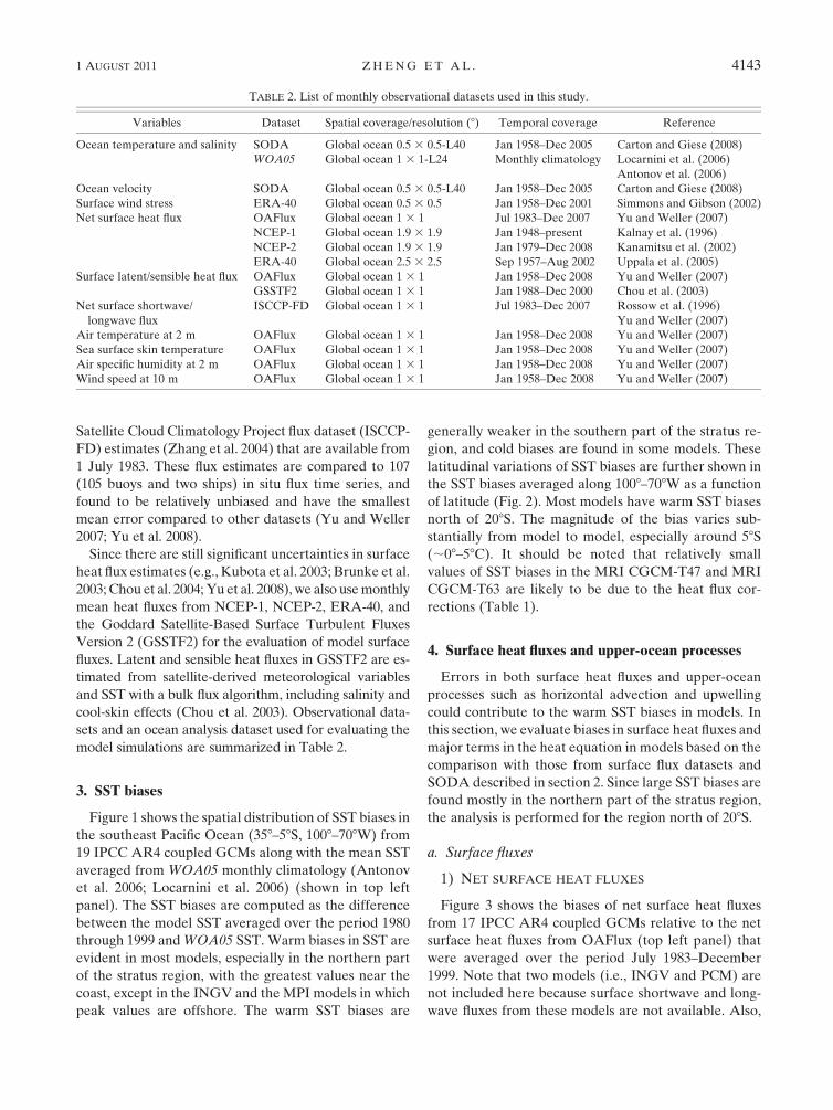
TABLE 2. List of monthly observational datasets used in this study.

Variables Dataset Spatial coverage/resolution (8) Temporal coverage Reference

Ocean temperature and salinity SODA Global ocean 0.5 3 0.5-L40 Jan 1958–Dec 2005 Carton and Giese (2008)

WOA05 Global ocean 1 3 1-L24 Monthly climatology Locarnini et al. (2006)

Antonov et al. (2006)

Ocean velocity SODA Global ocean 0.5 3 0.5-L40 Jan 1958–Dec 2005 Carton and Giese (2008)

Surface wind stress ERA-40 Global ocean 0.5 3 0.5 Jan 1958–Dec 2001 Simmons and Gibson (2002)

Net surface heat flux OAFlux Global ocean 1 3 1 Jul 1983–Dec 2007 Yu and Weller (2007)

NCEP-1 Global ocean 1.9 3 1.9 Jan 1948–present Kalnay et al. (1996)

NCEP-2 Global ocean 1.9 3 1.9 Jan 1979–Dec 2008 Kanamitsu et al. (2002)

ERA-40 Global ocean 2.5 3 2.5 Sep 1957–Aug 2002 Uppala et al. (2005)

Surface latent/sensible heat flux OAFlux Global ocean 1 3 1 Jan 1958–Dec 2008 Yu and Weller (2007)

GSSTF2 Global ocean 1 3 1 Jan 1988–Dec 2000 Chou et al. (2003)

Net surface shortwave/

longwave flux

ISCCP-FD Global ocean 1 3 1 Jul 1983–Dec 2007 Rossow et al. (1996)

Yu and Weller (2007)

Air temperature at 2 m OAFlux Global ocean 1 3 1 Jan 1958–Dec 2008 Yu and Weller (2007)

Sea surface skin temperature OAFlux Global ocean 1 3 1 Jan 1958–Dec 2008 Yu and Weller (2007)

Air specific humidity at 2 m OAFlux Global ocean 1 3 1 Jan 1958–Dec 2008 Yu and Weller (2007)

Wind speed at 10 m OAFlux Global ocean 1 3 1 Jan 1958–Dec 2008 Yu and Weller (2007)


FIG. 1. Spatial distribution of the SST biases (shading contours; 8C) relative to WOA05 from 19 IPCC AR4 coupled GCMs in the region

(358–58S, 1008–708W): (top left) SST from WOA05. Contour interval is 0.58C.


woa05:SST csiro-mk3.0 ingv mri 5"S

15"S

25"5

0 35'S

beer csiro-mk3.5 ipsl ccsm3

egem-t47 giss-aom miroe-hires pem 5'S

~:-~ 15'S -...._,o_s~

~~~ 25'S

35"S

egem-t63 giss-er hadem3 5"S

15"S

25"5

35'S

cnrm lap mp1 hadgeml

1 oo"w 9D"W so"w 7D"W 1 oo"w 9D'W so·w ?o·w 10o·w go·w so·w 7o·w 1 oo·w go·w so·w ?o·w

note that radiation from ISCCP-FD (and thus net sur-

face fluxes from OAFlux) is available only from 1 July

1983. The net surface heat fluxes from OAFlux are

positive (warming the ocean, positive downward) in the

entire region of the analysis with the magnitude ;50–

120 W m22. All models have negative biases of the net

surface heat fluxes (i.e., insufficiently warming the ocean)

in almost the entire region of the analysis. Our result is

consistent with de Szoeke et al. (2010), who compared

the estimate of surface fluxes from VOCALS Rex (along

208S in October) with those from IPCC AR4 CGCMs, in

which negative biases in net surface heat flux are found

(Fig. 10 in their paper). Positive biases are found in small

regions near the coastline in some models. The nearly

universal cold biases in net surface heat fluxes suggest

that the warm SST biases in the models are not primarily

caused by errors in net surface heat fluxes.

2) INDIVIDUAL COMPONENTS OF SURFACE HEAT

FLUXES

Biases in each component of surface heat fluxes are

further examined to identify which component con-

tributes most to negative biases of the net surface heat

fluxes in CGCMs. Figure 4 displays the biases (denoted

by ‘‘3’’) of surface latent and sensible heat fluxes,

shortwave and longwave radiation (LHF, SHF, SW, and

LW, respectively), and net surface heat fluxes averaged

over the area (208–58S, 1008–708W). The horizontal lines

denote zero biases. The biases of these components are

relative to LHF and SHF from OAFlux and SW and LW

from ISCCP-FD during July 1983–December 1999. Note

that positive (negative) values in all components indicate

warming (cooling) of the ocean. The major components

contributing to negative net surface heat flux biases are

LHF and LW. Positive biases in SW are evident in most

models, indicating too few stratus clouds over this region

(e.g., Lin 2007). Thus, biases in SW would contribute to

warm SST biases in the models. However, negative biases

in LW, LHF, and SHF are found in all models: the sum-

mation of these negative biases exceeds the amount of

positive biases in SW, resulting in negative biases in the

net surface heat flux.

Negative biases of LHF and SHF could stem from

the errors of near-surface meteorological variables and

SST as well as the use of different bulk flux algorithms.

Figure 5 shows biases of near-surface meteorological

variables averaged over the area (208–58S, 1008–708W).

The specific humidity (qa) is larger and wind speed (ws)

is smaller in most models than those from OAFlux (Figs. 5a

and 5d), which results in smaller ws(qs 2 qa) (Fig. 5e).

Hence, errors in near-surface meteorological variables do

not cause negative biases in LHF. Similarly, ws(SST 2 Ta)

is smaller than that from OAFlux in most models (Fig. 5f);

thus errors in near-surface meteorological variables do not

cause negative biases in SHF. Since errors of individual

components of heat fluxes are pronounced—particularly

FIG. 2. Biases of SST (8C) in the 19 IPCC AR4 coupled GCMs, zonally averaged along 1008–

708W as a function of latitude in the southeast Pacific Ocean. SST biases are computed relative

to WOA05 monthly climatology temperature datasets. The model period for computing model

SST biases is January 1980–December 1999.


the errors in the latent heat flux, shortwave and longwave

radiation due to a lack of clouds, and too high SST in

models—they will contribute to SST biases in IPCC models,

though the modeled net surface heat fluxes appear to be

insufficient to generate warm SST biases.

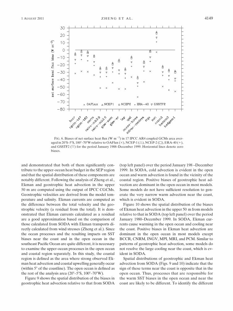
3) COMPARISON WITH OTHER SURFACE FLUX

DATASETS

Although OAFlux estimates are relatively well vali-

dated, it is difficult to determine their uncertainties be-

cause of very few in situ observations of surface fluxes

in the SEP region. To further confirm the negative biases

in model heat fluxes, we compared model fluxes with

other surface flux datasets. Net surface heat fluxes

from NCEP-1, NCEP-2, and ERA-40 are used for the

comparison. In addition to these reanalysis datasets,

satellite-based latent and sensible heat fluxes (GSSTF2)

and radiation (ISCCP-FD) are also used. Figure 6 shows

the biases of net surface heat flux averaged over the

region (208–58S, 1008–708W) relative to the five datasets

over the period January 1988–December 1999. While

there are significant differences between the datasets,

negative biases are found in all models except MRI,

suggesting that our results on surface heat flux biases are

robust—at least qualitatively.

b. Upper-ocean processes

Zheng et al. (2010) indicated that three-dimensional

upper-ocean processes, such as horizontal heat advec-

tion, play an important role in controlling the annual

mean SST in the stratus region based on the computation

of upper-ocean heat budget using OGCM experiments.

FIG. 3. Spatial distribution of the net surface heat flux biases (shading contours; W m22) relative to OAFlux from 17 IPCC AR4 coupled

GCMs in the region (208–58S, 1008–708W) of the SEP: (top left) net surface heat flux from OAFlux.


Analyses similar to those in Zheng et al. are performed

using the IPCC model outputs to examine the impact of

errors in upper-ocean processes on the SST biases.

1) HORIZONTAL HEAT ADVECTION

Horizontal heat advection integrated from the surface

to the depth z0

is defined as

Hadv 5 2

ð0

z0

rCpV � $hT dz 5 2

ð0

z0

rCp

�u

›T

›x1 y

›T

›y

�dz,

where r is the density of seawater; Cp is the specific

heat capacity of seawater at constant pressure; V is the

horizontal velocity vector, which is ui 1 yj with u and y

their components in the zonal and meridional direction,

respectively; and $h

is horizontal gradient vector, de-

fined as ›/›xi 1 ›/›yj. Horizontal heat advection in the

upper 50 m from 19 IPCC AR4 coupled GCMs is cal-

culated for the period January 1980–December 1999 and

is compared with that from SODA.

The spatial distribution of the biases in horizontal

heat advection relative to SODA is shown in Fig. 7. Cold

advection is found in most of the stratus region in SODA

(top-left panel in Fig. 7). In many models, positive

(warm) biases of horizontal heat advection are evident

in most of the region, suggesting that these biases largely

contribute to the warm SST biases in most models. How-

ever, positive biases are not dominant in some models such

FIG. 4. Biases of (a) LHF, (b) SHF, (c) net SW and (d) net LW at the ocean surface, and

(e) net surface heat flux from 17 IPCC AR4 coupled GCMs averaged in 208–58S, 1008–708W: all

fluxes and radiation (W m22). Biases are computed relative to the OAFlux monthly estimates

during July 1983–December 1999. Horizontal lines denote zero biases.


as BCCR, CNRM, INGV, and MPI. The area-average

biases in each model are shown in Fig. 8. While zonal

currents (u) in most models are weaker relative to that

(24.6 cm s21) in SODA, meridional currents (y) in

most models are slightly greater than that (21.6 cm s21)

in SODA. However, the zonal gradient of temperature

(2dT/dx) is underestimated relative to 0.233 K (100 km)21,

and the meridional gradient of temperature (2dT/dy) is

overestimated relative to SODA [20.035 K (100 km)21].

Thus, the zonal cold heat advection in most models is

underestimated relative to SODA (217 W m22), and

the meridional warm heat advection in models can be

weaker or stronger than that (9 W m22) in SODA, with

smaller errors than the zonal cold heat advection. There-

fore, the errors in zonal cold advection appear to be the

primarily source of warm SST biases in this region in most

models.

2) RELATIVE ROLES OF GEOSTROPHIC AND

EKMAN HEAT TRANSPORTS

Zheng et al. (2010) examined heat transport due to both

Ekman and geostrophic currents in OGCM experiments

FIG. 5. Biases of (a) surface air specific humidity at 2 m (qa, g kg21), (b) difference between

the saturation and air specific humidity (qs, g kg21), (c) difference between SST and air tem-

perature at 2 m (SST 2 Ta, 8C), (d) wind speed (m s21) at 10 m, (e) ws (qs 2 qa) (m s21 g kg21),

and (f) ws (SST 2 Ta) (m s21 8C) in 17 IPCC AR4 coupled GCMs area averaged in 208–58S,

1008–708W. Biases are computed relative to atmospheric and oceanic variables from the OAFlux

monthly estimates during July 1983–December 1999; horizontal lines denote zero biases.


and demonstrated that both of them significantly con-

tribute to the upper-ocean heat budget in the SEP region

and that the spatial distribution of these components are

notably different. Following the analysis of Zheng et al.,

Ekman and geostrophic heat advection in the upper

50 m are computed using the output of IPCC CGCMs.

Geostrophic velocities are derived from the model tem-

perature and salinity. Ekman currents are computed as

the difference between the total velocity and the geo-

strophic velocity (a residual from the total). It is dem-

onstrated that Ekman currents calculated as a residual

are a good approximation based on the comparison of

those calculated from SODA with Ekman transports di-

rectly calculated from wind stresses (Zheng et al.). Since

the ocean processes and the resulting impacts on SST

biases near the coast and in the open ocean in the

southeast Pacific Ocean are quite different, it is necessary

to examine the upper-ocean processes in the open ocean

and coastal region separately. In this study, the coastal

region is defined as the area where strong observed Ek-

man heat advection and coastal upwelling generally occur

(within 58 of the coastline). The open ocean is defined as

the rest of the analysis area (208–58S, 1008–708W).

Figure 9 shows the spatial distribution of the biases in

geostrophic heat advection relative to that from SODA

(top left panel) over the period January 198 –December

1999. In SODA, cold advection is evident in the open

ocean and warm advection is found in the vicinity of the

coastal region. Positive biases of geostrophic heat ad-

vection are dominant in the open ocean in most models.

Some models do not have sufficient resolution to gen-

erate the very narrow warm advection near the coast,

which is evident in SODA.

Figure 10 shows the spatial distribution of the biases

of Ekman heat advection in the upper 50 m from models

relative to that in SODA (top left panel) over the period

January 1980–December 1999. In SODA, Ekman cur-

rents cause warming in the open ocean and cooling near

the coast. Positive biases in Ekman heat advection are

dominant in the open ocean in most models except

BCCR, CNRM, INGV, MPI, MRI, and PCM. Similar to

patterns of geostrophic heat advection, some models do

not resolve the large cooling near the coast, which is ev-

ident in SODA.

Spatial distributions of geostrophic and Ekman heat

advection from SODA (Figs. 9 and 10) indicate that the

sign of these terms near the coast is opposite that in the

open ocean. Thus, processes that are responsible for

the warm SST biases in the open ocean and near the

coast are likely to be different. To identify the different

FIG. 6. Biases of net surface heat flux (W m22) in 17 IPCC AR4 coupled GCMs area aver-

aged in 208S–58S, 1008–708W relative to OAFlux (3), NCEP-1 (4), NCEP-2 (u), ERA-40 (1),

and GSSTF2 (,) for the period January 1988–December 1999. Horizontal lines denote zero

biases.


processes in these regions, further analyses are per-

formed separately for the coastal region and the open

ocean.

Figure 11 shows the biases in geostrophic and Ekman

velocities and heat advection in CGCMs averaged over

the entire area of the analysis (208–58S, 1008–708W), the

coastal region, and the open ocean. These biases are

computed relative to the averages of these quantities

from SODA, shown in Table 3. In SODA, geostrophic

currents cause warming (cooling) in the coastal (open

ocean) region. In contrast, Ekman currents cause cool-

ing (warming) in the coastal (open ocean) region. The

time-mean cooling (238 W m22) in the coastal region

from Ekman currents is much larger than the time-mean

warming (14 W m22) from geostrophic currents. In most

models, the magnitude of biases in the area-averaged

Ekman heat advection is much larger than that of geo-

strophic heat advection for both the coastal region and

open ocean. The area-average Ekman heat advection

has relatively large positive biases (warming the ocean),

both in the coastal region (ranging from 20 to 80 W m22)

and open ocean (ranging from 5 to 25 W m22). Small

positive biases (from 0 to 10 W m22) in geostrophic heat

advection are found in the open ocean for most models,

while negative biases from about 220 to 230 W m22 are

found in the coastal region.

To further examine how these biases are generated,

geostrophic and Ekman currents and temperature from

each model are described in Figs. 12 and 13, respec-

tively. In the open ocean, northwestward geostrophic

FIG. 7. Spatial distribution of the biases in horizontal heat advection (shading contours; W m22) in the upper 50 m from 19 IPCC AR4

coupled GCMs. The bias of model horizontal heat advection is relative to that from SODA over the period January 1980–December 1999.

(top left) Horizontal heat advection in the upper 50 m.


currents generally bring cold water near the coast to the

open ocean (top left panel in Fig. 12). Most models

generate a similar distribution of geostrophic currents

and temperature, and the biases in currents are small

(Fig. 11c), resulting in relatively small positive biases of

geostrophic heat advection in the open ocean. In the

coastal region, geostrophic currents are overestimated

in most models but negative biases in heat advection are

evident (Fig. 11b) because most models do not resolve

large warming due to geostrophic currents right near the

coast, which is evident in SODA (Fig. 9).

Southwestward Ekman currents bring warmer water

from low to higher latitude (top left panel in Fig. 13), and

thus Ekman transport provide warming in most of the

area in the open ocean. Since the angles between the di-

rection of Ekman currents and the isotherms in the open

ocean are generally smaller than those for geostrophic

currents, the magnitude of Ekman heat advection in the

upper 50 m is comparable to that of geostrophic heat

advection even though the Ekman currents in this layer

are much stronger (Table 3). In contrast to the relation

between the direction of Ekman currents and isotherms in

SODA, the isotherms in models are more zonal in the

open ocean and thus the Ekman currents can affect SST

warm biases in two ways. Although the Ekman currents

tend to bring cold water from the coastal region to the

FIG. 8. Biases of (a) velocity (u, y: cm s21), (b) horizontal temperature gradient [2dT/dx, 2dT/

dy: K (100 km)21], and (c) horizontal heat advection and its zonal and meridional components

(W m22) in the upper 50 m from 19 IPCC AR4 coupled GCMs averaged in 208–58S, 1008–708W.

Biases are computed relative to those from SODA during the period January 1980–December

1999; ‘‘3’’ denotes the biases of variables in the zonal direction (u, dT/dx, 2rCpudT/dx), ‘‘D’’

denotes the biases of variables in the meridional direction (y, 2dT/dy, 2rCp ydT/dy), and ‘‘1’’

denotes the biases of total horizontal heat advection. Horizontal lines denote zero biases.


open ocean less efficiently, they also tend to bring warmer

water to higher latitude more efficiently than observed

even though those currents are relatively weak in the

models (Fig. 11f). Hence, overall positive (warm) biases in

Ekman heat advection are generated in the open ocean.

These large warm biases in Ekman heat advection along

with small warm biases in geostrophic heat advection in

the open ocean (Fig. 11c) cause SST warm biases. In the

coastal region, Ekman currents cause cooling because

they advect cold upwelled water in the offshore direction

(top left panel in Fig. 13). Since Ekman currents in the

coastal region are underestimated in most models (Fig.

11e) and the large cooling effect of Ekman transport

(which is evident in SODA) is not well resolved in most

models (Fig. 10), the cooling due to advection is reduced,

resulting in positive biases of Ekman heat advection.

3) VERTICAL HEAT ADVECTION AND

COASTAL UPWELLING

Figures 14c and 14f show the vertical advection term

defined as 2rCpwdT/dz (W m22) in the upper 50 m for

the coastal region and the open ocean. While no sys-

tematic bias of this term is found in the coastal region,

significant cold biases are evident in the open ocean. The

errors in downward velocity and the resultant heat ad-

vection may be partly responsible for the cold biases in

the open ocean. In the coastal region, upwelling is overly

weak in most models (Fig. 14d). However, because of the

overly large temperature gradient in some models (Fig.

14e), these errors compensate and systematic biases are

not found (Fig. 14f). Also, it is not clear whether vertical

heat advection in the upper 50 m is directly related to

FIG. 9. As in Fig. 7 but for geostrophic heat advection (W m22).


SSTs in the coastal region since the mixed layer depth is

generally shallower than 50 m and thus large heat ad-

vection around 50 m may not directly influence SSTs.

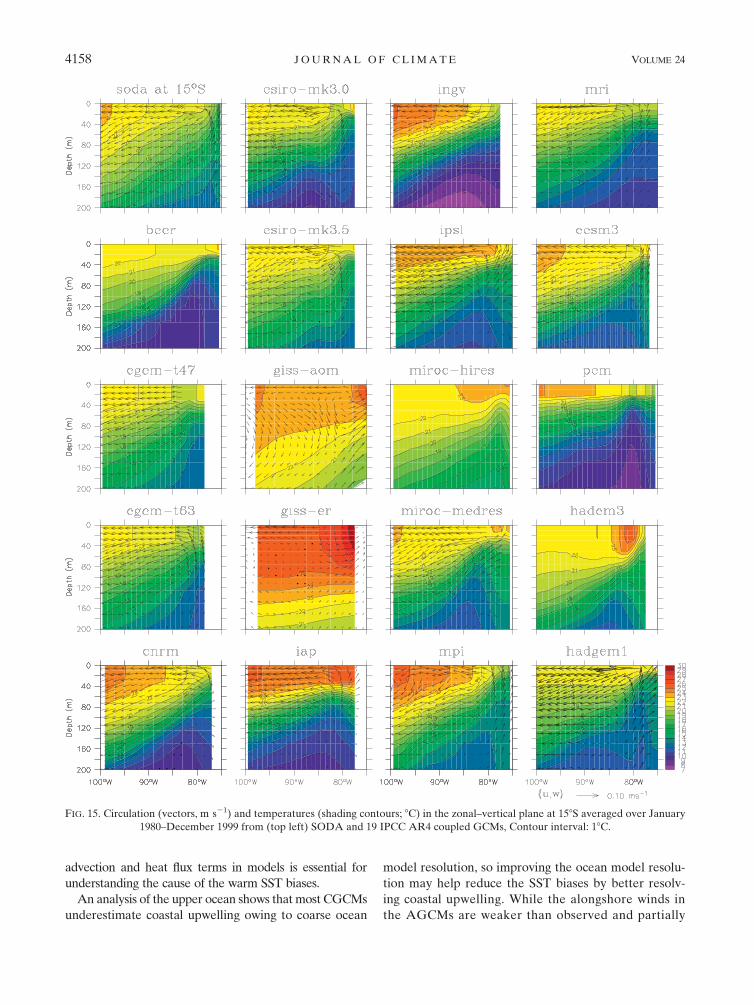
To further examine the influence of vertical heat ad-

vection on SSTs, the circulation and temperature in the

zonal–vertical plane are described. Figure 15 shows the

zonal circulation and temperature along 158S averaged

over January 1980–December 1999 from SODA and

CGCMs. Strong coastal upwelling occurs within 38–58 off-

shore in SODA. This cold upwelled water is then trans-

ported away from the coast by the mean currents. The

coastal upwelling is underestimated in most models, and

temperature profiles near the coast suggest that cold sub-

surface water affects SSTs less than those in SODA. This is

further demonstrated in the depth of the 188C isotherm

along 158S (Fig. 16). While 188C isotherms are shallower in

most models than those in SODA west of 788W, the up-

welling is not strong enough to bring water colder than

188C to the surface at the coast. The upwelling zone is

broader than in SODA in most models, which can also

influence SST in the open ocean through the vertical heat

advection term, but, overall, the magnitude is much smaller

than horizontal heat advection (Figs. 11 and 14). Similar

results are found at other latitudes between 108 and 208S.

The too broad and weak upwelling could be due to

a combination of the coarse horizontal resolution of ocean

models (Table 1) and underestimates of alongshore winds.

Figure 17 shows the strength of alongshore wind stress in

CGCMs compared to that in SODA. All models have

weaker alongshore wind stresses at most latitudes. Hence,

the relation between biases in upwelling and alongshore

winds is consistent. However, it is difficult to identify the

FIG. 10. As in Fig. 7 but for Ekman heat advection (W m22).


ultimate sources of these biases as a variety of processes in

the atmosphere and ocean as well as air–sea feedback are

involved in determining them in CGCMs.

5. Discussion

This study focuses on identifying the errors of upper-

ocean processes and air–sea fluxes in CGCMs that could

contribute to SST biases in the SEP region. It is worth

reemphasizing that the net causes of these SST biases

are likely ultimately determined by a combination of

atmospheric, land, and oceanic processes, along with

air–sea feedback processes that could amplify the errors

in both AGCM and OGCM components. For example,

strong alongshore winds at the coast of Chile and Peru

are primarily caused by the great height of the Andes

FIG. 11. Biases of geostrophic heat advection (denoted by ‘‘3’’; W m22) and biases of geostrophic current speed

(denoted by ‘‘4’’; cm s21) averaged over (a) 208–58S, 1008–708W, (b) the coastal region between 208 and 58S, and

(c) the open ocean in the upper 50 m from 19 IPCC AR4 coupled GCMs. (d)–(f) As in (a)–(c) but for biases of

Ekman heat advection and current speed. Biases of these variables are relative to those from SODA during January

1980–December 1999; the ordinate on the left (right) side of the panel indicates biases in heat advection (velocity).

Coastal region is defined as the area 58 from the coastline. Horizontal lines denote zero biases.


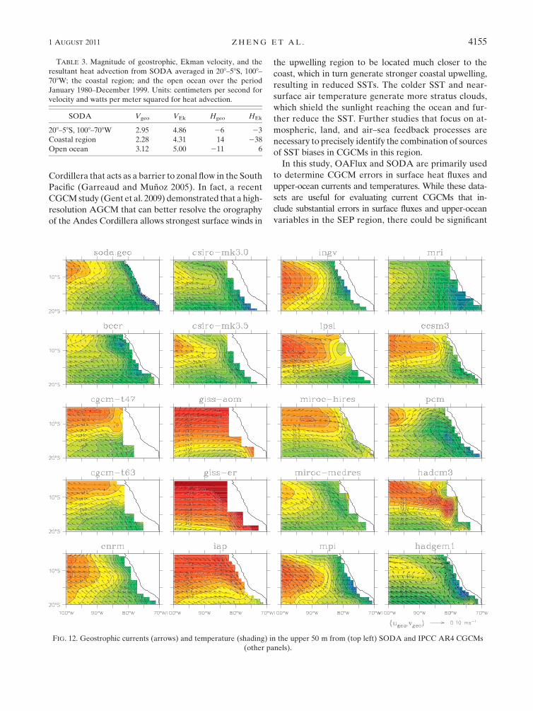
Cordillera that acts as a barrier to zonal flow in the South

Pacific (Garreaud and Munoz 2005). In fact, a recent

CGCM study (Gent et al. 2009) demonstrated that a high-

resolution AGCM that can better resolve the orography

of the Andes Cordillera allows strongest surface winds in

the upwelling region to be located much closer to the

coast, which in turn generate stronger coastal upwelling,

resulting in reduced SSTs. The colder SST and near-

surface air temperature generate more stratus clouds,

which shield the sunlight reaching the ocean and fur-

ther reduce the SST. Further studies that focus on at-

mospheric, land, and air–sea feedback processes are

necessary to precisely identify the combination of sources

of SST biases in CGCMs in this region.

In this study, OAFlux and SODA are primarily used

to determine CGCM errors in surface heat fluxes and

upper-ocean currents and temperatures. While these data-

sets are useful for evaluating current CGCMs that in-

clude substantial errors in surface fluxes and upper-ocean

variables in the SEP region, there could be significant

TABLE 3. Magnitude of geostrophic, Ekman velocity, and the

resultant heat advection from SODA averaged in 208–58S, 1008–

708W; the coastal region; and the open ocean over the period

January 1980–December 1999. Units: centimeters per second for

velocity and watts per meter squared for heat advection.

SODA Vgeo VEk Hgeo HEk

208–58S, 1008–708W 2.95 4.86 26 23

Coastal region 2.28 4.31 14 238

Open ocean 3.12 5.00 211 6

FIG. 12. Geostrophic currents (arrows) and temperature (shading) in the upper 50 m from (top left) SODA and IPCC AR4 CGCMs

(other panels).


uncertainties in these analyses. It has been difficult to val-

idate these datasets since there were few in situ measure-

ments of upper-ocean and surface fluxes in the SEP region

until recently. Intensive in situ observations of the upper-

ocean and atmospheric boundary layer, including air–sea

fluxes, were conducted in fall 2008 as part of VOCALS

(Wood et al. 2007). A substantial amount of data collected

during the VOCALS REx would be useful to evaluate

a variety of surface flux datasets and ocean analysis and to

validate various schemes used in the analysis, such as the

bulk flux algorithm. Hopefully, these global datasets will be

further improved after the validation and evaluation of

the analyses based on comparison using the data from

VOCALS REx as well as other observations.

Since none of the IPCC AR4 coupled GCMs resolve

mesoscale and submesoscale eddies because of their

coarse horizontal resolution, the role of eddy activity in

the warm SST biases could not be investigated in this

study. The precise role of eddies in the heat budget of

the SEP is still controversial. For example, recent in-

dependent high-resolution modeling studies (Zheng

et al. 2010; Toniazzo et al. 2010) indicated that long-term

mean area-averaged eddy heat flux divergence is small

over the SEP region. Conversely, McWilliams and Colas

(2010) and F. Colas et al. (2011, personal communication)

examine the heat balance in the Peru–Chile Current

System (PCS) using regional ocean models (ROMs),

and show that both the total mean-flow advection and

eddy heat flux are necessary to sustain the oceanic cooling

in the PCS. It should be noted that the domain of their

analysis is limited to a region in the PCS (700 km from

the coastline), which is much smaller than the scale of

FIG. 13. As in Fig. 12 but for Ekman currents.


the stratus cloud deck and warm SST biases in the SEP.

This result is consistent with our previous study that

shows the importance of eddy heat flux near the coast

(Fig. 12 in Zheng et al. 2010).

More recent studies suggest that eddies can contribute

to lowering the upper ocean’s heat content (and hence

SST) by bringing a cold, fresh Pacific intermediate layer

closer to the surface. Vertical mixing associated with

double diffusion between the eastern South Pacific In-

termediate Water and the surface layer appears to play

an essential role in maintaining the upper ocean’s heat

content and salt balance based on the analysis of VOCAL

REx data (e.g., Straneo et al. 2010; Zappa et al. 2010).

Despite the controversies about the role of eddies in the

maintenance of cold waters in the SEP, all recent studies

described above affirm the leading importance of heat ad-

vection in controlling SSTs in this region. Since it is likely

that horizontal and vertical heat advection significantly

contribute to maintaining cold SSTs—at least for the scale

of the stratus cloud deck in the SEP—the evaluation of

FIG. 14. (a) Vertical velocity (w, 1024 cm s21) averaged in the upper 50 m, (b) 2dT/dz [K (10 m)21] averaged in

the upper 50-m depth, and (c) 2rCpwdT/dz (W m22) integrated in the upper 50 m and then averaged in the open-

ocean area from SODA and 15 IPCC AR4 coupled GCMs. (d)–(f) As in (a)–(c) but for those averaged in the coastal

region. Horizontal solid lines denote zero biases; horizontal dashed lines denote zero values.


advection and heat flux terms in models is essential for

understanding the cause of the warm SST biases.

An analysis of the upper ocean shows that most CGCMs

underestimate coastal upwelling owing to coarse ocean

model resolution, so improving the ocean model resolu-

tion may help reduce the SST biases by better resolv-

ing coastal upwelling. While the alongshore winds in

the AGCMs are weaker than observed and partially

FIG. 15. Circulation (vectors, m s21) and temperatures (shading contours; 8C) in the zonal–vertical plane at 158S averaged over January

1980–December 1999 from (top left) SODA and 19 IPCC AR4 coupled GCMs, Contour interval: 18C.


soda at 15°S csiro-mk3.0 ingv mri 0

40

~ 80 £

g. 120 D

160

200

beer csiro-mk3.5 ipsl ecsm3 0

40

E' 80 £

g. 120 D

160

200

cgcm-t47 giss-aom miroc-hires pcm 0

40

~ 80 .c

1} 120 D

160

200

cgcm-t63 g1ss-er miroe-medres hadcm3 0

40

~ 80 £

g. 120 D

160

200

cnrm iap mpi hadgeml 0

40

E' 80 .c

g. 120 D

160

200

100"1'1 9D"W BO"W 100"W 9D"W 80"W 100"W 90"1'1 80"W lDD"W 90"W BO"W (u,w) ------;;. 0.10ms-1

responsible for the weaker upwelling, the horizontal res-

olution in the OGCMs is not adequate to resolve strong

and narrow upwelling. Accordingly, improving the hori-

zontal resolution in the OGCM component may reduce

warm SST biases in the coastal region. Also, if more cold

water is upwelled at the coast, warm SST biases in the

open ocean would also be reduced by horizontal advec-

tion of this water away from the coast.

The result also shows that cold water (less than 188C)

is upwelled to around 30–40-m depth in many models

(Figs. 15 and 16), but this does not significantly affect

SST, possibly because mixing in the upper layer (i.e.,

above 40 m) is not sufficiently strong. The improvement

of mixing schemes is a major challenge in ocean mod-

eling, but this is a worthwhile endeavor and is likely to

also reduce SST biases. For example, OGCM and one-

dimensional ocean model experiments could be performed

to examine the sensitivity of the upper-ocean tempera-

ture and SST near the coast to different mixing schemes.

Comparisons with high quality and fine resolution data in

the upper ocean obtained during VOCALS REx would

be very useful for such studies.

The underestimated alongshore winds in the AGCM

component of IPCC AR4 models could be partly at-

tributed to overestimated precipitation in the SEP re-

gion (M. Davis et al. 2011, personal communication).

Although deep convection is rarely observed in the

SEP, many IPCC AR4 models produce substantial

precipitation in this region, which is in turn tied to the

double intertropical convergence zone (ITCZ) problem

(Mechoso et al. 1995; Lin 2007; de Szoeke and Xie 2008).

Excess precipitation lowers the sea level pressure because

the release of latent heat due to unrealistically high pre-

cipitation heats the atmosphere locally. Thus, the sub-

tropical high is weakened, leading to weaker alongshore

winds. Lin (2007) hypothesized that the overestimation of

tropical precipitation in IPCC AR4 models is caused by

their lack of the observed self-suppression processes in

tropical convection, such as the sensitivity of convective

updrafts to lower tropospheric moisture, the cooling and

drying of the boundary layer by convective downdrafts,

and the warming and drying of the lower troposphere by

mesoscale downdrafts. Including these processes in

model deep-convection schemes may help lead to a more

realistic upper-ocean state by reducing the excessive

precipitation in the SEP region and enhancing the sub-

tropical high and alongshore winds.

6. Summary

This study investigates processes in the upper ocean

and air–sea fluxes that could contribute to systematic

SST biases under stratus cloud decks in the southeast

Pacific in 19 IPCC AR4 coupled GCMs. Surface fluxes

and upper-ocean variables from the output of CGCMs

are analyzed and compared with surface flux estimates

FIG. 16. Depth of the 188C isotherm along 158S averaged over the period January 1980–

December 1999 from SODA and 17 IPCC AR4 coupled GCMs. Two models (GISS-AOM and

GISS-ER) are excluded because of their extreme values (see also Fig. 15).


(OAFlux) and the ocean analysis (SODA) derived from

a variety of satellite measurements and reanalyses.

Nearly universal warm SST biases in CGCMs are found,

and the biases are larger in the northern part of the

stratus region, especially north of 208S.

In contrast to warm SST biases, negative biases (cool-

ing the ocean) in net surface heat flux are found in most

CGCMs, indicating that errors in surface heat fluxes do

not significantly contribute to their SST biases but, in fact,

damp warm SST biases. The negative biases in latent heat

flux and longwave radiation are mostly responsible for

the negative net surface heat flux biases. Positive biases in

shortwave radiation are found in most models because

they do not generate sufficient stratus clouds.

Since horizontal heat advection strongly influences

the annual mean heat budget, and thus SST (Colbo and

Weller 2007; Zheng et al. 2010), heat advection due to

geostrophic and Ekman currents is estimated using the

CGCM outputs. Our results suggest that positive biases

of Ekman heat advection primarily contribute to the

warm SST biases, while the contribution of the errors

in geostrophic heat advection is also significant. Near

the coast of Peru and Chile, warm SST biases are at-

tributed to weaker Ekman currents that transport less

cold upwelled water from the coast offshore. In the open

ocean, southwestward Ekman currents bring warm wa-

ter near the equator southward more efficiently because

the isotherms in CGCMs are more zonal than in obser-

vations. Most CGCMs underestimate alongshore winds

and coastal upwelling, which contributes to the warm

SST biases both in the offshore and coastal regions.

Upwelling in most CGCMs is weaker and broader than

FIG. 17. (a) Alongshore wind stress (Pa) as a function of latitude and (b) alongshore wind

stress averaged between 208 and 58S over the period January 1980–December 1999 from SODA

and 18 IPCC AR4 coupled GCMs. The horizontal line in (b) denotes zero biases.


observations. It is suggested that the coarse resolution

of the OGCM component is partially responsible for

the underestimated upwelling in CGCMs. Therefore, we

hypothesize here that the improvement of horizontal

resolution in the OGCM components of CGCMs will

reduce the warm SST biases in the SEP region. Im-

provement in resolution and in convection schemes

in the AGCM component of CGCMs could also help

better simulate alongshore winds, thus leading to a more

realistic upper-ocean state.

Acknowledgments. We are greatly indebted to all

those who contributed to the observations and global

datasets used in this study. We thank Simon de Szoeke,

Editor Robert Wood, and two anonymous reviewers

for their helpful comments. Computational facilities

have been provided by the National Oceanic and Atmo-

spheric Administration (NOAA). Yangxing Zheng is

supported by NSF Grant OCE-0453046. Toshiaki Shinoda

is supported by NOAA CPO Grant GC-10-400 under the

Modeling, Analysis, and Prediction (MAP) Program; the

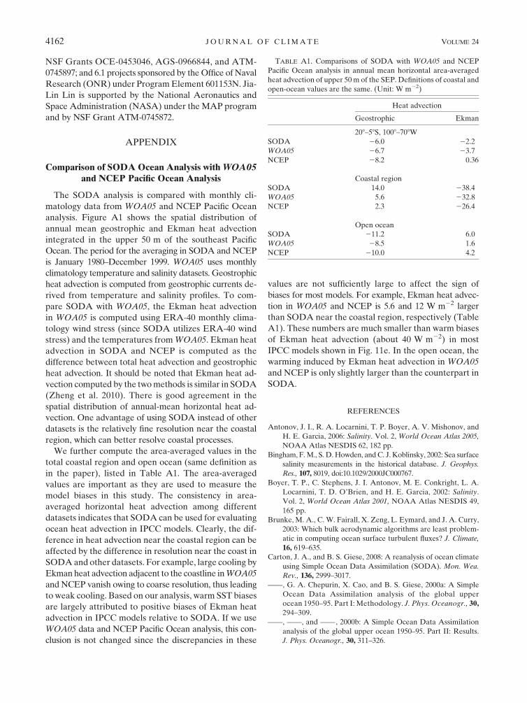
FIG. A1. Comparisons of the spatial distribution of annual mean geostrophic and Ekman heat advection integrated in

the upper 50 m of the southeast Pacific Ocean between SODA and WOA05 as well as NCEP Pacific Ocean analysis.


NSF Grants OCE-0453046, AGS-0966844, and ATM-

0745897; and 6.1 projects sponsored by the Office of Naval

Research (ONR) under Program Element 601153N. Jia-

Lin Lin is supported by the National Aeronautics and

Space Administration (NASA) under the MAP program

and by NSF Grant ATM-0745872.

APPENDIX

Comparison of SODA Ocean Analysis with WOA05and NCEP Pacific Ocean Analysis

The SODA analysis is compared with monthly cli-

matology data from WOA05 and NCEP Pacific Ocean

analysis. Figure A1 shows the spatial distribution of

annual mean geostrophic and Ekman heat advection

integrated in the upper 50 m of the southeast Pacific

Ocean. The period for the averaging in SODA and NCEP

is January 1980–December 1999. WOA05 uses monthly

climatology temperature and salinity datasets. Geostrophic

heat advection is computed from geostrophic currents de-

rived from temperature and salinity profiles. To com-

pare SODA with WOA05, the Ekman heat advection

in WOA05 is computed using ERA-40 monthly clima-

tology wind stress (since SODA utilizes ERA-40 wind

stress) and the temperatures from WOA05. Ekman heat

advection in SODA and NCEP is computed as the

difference between total heat advection and geostrophic

heat advection. It should be noted that Ekman heat ad-

vection computed by the two methods is similar in SODA

(Zheng et al. 2010). There is good agreement in the

spatial distribution of annual-mean horizontal heat ad-

vection. One advantage of using SODA instead of other

datasets is the relatively fine resolution near the coastal

region, which can better resolve coastal processes.

We further compute the area-averaged values in the

total coastal region and open ocean (same definition as

in the paper), listed in Table A1. The area-averaged

values are important as they are used to measure the

model biases in this study. The consistency in area-

averaged horizontal heat advection among different

datasets indicates that SODA can be used for evaluating

ocean heat advection in IPCC models. Clearly, the dif-

ference in heat advection near the coastal region can be

affected by the difference in resolution near the coast in

SODA and other datasets. For example, large cooling by

Ekman heat advection adjacent to the coastline in WOA05

and NCEP vanish owing to coarse resolution, thus leading

to weak cooling. Based on our analysis, warm SST biases

are largely attributed to positive biases of Ekman heat

advection in IPCC models relative to SODA. If we use

WOA05 data and NCEP Pacific Ocean analysis, this con-

clusion is not changed since the discrepancies in these

values are not sufficiently large to affect the sign of

biases for most models. For example, Ekman heat advec-

tion in WOA05 and NCEP is 5.6 and 12 W m22 larger

than SODA near the coastal region, respectively (Table

A1). These numbers are much smaller than warm biases

of Ekman heat advection (about 40 W m22) in most

IPCC models shown in Fig. 11e. In the open ocean, the

warming induced by Ekman heat advection in WOA05

and NCEP is only slightly larger than the counterpart in

SODA.

REFERENCES

Antonov, J. I., R. A. Locarnini, T. P. Boyer, A. V. Mishonov, and

H. E. Garcia, 2006: Salinity. Vol. 2, World Ocean Atlas 2005,

NOAA Atlas NESDIS 62, 182 pp.

Bingham, F. M., S. D. Howden, and C. J. Koblinsky, 2002: Sea surface

salinity measurements in the historical database. J. Geophys.

Res., 107, 8019, doi:10.1029/2000JC000767.

Boyer, T. P., C. Stephens, J. I. Antonov, M. E. Conkright, L. A.

Locarnini, T. D. O’Brien, and H. E. Garcia, 2002: Salinity.

Vol. 2, World Ocean Atlas 2001, NOAA Atlas NESDIS 49,

165 pp.

Brunke, M. A., C. W. Fairall, X. Zeng, L. Eymard, and J. A. Curry,

2003: Which bulk aerodynamic algorithms are least problem-

atic in computing ocean surface turbulent fluxes? J. Climate,

16, 619–635.

Carton, J. A., and B. S. Giese, 2008: A reanalysis of ocean climate

using Simple Ocean Data Assimilation (SODA). Mon. Wea.

Rev., 136, 2999–3017.

——, G. A. Chepurin, X. Cao, and B. S. Giese, 2000a: A Simple

Ocean Data Assimilation analysis of the global upper

ocean 1950–95. Part I: Methodology. J. Phys. Oceanogr., 30,

294–309.

——, ——, and ——, 2000b: A Simple Ocean Data Assimilation

analysis of the global upper ocean 1950–95. Part II: Results.

J. Phys. Oceanogr., 30, 311–326.

TABLE A1. Comparisons of SODA with WOA05 and NCEP

Pacific Ocean analysis in annual mean horizontal area-averaged

heat advection of upper 50 m of the SEP. Definitions of coastal and

open-ocean values are the same. (Unit: W m22)

Heat advection

Geostrophic Ekman

208–58S, 1008–708W

SODA 26.0 22.2

WOA05 26.7 23.7

NCEP 28.2 0.36

Coastal region

SODA 14.0 238.4

WOA05 5.6 232.8

NCEP 2.3 226.4

Open ocean

SODA 211.2 6.0

WOA05 28.5 1.6

NCEP 210.0 4.2


Chou, S.-H., E. Nelkin, J. Ardizzone, R. M. Atlas, and C.-L. Shie,

2003: Surface turbulent heat and momentum fluxes over

global oceans based on the Goddard satellite retrievals, ver-

sion 2 (GSSTF2). J. Climate, 16, 3256–3273.

——, ——, ——, and ——, 2004: A comparison of latent heat fluxes

over global oceans for four flux products. J. Climate, 17, 3973–

3989.

Colbo, K., and R. Weller, 2007: The variability and heat budget of

the upper ocean under the Chile-Peru stratus. J. Mar. Res., 65,

607–637.

de Szoeke, S. P., and X.-P. Xie, 2008: The tropical eastern Pacific

seasonal cycle: Assessment of errors and mechanisms in IPCC

AR4 coupled ocean–atmosphere general circulation models.

J. Climate, 21, 2573–2590.

——, C. W. Fairall, D. E. Wolfe, L. Bariteau, and P. Zuidema, 2010:

Surface flux observations on the southeastern tropical Pacific

Ocean and attribution of SST errors in coupled ocean–

atmosphere models. J. Climate, 23, 4152–4174.

Diaz, H., C. Folland, T. Manabe, D. Parker, R. Reynolds, and

S. Woodruff, 2002: Workshop on advances in the use of his-

torical marine climate data. WMO Bull., 51, 377–380.

Fairall, C. W., E. F. Bradley, J. E. Hare, A. A. Grachev, and J. B.

Edson, 2003: Bulk parameterization of air–sea fluxes: Updates

and verification for the COARE algorithm. J. Climate, 16,

571–591.

Garreaud, R. D., and R. C. Munoz, 2005: The low-level jet off the

west coast of subtropical South America: Structure and vari-

ability. Mon. Wea. Rev., 133, 2246–2261.

Gent, P. R., S. G. Yeager, R. B. Neale, S. Levis, and D. A. Bailey,

2009: Improvements in a half degree atmosphere/land version

of the CCSM. Climate Dyn., 34, 819–833, doi:10.1007/s00382-

009-0614-8.

Gordon, C. T., A. Rosati, and R. Gudgel, 2000: Tropical sensitivity

of a coupled model to specified ISCCP low clouds. J. Climate,

13, 2239–2260.

Jones, P. W., 1999: First- and second-order conservative remapping

schemes for grids in spherical coordinates. Mon. Wea. Rev.,

127, 2204–2210.

Kalnay, E., and Coauthors, 1996: The NCEP/NCAR 40-Year Re-

analysis Project. Bull. Amer. Meteor. Soc., 77, 437–471.

Kanamitsu, M., W. Ebisuzaki, J. Woollen, S.-K. Yang, J. J.

Hnilo, M. Fiorino, and G. L. Potter, 2002: NCEP–DOE

AMIP-II Reanalysis (R-2). Bull. Amer. Meteor. Soc., 83,

1631–1643.

Kiehl, J. T., and P. R. Gent, 2004: The Community Climate System

Model, version 2. J. Climate, 17, 3666–3682.

Kubota, M., A. Kano, H. Muramatsu, and H. Tomita, 2003: In-

tercomparison of various surface heat flux fields. J. Climate,

16, 670–678.

Large, W. G., and G. Danabasoglu, 2006: Attribution and im-

pacts of upper-ocean biases in CCSM3. J. Climate, 19, 2325–

2346.

——, J. C. McWilliams, and S. C. Doney, 1994: Oceanic vertical

mixing: Review and model with a nonlocal boundary layer

parameterization. Rev. Geophys., 32, 363–403.

Lin, J.-L., 2007: The double-ITCZ problem in IPCC AR4 coupled

GCMs: Ocean–atmosphere feedback analysis. J. Climate, 20,

4497–4525.

Locarnini, R. A., A. V. Mishonov, J. I. Antonov, T. P. Boyer, and

H. E. Garcia, 2006: Temperature. Vol. 1, World Ocean Atlas

2005, NOAA Atlas NESDIS 61, 182 pp.

Ma, C.-C., C. R. Mechoso, A. W. Robertson, and A. Arakawa,

1996: Peruvian stratus clouds and the tropical Pacific circulation:

A coupled ocean–atmosphere GCM study. J. Climate, 9, 1635–

1645.

McAvaney, B., and Coauthors, 2001: Model evaluation. Climate

Change 2001: The Scientific Basis, J. T. Houghton et al., Eds.,

Cambridge University Press, 471–523.

McWilliams, J. C., and F. Colas, 2010: Climate heat balance off

western South America: Regional oceanic circulation and

eddies. CLIVAR Exchanges, No. 53, International CLIVAR

Project Office, Southampton, United Kingdom, 14–16.

Mechoso, C. R., and Coauthors, 1995: The seasonal cycle over the

tropical Pacific in coupled ocean–atmosphere general circu-

lation models. Mon. Wea. Rev., 123, 2825–2838.

Miller, R. L., 1997: Tropical thermostats and low cloud cover.

J. Climate, 10, 409–440.

Rossow, W. B., A. W. Walker, D. E. Beuschel, and M. D. Roiter,

1996: International Satellite Cloud Climatology Project

(ISCCP) documentation of new cloud datasets. WMO Tech.

Doc. 737, 115 pp.

Shinoda, T., and J. L. Lin, 2009: Interannual variability of the upper

ocean in the southeast Pacific stratus cloud region. J. Climate,

22, 5072–5088.

Simmons, A. J., and J. K. Gibson, 2002: The ERA-40 Project Plan.

ECMWF ERA-40 Project Report Series 1, 63 pp.

Smith, R. D., J. K. Dukowicz, and R. C. Malone, 1992: Parallel

ocean general circulation modeling. Physica D, 60, 38–61.

Stephens, C., J. I. Antonov, T. P. Boyer, M. E. Conkright, R. A.

Locarnini, T. D. O’Brien, and H. E. Garcia, 2002: Tempera-

ture. Vol. 1, World Ocean Atlas 2001, NOAA Atlas NESDIS

49, 169 pp.

Straneo, F., C. F. Moffat, R. A. Weller, and J. T. Farrar, 2010:

Eddies in the southeast Pacific and their influence on the upper

ocean. Extended Abstracts, 2010 Fall Meeting, San Francisco,

CA, Amer. Geophys. Union, A54B-02. [Available online at

http://adsabs.harvard.edu/abs/2010AGUFM.A54B..02S.]

Toniazzo, T., C. R. Mechoso, L. C. Shaffrey, and J. M. Slingo, 2010:

Upper-ocean heat budget and ocean eddy transport in the

south-east Pacific in a high-resolution coupled model. Climate

Dyn., 35, 1309–1329, doi:10.1007/s00382-009-0703-8.

Uppala, S. M., and Coauthors, 2005: The ERA-40 Re-Analysis.

Quart. J. Roy. Meteor. Soc., 131, 2961–3012.

Wittenberg, A. T., A. Rosati, N.-C. Lau, and J. J. Ploshay,

2006: GFDL’s CM2 global coupled climate models. Part

III: Tropical Pacific climate and ENSO. J. Climate, 19,

698–722.

Wood, R., C. Bretherton, B. Huebert, C. R. Mechoso, and

R. Weller, 2007: The VAMOS Ocean-Cloud-Atmosphere-

Land Study (VOCALS): Improving understanding, model

simulations, and prediction of the southeast Pacific climate

system. Post-VOCALS-Rex Rep., 17 pp. [Available online at

http://www.atmos.ucla.edu/~mechoso/Intro_Final.pdf.]

Xie, S.-P., 2004: The shape of continents, air-sea interaction, and

the rising branch of the Hadley circulation. The Hadley Circu-

lation: Past, Present and Future, H. F. Diaz and R. S. Bradley,

Eds., Kluwer Academic Publishers, 121–152.

Yu, L., and R. A. Weller, 2007: Objectively analyzed air–sea heat

fluxes for the global ice-free oceans (1981–2005). Bull. Amer.

Meteor. Soc., 88, 527–539.

——, X. Jin, and R. A. Weller, 2008: Multidecade global flux da-

tasets from the objectively analyzed air-sea fluxes (OAFlux)

project: Latent and sensible heat fluxes, ocean evaporation,

and related surface meteorological variables. Woods Hole

Oceanographic Institution OAFlux Project Tech. Rep. OA-

2008-01, 64 pp.


Zappa, C. J., J. T. Farrar, R. A. Weller, S. P. Bigorre, L. St Laurent,

F. Straneo, and C. F. Moffat, cited 2010: Upper-ocean turbu-

lence beneath the stratus cloud deck of the southeast Pacific.

[Available online at http://adsabs.harvard.edu/abs/2010AGUFM.

A51A0047Z.]

Zhang, Y., W. B. Rossow, A. A. Lacis, V. Oinas, and M. I.

Mishchenko, 2004: Calculation of radiative fluxes from the

surface to top of atmosphere based on ISCCP and other

global data sets: Refinements of the radiative transfer model

and the input data. J. Geophys. Res., 109, D19105, doi:10.1029/

2003JD004457.

Zheng, Y., and B. S. Giese, 2009: Ocean heat transport in Simple

Ocean Data Assimilation: Structure and mechanisms. J. Geo-

phys. Res., 114, C11009, doi:10.1029/2008JC005190.

——, T. Shinoda, G. N. Kiladis, J.-L. Lin, E. J. Metzger, H. E.

Hurlburt, and B. S. Giese, 2010: Upper-ocean processes under

the stratus cloud deck in the southeast Pacific Ocean. J. Phys.

Oceanogr., 40, 103–120.


Sea Surface Temperature Biases under the Stratus Cloud ...

Documents

Transcript of Sea Surface Temperature Biases under the Stratus Cloud ...