Sea Clutter Reduction and Target Enhancement by Neural Networks in a Marine Radar System

Sensors 2009, 9, 1913-1936; doi:10.3390/s90301913

OPEN ACCESS

sensorsISSN 1424-8220

www.mdpi.com/journal/sensors

Article

Sea Clutter Reduction and Target Enhancement by NeuralNetworks in a Marine Radar SystemRaul Vicen-Bueno ?, Ruben Carrasco-Alvarez, Manuel Rosa-Zurera and Jose Carlos Nieto-Borge

Signal Theory and Communications Department, Superior Politechnic School, University of Alcala,Alcala de Henares, 28805, Madrid, Spain

E-mails: [email protected]; [email protected]; [email protected]; [email protected]

? Author to whom correspondence should be addressed:E-mail: [email protected], Tel.: +34 91 885 6700, Fax: +34 91 885 6699, URL: http://ssp.uah.es/∼raul

Received: 18 December 2008; in revised form: 16 February 2009 / Accepted: 11 March 2009 /Published: 16 March 2009

Abstract: The presence of sea clutter in marine radar signals is sometimes not desired. So,efficient radar signal processing techniques are needed to reduce it. In this way, nonlinearsignal processing techniques based on neural networks (NNs) are used in the proposed clutterreduction system. The developed experiments show promising results characterized by differ-ent subjective (visual analysis of the processed radar images) and objective (clutter reduction,target enhancement and signal-to-clutter ratio improvement) criteria. Moreover, a deep studyof the NN structure is done, where the low computational cost and the high processing speedof the proposed NN structure are emphasized.

Keywords: Neural Networks; Non-linear Signal Processing; Radar; Remote Sensing; ClutterReduction; Target Enhancement; SCR Improvement.

1. Introduction

The measurement of radar backscatter from an ocean surface, usually referred to as sea clutter, playsan important role in ocean surveillance and remote sensing. In particular, two different points of viewmay be identified depending on the application. From the first one, sea clutter contains useful informationabout the ocean surface and the characterization of sea clutter becomes the focal point of the study. From

Sensors 2009, 9 1914

the second one, if the primary objective is the detection of targets, such as ships and/or boats, then, thepresence of sea clutter is viewed as a source of interference to be suppressed. The studies presented inthis paper are focused on the last case, where the suppression of sea clutter signals and the enhancementof signals related to ship/s play an important role.

The clutter reduction system explained in this paper is proposed to be used in conventional radarsystems. These general purpose systems measure only the intensity of the returned electromagnetic echo,where no phase information is given (non-coherent/incoherent radar systems). These kind of systems arecommonly used, for instance, in marine traffic control centers. Moreover, the proposed clutter reductionsystem, among other final applications, can be used to improve the information managed by automaticidentification systems (AISs) [1], such as the accurate positioning and tracking of surrounding ships byradar measurements, which lets improve the safety of marine navigation.

Previous experiments of other researchers using different clutter reduction techniques denote thatpromising results can be achieved. In this way, in [2] a large number of clutter reduction methodsapplied to different problems are analyzed. This work classifies them both in terms of how they deal withclutter reduction and more importantly, in terms of the benefits and losses depending on the applicationwhere they are applied to. Moreover, the same authors of the previous work analyze in [3] an automaticprocedure to reduce the level of clutter signals in parallel coordinates plots applied to different problems.The previous referenced work is important in our studies because they work with the same coordinatesas the ones used during our experiments.

On the other hand, and focusing on the remote sensing technology we work with in this paper, dif-ferent approaches have been satisfactorily used. These approaches can be divided, among others, inthree categories: conventional methods based on statistical models, image processing-based methodsand methods based on neural networks (NNs), which are relatively novel. Before continuing, it is impor-tant to note that due to the speed of movement (doppler effect) of the targets (ships) and the sea clutter(waves) considered in our studies, linear filtering cannot be applied (overlapping of the target and clutterspectra). Moreover, the dynamic of the sea clutter is intrinsically nonlinear. So, due to both reasons, anonlinear signal processing is needed.

In conventional methods, an statistical model is supposed a priori (Weibull-distributed clutter, k-distributed clutter, etc.), which involves the main statistical effects of the clutter. In this way, an approachto reduce ground clutter based on statistical signal processing techniques is proposed in [4]. This ap-proach is based on the use of a simple parametric model, what limits the application of these techniquesto other kind of clutters, such as sea clutter. Other approaches, based on statistical signal processing,such as principal component analysis (PCA) [5] and independent component analysis (ICA) [6], havebeen successfully applied to ground clutter reduction. Moreover, other statistical-based techniques, suchas the estimation of target and clutter signal parameters by the use of the likelihood ratio test [7], areused to reduce the level of clutter in surface penetrating impulse radars.

In image processing-based methods, several ones could be cited, but we focus on commonly usedmethods based on transform domains. One of them is based on the reduction of clutter in radar imagesby a translation invariant wavelet packet decomposition [8, 9]. Other techniques use the information con-tained in temporal radar image sequences [10], what makes the system work slow (high computationalcost and memory requirements) or with some delay in the presentation of information to the user.

Sensors 2009, 9 1915

The last category is based on NNs, which is the aim of our proposal. In these methods, the a prioriknowledge of the statistical distributions of the target and clutter and their parameters is not necessary,as occur with the conventional (classical) methods. During the NN training, the NN is able to learn thestatistical behavior of the training data, what make it a suitable method to infer the statistical distributionof the data (target and clutter) and its parameters. So, for instance, the use of NNs, such as the onesbased on radial basis functions (RBFs), denotes the suitable applicability of these techniques to radartarget detection based on clutter modeling [11]. Moreover, this kind of NNs are successfully used infinal radar applications, such as automatic target detection in clutter by clutter modelling [12], which canbe considered as a future application of the clutter reduction system proposed. On the other hand, anAdaptive-Network-based Fuzzy Inference System (ANFIS) architecture has been successfully appliedin [13] to classify different kind of weather radar clutters. So, as a NN can be an inner element of anANFIS architecture, this architecture can be used in the future to improve the clutter reduction achievedby NN-based systems.

After observing that clutter reduction (in general) is successfully applied in different kinds of radarsystems (ground, sea, etc.), we now focus on the particular topic presented in this paper, i.e., the reductionof sea clutter in radar images. Moreover, because of the promising results achieved with NNs in previousstudies where clutter modeling was used [11, 12], the clutter reduction system proposed in our paperis also based on NNs. But considering that these works [11, 12] are based on RBF-NNs, the proposedsystem is focused on a different NN category, the multilayer perceptron (MLP), where different activationfunctions to the RBF-NNs, different NN training algorithm (supervised training) and a different way toselect the input data are used. The proposed NN-based sea clutter reduction system also defers from theprevious ones based on RBF-NNs because it is proposed as a nonlinear filter instead of a clutter modelingsystem used to detect radar targets. The proposed system presents several advantages. First, it can beused in commonly used radar systems (incoherent radar systems). Second, due to the used NNs (MLPs)are able to implement nonlinear transfer functions, they are able to solve the problem of separation ofclutter and target signals in order to reduce the level of (sea) clutter and enhance the level of target (ship).Third, neither the knowledge of the statistical distribution of the target and clutter nor their parametersare not necessary a priori, as in the conventional/classical methods. In this case, just only a set of radarimages and their desired outputs are needed to train the NN. And fourth, the proposed method filters outthe sea clutter pixel by pixel in each image and it doesn’t require a sequence of radar images, as severalimage processing-based techniques do. This advantage makes it faster processing radar images.

In order to cover the explanation of the proposed system, the paper is organized in five sections,including the current one. Section 2. describes the platform used to get the radar measurements, whichwas successfully used in other research works [10]. The structure and design of the proposed NN-based clutter reduction system is explained in Section 3. The results obtained with the proposed systemare presented in Section 4., where a system dimensionality study is carried out and a subjective and anobjective analysis of the results is done. So, the results analysis from the subjective point of view focuseson the visual analysis and the subjective interpretation of the radar images at the output of the proposedsystem. Whereas, the analysis of the results from the objective point of view focuses on two kind ofestimations. First, the error between the desired and the obtained radar image outputs is estimated. Andsecond, certain parameters of radar signals are estimated, such as the relationship between the clutter and

Sensors 2009, 9 1916

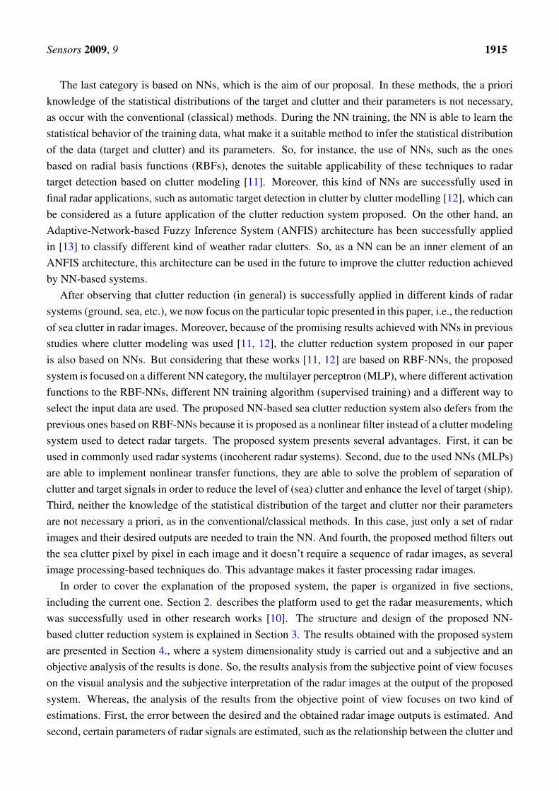
Figure 1. FINO 1 Emplacement in the North Sea and Measuring and Monitoring MarineSystem Location

Research platform location:Borkum Riff(45 km north of Borkum island)

N 54° 0.86' E 6° 35.26'

North Sea

Measuring and Monitoring Marine System

! !! !!

the target average powers, which let us to estimate the signal-to-clutter ratio (SCR). This performanceevaluation let us to estimate the performance improvement achieved by the proposed system. Finally, themain conclusions and contributions of the proposed system are exposed in Section 5., including severalaspects that could be improved in the future.

2. Measuring and Monitoring Marine System

The radar measurements considered in our experiments were acquired in the FINO 1 (Forschungsplat-tformen in Nord-und Ostsee) German research platform located at the German basin of the North Sea(see Figure 1). In this platform, an incoherent radar system is available and a WaMoS II system [14]is installed, which compose the measuring and monitoring marine system used during the experiments(Figure 1). The WaMoS II system is an operational Wave Monitoring System developed by the Germanresearch institute GKSS and commercialized by OceanWaveS GmbH. This system acquires every fiveminutes a temporal sequence of 32 consecutive radar images. The intensity of each radar image cellis coded without sign and 1 byte (8 bits), what sets a dynamic range of [0 − 255]. The sampling time(Ts) of this temporal sequence of radar images corresponds to the antenna rotation period. The spatialresolutions (Rx and Ry) of each image depends on the azimuthal and range resolutions of the radarsystem.

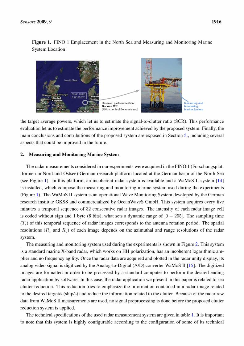
The measuring and monitoring system used during the experiments is shown in Figure 2. This systemis a standard marine X-band radar, which works on HH polarization, has an incoherent logarithmic am-plier and no frequency agility. Once the radar data are acquired and plotted in the radar unity display, itsanalog video signal is digitized by the Analog-to-Digital (A/D) converter WaMoS II [15]. The digitizedimages are formatted in order to be processed by a standard computer to perform the desired endingradar application by software. In this case, the radar application we present in this paper is related to seaclutter reduction. This reduction tries to emphasize the information contained in a radar image relatedto the desired target/s (ship/s) and reduce the information related to the clutter. Because of the radar rawdata from WaMoS II measurements are used, no signal preprocessing is done before the proposed clutterreduction system is applied.

The technical specifications of the used radar measurement system are given in table 1. It is importantto note that this system is highly configurable according to the configuration of some of its technical

Sensors 2009, 9 1917

Figure 2. Measuring and Monitoring Marine System

2. ADQUISITION OF OCEAN WAVE DATA BY

USING MARINE RADARS

It is known that, under various conditions, signatures

of the sea surface are visible in marine X-Band radar images

[1, 2]. These signatures are known as sea clutter, which is

undesirable for navigation purposes. Therefore, the sea clut-

ter is generally suppressed by filtering algorithms. Sea clut-

ter is caused by the backscatter of the transmitted electro-

magnetic waves from the short sea surface ripples in the

range of the electromagnetic wavelength (e.g. ~3 cm).

Hence, longer waves like swell and wind sea become visible

as they modulate the backscatter signal. Figure 1 shows a

digitized sea clutter image where a wave field is imaged by

a marine radar.

Since standard X-Band marine radar systems allow to

scan the sea surface with high temporal and spatial resolu-

tion, they are able to monitor the sea surface in time and

space. Hence, the combination of the temporal and special

wave information permits to obtain unambiguous directional

wave spectra. As marine radar imagery cover an area of the

sea surface it allows to observe also spatial variation in the

wave field. Furthermore, the use of marine radars allows the

detection of wave field features on moving ships, as well as

on and offshore platforms. The next section describes the

measuring system used in the work.

2.1 Description of the measuring system

In the past different marine radar based systems to

measure the sea state have been developed. This paper uses

on one of these devices, the German system WaMoS II

(Wave Monitoring System).WaMoS II is a high-speed video

digitizing and storage device that can be interfaced to any

conventional navigational X-Band radar and a software

package [1]. The software controls the radar and data stor-

age. In addition, the WaMoS II software carries out the

wave analysis and displays the results. A typical WaMoS II

wave measurement consists of the acquisition of radar im-

age sequences and its wave analysis results. Figure 2 shows

a scheme of a typical WaMoS II installation. The standard

WaMoS II analysis uses a sequence of 32 radar images.

Waves in the range of 0.025 Hz to 0.35 Hz can be detected.

The actual range, resolution and accuracy can vary for each

WaMoS II installation, depending on the used radar and set-

up geometry.

Figure 2 – Scheme showing a typical installation of the ocean

wave measuring system used in this work.

3. ANALYSIS OF SEA STATE PARAMETERS

3.1 Estimation of the image spectrum

To analyze the spatial and temporal structure of the

imaged wave field, the first step consist of measuring a tem-

poral sequence of sea clutter images. Hence, applying a

three-dimensional Fourier decomposition, the so-called im-

age spectrum I(k, !) is estimated. k = (kx, ky) is the wave

number vector and ! is the angular frequency of the sea

clutter time series. Figure 3 illustrates a frequency-wave

number transect of the three-dimensional image spectrum

obtained from a sea clutter time series measured in the re-

search platform of FINO 1 in the North Sea. Figure 3 shows

that I(k, !) contains different contributions located at differ-

ent regions within the spectral domain (k, !). The region of

higher spectral intensity corresponds to the dispersion rela-

tion, !(k), of linear ocean waves. This dispersion relation

corresponds to the following expression

! = gk tanh(kd) + k "U , (1)

where, g is the gravity acceleration, d is the water depth, k is

the modulus of k, and U=(Ux, Uy) is the so-called current of

encounter. U causes a Doppler shift in frequency due to the

relative motion between the radar antenna and the wave field.

For measurements carried out at a fixed platform rather that a

moving ship, U is caused by the existence of an ocean cur-

rent [1, 2, 3].


USING MARINE RADARS












a marine radar.





























up geometry.




















! = gk tanh(kd) + k "U , (1)







rent [1, 2, 3].


USING MARINE RADARS












a marine radar.





























up geometry.




















! = gk tanh(kd) + k "U , (1)







rent [1, 2, 3].


USING MARINE RADARS












a marine radar.





























up geometry.




















! = gk tanh(kd) + k "U , (1)







rent [1, 2, 3].

Radar Environment

X-Band MarineRadar Antenna

TxRx

Radar Unity(Transmitter and Receiver)

Radar Unity(Display)

Data Storage and Processing

A/D Converter(WaMos II)

Rx Rx Rx

Table 1. Radar Measurement System Characteristics in Transmission and Reception

Radar System Frequency (X-band) 10.0 GHz

Antenna Rotation Speed 50 rpm

Antenna Polarization H and H

Pulse Repetition Frequency (PRF) 1000 Hz

Radar Pulse Width 80 ns

Distance Range (Coverage) 200− 2150 m

Range Resolution 7.5 m

Azimuthal Range (Coverage) 0 - 360 ◦

Azimuthal Resolution 0.28 ◦

parameters. Moreover, the inhibition of several scan sectors during the radar measurements is possible,as can be observed in the radar images presented in Section 4.

3. NN-based Clutter Reduction System

NNs, and exactly MLPs, are able to learn the statistical distribution of the input data to give thedesired output from the input-output data relationship during a training process. In this way, consideringa supervised training, where the desired outputs are known, the input data are presented to the NN andtheir corresponding outputs are obtained. According to the obtained output, the NN is able to adapt itstransfer function during the training process (design stage) in order to minimize a certain error between

Sensors 2009, 9 1918

the desired and obtained outputs. Once the NN is trained (design stage), it is tested (test stage) in order toanalyze its behavior with other input data, which are different of the data used during the design stage. Itis important to note that in the test stage is not mandatory to know which are the desired outputs as occurin the design stage. So, due to the above mentioned capabilities of learning from the input-output datarelationship of an MLP during a supervised training, an MLP is used to learn the statistical behavior ofthe clutter and targets (ships) signals contained in radar images. The different kinds of clutter and targetare exposed in the presentation of the radar image database used during the experiments (see subsection4.1.). This learning lets the MLP maximizes the separation between target and clutter information at itsoutput. This separation is evaluated in the results section as the SCR improvement, where, in this case,the desired output radar images are known in order to give an objective performance of the system. Onthe other hand, the system, once designed, can work with this knowledge of the desired output, becausea subjective analysis can be also done, as it is shown in the results section too.

Once the basis of the proposed NN-based clutter reduction system is explained, several aspects aredescribed in the next subsections. These aspects focus on how the radar image at the output of thesystem is achieved, how the output error is estimated, what kind of MLP training algorithm is used, howto design and test the system, what kind of evaluation of the system performance is done and which arethe steps followed to study the dimensionality of the NN.

3.1. System Processing: Output Radar Image Achievement

Independently of the MLP stage (design or test), the way the NN-based clutter reduction systemprocesses the data of the radar measurements included in the input radar image (I) to obtain the processedoutput radar image (O) is summarized in Figure 3. This figure shows how the MLP output y(o) is obtainedfor a cell under test (CUT). Moreover, it is also shown how this output is assigned to the correspondingcell of the output radar image (or,c), which is established by the r-th row and c-th column of the CUT inthe input radar image. Note that only one MLP output is selected because the objective is processing eachvalid cell of the input radar image and obtaining an output radar image of the same size as the input one.In our case of study, a total of 5 radar return measurements for different positions (range and azimuth) areconsidered, where they are selected from horizontal radar image raw data. Note that due to the circularsymmetry of the coverage and the freedom of waves movement and ships navigation (they can movein whatever direction), a vertical orientation could be selected obtaining similar system performances.Other choice could be use a different shape of selecting the surrounding data of the CUT, what could bestudied in the future. Moreover, note that from these 5 selected measurements of I for each CUT, thecentral element (ir,c) corresponds to the CUT, and the others correspond to surrounding measurements,where a symmetric distribution of the selected data is done. This symmetric selection is done in orderto have the same quantity of information from both sides. This number of measurements (empiricallyobtained) is selected as a trade-off between the system performance, the MLP computational complexityand the size of the targets (ships) under study. Note that 5 cells with a range resolution of 7.5 m (see table1) involve a distance of 37.5 m, which is the minimum range necessary to englobe the beam of all theships under study (see table 2 of subsection 4.1.) in case they are perpendicularly placed with respect tothe orientation of the selection of input data. As can be observed, the MLP architecture depends on thecharacteristics of the target to be enhanced. On the other hand, following the nomenclature established

Sensors 2009, 9 1919

Figure 3. NN-based clutter reduction system

Ra

ng

e (m

)

Range (m)

!2

00

0!

15

00

!1

00

0!

50

00

50

01

00

01

50

02

00

0

!2

00

0

!1

50

0

!1

00

0

!5

00 0

50

0

10

00

15

00

20

00

Min

imu

m

Lo

w

Me

diu

m

Hig

h

Ma

xim

um

NN-based ClutterReduction System

MultiLayerPerceptron(MLP)

Inpu

t Vec

tor (

x)Co

mpo

sitio

n

Range (m

)

Range (m)

!2

00

0!

15

00

!1

00

0!

50

00

50

01

00

01

50

02

00

0

!2

00

0

!1

50

0

!1

00

0

!5

00 0

50

0

10

00

15

00

20

00

Min

imu

m

Lo

w

Me

diu

m

Hig

h

Ma

xim

um

Ra

ng

e (m

)

Range (m)

!2000

!1500

!1000

!500

0500

1000

1500

2000

!2000

!1500

!1000

!500 0

500

1000

1500

2000

Min

imum

Low

Mediu

m

Hig

h

Maxim

um

Ra

ng

e (m

)

Range (m)

!2

00

0!

15

00

!1

00

0!

50

00

50

01

00

01

50

02

00

0

!2

00

0

!1

50

0

!1

00

0

!5

00 0

50

0

10

00

15

00

20

00

Min

imu

m

Lo

w

Me

diu

m

Hig

h

Ma

xim

um

Input Radar Image (I:Zoom of a segment

Radar Image at the Input (I) of the NN-based Clutter

Reduction System

ir,c-1 ir,c

x4 x3

CUT

or,c

Output Radar Image (O):Zoom of a segment

ir,c+1

x2

ir,c+2

x1

ir,c-2

x5

CUT

Utan( )bH(h)

y(o)

Utan( )b1(h)Utan( )b2

(h)

W1,1(h)W1,2

(h)W1,H(h)

W5,1(h)W5,2

(h)W5,H(h)

... ...

... ...

... ... ...

Ulog( )b(o)

wH(o) w2

(o) w1(o)

Hidd

en

Neur

on H

Hidd

en

Neur

on 2

Hidd

en

Neur

on 1

Out

put

Neur

on

Radar Image at the Output (O) of the NN-based Clutter

Reduction System

y2(h) y1

(h)yH(h)

/255 /255 /255/255 /255

x255

in Figure 3 and taking into account the dynamic range of the input data (8 bits: dynamic range of[0 − 255]), the processed output (or,c = round(y(o) · 255)) for a given CUT and its surrounding cells,which are contained in the input vector x = [x1, x2, x3, x4, x5] = [ir,c−2, ir,c−1, ir,c, ir,c+1, ir,c+2]/255, isgiven by:

y(o) = fNN(x) (1)

where fNN(·) denotes the transfer function implemented by the NN. Note that the NN inputs (x) arenormalized to a range [0 − 1]. Moreover, due to the activation function selected for the NN outputneuron, its output (y(o)) is limited to the range [0− 1], as shown below.

Once the way the radar measurements selection to the MLP input for each CUT is exposed and jus-tified, the MLP output computation is presented. In our case of study, we have considered an MLPcomposed of 5 inputs, H hidden neurons and 1 output neuron, i.e., a structure 5/H/1 with two lay-ers (one hidden layer and the output layer), where H is a parameter under study in our experiments.Moreover, due to inner property of the unknown nonlinear dynamic of the sea clutter during time andthe possible overlapping of the moving target and clutter spectra (doppler effect), a nonlinear system isneeded because linear solutions are not suitable for this purpose. In this way, this nonlinear function canbe achieved by the used NN and its implemented transfer function (fNN(·)).

The way to obtain the MLP output is presented below in the same way the MLP processes the data,

Sensors 2009, 9 1920

i.e., first the hidden neuron outputs are achieved and finally the MLP output is obtained. In this way,considering v(h)

j is the overall weighted input of the j-th hidden neuron, which is obtained by eq. (2),the j-th hidden neuron output (y(h)

j ) can be computed by eq. (3), where a (nonlinear) hyperbolic tangentactivation function (ψtan(·)) [16] is used.

v(h)j =

(5∑

i=1

xi · w(h)i,j

)+ b

(h)j (2)

y(h)j = ψtan

(v

(h)j

)=

sinh(v(h)j )

cosh(v(h)j )

=ev

(h)j − e−v

(h)j

ev(h)j + e−v

(h)j

(3)

Note that the element w(h)i,j denotes the MLP synaptic weight that connects the i-th input (xi) with the

j-th hidden neuron (see Figure 3). So, W(h) is the matrix that contains the synaptic weights that connectthe MLP inputs with the MLP hidden neurons. Moreover, b(h)

j denotes the bias of the j-th hidden neuron,where the row vector b(h) contains all the hidden neuron biases. For our case of study, W(h) contains atotal of [5xH] synaptic weights and b(h) contains a total of [1xH] bias weights.

Following the MLP computation procedure, and considering v(o) is the overall weighted input of theoutput neuron, which is obtained by eq. (4), the neuron output (y(o)) can be computed by eq. (5). In thiscase, this neuron uses a (nonlinear) logistic activation function (ψlog(·)) [16] because of the need that theMLP output is limited between 0 and 1.

v(o) =

H∑j=1

y(h)j · w(o)

j

+ b(o) (4)

y(o) = ψlog

(v(o)

)=

1

1 + ev(o) (5)

Note that the element w(o)j denotes the MLP synaptic weight that connects the output of the j-th hidden

neuron (y(h)j ) with the output neuron (see Figure 3), where the column vector w(o) contains all these

weights. Moreover, b(o) denotes the bias of the output neuron. For our case of study, w(o) contains a totalof [Hx1] synaptic weights and b(o) contains a total of [1x1] bias weight.

Summarizing, the NN-based clutter reduction system output given by eq. (1) can be computed in foursteps following the eq. (2)-(5). But, using a matrix notation, all this procedure can be summarized intwo steps, which are given by eq. (6) and (7).

y(h) = ψtan

(x ·W(h) + b(h)

)(6)

y(o) = ψlog

(y(h) ·w(o) + b(o)

)(7)

3.2. Output Error Estimation

Once the MLP output is obtained by eq. (6) and (7) for a certain CUT of a given radar image, it isimportant to estimate how good is the result achieved by the MLP. For this purpose, the measurement ofa certain error is needed. So, the difference between the desired (d(o)) and achieved (y(o)) MLP outputsis computed by eq. (8).

e = d(o) − y(o) (8)

Sensors 2009, 9 1921

If this error is calculated for all the valid pixels of all the radar images included in a given set of radarimages, the error can be computed in our case of study as:

em =dr,c,k

255− or,c,k

255, m = 1, 2 . . . P (9)

where dr,c,k and or,c,k denote the elements placed at the r-th row and c-th column of the k-th desired (D)and obtained (O) MLP output images of the set, respectively. Note that both elements are normalizedby a constant of 1

255(inverse of the dynamic range of the radar image cells/pixels) because the range of

the MLP output varies from 0 to 1. Moreover, the index m depends on the indexes r, c and k, which iscalculated as m = r + (c− 1)N + (k − 1)NN . For our case of study, the indexes r and c varies from 1

to N , which denotes that the radar images of the set are squared and have the same size (NxN pixels),and the index k varies from 1 to M , where M is the number of radar images of the set. Finally, the indexm varies from 1 to P , where P depends on the values of N and M in the following way: P = NNM .

Finally, the error function selected for our studies is the mean squares (MS) error [16], which iscomputed by eq. (10) in a general case or by eq. (11) for our case of study.

eMS =1

P

P∑m=1

1

2e2m (10)

eMS =1

M

M∑k=1

1

N

N∑r=1

1

N

N∑c=1

1

2

(dr,c,k

255− or,c,k

255

)2 (11)

The MS error computation for a given set of radar images exposed above has a fixed value when thesynaptic weights and biases of the MLP does not change in time (the obtained output is the same). But,during the MLP training (NN-based clutter reduction system design stage), these weights and biaseschange (the obtained output changes). In this way, different errors are obtained in each iteration n of thetraining algorithm. So, the MS error computed at the n-th algorithm iteration is given by

eMS[n] =1

M

M∑k=1

1

N

N∑r=1

1

N

N∑c=1

1

2

(dr,c,k

255− or,c,k[n]

255

)2 (12)

where it is important to note that the m-th MLP output (or,c,k[n] = 255 · y(o)m [n]) is the only parameter

that changes in this expression because it depends on the nonlinear transfer function implemented by theMLP (see eq. (2)-(5)), which depends on the values of the MLP weights and biases at the n-th iteration.

3.3. Training Algorithm

Taking into account this dependency of the MS error with respect to the algorithm iteration, theMLP weights and biases are updated to minimize the MS error in the following iteration (eMS[n + 1]).Several training algorithms could be used to minimize this error. In this way, second order optimiza-tion techniques could be used, as the ones based on Newton, Quasi-Newton and Levenberg-Marquardtmethods [16]. The Newton method is characterized because of the Hessian matrix is estimated by theapproximation of second order derivates. Whereas, the Quasi-Newton method approximates the Hes-sian matrix by the Jacobian matrix, where first order derivatives must be approximated. Finally, theLevenberg-Marquardt method needs to estimate the Jacobian matrix, where first order derivatives must

Sensors 2009, 9 1922

be approximated. All these methods present two main advantages: great speed of convergence and highsuccess rate in finding the global minima. Nevertheless, they need a huge number of training observationvectors (data) to estimate the Hessian or Jacobian matrixes with a minimum accuracy. Moreover, thistraining is effective in terms of computational cost if low size MLPs are used because of, consideringthat the MLP is composed of F weights, both estimated matrixes are of sizes FxF . So, if F increaseslinearly, the computational cost needed in each algorithm iteration increases exponentially. Therefore,as we don’t know a priori which is the optimum MLP size in our case of study, the learning algorithmused during the MLP design is the error back-propagation algorithm with variable learning rate (α) andmomentum (µ) [17]. This training algorithm doesn’t need so much computational cost, as the previouslyexposed approaches, especially for big MLP sizes. This algorithm lets update the MLP synaptic weightsthat connect the inputs with the hidden neurons (W(h)) and those that connect the hidden neurons withthe output neuron (w(o)) according to eq. (13) and (14), respectively.

w(h)i,j [n+ 1] = w

(h)i,j [n] + α[n] · 1

P·

P∑m=1

(δ(h)m,j[n] · xm,i

)+ µ · w(h)

i,j [n− 1] ,

i = 1, 2 . . . 5

j = 1, 2 . . . H(13)

w(o)j [n+ 1] = w

(o)j [n] + α[n] · 1

P·

P∑m=1

(δ(o)m [n] · y(h)

m,j[n])

+ µ · w(o)j [n− 1] , j = 1, 2 . . . H (14)

Moreover, the biases of the hidden (b(h)) and output (b(o)) neurons are updated by eq. (15) and (16),respectively. Note that these expressions are very similar to the synaptic weight updates but consideringthat the virtual input of the neuron connected by the bias is unity, i.e., xm,0[n] = 1 and y(h)

m,0[n] = 1.

b(h)j [n+ 1] = b

(h)j [n] + α[n] · 1

P·

P∑m=1

(δ(h)m,j[n] · 1

)+ µ · b(h)

j [n− 1] ,

i = 1, 2 . . . 5

j = 1, 2 . . . H(15)

b(o)[n+ 1] = b(o)[n] + α[n] · 1

P·

P∑m=1

(δ(o)m [n] · 1

)+ µ · b(o)[n− 1] , j = 1, 2 . . . H (16)

Note that all the training parameters and inner signals of the MLP depends on n, except the momentumconstant (µ) and the input vector (xm), where m indicates the index of the CUT, as exposed previously.Moreover, it is important to clear that the matrix δ(h)[n] and the vector δ(o)[n] are the local derivativesof the MS error function at the n-th iteration of the algorithm with respect to its corresponding neuronoutput, i.e., this partial derivative is a way to estimate the sensibility of the neuron weights with respectto the error. Both matrix and vector can be achieved by eq. (17) and (18), respectively [17]. Note thatthe MLP is trained in a batch mode, i.e., the weights and biases are not updated until the error for all theP cells of all the radar images of a given set are obtained.

δ(h)m,j[n] = ψ′tan

(v

(h)m,j[n]

)·[(

H∑i=1

δ(o)m [n] · w(o)

i [n]

)+ δ(o)

m [n] · b(o)[n]

],

j = 1, 2 . . . H

m = 1, 2 . . . P(17)

δ(o)m [n] = ψ′log

(v(o)

m [n])· em[n] , m = 1, 2 . . . P (18)

Sensors 2009, 9 1923

In eq. (17) and (18), ψ′tan(·) and ψ′log(·) denote the partial derivatives of the activation functions ψtan(·)and ψlog(·), respectively, with respect to the overall weighted inputs v(h)

m,j[n] and v(o)m [n], respectively.

After applying these partial derivatives to eq. (3) and (5), eq. (19) and (20) are achieved, respectively,where it is important to remember that y(o)

m [n] = or,c,k[n]/255.

ψ′tan

(v

(h)m,j[n]

)=[1− y

(h)m,j[n]

]·[1 + y

(h)m,j[n]

],

j = 1, 2 . . . H

m = 1, 2 . . . P(19)

ψ′log

(v(o)

m [n])

=[1− y(o)

m [n]]· y(o)

m [n] , m = 1, 2 . . . P (20)

Once the partial derivatives have been computed, and the weights are updated according to the actualparameters of the algorithm (α[n] and µ), the learning rate is automatically adapted for the followingalgorithm iteration (α[n+ 1]) by

α[n+ 1] =

α[n] ∗ (1 + αinc) if eMS[n] < eMS[n− 1]

α[n] ∗ (1− αdec) if eMS[n] ≥ eMS[n− 1] ∗ (1 + pmax)

α[n] otherwise

(21)

where the parameters αinc and αdec are the increasing and decreasing rates of the learning rate (α).Moreover, in order to warranty the stability of the learning algorithm, a learning rate constraint is set.This constraint controls the maximum error increase in order not to surpass a certain limit. In this way,this constraint is controlled by the parameter pmax.

Finally, it is important to note that due to the specialization of the MLP during its training in thedesign stage, a new set of radar images (validation set) is used to externally validate the training processand to stop it before the MLP is memorizing the training set. This external validation decreases thespecialization of the MLP after training (memorization of the radar images contained in the training set)and increases its generalization when new radar images (test set) are presented at its input.

3.4. Design and Test Stages

Previously, the way the system output obtaining (processed radar image) and its training algorithmare exposed. But, how can we design the system?, i.e., how can we make that the system learn what wewant? In this way, first the desired output of the system must be set, and after the MLP is trained (a partof the system design) in a supervised way, what is exposed below.

Next, the procedure to obtain the desired outputs (radar images) is exposed. The desierd output imagewill be a binary image, where a cell of this image with a value of 1 indicates that a target is present there,whereas a value of 0 indicates that target is absent (clutter). The desired outputs are only necessary todesign the system (learning if target is present or not in a cell), because, once it is already designed, itwill work without any knowledge related to whether a target (ship) is present in the radar scene (in acell) or not. Nevertheless, we also create the desired outputs of the system in the test stage in order togive an objective measurement of its performance, remembering that this step will not be done whenthe proposed system is working at steady state. The procedure to obtain the desired radar images at theoutput of the system in our experiments is:

Sensors 2009, 9 1924

• First: We take the 32 radar images of a sequence that contains a target (a ship). For this sequence,a statistical study of its length and beam is done, considering for this study the zones of the imagewhere the target is located.

• Second: A model of the target is done according to the mean values of length and beam, roundingthe edges of this model in order to approximate to the real shape of a ship.

• Third: The ship model obtained for the sequence under study is manually superimposed in eachradar image until the model is correctly placed over the ship in the radar image. It is important tonote that the ship is continuously changing its relative position to the radar emplacement in bothangle and range, what is also considered in this procedure. In this step, it is necessary to be carefulwith the electromagnetic shadows that produce some ships of huge volume.

Once the desired outputs are determined and the training algorithm is known, the system can be nowdesigned. In this way, the procedure followed to design the NN that compose the NN-based clutterreduction system is:

• First: The NN structure is created, in a general case, with 5 inputs, H hidden neurons and 1 outputneuron (structure 5/H/1).

• Second: Once the NN is created, it is initialized using the Nguyen-Widrow algorithm [18]. Thisinitialization algorithm lets the training algorithm to increase its speed of convergence and to finda minimum of the error surface at the end of the training with high success rate. But it does notwarranty that the achieved minimum is always the lowest one (the global minimum). This highsuccess rate of finding a local or global minima at the end of the training is due to the NN weightsare initialized considering aspects of the training data (ship and sea clutter) such as the mean,maximum and minimum values, which lets to start the training with some knowledge of the data.

• Third: The initial value of the learning rate in the first algorithm iteration (n = 0) is set toα[0] = 0.05, which is evolving during the training algorithm progress by eq. (21). Moreover, theincremental and decremental rates of the learning rate are set to αinc = 0.05 and αdec = 0.25, re-spectively, and the maximum error increase from one iteration to the next one is set to pmax = 0.04.

• Fourth: The momentum constant is set to µ = 0.9, which warranties a certain stability in thetraining algorithm.

• Fifth: The maximum number of algorithm iterations during the NN design (training with externalvalidation) is set to 200. Nevertheless, the NN training is usually stopped due to the loss of gen-eralization. This loss of generalization is estimated by the MS error in the validation set. So, thetraining algorithm stop is produced when the MS error calculated for the validation set increasesduring the following algorithm iterations. This MS error increase indicates that the NN is special-izing (memorizing) in the radar images of the training set and loosing generalization capabilitiesto extrapolate this acquired knowledge to other radar images, as those of the validation set.

Sensors 2009, 9 1925

• Finally, mention that the NN training described in the previous steps is repeated ten times due tothe achievement of the lowest minimum error is not always warranted for one execution of thetraining algorithm. After that, the best trained NN is selected in terms of the maximum averageSCR improvement achieved in the validation set (external validation). The used SCR improvementis estimated by the difference between the SCR at the output of the proposed system and the SCRat its input. Note that the SCR is calculated by the decimal logarithmic relationship between thepowers of the signal where the target is present and where it is absent (only clutter).

The stability of the training algorithm is warranted for the selected parameters of the algorithm [17].On the other hand, its convergence to a minimum of the error surface is possible because of the followedtraining procedure. So, once the system is designed, it is necessary to test its performance. In this way, anew set of radar images, never seen during the design stage, is presented to the system. For this new set,several subjective and objective parameters can be obtained, which are exposed in the next subsection.

3.5. Performance Evaluation

Both in the design and test stages previously exposed, the output radar images can be analyzed interms of subjective interpretation comparing them with those at the input of the system. But, due tothe personal interpretation of these results, several objective measurements of the performance are used.Because this performance evaluation is used to give an objective measurement of its performance, it isnecessary to know which are the desired radar images at the output of the system. But note that once thesystem is designed and it is working at steady state, this performance evaluation can not be done becauseit is difficult to a priori know where the radar target is exactly placed, unless a detector is applied. Theobjective parameters used in our experiments are:

• For a given radar image:

– The MS error computed by eq. (11) when M = 1, where the obtained/processed radar imageand the desired radar image are considered.

– The clutter power (Pc) improvement (reduction for a negative value) is obtained as the dif-ference between the clutter powers (in dBm) at the output and input of the system. Theestimations of these powers are obtained from the zones of the radar image where target(ship) is absent.

– The target power (Pt) improvement (enhancement for a positive value) is obtained as thedifference between the target powers (in dBm) at the output and input of the system. Theestimations of these powers are obtained from the zones of the radar image where target(ship) is present.

– The signal-to-clutter ratio (SCR) improvement is obtained as:

SCRimp(dB) = SCRout(dB)− SCRin(dB) (22)

where the SCRs at the input and output of the system are obtained by eq. (23) and (24),respectively.

SCRin(dB) = P int (dBm)− P in

c (dBm) (23)

Sensors 2009, 9 1926

SCRout(dB) = P outt (dBm)− P out

c (dBm) (24)

• For a given set of radar images:

– The average Pc improvement (reduction for a negative value) is obtained as the differencebetween the clutter powers (in dBm) at the output and input of the system for all the cellsof the radar images of the set where target (ship) is absent. Note that this estimation can bedifferent of the mean value of the Pc improvement achieved for each radar image because thenumber of cells related to target absent can be different from one image to other. Take as anexample the case where the target is not completely inside the radar coverage in one imageand in the next radar image of the sequence it is completely inside.

– The average Pt improvement (enhancement for a positive value) is obtained as the differencebetween the clutter powers (in dBm) at the output and input of the system for all the cellsof the radar images of the set where target (ship) is present. Note that this estimation can bedifferent of the mean value of the Pt improvement achieved for each radar image because thenumber of cells related to target presence can be different from one image to other. Take asan example the same as previously.

– The average SCR improvement is obtained as the mean value of the SCR improvementachieved for each of the M radar images of the set, i.e.:

SCRimpav (dB) =

1

M

M∑i=1

SCRouti (dB)− SCRin

i (dB) (25)

3.6. Dimensionality

The procedure followed to make a study of the dimensionality of the proposed system is based on thedesign stage and the performance evaluation of the system exposed previously. So, this dimensionalitystudy tries to find which is the best NN size (5/H/1) in terms of objective parameters (clutter reductionand target enhancement, what involves an SCR improvement). In this way, this procedure is based on:

• The training, validation and test sets are always the same for all the experiments done for differentNN sizes.

• Ten different NNs are initialized for each size (5/H/1) considered in our studies using the Nguyen-Widrow algorithm [18]. As mentioned in the design stage description (see subsection 3.4.), thisinitialization algorithm helps the NN training algorithm to start from a point in the error surfacethat leads it to find a local or global minima of the error surface at the end of the training.

• Each NN is trained by the error back-propagation algorithm with variable learning rate and mo-mentum, where an external validation of the training progress is done. This validation tries tostop the training before the NN is specializing or memorizing the training set and, in consequence,loosing generalization capabilities. The same algorithm parameters as the ones used in the designstage (see subsection 3.4.) are used.

Sensors 2009, 9 1927

• Once the ten NNs are created and trained for a given size (5/H/1), the best NN of them is selected.The selection is done according to the maximum average SCR improvement considering the radarimages of the validation set.

• Finally, this procedure is repeated for each NN size (5/H/1) we want to study, where the bestNN size is selected in terms of the maximum average SCR improvement achieved considering theradar images of the validation set.

4. Results

The current section presents the results obtained with the NN-based clutter reduction system proposedin section 3. for the radar images obtained by the radar system described in Section 2. So, first, thedatabase of radar images used during the experiments is presented in subsection 4.1., where the kinds ofclutter and target (ship) considered in the study are exposed. After, a study of the dimensionality of theNN structure is given in subsection 4.2. in order to propose a NN size to work with. And finally, severalradar images processed by the proposed NN-based clutter reduction system are shown in subsection 4.3.,where a subjective analysis of them is done. On the other hand, the same radar images are analyzed froman objective point of view in subsection 4.4.

4.1. Radar Image Database: Training, Validation and Test Sets Compositions

The database selected for the experiments is composed of 12 different radar data image sequencesobtained by the radar measurement system presented in Section 2. All of them are different each other inorder to cover different sea states (height, period, and character of waves on the surface of a large bodyof water) [19, 20] among sea states 1-5 proposed by the World Meteorological Organization (WMO)[21]. Moreover, one half (6 seq.) of the sequences considered in our study corresponds to only clutterconditions (target is absent). The other half (6 seq.) corresponds to situations where target (ship) ispresent in the clutter-governed environment. Table 2 contains the kinds of target (ship) considered inour studies and their sizes. So, this variety of sequences with different radar environments (sea statesand ships) tries to cover the different possibilities where the radar can work. In this way, the first 8 radarimage sequences of these 12 sequences are dedicated to design the NN-based clutter reduction system,where 4 of them (2 with target and clutter and 2 with only clutter) are dedicated to compose the trainingset and the remaining 4 sequences (2 with target and clutter and 2 with only clutter) are used to composethe validation set. On the other hand, the other 4 sequences (2 with target and clutter and 2 with onlyclutter) of the 12 sequences of the database are dedicated to test the system performance.

It is important to note that each image, whose size is NxN pixels, contains a total of 332, 929 pixels(N = 577). But, a maximum of 257, 307 pixels are valid for our studies (the parts outside the radarcoverage are removed from the image). Moreover, when the radar coverage is lower than 360◦, i.e., acoverage area is rejected of the radar coverage, the number of valid pixels of the radar image of a givensequence is lower than this maximum. In order to compose the final sets used in the design and teststages, a few radar images concerning the most representative ones of each sequence are selected. In thisway, 4 radar images are selected from each sequence considered in the training and validation databases,whereas 8 radar images are selected from each sequence of the testing database. This image selection is

Sensors 2009, 9 1928

Table 2. Kind of ships considered in the study and their typical dimensions

Kind of Ship Length BeamCruise Ships 350 m 35 m

Ferries 200 m 28 mContainer Ships 200 m 32 m

General Cargo Ships 120 m 18 m

Figure 4. Training, Validation and Test Sets Composition from the Radar Image Database

Range (m)

Range (m)

!2000

!1500

!1000

!500

0

500

1000

1500

2000

!2000

!1500

!1000

!500 0

500

1000

1500

2000

Minimum

Low

Medium

High

Maximum

Range (m)

Range (m)

!2000

!1500

!1000

!500

0

500

1000

1500

2000

!2000

!1500

!1000

!500 0

500

1000

1500

2000

Minimum

Low

Medium

High

Maximum

Range (m)

Range (m)

!2000

!1500

!1000

!500

0

500

1000

1500

2000

!2000

!1500

!1000

!500 0

500

1000

1500

2000

Minimum

Low

Medium

High

Maximum

Range (m)

Range (m)

!2000

!1500

!1000

!500

0

500

1000

1500

2000

!2000

!1500

!1000

!500 0

500

1000

1500

2000

Minimum

Low

Medium

High

Maximum

Range (m)

Range (m)

!2000

!1500

!1000

!500

0

500

1000

1500

2000

!2000

!1500

!1000

!500 0

500

1000

1500

2000

Minimum

Low

Medium

High

Maximum

Range (m)

Range (m)

!2000

!1500

!1000

!500

0

500

1000

1500

2000

!2000

!1500

!1000

!500 0

500

1000

1500

2000

Minimum

Low

Medium

High

Maximum

Range (m)

Range (m)

!2000

!1500

!1000

!500

0

500

1000

1500

2000

!2000

!1500

!1000

!500 0

500

1000

1500

2000

Minimum

Low

Medium

High

Maximum

.......

.......

.......

Ra

ng

e (

m)

Range (m)

!2

00

0!

15

00

!1

00

0!

50

00

50

01

00

01

50

02

00

0

!2

00

0

!1

50

0

!1

00

0

!5

000

50

0

10

00

15

00

20

00

Min

imu

m

Lo

w

Me

diu

m

Hig

h

Ma

xim

um

Ra

ng

e (

m)

Range (m)

!2

00

0!

15

00

!1

00

0!

50

00

50

01

00

01

50

02

00

0

!2

00

0

!1

50

0

!1

00

0

!5

000

50

0

10

00

15

00

20

00

Min

imu

m

Lo

w

Me

diu

m

Hig

h

Ma

xim

um

Ra

ng

e (

m)

Range (m)

!2

00

0!

15

00

!1

00

0!

50

00

50

01

00

01

50

02

00

0

!2

00

0

!1

50

0

!1

00

0

!5

000

50

0

10

00

15

00

20

00

Min

imu

m

Lo

w

Me

diu

m

Hig

h

Ma

xim

um

.......

.......

.......

Range (m)

Ra

ng

e (

m)

!2000 !1500 !1000 !500 0 500 1000 1500 2000

!2000

!1500

!1000

!500

0

500

1000

1500

2000

Minimum

Low

Medium

High

Maximum

Range (m)

Ra

ng

e (

m)

!2000 !1500 !1000 !500 0 500 1000 1500 2000

!2000

!1500

!1000

!500

0

500

1000

1500

2000

Minimum

Low

Medium

High

Maximum

Complete Radar Image Sequences(Available DataBase)

12 seq. x 32 imag./seq. = 384 images

Range (m)

Ra

ng

e (

m)

!2000 !1500 !1000 !500 0 500 1000 1500 2000

!2000

!1500

!1000

!500

0

500

1000

1500

2000

Minimum

Low

Medium

High

Maximum

Range (m)

Ra

ng

e (

m)

!2000 !1500 !1000 !500 0 500 1000 1500 2000

!2000

!1500

!1000

!500

0

500

1000

1500

2000

Minimum

Low

Medium

High

Maximum

Seq.1

Imag.1 Imag.2

Range (m)

Ra

ng

e (

m)

!2000 !1500 !1000 !500 0 500 1000 1500 2000

!2000

!1500

!1000

!500

0

500

1000

1500

2000

Minimum

Low

Medium

High

Maximum

Imag.32

...

Ra

ng

e (

m)

Range (m)

!2000

!1500

!1000

!500

0500

1000

1500

2000

!2000

!1500

!1000

!5000

500

1000

1500

2000

Min

imum

Low

Mediu

m

Hig

h

Maxim

um

Seq.2 Ra

ng

e (

m)

Range (m)

!2000

!1500

!1000

!500

0500

1000

1500

2000

!2000

!1500

!1000

!5000

500

1000

1500

2000

Min

imum

Low

Mediu

m

Hig

h

Maxim

um

Ra

ng

e (

m)

Range (m)

!2000

!1500

!1000

!500

0500

1000

1500

2000

!2000

!1500

!1000

!5000

500

1000

1500

2000

Min

imum

Low

Mediu

m

Hig

h

Maxim

umImag.1 Imag.2 Imag.32

...

Seq.3

Imag.1 Imag.2 Imag.32

...Range (m)

Range (m)

!2000

!1500

!1000

!500

0

500

1000

1500

2000

!2000

!1500

!1000

!500 0

500

1000

1500

2000

Minimum

Low

Medium

High

Maximum

Range (m)

Range (m)

!2000

!1500

!1000

!500

0

500

1000

1500

2000

!2000

!1500

!1000

!500 0

500

1000

1500

2000

Minimum

Low

Medium

High

Maximum

Range (m)

Range (m)

!2000

!1500

!1000

!500

0

500

1000

1500

2000

!2000

!1500

!1000

!500 0

500

1000

1500

2000

Minimum

Low

Medium

High

Maximum

Seq.12


...

Range (m)

Range (m)

!2000!1500!1000!5000500100015002000

!2000

!1500

!1000

!500

0

500

1000

1500

2000

Minimum

Low

Medium

High

Maximum

Range (m)

Range (m)

!2000!1500!1000!5000500100015002000

!2000

!1500

!1000

!500

0

500

1000

1500

2000

Minimum

Low

Medium

High

Maximum

Range (m)

Range (m)

!2000!1500!1000!5000500100015002000

!2000

!1500

!1000

!500

0

500

1000

1500

2000

Minimum

Low

Medium

High

Maximum

...

...

...

...

Complete Radar Image Sequences(Training DataBase)


Range (m)

Ra

ng

e (

m)

!2000 !1500 !1000 !500 0 500 1000 1500 2000

!2000

!1500

!1000

!500

0

500

1000

1500

2000

Minimum

Low

Medium

High

Maximum

Range (m)

Ra

ng

e (

m)

!2000 !1500 !1000 !500 0 500 1000 1500 2000

!2000

!1500

!1000

!500

0

500

1000

1500

2000

Minimum

Low

Medium

High

Maximum

Seq.1

Imag.1 Imag.2

Range (m)

Ra

ng

e (

m)

!2000 !1500 !1000 !500 0 500 1000 1500 2000

!2000

!1500

!1000

!500

0

500

1000

1500

2000

Minimum

Low

Medium

High

Maximum

Imag.32

...

Ra

ng

e (

m)

Range (m)

!2000

!1500

!1000

!500

0500

1000

1500

2000

!2000

!1500

!1000

!5000

500

1000

1500

2000

Min

imum

Low

Mediu

m

Hig

h

Maxim

um

Seq.2 Ra

ng

e (

m)

Range (m)

!2000

!1500

!1000

!500

0500

1000

1500

2000

!2000

!1500

!1000

!5000

500

1000

1500

2000

Min

imum

Low

Mediu

m

Hig

h

Maxim

um

Ra

ng

e (

m)

Range (m)

!2000

!1500

!1000

!500

0500

1000

1500

2000

!2000

!1500

!1000

!5000

500

1000

1500

2000

Min

imum

Low

Mediu

m

Hig

h

Maxim

umImag.1 Imag.2 Imag.32

...

Seq.3


...Range (m)

Range (m)

!2000

!1500

!1000

!500

0

500

1000

1500

2000

!2000

!1500

!1000

!500 0

500

1000

1500

2000

Minimum

Low

Medium

High

Maximum

Range (m)

Range (m)

!2000

!1500

!1000

!500

0

500

1000

1500

2000

!2000

!1500

!1000

!500 0

500

1000

1500

2000

Minimum

Low

Medium

High

Maximum

Range (m)

Range (m)

!2000

!1500

!1000

!500

0

500

1000

1500

2000

!2000

!1500

!1000

!500 0

500

1000

1500

2000

Minimum

Low

Medium

High

Maximum

.......

Seq.6

Seq.9

Seq.12

.......

.......

Complete Radar Image Sequences(Validation DataBase)


Complete Radar Image Sequences(Testing DataBase)


.......

Seq.5

Seq.8

Seq.11

.......

.......

.......

Seq.4

Seq.7

Seq.10

.......

.......

Selected Radar Images(Training Set)


Range (m)

Ra

ng

e (

m)

!2000 !1500 !1000 !500 0 500 1000 1500 2000

!2000

!1500

!1000

!500

0

500

1000

1500

2000

Minimum

Low

Medium

High

Maximum

Range (m)

Ra

ng

e (

m)

!2000 !1500 !1000 !500 0 500 1000 1500 2000

!2000

!1500

!1000

!500

0

500

1000

1500

2000

Minimum

Low

Medium

High

Maximum

From Seq.1(4 images)

From Seq.4

From Seq.7

From Seq.10

Selected Radar Images(Validation Set)


Selected Radar Images(Test Set)



From Seq.5

From Seq.8

From Seq.11

Ra

ng

e (

m)

Range (m)

!2

00

0!

15

00

!1

00

0!

50

00

50

01

00

01

50

02

00

0

!2

00

0

!1

50

0

!1

00

0

!5

000

50

0

10

00

15

00

20

00

Min

imu

m

Lo

w

Me

diu

m

Hig

h

Ma

xim

um

.......

.......

.......


From Seq.6

From Seq.9

From Seq.12

Range (m)

Range (m)

!2000

!1500

!1000

!500

0

500

1000

1500

2000

!2000

!1500

!1000

!500 0

500

1000

1500

2000

Minimum

Low

Medium

High

Maximum

done not only to train the NN in a reasonable time and with a warranty to obtain good NN-based clutterreduction system performances, but also to avoid the NN specialization in the training and validationsets. In this way, the different composition of the sets used during the experiments is summarized inFigure 4, where their sizes are also depicted.

4.2. NN-based Clutter Reduction System: Dimensionality

Following the procedure exposed in subsection 3.6., a study of the best NN size with a structure5/H/1 is done. In this way, 11 representative sizes are selected for this system dimensionality study.

Sensors 2009, 9 1929

Table 3. Average Improvements of the Clutter Power (Pc), Target Power (Pt) and SCRduring the Design and Test Stages in the Training/Validation/Test Sets for Different NN-based Clutter Reduction System (MLP) sizes (5/H/1)

MLP size Average Pc Average Pt Average SCR(5/H/1) Improvement (dB) Improvement (dB) Improvement (dB)

5/4/1 -11.4 / -11.3 / -11.1 +1.2 / +1.2 / +0.9 +12.6 / +12.6 / +12.1

5/6/1 -11.7 / -11.5 / -11.3 +1.3 / +1.3 / +1.1 +12.9 / +12.8 / +12.5

5/8/1 -11.3 / -11.1 / -10.9 +1.3 / +1.3 / +1.2 +12.6 / +12.5 / +12.3

5/10/1 -11.2 / -11.1 / -10.9 +1.2 / +1.3 / +1.1 +12.4 / +12.3 / +12.0

5/12/1 -11.0 / -10.9 / -10.8 +1.3 / +1.3 / +1.1 +12.4 / +12.3 / +12.0

5/14/1 -11.0 / -10.9 / -10.8 +1.2 / +1.2 / +1.0 +12.4 / +12.3 / +12.0

5/16/1 -11.0 / -10.9 / -10.7 +1.2 / +1.2 / +1.0 +12.4 / +12.3 / +11.9

5/18/1 -10.9 / -10.8 / -10.7 +1.2 / +1.2 / +1.0 +12.2 / +12.1 / +11.9

5/20/1 -10.6 / -10.5 / -10.3 +1.2 / +1.2 / +0.9 +12.0 / +11.9 / +11.6

5/25/1 -10.5 / -10.4 / -10.2 +1.2 / +1.2 / +0.8 +12.0 / +11.9 / +11.4

5/30/1 -10.5 / -10.4 / -10.0 +1.2 / +1.2 / +0.7 +11.8 / +11.7 / +11.0

The sizes consider the following number of hidden neurons (H): 4, 6, 8, 10, 12, 14, 16, 18, 20, 25 and30.

The results obtained for the best NNs of the 11 different sizes considered in the study are given in table3. This table includes the average Pc, Pt and SCR improvements achieved for the training, validationand test sets. Analyzing these results, several aspects can be remarked:

First: The achieved average SCR improvements, clutter reductions (negative improvements of the Pc)and target enhancements (positive improvements of the Pt) are always better under design condi-tions (training and validation sets) than under test conditions (test set). This is due to the NN islearning the statistical conditions of the radar environments presented in the training and validationsets. But note that the achieved improvements are similar for both design and test conditions, spe-cially for NNs of low size. This is due to, on one hand, the NN is maintaining the generalizationcapabilities with low sizes and not with high sizes. On the other hand, due to the correct selectionof the radar images that contains the training and validation sets, the performance generalizationof the NN to other radar images never seen before, as the ones that compose the test set, is higher.

Second: The average SCR improvement is not the same as the difference between the average Pt andPc improvements. It happens because of the average Pc improvement is obtained as the difference

Sensors 2009, 9 1930

between the clutter powers (in dBm) at the output and input of the system for all the cells of theradar images of the set where target (ship) is absent. Whereas this estimation can be differentof the mean value of the Pc improvement achieved for each radar image because the number ofcells related to target absent can be different from one image to other. The same occurs with theaverage Pt but when the target is present. To appreciate it, consider the case where the target is notcompletely inside the radar coverage in one image and in the next one it is already inside.

Third: As can be observed in the achieved average Pc improvements (clutter reduction), the optimumNN size needs to include 6 hidden neurons in its hidden layer (5/6/1) because greater or lower NNsizes achieve lower performances. This is due to the NN only needs a few number ((5 · 6+1 · 6)+

(6 · 1 + 1 · 1) = 43) of adaptive parameters (synaptic weights (W(h) and w(o)) and biases (b(h) andb(o)) of the NN) to find a good solution. Moreover, it is observed that having more than 43 adaptiveparameters (weights and biases) in the NN-based clutter reduction system is not efficient becauseboth the computational cost and the memory requirements to store the parameters increase, and themost important aspect, its performance decreases. This performance decrease, due to the NN sizeincrease, is based on the specialization that acquires the NN after training and its correspondingloss of generalization [22, 23] to find a good solution for other radar images never seen before.

Fourth: The average Pt improvement (target enhancement) is very similar in the training and validationsets for all the cases under study (NN size) and slightly different in the test set when the NN sizeincreases (loss of generalization).

Fifth: As a general conclusion related with the previous effects, the average SCR improvement is max-imum for a size of 6 hidden neurons in its hidden layer (structure 5/6/1). Moreover, less or morehidden neurons provokes a decrease in its performance, where the higher is the number of hid-den neurons, the greater is the performance decrease. This performance decrease with the NN sizeincrease is due to the specialization the NN is acquiring, i.e., the loss of generalization capabilities.

4.3. NN-based Clutter Reduction System: Subjective Analysis

In order to characterize the performance of the proposed NN-based clutter reduction system, first it isnecessary design it setting the training algorithm parameters and the NN structure (NN size), and finallytest the designed system. In this way, the best NN size is 5/6/1, as obtained from the dimensionalitystudy. The NN training algorithm used during the design stage, i.e., the back-propagation algorithm withvariable learning rate and momentum (see subsection 3.3.), is based on several configurable parametersthat need to be initialized or established. The procedure followed to design the NN is described in depthin subsection 3.4., what lead us to obtain the best trained NN in terms of SCR improvement.

Once the best NN is achieved, some results obtained during the test stage are given. The results pre-sented below consider the worst cases that compose the test set, i.e., the radar images where the worstperformances are achieved. These worst cases refer to hard sea state conditions and strong radar mea-surements of the ship, where not only the radar cross section of the ship is elevated, the electromagneticshadow of the ship is also of high intensity. The results exposed below present high levels of clutterreduction. But, as these results are obtained for the worst cases of the test set, it means that, in the

Sensors 2009, 9 1931

Figure 5. Example of Scan Maps containing Target and Clutter at the Input and Output ofthe NN-based Clutter Reduction System

(a) System Input (I)

Range (m)

Ran

ge (

m)

−2000 −1500 −1000 −500 0 500 1000 1500 2000

−2000

−1500

−1000

−500

0

500

1000

1500

2000

Minimum

Low

Medium

High

Maximum

(b) Desired System Output (D)

Range (m)

Ran

ge (

m)

−2000 −1500 −1000 −500 0 500 1000 1500 2000

−2000

−1500

−1000

−500

0

500

1000

1500

2000

Minimum

Low

Medium

High

Maximum

(c) Obtained System Output (O)

Range (m)

Ran

ge (

m)

−2000 −1500 −1000 −500 0 500 1000 1500 2000

−2000

−1500

−1000

−500

0

500

1000

1500

2000

Minimum

Low

Medium

High

Maximum

remaining radar images of this set, the achieved clutter reduction is even higher than the one presentedbelow. The reason why it happens is due to work with this kind of clutter and target conditions is difficultfor the proposed system. Nevertheless, even for the worst cases mentioned above, the results are alwayssatisfactory both in terms of subjective and objective measurements, as shown below. Moreover, theresults obtained with the images selected for the training and validation sets are not shown because theirresults are even better than the ones obtained with the radar images of the test set, as could be observedfrom the average results shown in table 3.

As an example, Figure 5 shows the result obtained after an input radar image is processed by the NN-based clutter reduction system. As exposed above, the radar image considered for this example belongsto the test set. Moreover, it contains sea clutter (sea state level 3 following the criteria establishedby the WMO) and target (a ship of type Cruise) radar returns. In this case, it is observed that in theNN-based clutter reduction system output (subfigure (c) of Figure 5), the level of signal where clutteris present (dark zone in subfigure (b) of Figure 5) is decreased and the level of signal where target ispresent (clear zone in subfigure (b) of Figure 5) is increased with respect to the input (subfigure (a) ofFigure 5). Nevertheless, the following questions could arise: If there is not any target in the radar scene,

Sensors 2009, 9 1932

Figure 6. Example of Scan Maps containing only Clutter at the Input and Output of theNN-based Clutter Reduction System

(a) System Input (I)

Range (m)

Ran

ge (

m)

−2000 −1500 −1000 −500 0 500 1000 1500 2000

−2000

−1500

−1000

−500

0

500

1000

1500

2000

Minimum

Low

Medium

High

Maximum

(b) Desired System Output (D)

Range (m)

Ran

ge (

m)

−2000 −1500 −1000 −500 0 500 1000 1500 2000

−2000

−1500

−1000

−500

0

500

1000

1500

2000

Minimum

Low

Medium

High

Maximum

(c) Obtained System Output (O)

Range (m)

Ran

ge (

m)

−2000 −1500 −1000 −500 0 500 1000 1500 2000

−2000

−1500

−1000

−500

0

500

1000

1500

2000

Minimum

Low

Medium

High

Maximum

what does it happen? Does the clutter reduction remains constant, greater or lower? In order to answerthis kind of questions, Figure 6 shows the radar images at the input and output of the NN-based clutterreduction system when no target and only sea clutter (sea state level 4 following the criteria establishedby the WMO) is present in the radar scene. Moreover, a certain sector of 90◦ is rejected from the radarcoverage. In this case, the output clutter level is again reduced. So, with both examples, the robustnessof the proposed system to reduce the clutter level when different sea states are considered is shown. Notethat the proposed system and its performance is also robust against the presence or absence of target inthe radar image and independent of the azimuthal radar coverage.

4.4. NN-based Clutter Reduction System: Objective Analysis

The results presented in the previous subsection show graphically how the clutter is reduced and thetarget is enhanced. But, this graphical representation makes sometimes the comparison of the resultsobtained with one radar image with others difficult. In this way, this comparison is not easy because ithas a certain subjective behavior (personal interpretation of the radar images at the system output). For

Sensors 2009, 9 1933

Table 4. Clutter Power (Pc), Target Power (Pc) and Signal-to-Clutter Ratio (SCR) Improve-ments for a NN-based Clutter Reduction System with a NN Structure of 5/6/1

Radar Input Output ImprovementImage (dBm) (dBm) (dB)

Clutter Power (Pc) (Fig. 5) +6.1 -2.7 -8.8

Target Power (Pt) (Fig. 5) +15.5 +16.8 +1.3

Signal-to-Clutter Ratio (SCR) (Fig. 5) +9.4 +19.5 +10.1

Clutter Power (Pc) (Fig. 6) +6.2 -2.4 -8.6

Target Power (Pt) (Fig. 6) - - -

Signal-to-Clutter Ratio (SCR) (Fig. 6) - - -

this reason, an objective evaluation is needed (see subsection 3.5.).One possible evaluation is by the MS error. So, if this objective characterization is calculated by

eq. (11), considering M = 1, and using the desired (D) and obtained (O) system outputs of the casespresented in Figure 5 and 6, MS errors of 8.3 · 10−3 and 8.7 · 10−3 are achieved, respectively. It isimportant to note that the radar images D and O are normalized by a factor of 1

255(inverse of the image

pixel dynamic range) because the output range of the NN varies from 0 to 1. Moreover, note that thiserror measurement is a mean value and, as can be observed in both figures, the clutter reduction obtainednear the radar site is lower than far away.

Although the previous evaluation can be used to evaluate the system performance, in radar signalprocessing, the measurement of the error is not enough and a different objective evaluation is needed. Inthis way, the estimation of the clutter and target (when it is present) powers and the difference betweenthem expressed in logarithmic units, i.e., the SCR (dB), at the input and output of the NN-based clutterreduction system are given. So, table 4 contains these power and SCR estimations, and their correspond-ing improvements achieved by the proposed clutter reduction system. As can be observed, the clutterpower is approximately reduced in 8.7 dB (negative improvement) and the target power (when target ispresent) is improved in 1.3 dB at the system output. So, an SCR improvement (difference between thePt and Pc improvements when target is present) of 10 dB is achieved, approximately. Note that this SCRimprovement is a minimum value and better results are obtained because of both selected radar imagesare the worst cases that compose the test set under study when target is present or absent. In this case,the worst cases refer to hard sea state conditions and strong radar measurements of the ship, where theelectromagnetic shadow of the ship is of high intensity (see Figure 5).

As mentioned above, Figure 5 and 6, and table 4 show the results obtained for two different radarimages of two different radar image sequences considered in the test set. But, lets make now a deepanalysis of the average results obtained for the whole training, validation and test sets. In this way,the second row (size 5/6/1) of table 3 shows the achieved average Pc and Pt improvements and the

Sensors 2009, 9 1934

corresponding average SCR improvements for each set. These average measurements show how the Pc

improvement is near −11.5 dB (power reduction) for each set, approximately. Note that this averagemeasurement is greater than the Pc improvement achieved for the cases of Figure 5 and 6 (8.7 dB,approximately), what means that better results than the ones presented in these figures can be found inthe test set, what was previously mentioned. Moreover, as can be observed, the achieved average Pt

improvement is near 1.3 dB in average, which is similar to the one obtained in the case under studyof Figure 5. Finally, the achieved SCR improvement is near 12.5 dB, approximately, which is greaterthan the one obtained for the case under study of Figure 5 (10 dB, approximately) because of the samereasons previously exposed for the analysis of the results of the average Pc improvement. On the otherhand, it is important to note that the average SCR improvement is not always the same as the differencebetween the average Pt and Pc improvements. It is due to the average Pt and SCR improvements areonly calculated for the radar images of each set that contain target information, whereas the average Pc

improvement is calculated for all the radar images of each set, where a target can be present or not.After this general analysis of the achieved results, the reader can observe how, when the training

and validation sets are considered, the results achieved are better than the ones obtained when the testset is used. This effect is due to the NN learns the specific conditions of the data presented in thetraining and validation sets during its training. But, as the NN will be working in certain conditionsthat are different of the design ones (test conditions), its performance will be slightly different (usuallylower). Nevertheless, note that as the training and validation sets were composed in order to cover severalworking conditions of the system, the results achieved for the three sets are similar each other.

5. Conclusions and Future Research Lines

After the developed study of the proposed NN-based clutter reduction system, several conclusions(advantages) can be extracted and several future research lines are opened.

The first conclusion is related to the good performance achieved by the NN-based clutter reductionsystem for different environmental radar conditions (sea state) and situations (different kind of targetsare present or not). This performance can be characterized according to a subjective criterion. Thiscriterion is based on the observation of the radar images obtained at the output of the proposed clutterreduction system. But, due to the subjective interpretation of these results, another way to characterizeits performance is proposed. This characterization is based on objective criteria. These criteria includemeasurements such as the MS error, the clutter power reduction and the target power enhancement, whatlead us finally to propose the measurement of the SCR improvement as a final parameter to characterizethe system when target is present. In this way, clutter power reductions greater than 11 dB and targetpower enhancements greater than 1 dB are achieved in average at the output of the proposed NN-basedclutter reduction system, both in design and test stages. So, once the NN-based clutter reduction isdesigned, SCR improvements greater than 12 dB are achieved in average for radar images never seenbefore during the design stage of the system.

The second conclusion is related to the great robustness achieved by the proposed clutter reductionsystem against changes in the environmental conditions (different sea states). This robustness is sup-ported by the similar performances achieved during the design and test stages, because of all the radarimage sequences considered in both stages are different each other. Moreover, this robustness is war-

Sensors 2009, 9 1935

ranted independently a target is present or not in the radar scene. Anyway, it is important to note that dueto the sea clutter conditions varies with time, the system will warranty a minimum performance becauseof its above-mentioned robustness.

And the third one, which is focused on implementation purposes, is related to the low computationalcost needed to implement the proposed clutter reduction system. In this way, once the NN is designed(trained), which is based on the proposed structure of size 5/6/1, a total of (5 ·6+5 ·1)+(6 ·1+1 ·1) =

43 memory cells to store the NN synaptic weights and biases are only needed. Moreover, a total of5 · 6 + 6 · 1 = 36 products (the biases does not need a product), 5 · 6 + 6 · 1 = 36 additions and 6 + 1 = 7

evaluations of the neuron activation functions are needed to implement it. So, considering the time toaccess to memory/registers and the multiplication, addition and evaluation times, the processing time ofthe NN-based clutter reduction system is very low, what involves high speed radar image processing.

Finally, this paper does not try to set a closed NN-based clutter reduction system. It tries to open newresearch lines. In this way, and due to the low MLP size found to be optimum in the system, secondorder approaches (e.g. Newton, Quasi-Newton and the Levenberg-Marquardt optimization techniques[16]) to train NNs could be used to accelerate the convergence speed of the training algorithm and toreduce the time of system design. Moreover, as ANFIS architecture can give significant performanceimprovements on NNs and other techniques, such as fuzzy logic [13], this architecture could be used toenhance the clutter reduction achieved by the proposed system.

Acknowledgements

The WaMoS II data obtained at the FINO 1 Platform was kindly provided by the Federal Maritimeand Hydrographic Agency of Germany (Bundesamt fr Seeschiffahrt und Hydrographie, BSH) and Ocean-WaveS GmbH, Germany.

Moreover, this research work was supported by the Ministerio de Educacion y Ciencia under projectnumber TEC2007-64458/TCM and the Comunidad de Madrid/Universidad de Alcala under projectnumber CCG08-UAH/TIC-4242.

References and Notes

1. Harati-Mokhtari, A.; Wall, A.; Brooks, P.; J., W. Automatic identification system (AIS): Datareliability and human error implications. J. Navig. 2007, 60, 373–389.

2. Ellis, G.; Dix, A. A Taxonomy of Clutter Reduction for Information Visualisation. IEEE T. Vis.Comput. Gr. 2007, 13, 1216–1223.

3. Ellis, G.; Dix, A. Enabling Automatic Clutter Reduction in Parallel Coordinate Plots. IEEE T. Vis.Comput. Gr. 2006, 12, 717–724.

4. Merwe, A.; Gupta, I. AA Novel Signal Processing Technique for Clutter Reduction in GPR Mea-surements of Small, Shallow Land Mines. IEEE T. Geosci. Remote 2000, 38, 2627–2637.

5. Karlsen, B.; Larsen, J.; Sorensen, H.; Jakobsen, K. Comparison of PCA and ICA based clutterreduction in GPR systems for anti-personal landmine detection. In Statistical Signal Processing.Proc. 11th IEEE Signal Processing Workshop on, 2001, pp. 146–149.

6. Karlsen, B.; Sorensen, H.; Larsen, J.; Jakobsen, K. Independent component analysis for clutter

Sensors 2009, 9 1936

reduction in ground penetrating radar data. Proc. SPIE 2002, 4742, 378–389.7. Brunzell, H. Clutter reduction and object detection in surface penetrating radar. In Radar 97, 1999,

pp. 688–691.8. Carevic, D. Clutter reduction and target detection in ground-penetrating radar data using wavelets.

Proc. SPIE 1999, 3710, 973–984.9. Carevic, D. Clutter Reduction and Detection of Minelike Objects in Ground Penetrating Radar Data

Using Wavelets. Subsurface Sensing Technologies and Applications 2000, 1, 101–118.10. Nieto-Borge, J.; Hessner, K.; Jarabo-Amores, P.; Mata-Moya, D. Signal-to-noise ratio analysis to

estimate ocean wave heights from X-band marine radar image time series. IET Radar Son. Nav.2008, 2, 35–41.

11. Hennessey, G.; Leung, H.; Drosopoulos, A.; Yip, P. Sea-clutter modeling using a radial-basis-function neural network. IEEE J. Oceanic Eng. 2001, 26, 358–372.

12. Leung, H.; Hennessey, G.; Drosopoulos, A. Signal detection using the radial basis function coupledmap lattice. IEEE T. Neural Networ. 2000, 11, 1133–1151.

13. Rico-Ramirez, M.; Cluckie, I. Classification of Ground Clutter and Anomalous Propagation UsingDual-Polarization Weather Radar. IEEE T. Geosci. Remote 2008, 46, 1892–1904.

14. Ziemer, F.; Brockmann, C.; Vaughan, R.; Seemann, J.; Senet, C. Radar survey of near shorebathymetry within the oroma project. EARSeL eProceedings 2004, 3, 282–288.

15. Reichert, K.; Hessner, K.; Dannenberg, J.; Trankmann, I.; Lund, B. X-band radar as a tool todetermine spectral and single wave properties. In 8th Int. Workshop on Wave Hindcasting andForecasting, 2005.

16. Bishop, C. Neural networks for pattern recognition. Oxford University Press Inc.: New York,1995.

17. Haykin, S. Neural Networks. A Comprehensive Foundation (Second Edition). Prentice-Hall:London, 1999.

18. Nguyen, D.; Widrow, B. Improving the Learning Speed of 2-layer Neural Networks by ChoosingInitial Values of the Adaptive Weights. In Neural Networks, 1990 IJCNN Int. Joint Conf. on, 1990,pp. 21–26.

19. Bowditch, N. H.O. pub No. 9: American Practical Navigator. Revised Edition 1938 (Not Copy-righted). United States Hydrographic Office, 1938.

20. Faltinsen, O. Sea Loads on Ships and Offshore Structures. Cambridge University Press: Cambridge,1999.

21. World Meteorological Organization official Web site: http://www.wmo.int/pages/index en.html.22. Holland, J.; Holyoak, K.; Nisbett, R.; Thagard, P. Induction: Processes of Inference, Learning, and

Discovery. The MIT Press: Cambridge, 1986.23. Baum, E.; Haussler, D. What Size Net Gives Valid Generalization? Neural Comput. 1989, 1, 151–

160.

c© 2009 by the authors; licensee Molecular Diversity Preservation International, Basel, Switzerland.This article is an open-access article distributed under the terms and conditions of the Creative CommonsAttribution license (http://creativecommons.org/licenses/by/3.0/).

Sea Clutter Reduction and Target Enhancement by Neural Networks in a Marine Radar System

Documents

Transcript of Sea Clutter Reduction and Target Enhancement by Neural Networks in a Marine Radar System