SDOF SMD - Periodic Response - Harmonic · PDF fileHarmonic Excitation and Response •...

SDOF SMD- Periodic Response- Harmonic Response

Chapter 3

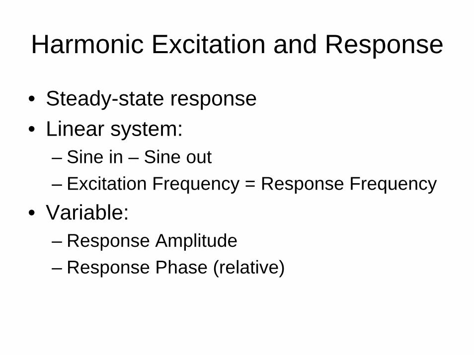
Harmonic Excitation and Response

• Steady-state response• Linear system:

– Sine in – Sine out– Excitation Frequency = Response Frequency

• Variable:– Response Amplitude– Response Phase (relative)

• Equation of Motion

• Harmonic Excitation

• Harmonic Response

mx(t) + cx(t) + kx(t) = F (t)

F (t) = F0 cos(ωt)

x(t) = X cos(ωt− φ)= X cosφ cos(ωt) +X sinφ sin(ωt)

= Xc cos(ωt) +Xs sin(ωt)

X = X2c +X

2s tanφ = Xs

Xc

−mω2Xc + cωXs + kXc = F0−mω2Xs − cωXc + kXs = 0

Xc =(k −mω2)F0

(k −mω2)2 + (cω)2

Xs =(cω)F0

(k −mω2)2 + (cω)2

X =F0p

(k −mω2)2 + (cω)2φ = tan−1

cω

k −mω2

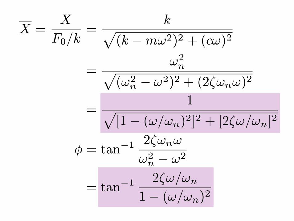
X =X

F0/k=

kp(k −mω2)2 + (cω)2

=ω2np

(ω2n − ω2)2 + (2ζωnω)2

=1p

[1− (ω/ωn)2]2 + [2ζω/ωn]2

φ = tan−12ζωnω

ω2n − ω2

= tan−12ζω/ωn

1− (ω/ωn)2

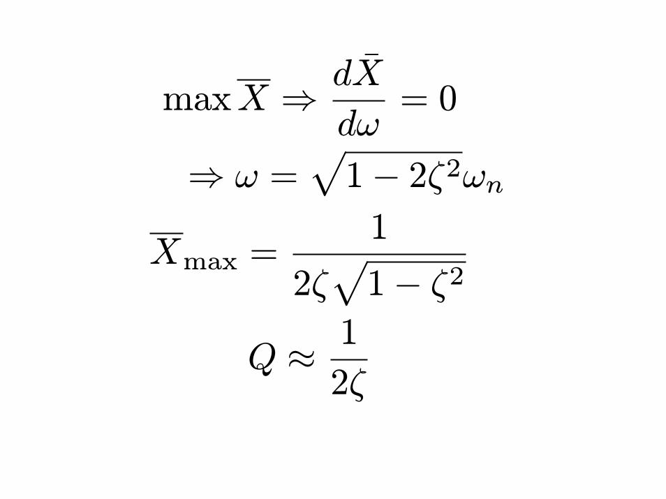
maxX ⇒ dX

dω= 0

⇒ ω = 1− 2ζ2ωnXmax =

1

2ζ 1− ζ2

Q ≈ 1

2ζ

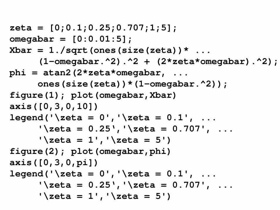
zeta = [0;0.1;0.25;0.707;1;5];omegabar = [0:0.01:5];Xbar = 1./sqrt(ones(size(zeta))* ...

(1-omegabar.^2).^2 + (2*zeta*omegabar).^2);phi = atan2(2*zeta*omegabar, ...

ones(size(zeta))*(1-omegabar.^2));figure(1); plot(omegabar,Xbar)axis([0,3,0,10])legend('\zeta = 0','\zeta = 0.1', ...

'\zeta = 0.25‘,'\zeta = 0.707', ... '\zeta = 1','\zeta = 5')

figure(2); plot(omegabar,phi)axis([0,3,0,pi])legend('\zeta = 0','\zeta = 0.1', ...

'\zeta = 0.25‘,'\zeta = 0.707', ... '\zeta = 1','\zeta = 5')

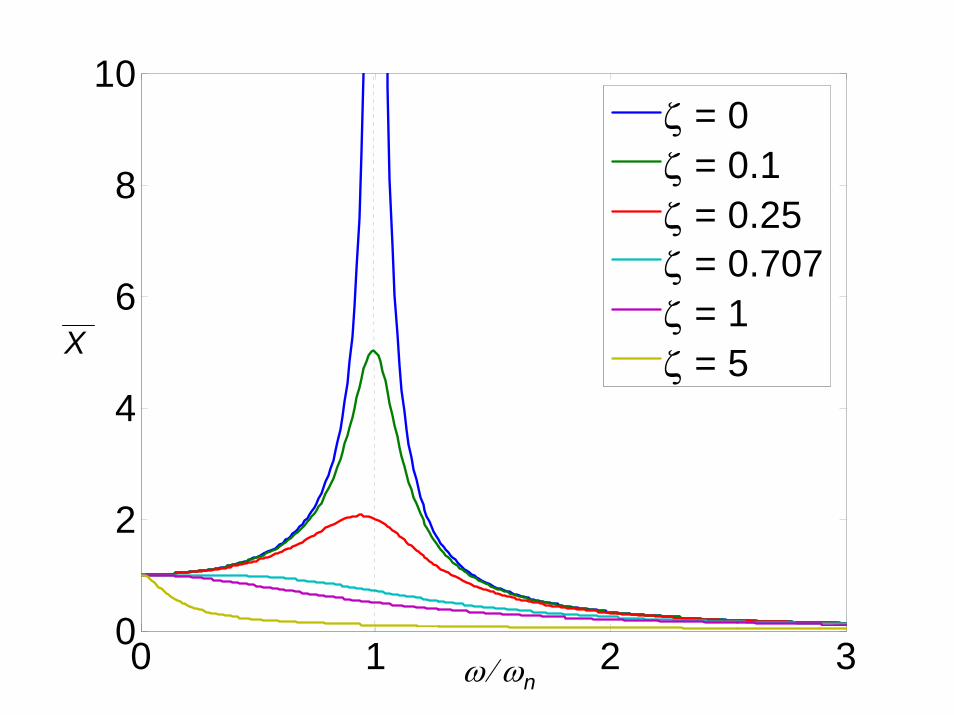
0 1 2 30

2

4

6

8

10ζ = 0ζ = 0.1ζ = 0.25ζ = 0.707ζ = 1ζ = 5

ω/ ωn

X

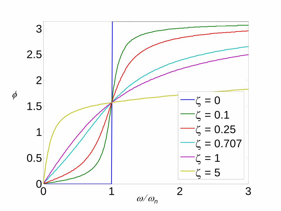
0 1 2 30

0.5

1

1.5

2

2.5

3

ζ = 0ζ = 0.1ζ = 0.25ζ = 0.707ζ = 1ζ = 5

ω/ ωn

φ

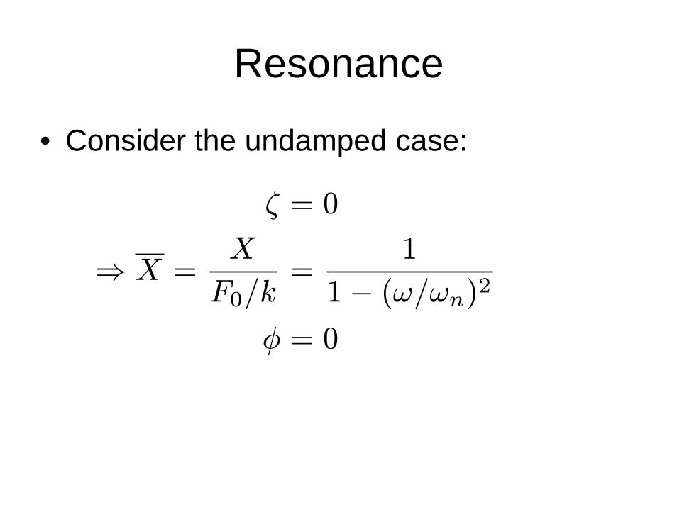
Resonance

• Consider the undamped case:

ζ = 0

⇒ X =X

F0/k=

1

1− (ω/ωn)2φ = 0

0 1 2 3-10

-5

0

5

10

ω/ ωn

X

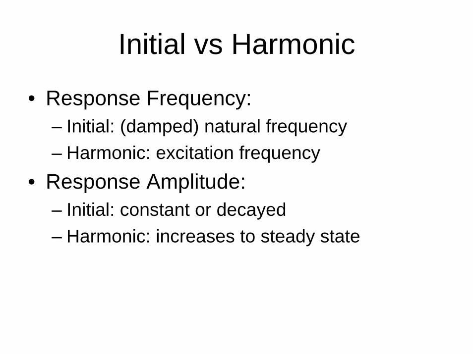
Initial vs Harmonic

• Response Frequency: – Initial: (damped) natural frequency– Harmonic: excitation frequency

• Response Amplitude:– Initial: constant or decayed– Harmonic: increases to steady state

clear allA_undamped = [0 1;-4 0];A_damped = [0 1;-4 -0.2];B = [0;1];C = [1 0];D = [0];mysys_undamped = ss(A_undamped,B,C,D);mysys_damped = ss(A_damped,B,C,D);t = 0:0.1:50;U_resonance = cos(2*t);U_non = cos(t);lsim(mysys_undamped,mysys_damped,U_resonance,t)title('Harmonic response at Resonance')legend('excitation','undamped','damped')lsim(mysys_undamped,mysys_damped,U_non,t)title('Harmonic response at other frequencies')legend('excitation','undamped','damped')

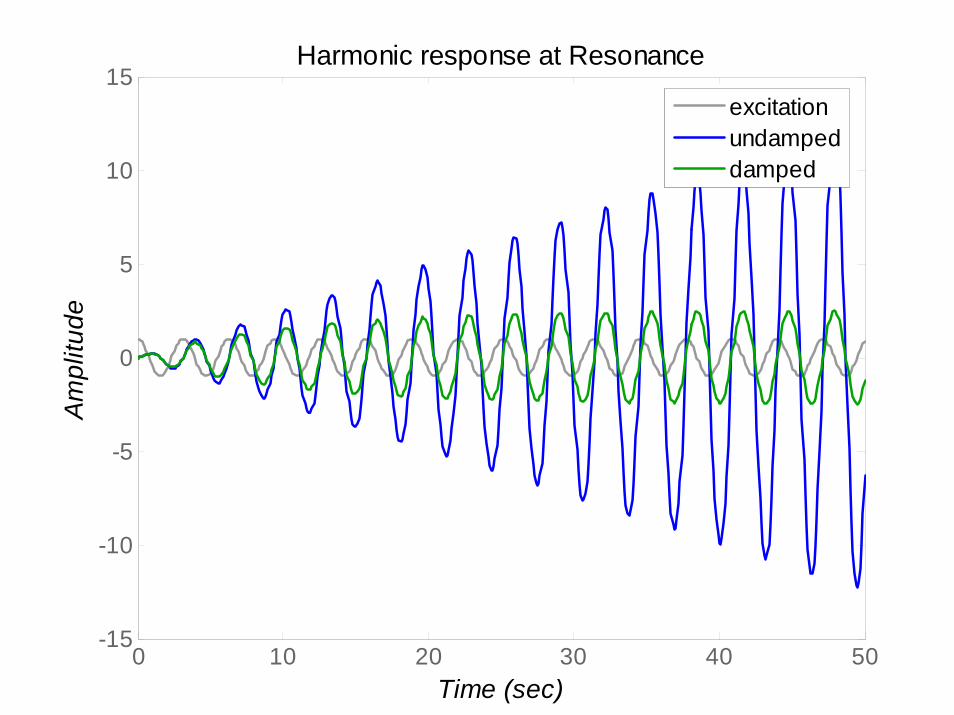
0 10 20 30 40 50-15

-10

-5

0

5

10

15Harmonic response at Resonance

Time (sec)

Am

plitu

deexcitationundampeddamped

Harmonic response at other frequencies

Time (sec)

Am

plitu

de

0 10 20 30 40 50-1

-0.8

-0.6

-0.4

-0.2

0

0.2

0.4

0.6

0.8

1excitationundampeddamped

Conclusions• At resonance: π/2 phase lag

– Undamped system oscillation amplitude increases linearly with time (no steady-state)

– Damped system oscillation amplitude increases linearly with time initially but then settles to the steady-state periodic response predicted by theory

• Off-resonance:– Undamped system oscillates at a constant amplitude

as predicted by the theory but the response is not harmonic because of the superposition of initial condition response (0 phase lag)

– Damped system behavior is similar to the undampedsystem except that the initial condition response decays in time so that the system finally oscillates at the steady-state response as predicted by theory (approximately 0 phase lag)

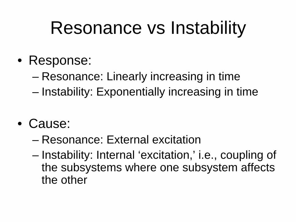
Resonance vs Instability

• Response:– Resonance: Linearly increasing in time– Instability: Exponentially increasing in time

• Cause:– Resonance: External excitation– Instability: Internal ‘excitation,’ i.e., coupling of

the subsystems where one subsystem affects the other

Response to Periodic Excitation

t

t

Tω0 =

2π

T

F(t)

F(t)

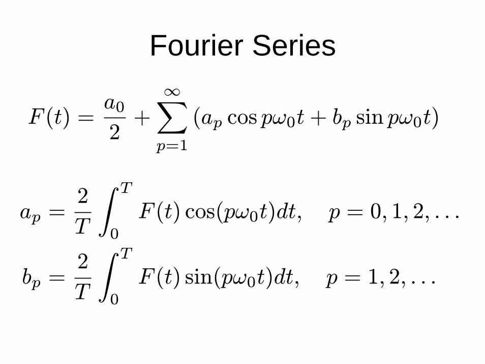
Fourier Series

F (t) =a02+

∞Xp=1

(ap cos pω0t+ bp sin pω0t)

ap =2

T

Z T

0

F (t) cos(pω0t)dt, p = 0, 1, 2, . . .

bp =2

T

Z T

0

F (t) sin(pω0t)dt, p = 1, 2, . . .

t

A

T

F(t)

ap =2

T

ÃZ T4

0

A cos(pω0t)dt

+

Z 3T4

T4

(−A) cos(pω0t)dt

+

Z T

3T4

A cos(pω0t)dt

!, p = 0, 1, 2, . . .

For odd p:

ap =A

pπ

h³(−1) p−12 − 0

´−³−(−1) p−12 − (−1) p−12

´+³0−

³−(−1) p−12

´´i=4A

pπ(−1) p−12 , p = 1, 3, 5, . . .

ap = 0, p = 0, 2, 4, . . .For even p:

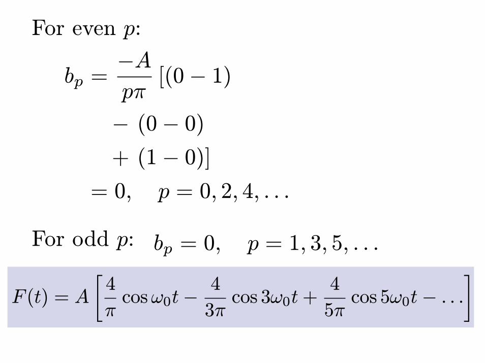
For even p:

bp =−Apπ

[(0− 1)

− (0− 0)+ (1− 0)]

= 0, p = 0, 2, 4, . . .

For odd p: bp = 0, p = 1, 3, 5, . . .

F (t) = A

∙4

πcosω0t−

4

3πcos 3ω0t+

4

5πcos 5ω0t− . . .

¸

syms tomega_0 = 2*pi;A = 1;F1 = (4*A/pi)*cos(omega_0*t);F2 = (4*A/pi)*cos(omega_0*t) ...

- (4*A/pi/3)*cos(3*omega_0*t);F10 = 0;for p = 1:2:19

F10 = F10+(-1)^((p-1)/2)*(4*A/pi/p)* ...cos(p*omega_0*t);

endplot([0,0.25,0.25,0.75,0.75,1.25, ...

1.25,1.75,1.75,2.25,2.25,2.75,2.75,3.0], ...[1,1,-1,-1,1,1,-1,-1,1,1,-1,-1,1,1],'k')

hold onezplot(F1,[0,3])ezplot(F2,[0,3])ezplot(F10,[0,3])hold off

0 1 2 3

-1

-0.5

0

0.5

1

t

Fourier Series Demonstration

exact1 term2 terms10 terms

Steady-State Responsex(t) =

1

k

a02

+∞Xp=1

apkXp cos(pω0t− φp)

+∞Xp=1

bpkXp sin(pω0t− φp)

Xp =1p

[1− (pω0/ωn)2]2 + [2ζpω0/ωn]2

φp = tan−1 2ζpω0/ωn1− (pω0/ωn)2

clear allsyms tomega_0 = 2*pi;A = 1;k=1;omega_n = pi;zeta = 0.1;F1 = 0;for p = 1

omegabar = p*omega_0/omega_n;Xbar_p = 1./sqrt(ones(size(zeta))* ...

(1-omegabar.^2).^2 + (2*zeta*omegabar).^2);phi_p = atan2(2*zeta*omegabar, ...

ones(size(zeta))*(1-omegabar.^2));F1 = F1+(-1)^((p-1)/2)*(4*A/pi/p)*Xbar_p/k*cos(p*omega_0*t-phi_p);

endF2 = 0;for p = 1:2:3



ones(size(zeta))*(1-omegabar.^2));F2 = F2+(-1)^((p-1)/2)*(4*A/pi/p)*Xbar_p/k*cos(p*omega_0*t-phi_p);

end

F10 = 0;for p = 1:2:19



ones(size(zeta))*(1-omegabar.^2));F10 = F10+(-1)^((p-1)/2)*(4*A/pi/p)*Xbar_p/k*cos(p*omega_0*t-

phi_p);endezplot(F1,[0,3])hold onezplot(F2,[0,3])ezplot(F10,[0,3])hold offtitle('Convergence of Periodic Response')ylabel('x(t)')

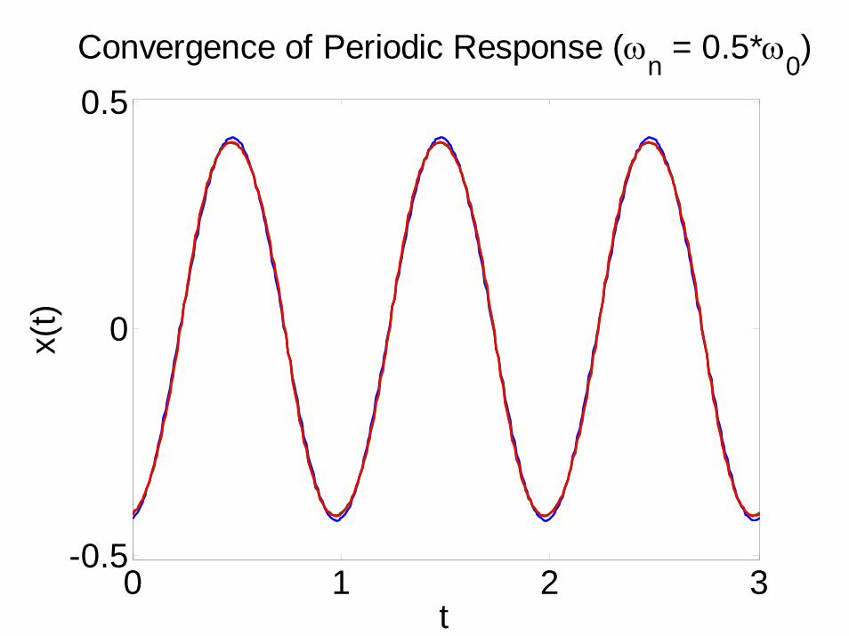
0 1 2 3-0.5

0

0.5

t

Convergence of Periodic Response (ωn = 0.5*ω0)x(

t)

0 1 2 3-3

-2

-1

0

1

2

3

t

Convergence of Periodic Response (ωn = 4.9*ω0)x(

t)

SDOF SMD - Periodic Response - Harmonic · PDF fileHarmonic Excitation and Response •...

Documents

Transcript of SDOF SMD - Periodic Response - Harmonic · PDF fileHarmonic Excitation and Response •...