users.clas.ufl.eduusers.clas.ufl.edu/llkkll/law&soc/trevino.durkheim.pdf · users.clas.ufl.edu

SDM Model Evaluation
Supplemental Discussion 8 November 2010. Based mostly on Franklin, 2010, Chapter 9

Modeling• All models have errors – they are simplifications
• A valid model is “…acceptable for its intended use because it meets specified performance requirements (Rykiel 1996).”
• “Performance can be measured by a number of criteria (Morrison et al. 1998).”
• SDM have been evaluated mostly on the basis of predictive performance.
• “Other criteria”…are also important– Ecological realism
– Spatial pattern of error
– Model credibility
References for Previous Slide
• Rykiel, E.J., Jr. 1996. Testing ecological models: the meaning of validation. Ecological Modelling 90:229-244.
• Morrison, M.L., B.G. Marcot and R.W. Mannan. 1998. Wildlife-Habitat Relationships: Concepts and Application. 2nd ed. University of Wisconsin Press. Madison.

Types of Errors
• Model error– Conceptualization and Specification– Logic– Function form
• Statistical error– Measurement error
• Systematic or Random• Inherent uncertainty of measurement• Inherent stochasticity (roll of the dice)• blunders
– Natural variation
• In SDM, all of these can cause “error.”

Error in Physics
Carlo Rubbia, 1984 Nobel Prize in Physics for Discovering W and Z bosons

Table 9.1 in Franklin (2010) Criteria for evaluating SDM – different kinds of uncertainty.
Modeling Step
Criterion Description
Conceptualformulation
Precision Ability to replicate system parameters
Specification Does the model address the problem?
Ecological Realism
Is the conceptual formulation consistent with ecological theory?
Statistical formulation
Realism Account for relevant variables and relationships?
Verification Is the model logic correct?
Model calibration
Calibration Parameter estimation or model fitting and selection
Model evaluation
Validity, performance
Produces empirically correct predictions acceptably accurate for the intended application
Appeal, credibility
Accepted by users, matches user intuition, sufficient degree of belief

Evaluating Predictive Performance of SDM 1: Sampling
• Optimal: Evaluate with new or independent data– New field work (prospective sampling)
– New location (geographically and environmentally representative)
• “Training” vs. “evaluation” or “testing” subsets– Rule of thumb: proportion of testing data should be 1/(1 +
sqrt(p-1)) where p is the number of predictors.
– p = 2 - 50:50; p = 5 – 67:33; p > 10 – 75:25
– “k-fold”; multiple splits, multiple evaluations
– Bootstrap sampling (with replacement)
• Other sample area geographically and environmentally similar (“representative”) of the study area.
Evaluating Predictive Performance of SDM 1: Measures
• For continuous variables
– R2
– RMSE
– Mean (absolute, percent) error
– Etc.
• But for SDM, need measures of categorical, ordinal, or probabilistic results.

Evaluating Predictive Performance of SDM 1: SDM Measures
• Probabilistic Categorical – Logistic regression, maximum likelihood, CART,
ANN, MaxEnt
– Threshold
– Maximum of multiple inputs
• Threshold-dependent measures of accuracy– Contingency (or Confusion) table
– Choosing a threshold (probability value above which a case is predicted to be positive)

Thresholds, Categories, and Error Costs
• Omission errors – False Positive (predicting absences incorrectly, or predicting unsuitable habitat incorrectly) more costly– Identifying sites for species reintroduction
– Identifying sites more susceptible to invasives.
• Commission errors – False Negative (predicting presences incorrectly, or predicting suitable habitat incorrectly) more costly– Designating critical habitat for species of concern
• Optimize threshold?

Error Matrix, Contingency Table, Confusion Table
Observed
Present Absent SUM
PREDICTED Present TP (true positive)
FP (false positive)
Total Predicted Present
Absent FN (false negative)
TN (true negative)
Total Predicted Absent
Sum Total observed present
Total observedabsent
Total number of observations
Errors of omission – false negative error rateErrors of commission – false positive error rate
Measures Beyond Total Correct
• Sensitivity – percentage of actual presences predicted
• Specificity – percentage of actual absences predicted

Error Matrix (Jensen)Reference Data User's Commission
Classification Residential Commercial Wetland Forest Water Row Total Accuracy Error False +
Residential 70 5 0 13 0 88 70/88 0.80 0.20
Commercial 3 55 0 0 0 58 55/58 0.95 0.05
Wetland 0 0 99 0 0 99 99/99 1.00 0.00
Forest 0 0 4 37 0 41 37/41 0.90 0.10
Water 0 0 0 0 121 121 121/121 1.00 0.00
Column Total 73 60 103 50 121 407
Overall Accuracy 382/407
Producer's Accuracy 70/73 55/60 99/103 37/50 121/121 0.94
0.96 0.92 0.96 0.74 1.00
Omission Error 0.04 0.08 0.04 0.26 0.00 False -
1. Overall Accuracy: Number Correct in the Entire Matrix2. User’s Accuracy: Probability that a classified pixel is actually of that class;
Commission Error - Error of Inclusion; An error of commission results when a pixel is committed to an incorrect class. False Positive
3. Producer’s Accuracy: Probability of a pixel being correctly classified; Omission Error - Error of Exclusion; An error of omission results when a pixel is incorrectly classified into another category. The pixel is omitted from its correct category. False Negative

Kappa StatisticKhat: a discrete multivariate technique for expressing overall accuracy by comparing two sources of data. How much does the classification differ from a random matrix (H0 is Kappa = 0)?
N S xii - S (xi+ * x+i)
Khat = ---------------------------------------
N2 - S (xi+ * x+i)
where: N = number of observationsr = rows in matrixxii = number of observations in row i and column i.Xi+ and x+i = marginal totals for row i and column i, respectively

• Measure Calculation• Prevalence Presences / Total observations• Sensitivity TP / (TP + FN)• False Neg. Rate 1 – Sensitivity• Specificity TN / (TN + FP)• False Pos. Rate 1 – Specificity• Percent Correct (TP + TN) / n• Positive Pred. Power TP / (TP + FP)• Odds Ratio (TP x TN) / (FP X FN)• Kappa• True Skill Statistic 1 – maximize (Sensitivity
+ Specificity)
Error Matrix, Contingency Table, Confusion Table Analysis
Sensitivity – percentage of actual presences predictedSpecificity – percentage of actual absences predicted
Threshold Choice
• Minimum probability for which a case is predicted to be positive. (Often 0.5).
• Effect of threshold on omission and commission error rates depends on the prevalence (of positives) in the sample.
– Threshold at FP = FN is about the level of prevalence, e.g. if 10% of samples are positive, the threshold at which sensitivity = specificity is about 0.1.
• Optimal threshold?
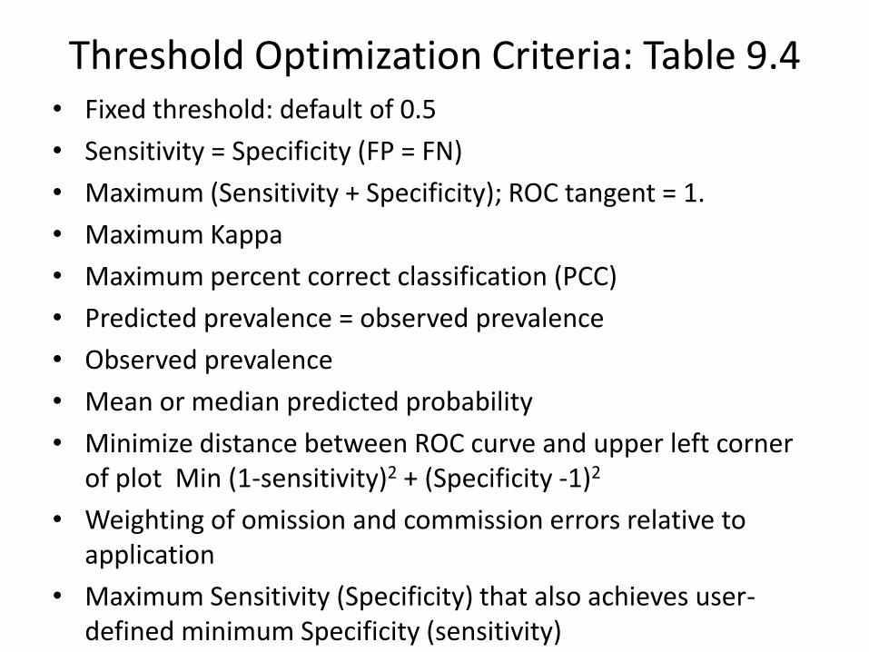
Threshold Optimization Criteria: Table 9.4• Fixed threshold: default of 0.5
• Sensitivity = Specificity (FP = FN)
• Maximum (Sensitivity + Specificity); ROC tangent = 1.
• Maximum Kappa
• Maximum percent correct classification (PCC)
• Predicted prevalence = observed prevalence
• Observed prevalence
• Mean or median predicted probability
• Minimize distance between ROC curve and upper left corner of plot Min (1-sensitivity)2 + (Specificity -1)2
• Weighting of omission and commission errors relative to application
• Maximum Sensitivity (Specificity) that also achieves user-defined minimum Specificity (sensitivity)
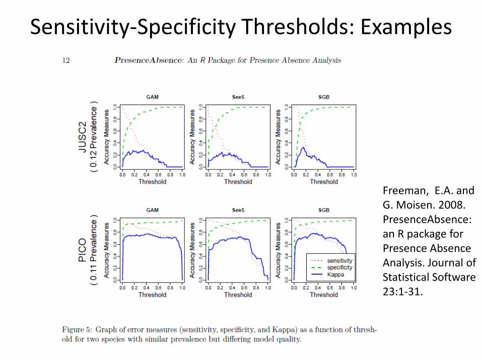
Sensitivity-Specificity Thresholds: Examples
Freeman, E.A. and G. Moisen. 2008. PresenceAbsence: an R package for Presence Absence Analysis. Journal of Statistical Software 23:1-31.
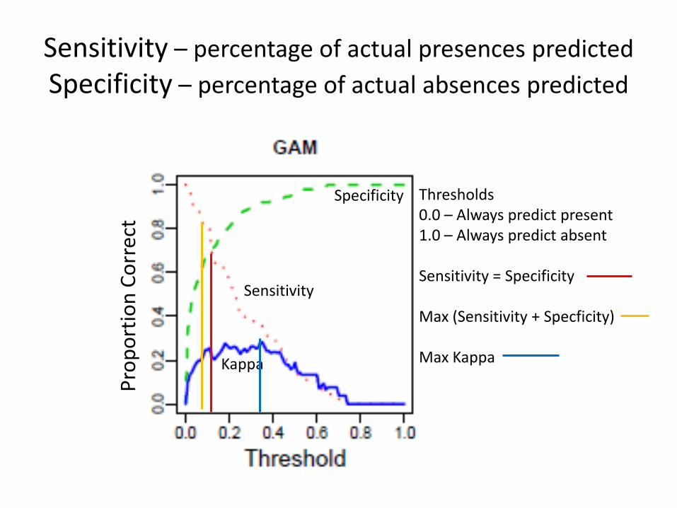
Sensitivity – percentage of actual presences predicted
Specificity – percentage of actual absences predicted
Thresholds0.0 – Always predict present1.0 – Always predict absent
Sensitivity = Specificity
Max (Sensitivity + Specficity)
Max Kappa
Specificity
Sensitivity
Kappa
Pro
po
rtio
n C
orr
ect

Threshold Independent measures: AUC/ROC Curves
• AUC – Area under the curve of the
• ROC – Receiver-operating characteristic; plot of sensitivity vs 1-specificity.
Straight line – difficult to classify, totally random
Sensitivity – percentage of actual presences predicted
Specificity – percentage of actual absences predicted1-Specificity is false positive rate
Pretty good classifier
Excellent classifier
ROC Curves AUC = 0.5
AUC = 0.8
AUC = 0.95
Rule of Thumb0.5 – 0.7 low0.7 – 0.9 moderate> 0.9 high

AUC
• AUC not strongly affected by species prevalence
• When it is affected, it is due to species ecology
– More difficult to discriminate unsuitable habitat for generalist species.
• I’ll leave the biology to you

Other Accuracy Measures
• Correlation
– Biserial correlation: observed presence/absence vs. probability of presence
– Rank correlation (Concordance Index)
• Calibration

Presence-Only Models
• Pseudo-absences
• Threshold that minimizes omission (false negatives) errors and minimizes area predicted to be suitable.
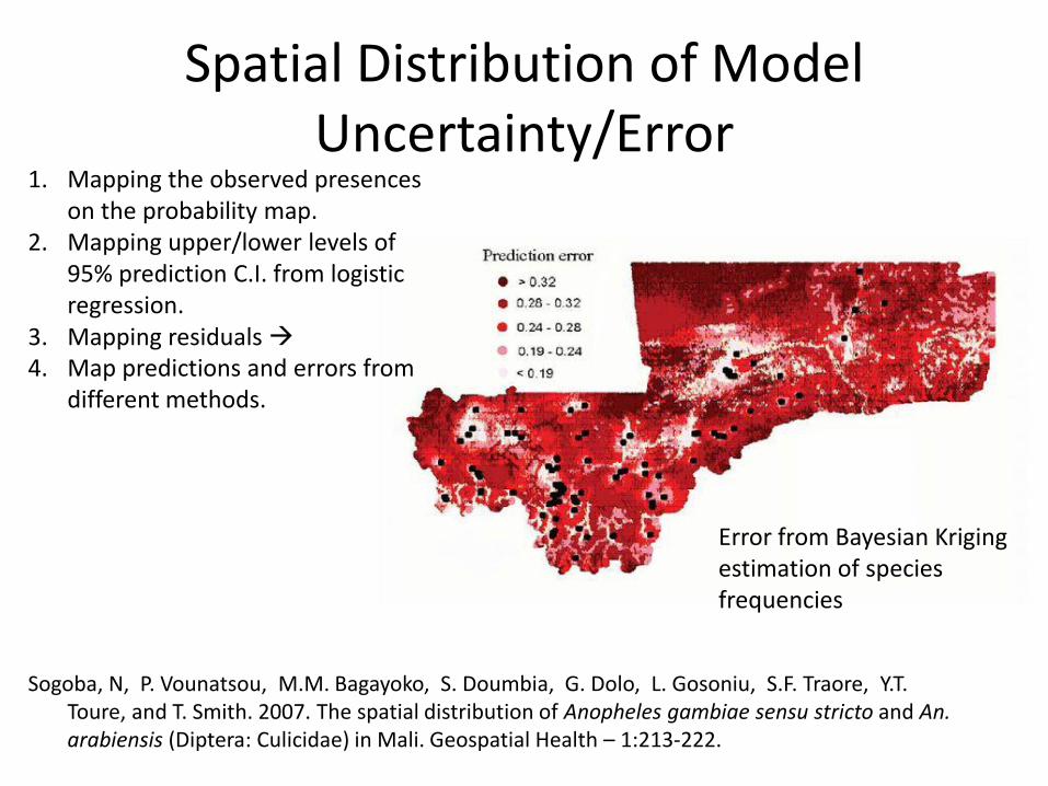
Spatial Distribution of Model Uncertainty/Error
Sogoba, N, P. Vounatsou, M.M. Bagayoko, S. Doumbia, G. Dolo, L. Gosoniu, S.F. Traore, Y.T. Toure, and T. Smith. 2007. The spatial distribution of Anopheles gambiae sensu stricto and An. arabiensis (Diptera: Culicidae) in Mali. Geospatial Health – 1:213-222.
1. Mapping the observed presences on the probability map.
2. Mapping upper/lower levels of 95% prediction C.I. from logistic regression.
3. Mapping residuals 4. Map predictions and errors from
different methods.
Error from Bayesian Krigingestimation of species frequencies

Now on to YOU