SDH/SONET Explained in - tron-inter.net...connection-oriented networks, e.g. PDH, SDH, SONET, OTN,...

SDH/SONETExplained inFunctional Models

TEAM LinG

SDH/SONETExplained inFunctional ModelsModeling the Optical TransportNetwork

Huub van HelvoortNetworking Consultant, the Netherlands

Copyright # 2005 John Wiley & Sons Ltd, The Atrium, Southern Gate, Chichester,West Sussex PO19 8SQ, England

Telephone (+44) 1243 779777

Email (for orders and customer service enquiries): [email protected] our Home Page on www.wiley.com

All Rights Reserved. No part of this publication may be reproduced, stored in aretrieval system or transmitted in any form or by any means, electronic, mechanical,photocopying, recording, scanning or otherwise, except under the terms of theCopyright, Designs and Patents Act 1988 or under the terms of a licence issued by theCopyright Licensing Agency Ltd, 90 Tottenham Court Road, London W1T 4LP, UK, withoutthe permission in writing of the Publisher. Requests to the Publisher shouldbe addressed to the Permissions Department, John Wiley & Sons Ltd, The Atrium, SouthernGate, Chichester, West Sussex PO19 8SQ, England, or emailed [email protected], or faxed to (+44) 1243 770620.

Designations used by companies to distinguish their products are often claimed as trade-marks. All brand names and product names used in this book are trade names, service marks,trademarks or registered trademarks of their respective owners. The Publisher is notassociated with any product or vendor mentioned in this book.

This publication is designed to provide accurate and authoritative information in regard to thesubject matter covered. It is sold on the understanding that the Publisher is not engaged inrendering professional services. If professional advice or other expert assistance is required,the services of a competent professional should be sought.

Other Wiley Editorial Offices

John Wiley & Sons Inc., 111 River Street, Hoboken, NJ 07030, USA

Jossey-Bass, 989 Market Street, San Francisco, CA 94103-1741, USA

Wiley-VCH Verlag GmbH, Boschstr. 12, D-69469 Weinheim, Germany

John Wiley & Sons Australia Ltd, 42 McDougall Street, Milton, Queensland 4064, Australia

John Wiley & Sons (Asia) Pte Ltd, 2 Clementi Loop # 02-01, Jin Xing Distripark, Singapore129809

John Wiley & Sons Canada Ltd, 22 Worcester Road, Etobicoke, Ontario, Canada M9W 1L1

Wiley also publishes its books in a variety of electronic formats. Some content that appears inprint may not be available in electronic books.

British Library Cataloguing in Publication Data

A catalogue record for this book is available from the British Library

ISBN 0-470-09123-1

Typeset in 10/12pt Palatino by Thomson Press (India) Limited, New Delhi, India.Printed and bound in Great Britain by Antony Rowe Ltd, Chippenham, Wiltshire.This book is printed on acid-free paper responsibly manufactured from sustainable forestryin which at least two trees are planted for each one used for paper production.

http://www.wiley.com

To my wife Leontine for her support and patience,and in memory of my parents

Contents

Preface . . . . . . . . . . . . . . . . . . . . . . . . . . . . . . . . . . . . . . . . . . . . . xi

Acknowledgements . . . . . . . . . . . . . . . . . . . . . . . . . . . . . . . . . . . xiii

Abbreviations . . . . . . . . . . . . . . . . . . . . . . . . . . . . . . . . . . . . . . . xv

1 Introduction . . . . . . . . . . . . . . . . . . . . . . . . . . . . . . . . . . . . . 11.1 History . . . . . . . . . . . . . . . . . . . . . . . . . . . . . . . . . . . . . 11.2 Justification. . . . . . . . . . . . . . . . . . . . . . . . . . . . . . . . . . 21.3 Remarks on the concept . . . . . . . . . . . . . . . . . . . . . . . . 41.4 Standards structure . . . . . . . . . . . . . . . . . . . . . . . . . . . 9

2 Functional modeling . . . . . . . . . . . . . . . . . . . . . . . . . . . . . . 112.1 Functional architecture of transport networks . . . . . . . 112.2 Functional model requirements . . . . . . . . . . . . . . . . . . 142.3 Functional model basic structure . . . . . . . . . . . . . . . . . 15

2.3.1 Architectural components . . . . . . . . . . . . . . . . . 152.3.2 Topological components . . . . . . . . . . . . . . . . . . 20

2.4 Functional model detailed structure . . . . . . . . . . . . . . . 222.4.1 Transport entities. . . . . . . . . . . . . . . . . . . . . . . . 222.4.2 Transport processing functions . . . . . . . . . . . . . 272.4.3 Reference points . . . . . . . . . . . . . . . . . . . . . . . . 322.4.4 Components comparison . . . . . . . . . . . . . . . . . . 35

2.5 Client/server relationship. . . . . . . . . . . . . . . . . . . . . . . 362.5.1 Multiplexing . . . . . . . . . . . . . . . . . . . . . . . . . . . 382.5.2 Inverse multiplexing . . . . . . . . . . . . . . . . . . . . . 39

2.6 Layer network interworking. . . . . . . . . . . . . . . . . . . . . 412.7 Linking the functional model and the information

model . . . . . . . . . . . . . . . . . . . . . . . . . . . . . . . . . . . . . . 43

2.8 Application of concepts to network topologiesand structures. . . . . . . . . . . . . . . . . . . . . . . . . . . . . . . . 452.8.1 PDH supported on SDH layer networks . . . . . . 452.8.2 Inverse multiplexing transport. . . . . . . . . . . . . . 48

3 Partitioning and layering. . . . . . . . . . . . . . . . . . . . . . . . . . . 493.1 Layering concept . . . . . . . . . . . . . . . . . . . . . . . . . . . . . 493.2 Partitioning concept . . . . . . . . . . . . . . . . . . . . . . . . . . . 51

3.2.1 Sub-network partitioning . . . . . . . . . . . . . . . . . . 513.2.2 Flow domain partitioning . . . . . . . . . . . . . . . . . 553.2.3 Link partitioning . . . . . . . . . . . . . . . . . . . . . . . . 563.2.4 Access group partitioning . . . . . . . . . . . . . . . . . 58

3.3 Concept applications . . . . . . . . . . . . . . . . . . . . . . . . . . 593.3.1 Application of the layering concept . . . . . . . . . . 593.3.2 Application of the partitioning concept . . . . . . . 59

4 Expansion and reduction . . . . . . . . . . . . . . . . . . . . . . . . . . . 614.1 Expansion of layer networks . . . . . . . . . . . . . . . . . . . . 61

4.1.1 Expansion of the path layer network . . . . . . . . . 624.1.2 Expansion of the transmission media layer . . . . 624.1.3 Expansion of specific layer networks

into sublayers . . . . . . . . . . . . . . . . . . . . . . . . . . 634.2 General principles of expansion of layers . . . . . . . . . . . 64

4.2.1 Adaptation expansion . . . . . . . . . . . . . . . . . . . . 644.2.2 Trail termination expansion . . . . . . . . . . . . . . . . 654.2.3 Connection point expansion . . . . . . . . . . . . . . . 65

4.3 Reduction of detail . . . . . . . . . . . . . . . . . . . . . . . . . . . . 66

5 Adaptation functions . . . . . . . . . . . . . . . . . . . . . . . . . . . . . . 695.1 Generic adaptation function . . . . . . . . . . . . . . . . . . . . . 695.2 Adaptation function examples . . . . . . . . . . . . . . . . . . . 76

5.2.1 The Sn/Sm_A function . . . . . . . . . . . . . . . . . . . 765.2.2 The OCh/RSn_A function . . . . . . . . . . . . . . . . . 835.2.3 The LCAS capable Sn–X–L/ETH_A function. . . 885.2.4 GFP mapping in the Sn–X/

<client>_A function . . . . . . . . . . . . . . . . . . . . . 96

6 Trail termination functions . . . . . . . . . . . . . . . . . . . . . . . . . 996.1 Generic trail termination function. . . . . . . . . . . . . . . . . 996.2 Trail termination function examples . . . . . . . . . . . . . . . 105

6.2.1 The Sn_TT function . . . . . . . . . . . . . . . . . . . . . . 105

viii Contents

6.2.2 The OCh_TT function . . . . . . . . . . . . . . . . . . . . 1126.2.3 The ETH_FT function . . . . . . . . . . . . . . . . . . . . 117

7 Connection functions. . . . . . . . . . . . . . . . . . . . . . . . . . . . . . 1237.1 Generic connection function . . . . . . . . . . . . . . . . . . . . . 1237.2 Connection function example . . . . . . . . . . . . . . . . . . . . 127

7.2.1 VC–n layer connection function Sn_C . . . . . . . . 1277.2.2 ETH flow domain . . . . . . . . . . . . . . . . . . . . . . . 134

7.3 Connection matrix examples . . . . . . . . . . . . . . . . . . . . 1357.3.1 Connection matrix example for full

connectivity . . . . . . . . . . . . . . . . . . . . . . . . . . . . 1357.3.2 Connection matrix example for two groups. . . . 1377.3.3 Connection matrix example for three groups. . . 138

8 Connection supervision . . . . . . . . . . . . . . . . . . . . . . . . . . . . 1438.1 Quality of Service . . . . . . . . . . . . . . . . . . . . . . . . . . . . . 1438.2 Connection monitoring methods . . . . . . . . . . . . . . . . . 144

8.2.1 Inherent monitoring. . . . . . . . . . . . . . . . . . . . . . 1458.2.2 Non-intrusive monitoring . . . . . . . . . . . . . . . . . 1458.2.3 Intrusive monitoring . . . . . . . . . . . . . . . . . . . . . 1478.2.4 Sublayer monitoring . . . . . . . . . . . . . . . . . . . . . 148

8.3 Connection monitoring applications . . . . . . . . . . . . . . . 1498.3.1 Monitoring of unused connections. . . . . . . . . . . 1508.3.2 Tandem connection monitoring . . . . . . . . . . . . . 151

9 Protection models . . . . . . . . . . . . . . . . . . . . . . . . . . . . . . . . 1559.1 Introduction . . . . . . . . . . . . . . . . . . . . . . . . . . . . . . . . . 1559.2 Protection . . . . . . . . . . . . . . . . . . . . . . . . . . . . . . . . . . . 159

9.2.1 Trail protection . . . . . . . . . . . . . . . . . . . . . . . . . 1609.2.2 Sub-network connection protection . . . . . . . . . . 171

10 Compound functional models and their decomposition. . . 17910.1 LCAS disabled VCAT functions . . . . . . . . . . . . . . . . . . 179

10.1.1 Sn–Xv trail termination function . . . . . . . . . . . . 18110.1.2 Sn–Xv/Sn–X adaptation function. . . . . . . . . . . . 18310.1.3 Sn–X trail termination function . . . . . . . . . . . . . 18910.1.4 Sn trail termination function . . . . . . . . . . . . . . . 192

10.2 LCAS-capable VCAT functions. . . . . . . . . . . . . . . . . . . 19310.2.1 Sn–Xv–L layer trail termination function . . . . . . 19310.2.2 Sn–Xv/Sn–X–L adaptation function . . . . . . . . . . 19410.2.3 Sn–X–L trail termination function . . . . . . . . . . . 200

Contents ix

10.2.4 Sn trail termination function . . . . . . . . . . . . . . . 20410.2.5 Sn–X–L to client signal adaptation function . . . . 204

10.3 VCAT network model . . . . . . . . . . . . . . . . . . . . . . . . . 20710.4 S4–Xc to S4–Xc interworking function . . . . . . . . . . . . . 20810.5 VCAT-CCAT interworking network model . . . . . . . . . 216

11 Example functional models to exercise . . . . . . . . . . . . . . . . 21911.1 Device level functional model . . . . . . . . . . . . . . . . . . . 21911.2 Equipment detailed functional model. . . . . . . . . . . . . . 22111.3 Network element functional model . . . . . . . . . . . . . . . 22511.4 Trail connection model . . . . . . . . . . . . . . . . . . . . . . . . . 23311.5 Synchronization network model . . . . . . . . . . . . . . . . . . 240

11.5.1 Synchronization methods. . . . . . . . . . . . . . . . . . 24011.5.2 Synchronization network architecture . . . . . . . . 241

11.6 OTN network element model . . . . . . . . . . . . . . . . . . . . 24411.7 Data transport model . . . . . . . . . . . . . . . . . . . . . . . . . . 246

11.7.1 Equipment models for GFP . . . . . . . . . . . . . . . . 24611.7.2 Ethernet tributary port. . . . . . . . . . . . . . . . . . . . 24811.7.3 IP router port. . . . . . . . . . . . . . . . . . . . . . . . . . . 25011.7.4 SAN tributary port . . . . . . . . . . . . . . . . . . . . . . 250

11.8 Ethernet layer network model . . . . . . . . . . . . . . . . . . . 25111.8.1 ETY layer network terminology. . . . . . . . . . . . . 25111.8.2 ETH layer network terminology . . . . . . . . . . . . 25211.8.3 Ethernet layer network example . . . . . . . . . . . . 253

11.9 MPLS layer network model . . . . . . . . . . . . . . . . . . . . . 25511.9.1 MPLS layer network terminology . . . . . . . . . . . 25511.9.2 MPLS layer network example . . . . . . . . . . . . . . 256

Glossary. . . . . . . . . . . . . . . . . . . . . . . . . . . . . . . . . . . . . . . . . . . . 259

References . . . . . . . . . . . . . . . . . . . . . . . . . . . . . . . . . . . . . . . . . . 275

Index . . . . . . . . . . . . . . . . . . . . . . . . . . . . . . . . . . . . . . . . . . . . . . 279

x Contents

Preface

The use of a natural language to describe the functionality in transmis-sion networks and transport equipment will lead to misinterpretationof the written requirements and cause equipment not to interoperate.The growth in complexity of the functionality and diversity of theoptical transport network capabilities to be described, and the numberof different users, for example, system engineers, marketing, custo-mers, developers, standards representatives, meant that it was neces-sary to develop and define a common language.

In this book I describe this language, i.e. the methodology that isused to model the functionality of transport networks and transportequipment. The functional modeling methodology is applicable inconnection-oriented networks, e.g. PDH, SDH, SONET, OTN, as wellas connectionless networks, e.g. Ethernet, MPLS. The emphasis in thisbook is on the explanation of the functional modeling methodologyand its use as a description tool. Examples are provided to help thereader in understanding modeling technique.

Based on my experience with the use of functional models over thepast ten years, I expect that many readers of this book will be SystemEngineers and Functional Architects who are employed by OpticalTransport Network operators, Optical Transport equipment manufac-turers and device manufacturers, especially those who are responsiblefor transport-related functionality at Networking or Network Elementlevel. It will help them to use and develop functional models in thearea of their responsibility.

I assume that optical network, equipment and device developmentengineers as well as system verification, system test and interoper-ability test engineers will use this book as a guideline.

Finally, I hope that this book will be used by students in telecom-munications technology and by members of the IEEE community as areference to acquire the skill of functional modeling.

Acknowledgements

I especially thank Eve Varma, Maarten Vissers and George Newsomefor their cooperation and for sharing my enthusiasm.

Huub van Helvoort, M.S.E.E., Senior member IEEE.

Abbreviations

AcSQ Accepted Sequence numberADM Add-Drop MultiplexerAI Adapted InformationAIS Alarm Indication Signal (i.e. Alarm Inhibit Signal)ANSI American National Standards InstituteAP Access PointAPI Access Point IdentifierAPS Automatic Protection SwitchATM Asynchronous Transport ModuleAU Administrative UnitBP Bridge ProtocolCBRx Constant BitRate signal with approximate bitrate xCCAT Contiguous conCATenationCCITT Comite Consulatif Telegraphique et Telephonique

(now ITU-T)CI Characteristic InformationCP Connection PointCRC Cyclic Redundancy CheckDCC Data Communications ChannelDCN Data Communications NetworkDXC Digital Cross-ConnectEOW Engineer Order WireETSI European Telecommunications Standards InstituteFCS Frame Check SequenceFD Flow DomainFDFr Flow Domain FragmentFEBE Far End Block ErrorFERF Far End Receive FailureFOP Failure of Protocol

FP Flow PointFPP Flow Point PoolGFP Generic Framing ProcessIEEE Institute of Electrical and Electronics EngineersIP Internet ProtocolISO International Organization for StandardizationITU-T International Telecommunications Union—

Telecommunication Standardization Sector(former CCITT)

LAN Local Area NetworkLC Link ConnectionLCAS Link Capacity Adjustment SchemeLOA Loss of AlignmentLOM Loss of Multi-frameMAC Media Access ControlMAN Metro Area NetworkMI Management InformationMND Member Not De-skewableMP Management PointMPLS Multi-Protocol Label SwitchingMS-SPRing Multiplex Section—Shared Protection RingMSn Multiplex Section of level nMSAP Multi-Service Access PlatformMSPP Multi-Service Provisioning PlatformMSSP Multi-Service Switching PlatformMSTP Multi-Service Transport PlatformMSU Member Service UnavailableMTBF Mean Time Between FailuresMTTR Mean Time To RepairNC Network ConnectionNNI Network to Network InterfaceNUT Non-pre-emptible Unprotected TrafficOAM/OA&M Operation Administration and MaintenanceOSI Open Systems InterconnectionOOS OTM Overhead SignalOSn Optical Section of level nOTM Optical Transport ModuleOTN Optical Transport NetworkPCI Protocol Control InformationPDH Plesiochronous Digital HierarchyPLC Partial Loss of payload CapacityPOH Path OverHead

xvi Abbreviations

PRC Primary Reference ClockQoS Quality of ServiceRDI Remote Defect IndicationREI Remote Error IndicationRI Remote InformationRP Remote PointRSn Regenerator Section of level nSk SinkSo SourceSAN Storage Area NetworkSD Signal DegradeSDH Synchronous Digital HierarchySDU Service Data UnitSF Signal FailSLA Service Level AgreementSNC Sub-Network ConnectionSNCP Sub-Network Connection ProtectionSNC/I SNCP using Inherent monitoringSNC/N SNCP using Non-intrusive monitoringSNC/S SNCP using Sub-layeringSONET Synchronous Optical NetworkSQ Sequence numberSQM SQ MismatchSSD Server Signal DegradedSSF Server Signal FailedSSM Synchronization Status MessagingSTM-N Synchronous Transport Module (level) NTCM Tandem Connection MonitoringTCP Termination Connection PointTFP Termination Flow PointTI Timing InformationTLC Total Loss of payload CapacityTP Timing PointTSD Trail Signal DegradedTSF Trail Signal FailTTI Trail Trace IdentifierTU Tributary UnitUNI User to Network InterfaceVC–n Virtual container (level) nVCAT Virtual conCATenationVCG Virtual Concatenation GroupWAN Wide Area Network

Abbreviations xvii

1

Introduction

A telecommunications network is a complex network that can bedescribed in a number of different ways depending on the particularpurpose of the description. In this book the optical transport networkwill be described as a network from the viewpoint of the capability totransfer information. More specifically, the functional and structuralarchitecture of optical transport networks is described independently ofthe networking technology, for example, distribution, platforms, packag-ing. The methodology used for this description is commonly referred toas functional modeling and is used in many standards documents todescribe the functional architecture of existing and evolving PDH,SDH, OTN, ATM, Ethernet and MPLS networks. The functionalmodel is also used extensively by operators to describe their networkand by manufacturers to describe their equipment or devices.

1.1 HISTORY

The development of functional models for use in telecommunicationnetworks was a combined effort of network operators and equipmentmanufacturers. After an extensive analysis of existing transport net-work structures, the functional modeling methodology was firstintroduced in the standards documents of the European Telecommuni-cations Standards Institute (ETSI) around 1995. In the ETSI standards themethodology was used to model the SDH network and its equipment.After the introduction and standardization in ETSI, the InternationalTelecommunications Union – Telecommunication Standardization Sector

SDH/SONET Explained in Functional Models Huub van Helvoort# 2005 John Wiley & Sons, Ltd

(ITU-T) also adapted the functional modeling in 1997. Althoughinitially used for the specification of SDH, later it was applied in thespecification of other technologies. Currently, work is in progress onmodeling Ethernet networks. There is an increased interest in theAmerican National Standards Institute (ANSI) to adopt the functionalmodel methodology in their standards.

1.2 JUSTIFICATION

There were several reasons to start the study and development of amethodology to model a transport network or equipment in a func-tional way. Some of these reasons were:

� Increased complexity. Owing to the natural growth of optical trans-port networks and equipment, the contained functionalityincreased as well.

� Increased variety. Owing to the growth in complexity, the number ofrequired functions also increased as well as the number of possiblecombinations of these functions.

� Multiple applications. The same transport equipment is labeleddifferently, e.g. multiplexer, cross-connect, line system, dependingon the application in the network topology.

� Written requirements. Generally, in a natural language, there havethe following disadvantages:- no common language; requires translation- voluminous; easy to lose overview- inconsistent; often dependent on the writer’s background- ambiguous; uses a natural language- incomplete.

These reasons meant that it became more and more difficult tomanage the transport network and equipment. It was almost impos-sible to guarantee the compatibility and interoperability of equipmentbased solely on written documentation. Consequently, this createdthe need for a new language that showed similarities where networksand equipment were similar and differences where they were dis-similar.

Considering the reasons mentioned above, the following require-ments were taken as input for the study to establish a new descriptionmethodology, i.e. a common language:

2 SDH/SONET Explained in Functional Models

� It should provide a flexible description of the functional architec-ture at transport network level that takes into account varyingpartitioning and layering requirements.

� It should identify functional similarities and differences in hetero-geneous technology-based layered transport network architecture.

� It should be able to produce network element functional modelsthat are traceable to and reflective of network level requirements.

� It should establish a rigorous and consistent relationship betweentransport network functional architecture and management infor-mation models.

In addition, the established methodology should have the followingcharacteristics:

� it is simple;� it is short;� it is visual;� it contains basic elements;� it provides combination rules;� it supports generic usage;� it has recursive structures;� it is implementation independent;� it is transport level independent;� it has the capability to automate generation and verification.

The result of the study is the definition and standardization of thefunctional modeling methodology. With a functional model it ispossible to present:

� Optical Transport Network capabilities, independent of actualdeployed equipments.

� Transport Equipment capabilities, independent of actual equip-ment implementation.

The unambiguous specification produced by applying the methodol-ogy will provide a unique definition of transport networks andequipment towards:

� Optical Transport Network operators;� Optical Transport Equipment and Device manufacturers;� Network Management Systems and Element Management Systems.

Introduction 3

1.3 REMARKS ON THE CONCEPT

The analysis and decomposition of existing transmission networksresulted in the definition of the atomic functions that are used in thefunctional modeling methodology. These atomic functions can be usedto compose the functional models of the same existing, legacy andfuture transmission networks.

This concept is not new. Some other technologies that have usedatomic models are listed below.

� Hardware (analog). The atomic functions used in this technologyare, for exampl, resistors, capacitors, inductors, diodes, and tran-sistors. These atomic functions can be used to model an analogcircuit or network, for example, an amplifier, a cable or even adigital circuit like an OR gate as illustrated in Figure 1.1.

� Hardware (digital). The atomic functions utilized in this technologyare, for example, AND, NAND, OR, NOR, INVERT and XOR gates.Even though these functions can be represented by the atomicfunctions of the analog hardware as shown in the previous exam-ple, in this technology they would provide too much detail andwould make the description of the digital circuit too complex. Thusthe gates are in fact compound functions representing the analog

Input A

Input B

Output A+B

+VCC

OR gate

Resistor

Inductor

Capacitor

Diode

Transistor

R1

R1

R2

Figure 1.1 electric circuit symbols and example.


hardware atomics. These atomic functions in this technology canagain be used to model a digital circuit, for example, a flip-flop,which can be used as a compound function in other models, amicroprocessor or a digital transmission function (e.g. a multiplexer,framer). Figure 1.2 shows the atomics and an example circuit.

� Software (assembly language). Even the primitives in textual formcan be considered as building blocks to describe a particularfunction. Examples of the textual atomic functions are JUMP,JMPNC, LOAD, STORE, SUB, XOR and NOP instructions. Theseatomic functions can be used to model a process. Figure 1.3 depictsa simple example. Instructions can be grouped together to formprocedures that can be CALLed and RETURNed from whenfinished; these procedures can be used as compound functions.

Assembly language is however very implementation specific;every vendor has its proprietary set of atomic models and thereare no generic assembly language atomic functions.

� Software (higher order language). The ITU-T has defined a higherorder language to provide a vendor independent programmingcapability for telecommunication processes: CHILL, the CCITTHigher Level Language (for a description, see ITU-T Rec. Z.200,1999). Another and more widespread higher order language is theC programming language (Kernighan and Ritchie, 1978). Theatomic functions are, for example, FOR, WHILE, IF-THEN-ELSE,

AND

XOR

INVERT

NOR

NAND

OR

DATA_in

CLOCK

DATA_out

FLIP-FLOP

Figure 1.2 logic symbols and example.

Introduction 5

CASE, and ASSIGNMENT. Frequently used routines can be col-lected in a library and used as compound functions. These atomicfunctions can be used to model a process, for example, the same asthe assembly language example above (see Figures 1.3 and 1.4.)

Higher order languages are independent of the implementation.There are, however, only a few (micro-) processors that can inter-pret this higher order language; a translator, or compiler, is used togenerate the implementation specific assembly language under-stood by a particular (micro-) processor.

� Process descriptions using state diagrams. The atomic functionsin this methodology (e.g. SDL Specification and Description Lan-guage, ITU-T Rec. Z.100, 2002) are STATE, INPUT, OUTPUT, TASKand DECISION. The TASK symbol may represent a procedure that

Figure 1.3 Assembly language example.


can again be specified in SDL and can be considered as a com-pound function. These atomic functions can be used to describe aprocess, for example, subscriber signaling, Link Capacity Adjust-ment Scheme (LCAS, see ITU-T Rec. G.7042, 2004). Hardware andsoftware designers can use these models when implementing aspecific process. Figure 1.5 shows an example of the graphicalrepresentation: SDL/GR. This is a part of the SDL diagram describ-ing the Source side processing in LCAS (see ITU-T Rec. G.7042,2004).

SDL also has a textual phrase representation as shown in Fig-ure 1.6: SDL/PR. Tools exist that use this text to generate thegraphical representation and and/or generate executable code fortesting purposes.

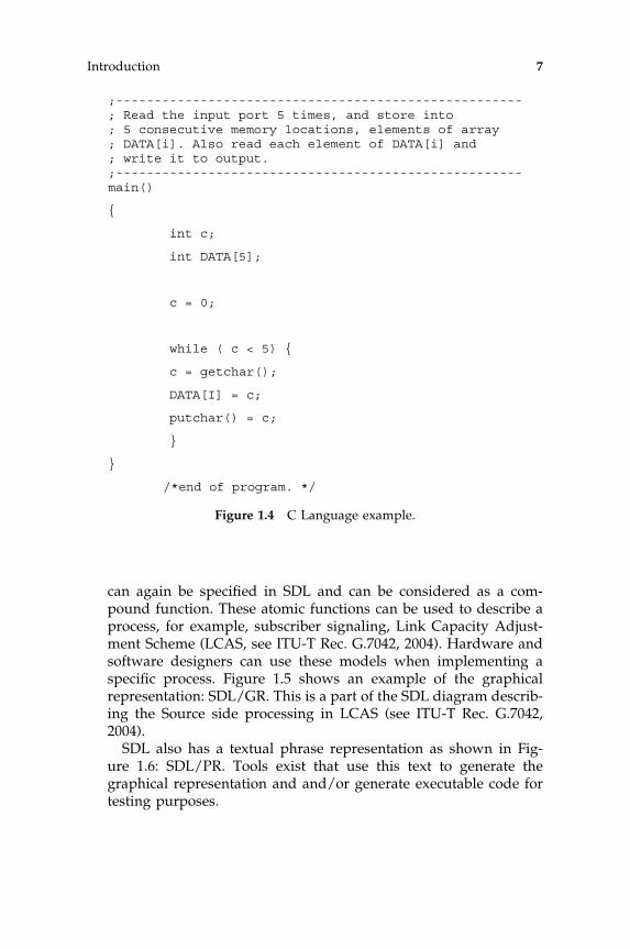
;-----------------------------------------------------; Read the input port 5 times, and store into ; 5 consecutive memory locations, elements of array ; DATA[i]. Also read each element of DATA[i] and ; write it to output. ;-----------------------------------------------------main()

{

int c;

int DATA[5];

c = 0;

while ( c < 5) {

c = getchar();

DATA[I] = c;

putchar() = c;

}

}

/*end of program. */

Figure 1.4 C Language example.

Introduction 7

MREMRFAIL

FEOSFNRM

NORM/EOS

EOS NY

DNU

FDNU

stopsendingpayload

CRSQ CNRM

SQ(i) :=SQ(i)-1

CEOS

CEOS

Sample SDL stateshowing two states and the events that cause atransition

1

state name

signal

signal

procedure

test

state symbol, an input event initiates a transition to the next state

input event, internal, external

output event, internal, external

task symbol, represents a procedure

decision symbol, selects an output based on test result

Figure 1.5 SDL/GR functional model example.

PROCESS LCAS_source_side;

STATE NORM/EOS;

NEXTSTATE NORM/EOS;

INPUT CRSQ; TASK ’SQ(i) := SQ(i) - 1’;

INPUT CNRM;OUTPUT FNRM;NEXTSTATE NORM/EOS;

INPUT CEOS;OUTPUT FEOS;NEXTSTATE NORM/EOS;

INPUT RFAIL;DECISION ’MBRST’;(EOS): OUTPUT CEOS;(NORM): ; ENDDECISION;OUTPUT FDNU;TASK’stop_sending_payload’;NEXTSTATE DNU;

INPUT MREM; .... ;

STATE DNU; .... ; ENDPROCESS;

Figure 1.6 SDL/TR example.


1.4 STANDARDS STRUCTURE

The modeling conventions are described in ETSI EN 300 417-1-1(2001)and the equipment specifications in the remainder of this series (EN300 417-2-1 to EN 300 417-7-1, EN 300 417-9-1 and EN 300 417-10-1).The methodology is also described by Brown (1996).

After the functional modeling was accepted by ETSI it was alsointroduced in the recommendations of the ITU-T. The ANSI has notyet adopted the functional modeling methodology to describe SONETnetworks and equipment (see ANSI T1.105, 2001). Currently there is awhole suite of Recommendations covering the full functionality ofnetwork equipment:

� The principles of functional modeling are defined in ITU-T Rec.G.805 (2000) for the transport of connection oriented signals and,since the introduction of packet oriented data transport, ITU-T Rec.G.809 (2003) defines the connectionless principles.

� Functional modeling conventions and generic equipment functionsare defined in ITU-T Rec. G.806 (2004).

� The SDH network architecture can be found in ITU-T Rec. G.803(2000) and the equipment specification in ITU-T Rec. G.783 (2004).

� The OTN network architecture can be found in ITU-T Rec. G.872(2001) and the equipment specification in ITU-T Rec. G.798 (2004).

� For PDH only the equipment specification is available in ITU-T Rec.G.705 (2000).

� The ATM network architecture is defined in ITU-T Rec. I.326 (1995)and the functional characteristics are described in ITU-T Rec. I.732(2000).

� The Ethernet network architecture can be found in ITU-T Rec. G.8010 (2004) and the equipment specification in ITU-T Rec. G. 8021(2004).

� The MPLS network architecture can be found in ITU-T Rec. G. 8110(2005) and the equipment specification in draft ITU-T Rec. G.mplseq (2005).

� Network and Network Element management functionality isdescribed in ITU-T Rec. G.7710 (2001) for common equipment, inG.784 (1999) for SDH networks and in G.874 (2001) for OTNequipment. MPLS OAM functionality is defined in ITU-T Rec. Y1710 (2002).

Introduction 9

2

Functional modeling

Structuring the network

In a telecommunications network, various functions can be determinedto describe the operation of the network. These functions can beclassified into two distinct groups. One group is the transport func-tional group, i.e. functions required to transfer any telecommunicationsinformation from one or more points to one or more other points. Theother group is the control functional group, i.e. functions required toprovision, maintain and supervise the functions in the transportfunctional group. This book describes mainly the transport functionalgroup.

The atomic functions that are used in the functional modelingmethodology are derived from a thorough analysis and by decomposi-tion of existing transmission networks. These functions can then beused to compose the functional models of the same existing and futuretransmission networks. While traditional networks are connectionoriented, because they were designed to transport voice, the nextgeneration networks will grow towards data transport and becomeconnectionless.

2.1 FUNCTIONAL ARCHITECTUREOF TRANSPORT NETWORKS

The transfer of user information in a transport network from onelocation to another can be either bi-directional or uni-directional.


Functions in the transport functional group can also be used totransfer network control information, for example, signaling, opera-tions and maintenance information, for the control functionalgroup.

The existing transport network is a vast and complex network thatcontains many different components. In a telecommunication networkthere are, for example, switching systems, transmission systems,signaling systems and management systems. These systems, or net-work elements, are located in many nodes, connected by a complexmesh of links and heavily interactive. A system contains many func-tions, for example, a transmission system will have framing, multi-plexing, routing, protection and timing functions. These functions aretechnology dependent, for example, PDH, SDH, OTN or Ethernet.Each function provides a specific means to transfer client informationsuch as voice, video and data. The transfer can be, for example, circuit-switched (voice) or connectionless (packets).

The complexity of the network elements has increased during theevolution of the digital telecommunication network. The initial PDHnetwork contained multiplexers; the first generation SDH equipmentwere the Add-Drop Multiplexers (ADM) and the Digital Cross-Connects(DXC), all designed to transport voice signals. The next generationnetwork elements are Multi-Service Transport Platforms (MSTP),capable of also transporting data signals over the SDH/SONET net-work. Figure 2.1 shows the evolution through time and in equipmentcomplexity.

PDH

SDHSDHAdd-Drop

orCross conn.

PDH PDHMultiplexing

com

plex

ity

time

PDH

SDHSDH

Data

MultiServicePlatform

WDM

past present future

Figure 2.1 Network evolution.


There are several types of MSTPs distinguishable:

� Multi-Service Switching Platforms (MSSP) for deployment in high-capacity core networks. At the line side they have interfaces such asSTM-64/OC-192 and STM-256/OC-768 for the high bandwidthmetro aggregation. There are also systems that do have integratedDWDM interfaces. At the tributary side the interfaces are STM16/OC-48 and also high speed data, e.g. 10 GbE. This multi-servicefunctionality allows service providers to support current TDMservices and carry the benefits of next generation services (suchas Ethernet) into the central office while still utilizing their existingSONET or SDH infrastructure.

� Multi-Service Provisioning Platforms (MSPP) for metro edgeaggregation networks. The line interfaces are STM-4/OC12 andSTM-16/OC-48. At the tributary side they have STM-1/OC-3and STM-4/OC-12 interfaces as well as data service signals likeGigabit Ethernet, Fibre Channel, FICON, ESCON, etc.

� Multi-Service Access Platforms (MSAP) deployed in edge networks.The line interfaces are STM-1/OC3 and STM-4/OC12. At thetributary side they can accommodate PDH signals, STM-0/OC1and STM-1/OC3 signals, and data service signals like (Fast) Ethernet,

Figure 2.2 shows where the platforms are located in a typicaltransport network. These platforms allow service providers to buildhigh-bandwidth systems that integrate core and edge networks and

MSSP

MSPP

MSAP

FEPDH

STM-1 / STM-4

STM-16 / STM-64

STM-64 / STM-256WDM

1 GbE

10 GbE

Figure 2.2 Typical transport network.

Functional modeling 13

handle voice, data, video and other services, while reducing deploy-ment and operating costs. They deliver the traffic management andconnectivity capabilities needed to implement virtual private net-works (VPN), bandwidth provisioning between dissimilar networks,and more. With these systems the providers can provide Local AreaNetworks (LAN), Metro Area Networks (MAN), Wide Area Networks(WAN) and Storage Area Networks (SAN) very efficiently.

An appropriate network model is essential to be able to describe thiscomplex network. This model has to use well-defined functional enti-ties to be able to design and manage the actual network as accurately aspossible. Similar to an electronic network or circuit, a transport networkcan be described by defining the associations between points in thatnetwork. To keep the description simple, the transport network modelis based on the concept of using separate layers and partitions withineach layer. In this way a high degree of recursion can be provided.

2.2 FUNCTIONAL MODEL REQUIREMENTS

The following requirements were set during the definition phase of theconcept of using atomic functions to model the transmission network:

� The resulting functional model shall present the functional behaviorof the implementation and not the implementation itself. Thisensures that many different implementations will fit the samefunctional model.

� The functional model shall not describe the underlying hardwareand/or software architecture because these are implementationspecific.

� The number of atomic functions shall be limited to keep thefunctional model simple.

As a bonus, the definition of the atomic functions in the functionalmodel will provide a structured and well-organized set of require-ments. The functional model can be used as a common language at alllevels involved in the deployment of a telecommunications network:

� in telecommunication standards recommendations;� in the description of the layered network by the service provider for

both network management purposes and for the physical deploy-ment of equipment and interconnecting fibers;


� in the requests for information, such as requests for quote and/orservice level agreement documentation exchanged between serviceproviders and equipment manufacturers;

� in the sales documentation of equipment vendors;� in the (internal) equipment architecture and specification of

manufacturers;� in the equipment development requirements;� in the telecommunication device maker specifications;� in the device development specifications.

2.3 FUNCTIONAL MODEL BASIC STRUCTURE

In a functional model a subdivision can be made:

� architectural components;� topological components.

2.3.1 Architectural components

A thorough analysis of the existing transport networks was performedto identify a set of generic functions that could be used to define themodel. The result of the analysis is a set of atomic functions that willprovide a means to describe the functionality of a transport network inan abstract way by using only a small number of architectural compo-nents. These architectural components are the atomic functions that aredefined either by the task they perform in terms of the information theyprocess or by their description of relationships between other adjacentarchitectural components. In general, the atomic functions that arecurrently defined in the standards will process the information that ispresented at one or more of their inputs and then present the processedinformation at one or more of their outputs. Each component orfunction is defined and characterized by the information processbetween its inputs and outputs. The architectural components can beassociated with each other following the connection rules to construct anetwork element. A transport network can be built using the models forthe network elements. In the transport network architecture, referencepoints can be identified that are the result of the binding of the inputsand outputs of processing functions and transport entities.

For each generic function a specific symbol has been defined as wellas the connection rules. These functions and their symbols will bedescribed next and are also illustrated in Figures 2.3 to 2.6.


� Input or Output. This symbol is used to indicate the direction ofthe flow of information and is part of an atomic function.

� Connection atomic function. This symbol represents the connectivityavailable in a network element and in a network. Connections in aconnection function are made between an input and one or moreoutputs and can also be removed. A connection can be provisionedby the Element Management System (EMS).

The connection function is defined for a connection-orientednetwork. The equivalent function in a connectionless network isreferred to as a flow domain because the information is transferredin flows instead of over connections.

� Adaptation atomic function. This symbol represents the adaptationof information structure present in the client layer network to astructure that can be transported in the server layer network.

Input or Output

Figure 2.3 Input/output symbol.

Uni-directionalconnection function

orflow domain

Figure 2.4 Connection or flow domain atomic function.

Uni-directionaladaptation function

Source Sink

Figure 2.5 Adaptation atomic function.


� Trail termination atomic function. This symbol represents the startand end points, or Source and Sink, of a trail through the transportlayer network.

The trail termination function is defined for a connection-orientednetwork. The equivalent function in a connectionless network isreferred to as a flow termination function.

Diagrammatic conventions

Of course, these functions shall be combined to construct a completefunctional model. This requires a set of rules for interconnecting theatomic functions. These connection rules or conventions are describedbelow and depicted in Figures 2.7 to 2.9:

� Pairing. Associating an Input and an Output of the same atomicfunction that carry exactly the same information to form abi-directional port is referred to as pairing.

� Binding. Associating an Output and an Input of different atomicfunctions that carry exactly the same information, i.e. connectingan Output to an Input, is referred to as binding. The connectionitself is referred to as a uni-directional reference point. In general,

Uni-directionaltrail termination function

orflow termination function

Source Sink

Figure 2.6 Trail or flow termination atomic function.

Pairing

Figure 2.7 Input and output pairing.


connectionless transport is uni-directional thus this binding is usedas the generic reference point in connectionless networks.

� Reference Point. More exactly a bi-directional reference point, this is acombination of pairing and binding of Inputs and Outputs ofatomic functions. It is the reference point commonly used in con-nection oriented networks. However, it is also used as a shorthandnotation for two co-located Flow Points in opposite directions.

Most of the time the trails through a connection oriented networkare bi-directional and to keep the functional models simple all func-tions in the model can be depicted as a bi-directional symbol.Figures 2.10 to 2.12 show the bi-directional symbols of the connection,adaptation and termination functions.

Uni-directionalreference pointBinding

Figure 2.8 Input and output binding.

Bi-directionalreference point

Pairing+

Binding

Figure 2.9 Pairing and binding.

Figure 2.10 Bi-directional connection function.


Relation of functions in a model

The relation between the atomic functions and the layered network isillustrated in Figure 2.13. This figure also shows the successive order ofthe atomic functions in a functional model.

Source Sink

Figure 2.11 Bi-directional adaptation function.

Source Sink

Figure 2.12 Bi-directional trail termination function.

Termination Connection Point

Connection Point

Access Point

CP

TCP

AP

Client layer

Server layer

Server_Trail_Termination

Server/Client_Adaptation

FP

TFP

AP

Termination Flow Point

FlowPoint

Access Point

Client layer

Server layer

Server_Flow_Termination

Connection oriented relations Connectionless relations

Server/Client_Adaptation

Figure 2.13 Functional model logical order.


Since, in general, there is a one-to-one relation between an adapta-tion function, the access point and the associated trail or flow termina-tion function, these three functional components can be represented bya single symbol, i.e. a compound function, as shown in Figure 2.14.

2.3.2 Topological components

The topological components can be used to provide the most abstractdescription of a network in terms of the topological relationshipsbetween sets of similar reference points. Four topological componentshave been distinguished as follows:

� the layer network;� the sub-network;� the link; and� the access group.

By using only these components it is possible to describe completelythe logical topology of a layer network. The topological componentsand their relationships are illustrated in Figures 2.15 and 2.16.

Adaptation/Terminationcompound

CP

TCP

FP

TFP

Figure 2.14 Compound function.

Layer network

Access group

Sub-network

Link

Figure 2.15 Topological components conventions.


Layer network

A layer network is defined by the complete set of access groups of thesame type that can be associated for the purpose of transferringinformation. The information that is transferred is characteristic of aspecific layer network and is termed characteristic information. Theinformation is transferred over a trail between two or more trailtermination points in the layer network. The association of thetrail terminations to form a trail in a layer network may be provi-sioned, i.e. made and broken, by a layer network managementprocess. Changing the associations between trail terminations isequivalent to changing the layer network connectivity. For eachtype of trail termination there exists a separate and logically distinctlayer network. Access groups and sub-networks are the componentsused to describe the structure of layer networks. The links betweenthe access groups and sub-networks describe the topology of a layernetwork.

Sub-network

A sub-network will only exist within a single layer network. It con-sists of the set of ports that are available for the purpose oftransferring the layer network characteristic information. The asso-ciations between two or more ports at the edge of a sub-networkmay be provisioned by a layer network management process andwill change the sub-network connectivity. At the moment a sub-network connection is provisioned, the related reference points arealso created. These reference points are created when the ports arebound to the input and output of the sub-network connection. It isallowed to divide sub-networks into smaller sub-networks; thesesmaller sub-networks are then interconnected by links. A connectionmatrix is a special case of a sub-network that cannot be furtherpartitioned.

sub-networkLayer networkbounded byaccess groups

Figure 2.16 Topological relationships.


Link

A link is defined as a subset of the ports at the edge of a particularsub-network or of an access group that are associated with a corres-ponding subset of the ports at the edge of another sub-network oraccess group for the purpose of transferring the layer network char-acteristic information. A link represents the topological relationshipand the available transport capacity between a pair of sub-networks,or a sub-network and an access group or a pair of access groups.Multiple links may exist between any given sub-network and an accessgroup or any pair of sub-networks or access groups within a singlelayer network.

Generally, links are provisioned and maintained based on theexistence of the server layer network. However, they are not necessa-rily limited to being provided by a server trail; they can also beprovided by client layer network connections, e.g. by using inversemultiplexing.

Access group

An access group is defined as a group of co-located trail terminationfunctions connected to the same sub-network or to the same link.

2.4 FUNCTIONAL MODEL DETAILED STRUCTURE

In this section a more detailed description is provided of the basicstructures; the following distinctions are made in the detailedstructure:

� transport entities;� transport processing functions;� reference points.

2.4.1 Transport entities

The transport entities provide the transparent transfer of informationbetween two or more layer network reference points. The informationavailable at the output is exactly the same information presented at theinput unless it is affected by degradation, e.g. bit errors, of the transferprocess.


Two basic transport entities can be distinguished based on thecapability to monitor the integrity of the transferred information.These are termed

� Connections. Connections can be distinguished further by the topo-logical component to which they belong:

- network connections;- sub-network connections; and- link connections.

� Trails.

Figure 2.17 shows these transport entities.

Serverlayer

network

TCP

AP

TCP

APTrail

Network Connection

CP

TCP

AP

CP

TCP

AP

Link Connection

Trail

Clientlayer

network

Sub-Network Connection

Figure 2.17 Transport entities.


Connections

Link connection

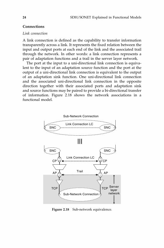
A link connection is defined as the capability to transfer informationtransparently across a link. It represents the fixed relation between theinput and output ports at each end of the link and the associated trailthrough the network. In other words: a link connection represents apair of adaptation functions and a trail in the server layer network.

The port at the input to a uni-directional link connection is equiva-lent to the input of an adaptation source function and the port at theoutput of a uni-directional link connection is equivalent to the outputof an adaptation sink function. One uni-directional link connectionand the associated uni-directional link connection in the oppositedirection together with their associated ports and adaptation sinkand source functions may be paired to provide a bi-directional transferof information. Figure 2.18 shows the network associations in afunctional model.

Serverlayer

network

CP

TCP

AP

CP

TCP

AP

Link Connection LC

Trail



SNC SNC

Link Connection LCSNC SNC

Figure 2.18 Sub-network equivalence.


Sub-network connection

A sub-network connection is defined as the capability of transferringinformation transparently across a sub-network. It is delimited byports at the boundary of the sub-network and represents the associa-tion between these ports.

Sub-network connections are generally constituted by a concaten-ation of sub-network connections and link connections. A matrix con-nection is a special case of the sub-network connection and consistsof a single (indivisible) sub-network connection. This is depicted inFigure 2.19.

Network connection

A network connection is defined as the capability of transferringinformation transparently across a layer network. It is delimited byTermination Connection Points (TCPs). It is constituted by a concate-nation of sub-network connections and/or link connections. A TCP isequivalent to the binding of the port of the trail termination to either asub-network connection or to the port of a link connection. There is noexplicit information to allow the integrity of the transferred informa-tion to be monitored. Some techniques that allow the integrity to bemonitored are described in Chapter 8. Figure 2.20 illustrates theconcatenation of a network connection. If part of a network connection

Link Connection LC


SNC

LCSNC SNCSNC

LC

SNC

Figure 2.19 Sub-network constitution.


has to be monitored, for example, because it is passing another serviceproviders domain, it is generally referred to as a tandem connection.

Chapter 7 provides a more detailed description of connectionfunctions and also contains example applications.

Trails

A trail represents the transfer of characteristic information (CI) of the clientlayer. To enable this transfer, the characteristic information will beadapted for the transport through the network between the access points(AP) and it is monitored for the performance of the transport. Two accesspoints delimit a trail, one at each end of the trail. A trail is defined as theassociation between the access points at each end of the trail. To provisiona trail, an association has to be established between the two trail termina-tions and a network connection. Figure 2.21 shows the association.

TCP

AP

TCP

AP

Tandem ConnectionLC

SNC

Network Connection

SNC SNC SNC SNCSNC

Figure 2.20 Network connection concatenation.

CP

TCP

AP

CP

TCP

AP

client layer characteristic information (CI)

Trail

Network Connection

server layer characteristic information (CI)

Figure 2.21 Trail association.


2.4.2 Transport processing functions

Initially, there were two distinct generic processing functions definedto describe the architecture of layer networks: an adaptation functionand a trail termination function. With the introduction of concatenationone more processing function was added: an interworking function.Packet based transport technologies also required an additional func-tion: a traffic conditioning function. These atomic functions are describedin the following sections.

Adaptation function

� Adaptation source function. A transport processing function thatadapts the client layer network characteristic information into aform suitable for transport over a trail in the server layer network.

� Adaptation sink function. A transport processing function thatrecovers the characteristic information of the client layer networkfrom the server layer network trail information.

� Bi-directional adaptation function. A transport processing functionthat consists of a co-located adaptation source and sink pair.

� Adaptation function I/O. Several configurations are possible:

- In the adaptation source function, one or more client layernetwork characteristic information streams are adapted into asingle adapted information stream suitable for transport over atrail in the server layer network. The adaptation sink functionprovides the inverse functionality.

This configuration is commonly used to represent the multi-plexing of several client signals into a single server signal. Theclient signals are not necessarily originating from the same layernetwork.

- In the adaptation source function a single client layer net-work characteristic information stream is split over severaloutputs and in the adaptation sink function the client infor-mation stream is reconstructed from signals present at theinputs. This configuration is used to represent inversemultiplexing.

- In the adaptation source and sink functions, the client layermay be either connection oriented or connectionless and theserver layer may also be either connection oriented or con-nectionless, see Figure 2.22 for the possible configurations.


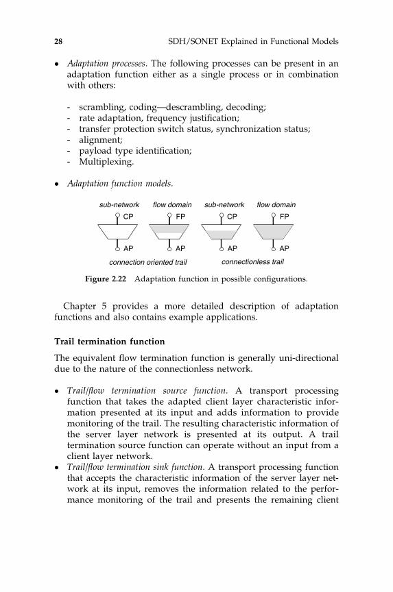
� Adaptation processes. The following processes can be present in anadaptation function either as a single process or in combinationwith others:

- scrambling, coding—descrambling, decoding;- rate adaptation, frequency justification;- transfer protection switch status, synchronization status;- alignment;- payload type identification;- Multiplexing.

� Adaptation function models.

Chapter 5 provides a more detailed description of adaptationfunctions and also contains example applications.

Trail termination function

The equivalent flow termination function is generally uni-directionaldue to the nature of the connectionless network.

� Trail/flow termination source function. A transport processingfunction that takes the adapted client layer characteristic infor-mation presented at its input and adds information to providemonitoring of the trail. The resulting characteristic information ofthe server layer network is presented at its output. A trailtermination source function can operate without an input from aclient layer network.

� Trail/flow termination sink function. A transport processing functionthat accepts the characteristic information of the server layer net-work at its input, removes the information related to the perfor-mance monitoring of the trail and presents the remaining client

CP

AP

FP

AP

CP

AP

FP

AP

connection oriented trail connectionless trail

flow domain flow domain sub-networksub-network

Figure 2.22 Adaptation function in possible configurations.


layer network information at its output. A trail termination sinkfunction can operate without an output to a client layer network.

� Bi-directional trail termination function. A transport processing func-tion that consists of a pair of co-located trail termination source andsink functions.

� Trail/flow termination function I/O. The trail/flow termination sourcefunction always has one input. There can be one or more outputspresent in a single trail/flow termination function. The singleadapted client layer network characteristic information inputstream is distributed over one or more network connections orflows in the server layer. The one input to one output configurationis used most generally. It represents the addition of the TrailOverhead to the adapted information to be transported via a singlenetwork connection or flow. The one input to multiple outputconfiguration could be used to represent inverse multiplexingwhere a single high capacity information stream is distributedover several network connections or flows each with a lowertransport capacity then the original stream.

The trail/flow termination sink function provides the inversefunctionality and has one or more inputs and single output.

� Trail/flow termination processes. The following processes may bepresent in an adaptation function either as a single process or incombination with others:

- scrambling – descrambling;- error detecting code generation – checking;- trail identification – connectivity check;- near-end and far-end performance monitoring.

� Trail/flow termination function models.

TCP

AP

TCP

AP

sub-network flow domain

connectionoriented trail

connectionlessflow

TT FT

Figure 2.23 Trail and flow termination function.


Chapter 6 provides a more detailed description of trail terminationfunctions and also contains example applications.

Interworking function

� Interworking source function, contiguous to virtual. A transport pro-cessing function that provides interworking between layer net-works with the same characteristic information but withdifferent transport structures. The function adapts a contiguousconcatenated structure into a virtual concatenated structure andvice versa. It enables the transport of the client payload overmultiple trails in a layer network that does not support theoriginal contiguous concatenated structures.

� Interworking sink function, virtual to contiguous. The transport pro-cessing function that performs the inverse of the interworkingsource function, i.e. it converts the layer network trail informationthat uses a virtual concatenated structure into the characteristicinformation of the layer network that uses a contiguous concate-nated structure.

� Interworking function I/O. The interworking source function has oneinput and multiple outputs and the interworking sink function hasmultiple inputs and a single output. The transport capability of thecontiguous concatenated structure and the virtual concatenatedstructure is exactly the same.

� Interworking processes. The following processes are present in theinterworking function:

- trail overhead distribution and reconstruction;- framing;- alignment.

� Interworking function model.

CP

CP

Figure 2.24 Interworking function.


Chapter 10 (Section 10.4) provides a more detailed description ofinterworking functions and contains an example application.

Traffic conditioning

� Traffic conditioning function. A flow processing function withthe objective to determine the conformance of incoming Ethernetframes.

� Traffic conditioning function I/O. This function is uni-directional andhas only a single input and a single output.

� Traffic conditioning processes. The complete Ethernet traffic con-ditioning process is still under study by ITU-T Studygroup 13and so what follows is a preliminary definition. The level ofconformance is expressed as one of three colors: Green, Yellow orRed. For a sequence of ingress Ethernet frames, ftj; ljgj � 0, witharrival times tj and lengths lj, the color assigned to each frameduring traffic conditioning is defined by a Bandwidth Profilealgorithm. Compliance to a Bandwidth Profile is described byfour parameters:

(1) Committed Information Rate (CIR) expressed as bits persecond. CIR must be � 0.

(2) Committed Burst Size (CBS) expressed as bytes. WhenCIR> 0, CBS must be�Maximum Ethernet frame allowedto enter the network.

(3) Excess Information Rate (EIR) expressed as bits per second.EIR must be� 0.

(4) Excess Burst Size (EBS) expressed as bytes. When EIR > 0,EBS must be�Maximum Ethernet frame allowed to enterthe network.

Two additional parameters are used to determine the beha-vior of the Bandwidth Profile algorithm. The algorithm is saidto be in color aware mode when each incoming EthernetFrame already has a level of conformance color associatedwith it and that color is taken into account in determiningthe level of conformance to the bandwidth profile parameters.The Bandwidth Profile algorithm is said to be in color blindmode when level of conformance color (if any) already asso-ciated with each incoming Ethernet Frame is ignored in deter-mining the level of conformance. Color blind mode support


is required at the UNI. Color aware mode is optional at theUNI.

- Coupling Flag (CF) must have only one of two possible values, 0or 1.

- Color Mode (CM) must have only one of two possible values,‘blind-blind’ and ‘aware-aware’.

� Traffic conditioning model.

2.4.3 Reference points

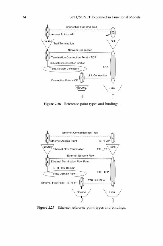
Reference points are defined as the binding between inputsand outputs of transport processing functions and/or transportentities. The allowable bindings for uni-directional and bi-directional architectures and the resulting specific types of refer-ence points are shown in Table 2.1 and are also illustrated inFigure 2.26. Note that these reference points are all concernedwith the transport of client and server layer characteristic infor-mation over the (termination) connection points ((T)CP) andserver layer adapted information over the access points (AP). InEthernet, the characteristic information consists of flows and soin general the (T)CP are referred to as (termination) flow points((T)FP).

Note that in Table 2.1 the term ‘Sub-Network Connection’ is usedfor the Sub-Network Connection function.

The equivalent Ethernet model is depicted in Figure 2.27.

uni-directionaltraffic conditioning

function

Figure 2.25 Traffic conditioning model.


Table 2.1 Allowable bindings and resulting reference points.

Architectural components

Reference

point

Adaptation

So output So input TrailTerminationFlowTermination

AP

uni-dir

Sk input Sk output uni-dir

So/Sk pair So/Sk pair bi-dir

TrailTerminationFlowTermination

So output input Sub-NetworkConnection

Flow Domain

TCP

TFP

uni-dir

Sk input output uni-dir

So/Sk pair bi-dir bi-dir

Sub-NetworkConnection

Flow Domain

input So output

Adaptation CP

uni-dir

output Sk input uni-dir

bi-dir So/Sk pair bi-dir


So output input LinkConnection

Link Flow

TCP

TFP

uni-dir

Sk input output uni-dir



So output Sk input TrailTerminationFlowTermination

TCP

TFP

uni-dir

Sk input So output uni-dir



Sk input Sk output

Adaptation

TCP

TFP

uni-dir

So output So input uni-dir

bi-dir So/Sk pair bi-dir

LinkConnection

Link Flow

output input Sub-NetworkConnection

Flow Domain

CP

FP

uni-dir

input output uni-dir

bi-dir bi-dir bi-dir

AdaptationSo input Sk output

Adaptation

CP

FP

uni-dir

Sk output So input uni-dir

So/Sk pair So/Sk pair bi-dir

AP Access Point

CP Connection Point

TCP Termination Connection Point

FP Flow Point

TFP Termination Flow Point

bi-dir bi-directional

uni-dir uni-directional

So/Sk Source/Sink


Access Point − AP

Source Sink

Source Sink

Termination Connection Point − TCP

Connection Point − CP

AP

TCP

Network Connection

Sub_Network Connection

Trail Termination

Connection Oriented Trail

Sub-network connection function

Link Connection

Figure 2.26 Reference point types and bindings.

Ethernet Access Point

Source Sink

Source Sink

Ethernet Termination Flow Point

Ethernet Flow Point − ETH_FP

ETH_AP

ETH_TFP

ETH Link Flow

Flow Domain Flow

Ethernet Connectionless Trail

Ethernet Flow Termination ETH_FT

Ethernet Network Flow

ETH Flow Domain

Figure 2.27 Ethernet reference point types and bindings.


In addition to the transport reference points the following referencepoints are also present (Table 2.2), but may not always be shown in afunctional model:

2.4.4 Components comparison

The description of the architectural components in the previoussub-sections is mainly based on ITU-T Rec. G.805 (2000). This archi-tecture is connection oriented. Occasionally, for the connectionlessarchitecture components, a reference was made to ITU-T Rec. G.809(2003). This sub-section provides a comparison of the componentsused in both architectures in Table 2.3.

It should be noted that even though the terms access group and accesspoint appear to be synonymous in both architectures, their definitionsare different:

� The access group in a connection oriented layer network is definedin terms of trail terminations, sub-networks and links; in a connec-tionless layer network it is defined in terms of flow terminations,flow domains and flow point pool links.

� The access point in a connection oriented layer network is thereference point between the adaptation and trail termination func-tion; in a connectionless layer network it is the reference pointbetween the adaptation and flow termination function. Furthermore,the connection oriented access point is associated with a trail and theconnectionless access point is associated with a connectionless trail.

This allows for a common description of a layer network for bothconnection oriented and connectionless cases.

Table 2.2 Additional reference points.

Referencepoint Name Description

MP ManagementPoint

Passes management information _MI, e.g. functionprovisioning, performance primitives, probablecauses.

TP Timing Point Passes synchronization information _TI, e.g. clock,framestart.

RP Remote Point Passes remote information _RI between associatedsink and source functions, i.e. RDI, REI.

PP ReplicationPoint

Replicates Ethernet characteristic informationETH_CI from the Ethernet adaptation sourcefunction to the Ethernet adaptation sink function.


It should be noted also that for the connection oriented layer networkboth uni-directional and bi-directional components are defined whilefor a connectionless layer network, due to its characteristics, only uni-directional components are defined. In Table 2.3, components specifiedin only one of the layer networks are indicated in bold.

2.5 CLIENT/SERVER RELATIONSHIP

The client/server relationship between adjacent layer networks is onewhere a link connection in the client layer network is supported by atrail in the server layer network as illustrated in Figure 2.28.

Table 2.3 Components of connection oriented and connectionless architecturescompared.

Connection oriented component Connectionless component

Access group Access group

Access point Access point

Adaptation Adaptation

Adaptation sink Adaptation sink

Adaptation source Adaptation source

Adapted information Adapted information

Architectural component Architectural component

Characteristic information Characteristic information

Client/server relationship Client/server relationship

Uni-directional connection Flow

Uni-directional connection point Flow point

Layer network Layer network

Link Flow point pool link

Link connection Link flow

Network connection Network flow

Sub-network Flow domain

Sub-network connection Flow domain flow

Uni-directional termination connection point Termination flow point

Topological component Topological component

Trail Connectionless trail

Trail termination Flow termination

Trail termination sink Flow termination sink

Trail termination source Flow termination source

Transport Transport

Transport entity Transport entity

Transport network Transport network

Transport processing function Transport processing function


The concept of adaptation has been introduced to describe how theclient layer network characteristic information is modified so that itcan be transported over a trail in the server layer network. Therefore,from a transport network functional viewpoint the adaptation functionfalls between the layer networks. All the reference points belonging toa single layer network can be visualized as lying on a single plane.

In the example of the client layer network only a single boundaryaccess group is shown containing only one trail termination function.The access group is bounded to the sub-network at its terminationconnection point (TCP). A TCP is connected to a connection point (CP)by a sub-network connection (SNC). The CPs are connected by linkconnections (LC). A (LC) represents the server layer trail between theaccess points (AP) at the boundary of the server layer network. (Note thatthis concept of contiguous layer boundaries in the transport networkmodel is completely different from the layering concept used in the OSIprotocol reference model described in ITU-T Rec. X.200 (1994)).

The client/server relationship can be:

� A one-to-one relationship; in this case a single client layer linkconnection is supported by a single server layer trail.

� A many-to-one relationship, generally referred to as multiplexingand described in the next section.

� A one-to-many relationship, also referred to as inverse multiplex-ing (see description in Section 2.5.2).

AP AP

CP

CP

TCP

LC

server trail

SNC

server layer

client layer

Figure 2.28 Layer network associations.


2.5.1 Multiplexing

In the many-to-one relationship, several link connections present inclient layer networks are supported by a single server layer trail at thesame time as shown in Figure 2.29.

Multiplexing techniques may be used to combine the client layersignals. The client signals may originate in different layer networks orin the same layer network, as shown in Figure 2.30.

client layer Z − CP

client Aspecific

processes

serverspecific

processes

client layer B − CP

client layer A − CP

client Bspecific

processes

client Zspecific

processes

server layer − TCP

server layer − AP

Figure 2.29 Multiplexing example.

<srv>/A_A

server layer − TCP

<srv>/B_A s<rv>/Z_A <srv>/A_A

client A = B =...= Zclient layer A = B =...= Z/ / /

Figure 2.30 Alternative representation of multiplexing.


Examples of different client layers are the Sn and Sn–Xc transportlayers and the Data Communications Network (DCN) layer. The DataCommunications Channel (DCC) provides network connectivity forthe DCN. Other general-purpose communications channels are theEngineer Order Wire (EOW) and the User Channel (USR).

The adaptation function will contain client specific processesto handle the client characteristic information present at the con-nection points and processes related to the server layer characteristicinformation.

2.5.2 Inverse multiplexing

In the one-to-many relationship, a single client layer link connection issupported by several server layer trails in parallel. Inverse multi-plexing techniques (e.g. virtual concatenation, ATM inverse multi-plexing) are used to distribute the client layer signal. The serversignals may be of the same or of different types.

The generic functional model for inverse multiplexing is depictedin Figure 2.31. The support for inverse multiplexing is realized byintroducing an inverse multiplexing sublayer. This layer consistsof an inverse multiplexing trail termination function IM_TT andan inverse multiplexing adaptation function <srv>/IM_A where<srv> represents the server layer type. The IM_TT function willprovide the trail performance monitoring of the composite signal.The <srv>/IM_A function provides the distribution and reassemblyof the composite signal over and of the n individual server layertrails. The two inverse multiplex sublayer functions and the X serverlayer network termination functions <srv>_TT can be representedby the inverse multiplexing trail termination compound functionIMc_TT.

The X server layer trails may follow different paths (diverse routing)through the network. The individual signals will have a differenttransport delay due to the differences in physical path length. The sinkside function <srv>/IM_A_Sk has to compensate this delay beforethe reassembly of the composite signal can start. The differencebetween the shortest and the longest transport delay is generallyreferred to as differential delay. The maximum acceptable differentialdelay is application and/or implementation specific. Routing theindividual signals along the same path in the network will minimizethe differential delay.


The performance of the inverse multiplex sub-layer trail is determinedby the performance of the X individual server layer trails monitored bythe <srv>_TT_Sk functions and the performance monitored by thereassembly process present in the <srv>/IM_A_Sk function. At inter-mediate monitoring points, e.g. non-intrusive monitors, only the per-formance of the X individual server layer trails is available.

If a client signal has a fixed bandwidth, the number of serverlayer trails is fixed as well. Here the layer interworking, as definedin Section 2.6, may be applicable between the single server layer trailthat supports the full client signal and the X individual server layertrails that support the inverse multiplexed client signal.

If a client signal has a variable bandwidth the number of server layertrails may vary too. The network operator, the client layer process orthe protection switching process may change the number of serverlayer trails on request. Interworking between the inverse multiplexing

IMc_TT

IM_AIIM_AP

<srv>/IM_A

. . . . . . <srv>_CI . . . . . .

IM_AI

1 2 . . . . . . X

IM_CI

IM_AP

IM_TCP

<srv>_TCP

<srv>_AP

<client>_CP

AP

AP

I_TT

<srv>TT

<srv>TT

<srv>TT

IM/<client>_A IM/<client>_A

<client>_CI <client>_CI

<srv>_TCPTCP TCPTCPTCP

<client>_CP

. . . . . . <srv>_CI . . . . . .

1 2 . . . . . . X

Figure 2.31 Inverse multiplexing.


process and the client signal adaptation process may be used toincrease the availability of the transported signal. Using as manydifferent network paths as possible will also increase the availability.

Inverse multiplexing may be used to increase the bandwidthefficiency in the transport network. This can be achieved by increasingthe number X of server trails. Figure 2.32 provides an example.

In this example, a client signal with variable bandwidth requiresfive server layer trails for its transport. Since only two separateroutes are available, three server trails are routed via route 1 andtwo trails are routed via route 2. In this case, the survivable bandwidthis two trails out of five or 40%, and the non-survivable bandwidth isthree trails out of five or 60%. By adding one extra trail and routing itvia route 2 the survivable bandwidth will become 3/5 or 60% and theunprotected bandwidth 2/5 or 40%.

2.6 LAYER NETWORK INTERWORKING

The objective of layer network interworking is to provide an end-to-end trail between different types of layer network trail terminations.

Ic_TT

I_AI

route 1

I/<client>_A

<client>_CI

Ic_TT

I_AI

I/<client>_A

<client>_CI

route 2

Figure 2.32 Bandwidth efficiency.


This requires interworking of characteristic information as differentlayer networks have by definition different characteristic information.In general, the adapted information of different layer networks for thesame client layer network is also different, although this is notnecessarily the case. Therefore, layer networking may require theinterworking of adapted information. The trail overhead of a layernetwork can be defined in terms of semantics and syntax. Providedthat the same semantics exist in the two layer networks, the trailoverhead can be interchanged by passing on the semantics from onelayer network to the other in the appropriate syntax, as defined by thecharacteristic information. In other words, layer network interworkingshall be transparent for the semantics of the trail overhead. If bothlayer networks have a different set of semantics, the layer networkinterworking is restricted to the common set of semantics. The layernetwork interworking function has to terminate (insert, supervise) thesemantics that are not interchanged.

Layer network interworking is accomplished through an inter-working processing function as depicted in Figure 2.33. The inter-working processing function supports an interworking link connectionbetween two layer network connections. The interworking link con-nection is special in the sense that it is asymmetric, delimited bydifferent types of ports. It is also special because in general it is onlytransparent for a specified set of client layers. An interworking linkis a topological component that represents a bridge between twolayer networks. The interworking link creates a ‘super layer network’,

Link Connection

Trail

SNC

SNC SNC SNC SNC

SNC

client layer

server layer X server layer Y

X< >Y

Figure 2.33 Layer network interworking.


defined by the complete set of access groups that are interworking fora specified set of client layer networks.

� Layer network interworking function, uni-directional. A transportprocessing function that converts characteristic information of onelayer network to the characteristic information of another layernetwork. The integrity of end-to-end performance and maintenanceinformation is maintained. The function may be limited to a set ofclient layer networks.

� Layer network interworking function, bi-directional. A transport proces-sing function that consists of a pair of co-located uni-directional serviceinterworking functions, one for the interworking form layer networkX to Y and the other for the interworking from layer network Y to X.

For an application of layer interworking see Chapter 10, Section 10.4.

2.7 LINKING THE FUNCTIONAL MODELAND THE INFORMATION MODEL

The main concern of utilizing the functional model methodologydescribed in this book is to provide information about the transforma-tion of payload signals and the architecture of a network or networkelement. A basic functional model is shown again in Figure 2.34. As

TT

A

TCP

TT

A

TCP

client layer trail

network connection

APAP

link connectionSNC SNC

TT

A

CP

AP

TT

A

CP

APserver layer trail

sub-network sub-network

Figure 2.34 Basic functional model entities.


described in Section 2.4.2, the adaptation function provides the cap-ability to transform the characteristic information of the client layerinto that of the server layer. The trail termination function provides theverification of the correct transport of the information. The connectionfunction provides the connectivity, i.e. sub-network connections (SNC)and link connections, within a single layer to enable the transport ofthis information between the sub-network connection points.

For the management and control of the connectivity in a sub-network,the information model methodology is used. ITU-T RecommendationsM.3100 (1995) and G.8080 (2001) describe this methodology. Just forinformation, and to enable the comparison of both models, a basicinformation model is depicted in Figure 2.35.

The following terminology is info-model specific:

� Connection Termination Point (CTP): the client side of an adaptationfunction, it represents signal state at the input/output of anadaptation function.

� Trail Termination Point (TTP): the endpoints of a network connec-tion that coincide with the ends of a trail in the functional model, itrepresents the signal state at the input/output of a trail terminationfunction.

� Sub-Network Points (SNP): a pair of addressable connection pointsin the client network between which a link connection (LC) can beestablished and, as Figure 2.35 shows, this is also recursive.

link connection (LC)

(sub) network connection (NC)

link connection (LC)SNC SNC

TTP

CTP CTP

TTP

CTP CTP

SNPSNP

SNP SNP

(sub) network

link

sub-network

Figure 2.35 Basic information model entities.


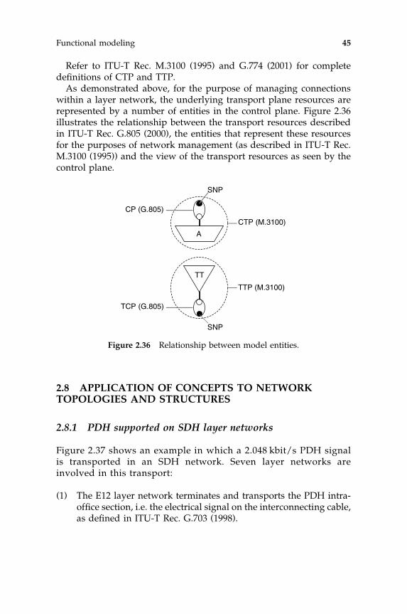
Refer to ITU-T Rec. M.3100 (1995) and G.774 (2001) for completedefinitions of CTP and TTP.

As demonstrated above, for the purpose of managing connectionswithin a layer network, the underlying transport plane resources arerepresented by a number of entities in the control plane. Figure 2.36illustrates the relationship between the transport resources describedin ITU-T Rec. G.805 (2000), the entities that represent these resourcesfor the purposes of network management (as described in ITU-T Rec.M.3100 (1995)) and the view of the transport resources as seen by thecontrol plane.

2.8 APPLICATION OF CONCEPTS TO NETWORKTOPOLOGIES AND STRUCTURES

2.8.1 PDH supported on SDH layer networks

Figure 2.37 shows an example in which a 2.048 kbit/s PDH signalis transported in an SDH network. Seven layer networks areinvolved in this transport:

(1) The E12 layer network terminates and transports the PDH intra-office section, i.e. the electrical signal on the interconnecting cable,as defined in ITU-T Rec. G.703 (1998).

TT

A

SNP

TTP (M.3100)

TCP (G.805)

CP (G.805)

CTP (M.3100)

SNP

Figure 2.36 Relationship between model entities.


(2) The P12 layer network supports the 2048 kbit/s PDH structure asdefined in ITU-T Rec. G.702 (1988).

(3) The S12 layer network supports the SDH lower-order path. Thislayer and the following are defined in ITU-T Rec. G.707 (2003).

(4) The S4 layer network supports the SDH higher-order path.(5) The MSn layer network supports the SDH multiplex section.

E12

laye

r

OSn_TCP OSn_TCP

P12_CP

S4_TT

MSn_TT

RSn_TT

OSn_TT

E12_TT

E12_TCPS12_TCP

S4_TCP

MSn_TCP

RSn_TCP

OS

n la

yer

RS

n la

yer

MS

n la

yer

S4

laye

rS

12 la

yer

S4_AP

OSn_AP

RSn_AP

MSn_AP

E12

laye

r

S12_C

S4_C

S12

trailS12_TT

S4

trail

MSn

trail

RSn

trail

S12_CP

S4_CP

MSn/S4_A

RSn/MSn_A

OSn/RSn_A

S4/S12_A

P12 layer

OSn

trail

E12_AP

S12/P12_A

S12_APE12

trail

E12/P12_A

SDH multiplexer A SDH multiplexer Zintermediate

SDH multiplexer

Figure 2.37 PDH transport over SDH network.


(6) The RSn layer network supports the SDH regenerator section.(7) The OSn SDH layer network supports the SDH optical section, i.e.

the optical signal on the interconnecting fiber.

The example shows the two SDH multiplexers, A and Z, with PDHE12 ports at the tributary side and SDH OSn ports at the SDH line side.The OSn ports are connected by a fiber or, as shown in Figure 2.37, tothe OSn ports of one (or more) intermediate SDH multiplexers thateither cross-connect the lower-order path signal S12 after terminat-ing the higher order S4 path, or cross-connect the higher-orderpath signal S4. Figure 2.37 contains all the names of the atomic func-

trail

Sn-Xv Sn-Xv

<server> network connection

network connection [X]

network connection [1]

SNC SNCSNC

SNC

AP

CP

TCP

sub-network


Sn_CI

sub-network

TCP

CP

srv srv srv srv srv srv

srv srv

Sn-X/<client> Sn-X/<client>

Figure 2.38 Example of inverse multiplexing.


tions, i.e. the termination functions <layer>_TT, the adaptation func-tion <server_layer>/<client_layer>_A and the connection function<layer>_C.

Figure 2.37 also contains the names of the reference points, i.e. theaccess points <layer>_AP, the termination connection points<layer>_TCP and the connection points <layer>_CP. The accesspoints are the end points of the trails. The S12 trail runs from nodeA to node Z, the S4 trail runs between the access points associated withthe S4_TT functions, and the MSn trails, RSn trails and OSn trails runbetween adjacent nodes.

2.8.2 Inverse multiplexing transport

Figure 2.38 shows an example of the case where the transport of aclient signal is supported through inverse multiplexing over a number(X) of parallel Sn network connections. Four layer networks are shown:

(1) the client layer network;(2) the Sn layer network providing the inverse multiplexing;(3) the first server layer, e.g. the SDH MSn/RSn/OSn layer network;(4) a second server layer, e.g. the OTN layer network;

Figure 2.38 depicts the possibility of diverse routing of inversemultiplexed signals. For example, network connection [1] is supportedby both SDH and OTN network connections and network connection[X] is supported by two consecutive SDH network connections that areconnected in an intermediate node by an Sn sub-network connection.


3

Partitioning and layering

Cutting the cake

Based on the results of the study of telecommunication networks thatexisted in 1995 and also on the fact that the new SDH and SONETtransport networks have a hierarchical structure, the model that hasbeen selected to represent a telecommunication transport network is alayered model. Partitioning is used to introduce details in a layer.

3.1 LAYERING CONCEPT

In the layered model a transport network can be represented by anumber of independent layers. Each layer in this model is used toidentify the transport of information of a specific nature. To indicatethat a specific layer is used to represent a set of connections within theoverall network, it is generally referred to as a layer network. Thehierarchical structure present in the total network means that each ofthe layer networks can use the transport capabilities of the underlyinglayer network. Therefore, a client/server relationship exists betweenadjacent layer networks in the overall network as illustrated inFigure 3.1. The definition of a particular layer network contains adescription of the generation, the transport and the termination of aspecific type of information. In the functional model this specific typeof information is referred to as characteristic information.


The layer networks that have been identified in the transportnetwork functional model should not be confused with the layersthat are used in the OSI Model (ITU-T Rec. X.200 (1994)). By definitionan OSI layer offers a specific service using one particular protocol outof a set of protocols. This is completely different from the definition ofa layer in a transport functional model where each layer networkoffers the same service, i.e. generation, transportation and termination,by using a specific protocol, i.e. the characteristic information.

Each individual layer network can be specified by a description ofits internal architectural structure. The layer network structure can bedefined according to the physical properties (e.g. connectors, fibers,cross-connects) or according to manageable properties (e.g. fixedconnections, provisionable connections). The division of a singlelayer network into the different architectural elements is generallyreferred to as partitioning. Figure 3.2 shows an example of a parti-tioned connection oriented layer network with the following architec-tural elements:

� Access groups, i.e. the input/output ports of a layer network.� Sub-networks, i.e. the provisionable connection functions provid-

ing connectivity between input and output connection points.� Links, i.e. the fixed connections used to interconnect access groups

and sub-networks.

Figure 3.2 can be used to show the partitioning of a connectionlesslayer network with the following architectural components:

� Access groups, i.e. the ingress/egress ports of a layer network.� Flow domains, i.e. the functions that transfer information between

ingress and egress flow points.

layer network d

layer network c

layer network b

client

serverlayer network a

client

server

Figure 3.1 Network layers.


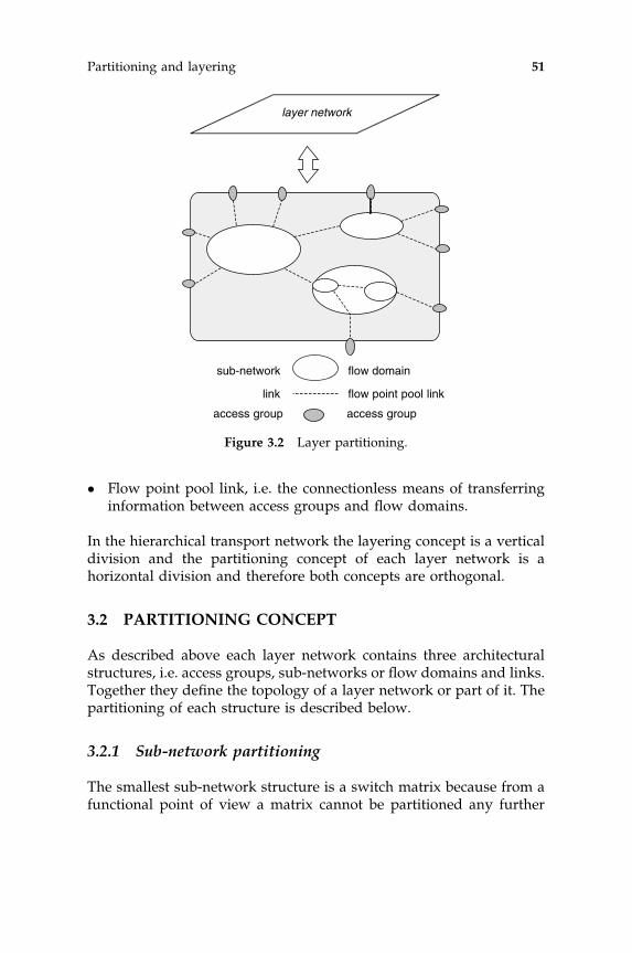
� Flow point pool link, i.e. the connectionless means of transferringinformation between access groups and flow domains.

In the hierarchical transport network the layering concept is a verticaldivision and the partitioning concept of each layer network is ahorizontal division and therefore both concepts are orthogonal.

3.2 PARTITIONING CONCEPT

As described above each layer network contains three architecturalstructures, i.e. access groups, sub-networks or flow domains and links.Together they define the topology of a layer network or part of it. Thepartitioning of each structure is described below.

3.2.1 Sub-network partitioning

The smallest sub-network structure is a switch matrix because from afunctional point of view a matrix cannot be partitioned any further

sub-network

link

layer network

access group access group

flow domain

flow point pool link

Figure 3.2 Layer partitioning.

Partitioning and layering 51

without showing implementation details. Since a model will representthe functionality of a structure and not its implementation, thesub-network is one of the elements used in the definition of a layernetwork. In a layer network the links are used to interconnectsub-networks, access groups or sub-networks and access groups. Asub-network may represent two or more contained sub-networkstogether with their related interconnecting links and is consequentlytermed a compound or containing sub-network. This representation isrecursive. The level of recursion, i.e. the level of partitioning of a sub-network, will determine the level of detail required by a specificrepresentation.

The interconnection capability provided by the ports at the bound-ary of a containing sub-network shall represent completely the con-nectivity provided by the contained sub-networks and links.

Thus the general rule for partitioning a sub-network is:

Any (containing) sub-network may be partitioned into a number ofsmaller (contained) sub-networks that are interconnected by links. Thepartitioning of a sub-network shall represent its connectivity exactly, i.e.without increasing or decreasing its interconnection capability.

An example of partitioning sub-networks is the division of a layernetwork into an international sub-network and several national sub-networks and interconnecting links. Figure 3.3 shows the containedsub-networks of a transport network extended over multiple coun-tries.

Each of these contained (inter-)national sub-networks can be parti-tioned further to provide more detail. This is illustrated in Figure 3.4where the contained sub-networks are partitioned into transit sub-networks T and access sub-networks A and interconnecting links, etc.

The layer network modeled in these figures shows all possible inputand output ports of the total network and provides a complete over-view of the total connectivity of the network. However, for certainrepresentations only a simple model is required. This is the case whenonly a single connection in the network is regarded and a one-dimensional representation will suffice. The relation between thetwo-dimensional and one-dimensional representation of the networkis depicted in Figure 3.5.

A network connection in a sub-network can be drawn in more detailby showing the contained sub-networks with their own sub-networkconnections, the interconnecting link connections and the connection


points of links and sub-networks. The termination connection pointsidentify the terminations or endpoints of a network connection. SeeFigure 3.6 for a model representation of a network connection.

The recursive nature of the partitioning concept allows the partition-ing of a network connection or a sub-network connection into a

internationalpart

nationalpart

Figure 3.3 Partitioned layer network.

AA

T

TA

Figure 3.4 Further partitioned layer network.


internationalpart

nationalpart

sub-networks

links

layer network

Figure 3.5 Layer model simplification.

CP CP CP CP

LC LCSNC SNC SNC

TCP TCP

network connection (NC)

sub-network connection (SNC) link connection (LC)

TCP termination connection pointCP connection point

Figure 3.6 Layer network connections.


concatenation of link connections and/or (contained) sub-networkswith their own sub-network connections that reflect the partitioning ofa sub-network. This is illustrated in Figure 3.7. This partitioning cancontinue until a single link connection or a matrix remains.

3.2.2 Flow domain partitioning

Generally, in a flow domain any ingress flow point can be asso-ciated with any egress flow point. Figure 3.8 shows an example

CP CP CP CP

LC LC

SNC

SNCSNC SNC

TCP TCP

network connection

CP CP CP

LC

CP

sub-network

sub-networks

SNC SNC

Figure 3.7 Recursive sub-network partitioning.

Flow Domain (FD)

(T)FP

Ingress

(T)FP

(T)FP

Egress

Ingress Egress

(T)FP

Figure 3.8 Unrestricted flow domain.


representation of a flow domain and its complete set of input andoutput (termination) flow points that provide full connectivity.

It is possible to group (termination) flow points such that theconnectivity within a part of the flow domain is limited to themembers within each group. Each group represents a fragment ofthe flow domain connectivity and is referred to as a flow domainfragment (FDFr). The relationship between a flow domain and itsfragments is illustrated in Figure 3.9.

This partitioning can be applied to any flow domain. When used in amatrix, the fragments are referred to as matrix fragments. A flowdomain fragment may be identified by its associated layer networkname, e.g. ETH_FDFr, its fragment number, e.g. FDFr_x, or by meansof grouping flow points into a characteristic fragment, e.g. in the ETHlayer network by the VLAN identifier.

A fragment of one flow domain can be associated with a fragment inanother flow domain by means of an interconnecting Flow Point Poolcomponent link or FPP link, as illustrated in Figure 3.10.

3.2.3 Link partitioning

Generally, a link in a transport network model represents one or morelink connections. A link connection is the smallest unit of manageablecapacity that is capable of transporting or routing the characteristicinformation in a specific layer network. Depending on the required

FD

(T)FP (T)FP

(T)FP(T)FP

FDFr FDFr

Figure 3.9 Flow domain partitioning.


level of detail shown in a layer network model, and to keep a modelsimple and readable, two or more links can be bundled together anddrawn as a single link. This is shown in Figure 3.11 and sometimesreferred to as parallel link partitioning.

In connectionless layer networks, parallel partitioning is also usedfor flows where a set of Flow Points (FP) is grouped in a Flow PointPool (FPP) and two FPPs are linked by an FPP link (see Figure 3.12).An ETH flow point pool link can be partitioned into ETH flow pointpool component links (cLink). There is a maximum to the number ofETH FPP cLinks within an ETH FPP link that can be supported withthe VLAN technology.

Apart from links representing parallel links, a link can also be usedin a layer network model to represent the concatenation of a link

ETH_FD

ETH_(T)FP ETH_(T)FP

ETH_(T)FP

ETH_(T)FP

ETH_(T)FP

ETH_FDFr ETH_FDFr

FPP

FPP_Link

FPP_component Link

FPP

Figure 3.10 ETH flow domain fragment connections.

n link connections

sub-networkor

access group

link / bundle

sub-networkor

access group

sub-networkor

access group

sub-networkor

access group

Figure 3.11 Parallel link partitioning.


connection, a sub-network containing a sub-network connection and alink connection. Such a link is sometimes referred to as a compoundlink or a serial partitioned link. An example is shown in Figure 3.13.

The partitioned links may themselves be recursively partitionedfurther. This partitioning can continue until a single (physical) linkconnection remains.

3.2.4 Access group partitioning

By definition an access group is a group of co-located trail terminationfunctions together with their associated access points that are con-nected to the same sub-network or link. Partitioning an access groupwill result in one or more individual trail termination functions;because these are atomic functions no further partitioning can takeplace. This is shown in Figure 3.14.

flow domainor

access group

flow domainor

access group

flow domainor

access group

flow domainor

access group

flow point component links

flow point pool link

FPP FPP

FP FP

Figure 3.12 Parallel flow partitioning.

compound link

linklink

sub-networksub-network

oraccess group

sub-networkor

access group

sub-networkor

access group

sub-networkor

access group

Figure 3.13 Serial link partitioning.


3.3 CONCEPT APPLICATIONS

3.3.1 Application of the layering concept

The layering concept applied to the transport network allows us to:

(1) Describe and identify each of the individual layer networks that ispart of an overall telecommunication network, by using a similarset of functions.

(2) Define, operate and manage each of the individual layer networksindependently of any other layer network.

(3) Assign to each individual layer network its own specific Opera-tions, Administration and Maintenance (OA&M) capabilities, e.g.performance monitoring and automatic failure recovery.

(4) Add, remove or modify each of the individual layer networkswithout affecting any of the other layer network from an archi-tectural point of view.

(5) Model telecommunication networks that contain multiple trans-port technologies in a clear and uncomplicated way.

3.3.2 Application of the partitioning concept

The partitioning concept is important as a framework for defining andidentifying:

(1) The actual or the functional network structure within each of thelayer networks that constitute the overall telecommunicationstransport network.

(2) The administrative boundaries between sub-networks managedby individual network operators. The complete set of sub-networks will provide all the possible connections within a singlelayer network. In the ideal case this could be a global layernetwork.

Figure 3.14 Access group partitioning.


(3) The boundaries determined by the proportional division anddistribution of the performance objectives among the architec-tural components of a layer network, or sub-network, that isunder the responsibility of a single network operator.

(4) The boundaries of the routing domain within a layer network thatis owned by a single network operator.

(5) The boundaries of the routing domain within a layer network, orsub-network, that is under the control of a third party (e.g.customer network management).


4

Expansion and reduction

More or less detailed

Similar to the partitioning of a network layer in order to provide moredetail by introducing sub-networks, it is also possible to partition, orexpand, an atomic function if more detail is required. This expansioncould be required to support the explanation or description of certaindetailed aspects of a functional model. Expansion can also be used toincrease the functionality provided in the network by inserting a newsublayer. In fact expansion is a method to decompose a layered network.In this way fault recovery and monitoring arrangements can bedepicted.

Conversely, if the level of detail is such that it distracts from theobjective of a provided functional model, two or more atomic functionscan be combined and represented by a compound function that willprovide the same functionality. Compound functions will also help toreduce the complexity of a model.

4.1 EXPANSION OF LAYER NETWORKS

In a telecommunications network, two specific types of layer networkscan be distinguished:

� A path layer network that is independent of the transmis-sion media and dedicated to the transfer of characteristic


information between path layer network access points at itsboundary.

� A transmission media layer network that may be media dependentand that is dedicated to the transfer of information betweentransmission media layer network access points at its boundary.A transmission media layer network will support of one or more‘path layer networks’.

The expansion of these layer networks is described in the followingsection.

4.1.1 Expansion of the path layer network

It is possible to identify in the total path layer network a set of specificpath layer networks that are likely to be managed independently by anetwork operator. Each specific path layer network of the set has itscharacteristic information transfer capability. This capability can beused either to support the transport of various types of services orsupport other specific path layer networks as clients. A specific pathlayer network can have either the transmission media layer network orother specific path layer networks as servers. The actual expansionused to generate the set of specific path layer networks is technologydependent. Each specific path layer network can have a topologyindependent of other layer networks and it should be an objective thatpaths across a specific path layer network can be set up independentlyfrom the setup of paths in other specific path layer networks. Exam-ples of the decomposition of the path layer network are given inChapter 11.

4.1.2 Expansion of the transmission media layer

It is possible to identify in the overall transmission media layernetwork a set of specific transmission media layer networks that arelikely to be managed independently by a network operator. Theconnectivity present in a transmission media layer network cannotbe modified directly by management action but most likely willrequire a physical action. This is based on the current state oftechnology; in the future it may be possible that the connectivity in a


transmission media layer network will become provisionable. Trans-mission media layer networks can be sub-divided into section layernetworks and physical media layer networks.

The section layer networks contain all the functions required for thetransfer of characteristic information between physical locations inpath layer networks. The section layer network may be expandedinto specific section layer networks as described in the examples inChapter 11.

The physical media layer networks consist of the actual opticalfibers, metallic wires or radio frequency channels to serve a sectionlayer network. The physical media layer network may be expandedinto specific physical media layer networks to represent, for exam-ple, wave division multiplexing. Since the physical media layernetwork is generally considered to be the lowest layer network, itdoes not have a server layer network. Hence a physical media layernetwork connection is supported directly by the media and not bya server trail.

4.1.3 Expansion of specific layer networks into sublayers

Sometimes it is useful to show more functional details in a specificlayer network. This can be achieved by introducing sublayers thatsupport specific transport processing functions so that reference pointscan be shown. A sublayer can be created by expanding the trailtermination functions or connection points of a specific layer network.

A sublayer is an integral part of a specific layer network. Thedifference between a sublayer and a specific layer network is thatthe functionality provided by a sublayer is neither visible to the clientlayer network nor to the server layer network of the associatedencapsulating specific layer network. A sublayer offers no transportservice to a client layer network.

Examples of expansion into sublayers are:

� trail protection schemes by the expansion of the trail termination(see Chapter 9, Section 9.2.1);

� sub-network connection protection schemes by the expansion of theconnection point (see Chapter 9, Section 9.2.2);

� tandem connection sublayers to monitor a part of a trail by theexpansion of the connection point (see Chapter 8, Section 8.3.2).

Expansion and reduction 63

The expansion of the trail termination function and connection point isillustrated in the next section.

Sublayering may be used recursively.

4.2 GENERAL PRINCIPLES OF EXPANSION OF LAYERS

It is possible to expand a layer network by expanding either thetrail terminations or the (termination) connection points of the layernetwork. Also, the adaptation functions between two adjacent layernetworks can be expanded to create a new layer network.

4.2.1 Adaptation expansion

This technique allows specifying the adaptation of the <client>characteristic information to the <server> characteristic inform-ation in more detail. It can be depicted by introducing an extra<server0> layer with its particular <server0>_TT and <server0>/<client>_A functions, shown as shaded in Figure 4.1.

<server'>_TT

<server'>/<server>_A

<server'>/<client>_A

<server'>/<client>_A

<server'>_CP

<server'>_AP

serv

er' l

ayer

Figure 4.1 Adaptation function expansion.


4.2.2 Trail termination expansion

This technique allows specifying the termination of the <client>characteristic information in more detail. It can be depicted byintroducing an extra <server0> layer with its particular <server0>/<client>_A and <server0>_TT functions, shown as shaded inFigure 4.2.

4.2.3 Connection point expansion

This technique allows the introduction of additional resources. It canbe depicted by introducing an extra <server> layer with its particular<server>/<client>_A and <server>_TT functions, shown as shadedin Figure 4.3.

<server'>/<client>_A<client>_TT

<server'>_TT

<client>_TT

<server'>_CP

<server'>_CP

serv

er' l

ayer

Figure 4.2 Trail termination function expansion.


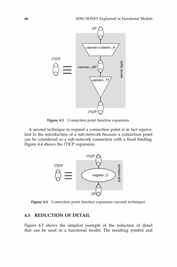
A second technique to expand a connection point is in fact equiva-lent to the introduction of a sub-network because a connection pointcan be considered as a sub-network connection with a fixed binding.Figure 4.4 shows the (T)CP expansion.

4.3 REDUCTION OF DETAIL

Figure 4.5 shows the simplest example of the reduction of detailthat can be used in a functional model. The resulting symbol and

<server>/<client>_A

<server>_TT

<server>_AP

serv

er la

yer(T)CP

CP

(T)CP

Figure 4.3 Connection point function expansion.

<signal>_C

sub-

netw

ork(T)CP

(T)CP

CP

Figure 4.4 Connection point function expansion (second technique).


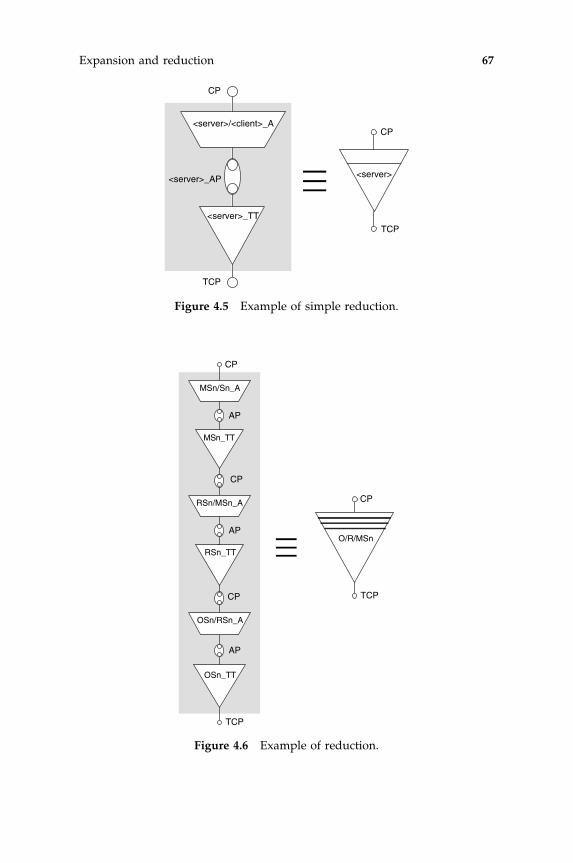
<server>/<client>_A

<server>_TT

<server>_AP

CP

TCP

TCP

CP

<server>

Figure 4.5 Example of simple reduction.

CP

MSn/Sn_A

MSn_TT

RSn/MSn_A

RSn_TT

OSn/RSn_A

OSn_TT

CP

CP

CP

TCP

AP

AP

AP

TCP

O/R/MSn

Figure 4.6 Example of reduction.


functionality is commonly referred to as a compound function. In thiscase the access point is normally a fixed binding and the sequenceof adaptation function <server>/<client>_A, access point AP andtermination function <server>_TT can be depicted by using a<server>_T compound function.

Figure 4.6 shows another example of a reduction of detail that canbe used in a functional model. Here the connection points are alsofixed bindings and the sequence of adaptation function MSn/Sn_Aand termination function MSn_TT in the multiplex section layer, theRsn/MSn_A and RSn_TT functions in the regenerator section layerand the OSn/RSn_A and Osn_TT functions in the optical section layercan be replaced by an O/R/MSn compound function.


5

Adaptation functions

The glue between layer networks

This chapter describes the generic atomic model that represents the adapta-tion of client layer network signals for transport over server layer networks.Hence it is termed an adaptation function. Although the generic model isfairly simple the level of detail in the atomic function can be raised byapplying the partitioning methodology described in Chapter 4, Section4.2.1. Examples of existing adaptation models are provided to exercise theapplication of adaptation functions.

5.1 GENERIC ADAPTATION FUNCTION

The generic adaptation function is the atomic function that performs theadaptation of a signal in a client layer network to a format that is suitablefor the transport over a trail in a server layer network. Consequently, atthe far end of the trail, this fnction will recover the original client signalfor further transport in the client layer. In the following figures,<client>represents the notation used for the client signal, e.g.MSn, Sn, OTUk, OD-Uk, etc., and<server> represents the server signal, e.g. RSn, Sn, OCh, etc.The standard convention to identify an adaptation function is:<server>/<client>_A. Figure 5.1 shows the bi-directional functional model.

In the following description of the trail termination function, the samedocumentation template is used as the template used in most of the ETSIstandardsandITU-TRecommendations. Itcontainsseparateparagraphsfor:

� symbol, a figure representing the (atomic) function in a functionalmodel;


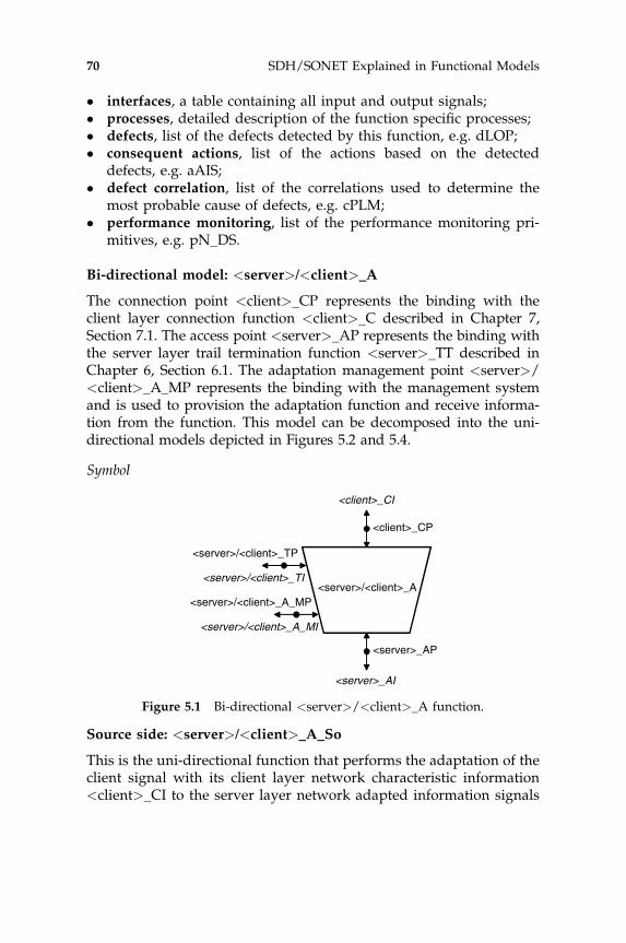
� interfaces, a table containing all input and output signals;� processes, detailed description of the function specific processes;� defects, list of the defects detected by this function, e.g. dLOP;� consequent actions, list of the actions based on the detected

defects, e.g. aAIS;� defect correlation, list of the correlations used to determine the

most probable cause of defects, e.g. cPLM;� performance monitoring, list of the performance monitoring pri-

mitives, e.g. pN_DS.

Bi-directional model: <server>/<client>_A

The connection point <client>_CP represents the binding with theclient layer connection function <client>_C described in Chapter 7,Section 7.1. The access point <server>_AP represents the binding withthe server layer trail termination function <server>_TT described inChapter 6, Section 6.1. The adaptation management point <server>/<client>_A_MP represents the binding with the management systemand is used to provision the adaptation function and receive informa-tion from the function. This model can be decomposed into the uni-directional models depicted in Figures 5.2 and 5.4.

Symbol

Source side: <server>/<client>_A_So

This is the uni-directional function that performs the adaptation of theclient signal with its client layer network characteristic information<client>_CI to the server layer network adapted information signals

<server>/<client>_A<server>/<client>_A_MP

<client>_CP

<server>_AP

<server>/<client>_A_MI

<client>_CI

<server>_AI

<server>/<client>_TP

<server>/<client>_TI

Figure 5.1 Bi-directional <server>/<client>_A function.


<server>_AI transported over the network layer trail between theserver layer network access points <server>_AP. This function islocated at the beginning or source side of the network trail.

The information flow and the processing of the <server>/<client>_A_So function are defined with reference to Figures 5.2 and 5.3.

Symbol

Interfaces

<server>/<client>_A_So

<server>/<client>_A_So_MP

<server>/<client>_RP

<client>_So_CP

<server>_So_AP

<server>/<client>_A_So_MI

<server>/<client>_RI

<client>_CI

<server>_AI



Figure 5.2 Source side <server>/<client>_A function.

<server>/<client>_A_So input and output signals.

inputs outputs

at <client>_So_CPclient signal characteristicinformation <client>_CI_nn

at <server>_So_APserver signal adaptedinformation <server>_AI_nn

at <server>/<client>_A_So_MPserver/client adaptationmanagement information<server>/<client>_A_So_MI_nn

at <server>/<client>_A_So_MPserver/client adaptationmanagement information<server>/<client>_A_So_MI_nnat <server>/<client>_RPserver/client adaptation remoteinformation<server>/<client>_RI_nn

at <server>/<client>_TPserver/client adaptation timinginformation<server>/<client>_TI_nn

Adaptation functions 71

Processes

� Activation: The <server>/<client>_A_So function shall access theaccess point when it is activated (MI_Active is true). Otherwise, itshall not access the access point and the following processes willnot be activated.

� Client data stream encoding: The client characteristic information isadapted to the server characteristic structure.

� Client alignment: The adaptation source aligns the clientdata stream with the server layer structure and adds align-ment information. While the alignment process is technologydependent, time division multiplexed (TDM) systems commonlyrequire buffering of the signal. Synchronization informationis retrieved from the timing reference point.

� Client labeling: Each client signal is ‘labeled’ to enable multi-plexing of client data streams and to identify the type of multi-plexing because the multiplexing methodology is very technologyspecific.

Defects

In general, no defects are detected by a source adaptation function.

<server>_AP

payload

<client>_CP

AI_

nnlabel

RI_nn

<ser

ver>

_RP

MI_nn

<lay

er>_

MP

PO

H

<ser

ver>

_TP

TI_nn

encode

CI_

nn

align-ment

buffer

Figure 5.3 <server>/<client>_A_S processes.


Consequent actions

In general, no consequent actions are taken by a source adaptationfunction.

Defect correlation

Since there are no defects, there is also no correlation of defects.

Performance monitoring

In general, there is no performance monitoring by a source adaptationfunction.

Sink side: <server>/<client>_A_Sk

This is the uni-directional function that performs the adaptation of theclient signal with its client layer network characteristic information<client>_CI to the server layer network adapted information signals<server>_AI transported over the network layer trail between theserver layer network access points <server>_AP. This function islocated at the end or sink side of the network trail. The informationflow and the processing of the <server>/<client>_A_Sk function aredefined with reference to Figures 5.4 and 5.5.

Symbol

<server>/<client>_A_Sk

<server>/<client>_A_Sk_MP

<server>/<client>_RP

<client>_Sk_CP

<server>_Sk_AP

<server>/<client>_A_Sk_MI

<server>/<client>_RI

<client>_CI

<server>_AI



Figure 5.4 Sink side <server>/<client>_A function.


Interfaces

<server>/<client>_A_Sk input and output signals.

inputs outputs

at <server>_Sk_APserver signal adapted informa-tion <server>_AI_nn

at <client>_Sk_CPclient signal characteristicinformation <client>_CI_nn

at <server>/<client> A_Sk_MPserver/client signal managementinformation<server>/<client>_A_Sk_MI_nn

at <server>/<client>A_Sk_MPserver/client signal managementinformation<server>/<client>_A_Sk_MI_nn

at <server>/<client>_RPserver/client adaptation remoteinformation<server>/<client>_RI_nn

at <server>/<client>_TPserver/client adaptation timinginformation<server>/<client>_TI_nn

Activate

<server>_AP

payload

<client>_CP

AI_

nn

label

RI_nn

<ser

ver>

_RP

MI_nn

<lay

er>_

MP

PO

H

<ser

ver>

_TP

TI_nn

decode

CI_

nn

align-ment

buffer

Figure 5.5 <server>/<client>_A_Sk processes.


Processes

� Activation: The <server>/<client>_A_Sk function shall access theaccess point and perform the common and specific processesoperations specified below when it is activated (MI_Active istrue). Otherwise, it shall activate the SSF signals at its output(CP) and not report its status via the management point.

� Client labeling: The recovered signal ‘label’ is used to identifycorrectly each client signal and the methodology that has to be usedto demultiplex it. This demultiplexing is very technology specific.

� Client alignment: The effect of the source alignment is removed byusing the alignment information. While the alignment process istechnology dependent, time division multiplexed (TDM) systemscommonly require buffering of the signal. The recovered clientclock is output to the timing reference point.

� Client information decoding: The original client data stream isrecovered.

Defects

Definitions of defect processing are generally not part of the functionalspecification but described in a separate document, e.g. in ITU-T Rec.G.806 (2004) clause 6.2. Defects are identified by an abbreviationprefixed with a ‘d’: dXXX, e.g. dLOP.

Consequent actions

Definitions of consequent actions are generally not part of thefunctional specification but described in a separate document, e.g.in ITU-T Rec. G.806 (2004) clause 6.3. Consequent actions are definedby equations containing detected layer defects. Consequent actionsare identified by an abbreviation prefixed with an ‘a’: aXXX, e.g.aSSF.

Defect correlation

Definitions of defect correlation are generally not part of thefunctional specification but described in a separate document,e.g. in ITU-T Rec. G.806 (2004) clause 6.4. Defect correlations aredefined by equations containing detected layer defects; server layerdefects and reporting can be disabled by provisioning. Defectcorrelations are used to find a probable cause and are identifiedby an abbreviation prefixed with a ‘c’: cXXX, e.g. cPLM.



In general, performance processing is not performed in an adaptationfunction. Performance primitives are identified by an abbreviationprefixed with a ‘p’: pXXX, e.g. pFCSError.

When the defects are persistent an alarm is raised and sent to thenetwork management system via the <server>/<client>_A_Sk_MPManagement Point.

5.2 ADAPTATION FUNCTION EXAMPLES

There are already many different adaptation functions defined, seeETSI standards EN300 417-1 to 417-7 and 417-9 to 417-10 and ITU-TRec. G.705 (2000) for PDH, G.783 (2004) for SDH, G.798 (2004) forOTN, I.732 (2000) for ATM, G.8021 (2004) for Ethernet and G.mplseq(2005) for MPLS. In this subsection only a very small subset isdescribed to serve as an example for new developments.

5.2.1 The Sn/Sm_A function

The first example is derived from ITU-T Rec. G.783 (2004) clause 12.3.1:the adaptation function Sn/Sm_A that adapts the SDH Sm layercharacteristic information for transport in the Sn layer.

(12.3.1) VC–n layer to VC–m layer adaptation Sn/Sm_A

The Sn/Sm_A (m¼ 11, 12, 2 or 3; n¼ 3 or 4) provides the primaryadaptation functionality between higher order VC–n and lower orderVC–m layer networks in SDH. It defines the TU pointer processing,and may be divided into three functions:

� pointer generation at the source side;� pointer interpretation at the sink side;� frequency justification at source and sink side.

The S4/S11�_A provides the SDH-SONET interworking functionalityfor the transport of lower order VC–11s (i.e. VT1.5 SPE) by a VC–4 viaTU-12 multiplexing. The � (asterix) indicates that this is a specialfunction because generically a VC–11 is multiplexed in a TU-11. Thisspecial function also defines the TU pointer processing, and may bedivided into four functions:

� adding at the source and removal at the sink of stuffing bytes;� pointer generation at the source side;


� pointer interpretation at the sink side;� frequency justification at the source and sink side.

The format for TU pointers, their roles for processing, and mappingsof VCs are described in ITU-T Rec. G.707 (2003).

The Sn/Sm_A function also acts as a source and sink for theoverhead octets H4 and C2. The symbol of the bi-directional adapta-tion model is shown in Figure 5.6.

This model can be further decomposed into the uni-directionalsource and sink models. These models are drawn in Figures 5.7 and 5.9.

(12.3.1.1) VC–n layer to VC–m layer adaptation sourceSn/Sm_A_So

The information flow and the processing of the Sn/Sm_A_So functionare defined with reference to Figures 5.7 and 5.8.

Symbol

Sn/Sm_ASn/Sm_A_MI

Sn_AI

Sm_CI

Sn_TI

Figure 5.6 Bi-directional Sn/Sm_A function.

Sn/Sm_A_SoSn/Sm_A_So_MI

Sn_AI

Sm_CI

Sn_TI

Figure 5.7 Sn/Sm_A_So function.


Interfaces

Processes

� Activation: The Sn/Sm_A_So function shall access the access pointwhen it is activated (MI_Active is true). Otherwise, it shall not accessthe access point and the following processes will not be activated.

� Assembly: The Sn/Sm_A function assembles VCs of lower order m(m¼ 11, 12, 2, 3) as TU-m into VCs of higher order n (n¼ 3 or 4). Inthe case of the S4/S11�_A_So function, 36 bytes of fixed stuff areadded to the VC–11.

Sn/Sm_A_So input and output signals.

inputs outputs

at the Sm_So_CP at the Sn_So_APSm_CI_Data Sn_AI_DataSm_CI_Clock Sn_AI_ClockSm_CI_FrameStart Sn_AI_FrameStartSm_CI_MultiFrameSync

at the Sn_So_TPSn_TI_ClockSn_TI_FrameStart

at the Sn/Sm_A_So_MPSn/Sm_A_So_MI_Active

Sn_AP

payload

Sm_CP

AI_

nn

label C2

MI_nn

Sn

/Sm

_A_S

o_M

P

PO

HSn

_TP

TI_nn

assembly

CI_

nn

pointerprocessing

buffer

Active

H4

mul

tifra

me

indi

catio

n

Figure 5.8 Sn/Sm_A_So processes.


� Pointer processing: Consists of:

- Pointer generation: the frame offset in bytes between a lowerorder VC and higher order VC is indicated by a TU pointer thatis assigned to that particular lower order VC.

- Frequency justification: Lower order VC data at the Sm_CP aresynchronized to the timing information at the Sm_TP referencepoint. The pointer processing function provides accommodationfor wander and plesiochronous offset in the received signal withrespect to the synchronous equipment timing reference. Thisfunction can be modeled as a data buffer that is being writtenwith data, timed from the received VC clock, and read by a VCclock derived from reference point Sn_TP.

� H4: A multiframe indicator is generated and placed in the H4 byteposition.

� C2: Signal label information derived directly from the adaptationfunction type is placed in the C2 byte position.The assembly and pointer processing and the use of H4 and C2 are

described in detail in ITU-T Rec. G.707 (2003).

Defects

None.

Consequent actions

The function shall perform the following consequent actions:

aAIS CI SSF

When an all-ONEs (i.e. AIS) signal is detected at the input Sm_CP, anall-ONEs (TU-AIS) signal shall be applied at the output Sn_AP within2 (multi)frames. Upon clearing of the all-ONEs signal at the Sm_CP,the all-ONEs (TU-AIS) signal shall be removed within 2 (multi)frames.

Defect correlations

None.


None.


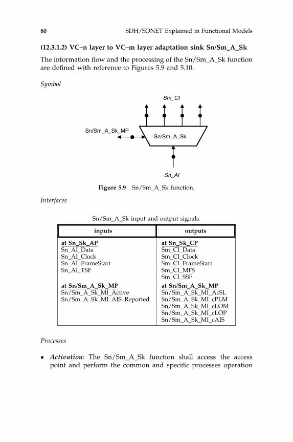
(12.3.1.2) VC–n layer to VC–m layer adaptation sink Sn/Sm_A_Sk

The information flow and the processing of the Sn/Sm_A_Sk functionare defined with reference to Figures 5.9 and 5.10.

Symbol

Interfaces

Processes

� Activation: The Sn/Sm_A_Sk function shall access the accesspoint and perform the common and specific processes operation

Sn/Sm_A_SkSn/Sm_A_Sk_MP

Sn_AI

Sm_CI

Figure 5.9 Sn/Sm_A_Sk function.

Sn/Sm_A_Sk input and output signals.

inputs outputs

at Sn_Sk_AP at Sn_Sk_CPSn_AI_Data Sm_CI_DataSn_AI_Clock Sm_CI_ClockSn_AI_FrameStart Sm_CI_FrameStartSn_AI_TSF Sm_CI_MFS

Sm_CI_SSF

at Sn/Sm_A_Sk_MP at Sn/Sm_A_Sk_MPSn/Sm_A_Sk_MI_Active Sn/Sm_A_Sk_MI_AcSLSn/Sm_A_Sk_MI_AIS_Reported Sn/Sm_A_Sk_MI_cPLM

Sn/Sm_A_Sk_MI_cLOMSn/Sm_A_Sk_MI_cLOPSn/Sm_A_Sk_MI_cAIS


specified below when it is activated (MI_Active is true). Other-wise, it shall activate the SSF signals at its output (CP) andnot report its status via the management point.

� Disassembly: The Sn/Sm_A_Sk function disassembles VC–n(n¼ 1, 3) into lower order VC–m (m¼ 11, 12, 2, 3), performingmultiframe alignment if necessary. The S4/S11�_A_Sk functionstrips off the 36 fixed stuff bytes from the VC–12 container torecover the VC–11. Note that this action may cause a discrepancybetween performance reports at an S12m_TT_Sk and an S11_TT_Skfor a VC–11 trail.

� Pointer processing: Consists of:

- Pointer interpretation: The TU pointer of each lower orderVC–m is decoded to provide information about the frameoffset in octets between the higher order VC and the indi-vidual lower order VCs.

- Frequency justification: This process must allow for conti-nuous pointer adjustments when the clock frequency of thenode where the TU was assembled is different from the local

Extract C2

Extract H4

AI_

D

AI_

TS

FC

I_S

SF

CI_

D

MI_cLOP

MI_cLOM

Sm_CP

Sn_AP

Pay

load

Sn

/Sm

_A_S

k_M

P

MI_cAIS

Def

ect

corr

elat

ions

Consequent actions

aSSF

dLOM

dPLMPO

H

aAIS

MI_cPLM

MI_AcSL

dAIS

dLOP

MI_Active

MI_cAIS_Reported

Sn

_TP

TI_nn

assembly

pointerpocessingrbuffer

Figure 5.10 Sn/Sm_A_Sk processes.


clock reference. The frequency difference between theseclocks affects the required size of the data buffer. The TUpointer interpretation is specified in ITU-T Rec. G.783 (2004)Annex A.

The pointer interpreter detects two defect conditions:

- a loss of pointer (dLOP): note that a persistent mismatchbetween provisioned and received TU type will result in a lossof pointer (dLOP) defect.

- an AIS signal in the TU (dAIS).

� C2: Byte C2 (signal label) is recovered from VC–n overhead. If amismatch is detected (dPLM) it shall be reported together with theaccepted value (AcSL) via the management reference pointSn/Sm_A_Sk_MP.

� H4: When a payload requires multiframe alignment, the H4byte contains the multiframe indicator and multiframe align-ment is performed as defined in ITU-T Rec. G.783 (2004) clause8.2.2. In this case a loss of multiframe defect (dLOM) shall bedetected.

The disassembly and pointer processing and the use of H4 and C2are described in detail in ITU-T Rec. G.707 (2003).

Defects

The defects dAIS and dLOP shall be detected in this function accord-ing to the specification in ITU-T Rec. 783 (2004) Annex A; dLOM anddPLM shall be detected in this function according to the specificationin ITU-T Rec. 806 (2004) clause 6.2.

Consequent actions

The function shall perform the following consequent actions asdescribed in ITU-T Rec. G.806 (2004) clause 6.3:for VC–3

aAIS dPLM or dAIS or dLOP

aSSF dPLM or dAIS or dLOP


for VC–11/VC–12/VC–2

aAIS dPLM or dLOM or dAIS or dLOP

aSSF dPLM or dLOM or dAIS or dLOP

Upon the declaration of aAIS, a logical all-ONEs (AIS) signal shallbe applied at the Sm_CP within 2 (multi)frames. Upon terminationof these aAIS, the all-ONEs signal shall be removed within 2 (multi)-frames.

Defect correlations

The function shall perform the following defect correlations to deter-mine the most probable fault cause as defined in ITU-T Rec. G.806(2004) clause 6.4. These fault causes shall be reported to the elementmanger via the Sn/Sm_A_Sk_MP.

cPLM dPLM and ðnot AI TSFÞ

for VC–3

cAIS dAIS and ðnot AI TSFÞ and ðnot dPLMÞ and AIS Reported

cLOP dLOP and ðnot dPLMÞ

for VC–11/VC–12/VC–2

cLOM dLOM and ðnot AI TSFÞ and ðnot dPLMÞcAIS dAIS and ðnot AI TSFÞ and ðnot dPLMÞ and ðnot dLOMÞ

and AIS Reported

cLOP dLOP and ðnot dPLMÞ and ðnot dLOMÞ


None.

5.2.2 The OCh/RSn_A function

The second example is derived from ITU-T Rec. G.798 (2004) clause12.3.5: the adaptation function OCh/RSn_A that adapts the SDH


RSn layer characteristic information for transport in the OTN OChlayer. The bi-directional representation of the function is shownin Figure 5.11.

(12.3.5) OCh to RSn adaptation (OCh/RSn_A)

The OCh to RSn adaptation functions perform the adaptation betweenthe OCh layer adapted information and the characteristic informationof a RSn layer signal.

(12.3.5.1) OCh to RSn adaptation source function (OCh/RSn_A_So)

The information flow and processing of the OCh/RSn_A_So functionare defined with reference to Figures 5.12 and 5.13.

Symbol

OCh/RSn_AOCh/RSn_A_MI

OCh_AI

RSn_CI

OCh_TI

Figure 5.11 Bi-directional Och/RSn_A function.

OCh/RSn_A_SoOCh/RSn_A_So_MI

OCh_AI

RSn_CI

Figure 5.12 Och/RSn_A_So function.


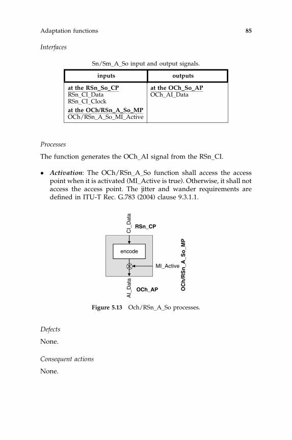
Interfaces

Processes

The function generates the OCh_AI signal from the RSn_CI.

� Activation: The OCh/RSn_A_So function shall access the accesspoint when it is activated (MI_Active is true). Otherwise, it shall notaccess the access point. The jitter and wander requirements aredefined in ITU-T Rec. G.783 (2004) clause 9.3.1.1.

Defects

None.

Consequent actions

None.

OCh_AP

RSn_CP

AI_

Dat

a

MI_Active

OC

h/R

Sn

_A_S

o_M

P

encode

CI_

Dat

a

Figure 5.13 Och/RSn_A_So processes.

Sn/Sm_A_So input and output signals.

inputs outputs

at the RSn_So_CP at the OCh_So_APRSn_CI_Data OCh_AI_DataRSn_CI_Clock

at the OCh/RSn_A_So_MPOCh/RSn_A_So_MI_Active


Defect correlations

None.


None.

(12.3.5.2) OCh to RSn adaptation sink function (OCh/RSn_A_Sk)

The information flow and processing of the OCh/RSn_A_Sk functionare defined with reference to Figures 5.14 and 5.15.

Symbol

Interfaces

OCh/RSn_A_SkOCh/RSn_A_Sk_MI

OCh_AI

RSn_CI

Figure 5.14 Och/RSn_A_Sk function.

OCh/RSn_A_Sk input and output signals.

inputs outputs

at the OCh_So_CP at the RSn_So_APOCh_CI_Data RSn_AI_DataOCh_CI_TSF RSn_AI_Clock

RSn_AI_FrameStartRSn_AI_SSF

at the Sn_So_TPSn_TI_ClockSn_TI_FrameStartat the OCh/RSn_A_So_MP at the OCh/RSn_A_Sk_MPOCh/RSn_A_Sk_MI_Active OCh/RSn_A_Sk_MI_cLOF


Processes

The processes associated with the OCh/RSn_A_Sk function aredepicted in Figure 5.15.

� Activation: The OCh/RSn_A_Sk function shall access the accesspoint and perform the common and specific processes operationspecified below when it is activated (MI_Active is true). Otherwise,it shall activate the SSF signals and generate AIS at its output (CP)and not report its status via the management point.

� Clock recovery: The function shall recover the RSn clock signalfrom the incoming data. The supported input clock range, theimmunity against the presence of consecutive identical digits, theintrinsic jitter at the STM-N output and the jitter transfer shall be asspecified in ITU-T Rec. /G.783 (2004) clause 15.1.3.

� Frame alignment: The function shall perform frame alignment on theSTM-N frame as described in ITU-T Rec. G.783 (2004) clause 8.2.1.

Defects

The defects dAIS and dLOF shall be detected in this function accord-ing to the specification in ITU-T Rec. 806 (2004) clause 6.2.

AIS detection

AI_

D

AI_

TS

FC

I_S

SF

CI_

D

MI_cLOF

RSn_CP

OCh_AP

OC

h/R

Sn_

A_S

k_M

P

Def

ect

corr

elat

ions

aSSF

aAIS

dAIS

dLOF

MI_Active

OC

h/R

Sn

_TP

TI_nn

framealignment

clockrecovery

Consequent actions

Figure 5.15 Och/RSn_A_Sk processes.


Consequent actions

The function shall perform the following consequent actions asdescribed in ITU-T Rec. G.806 (2004) clause 6.3:

aSSF AI TSF or dAIS or dLOF or ðnot MI ActiveÞaAIS AI TSF or dAIS or dLOF or ðnot MI ActiveÞ

On declaration of aAIS, the function shall output a logical all-ONEs(AIS) signal within 2 STM-N frames. On clearing of aAIS, the logicalall-ONEs (AIS) signal shall be removed within 2 STM-N frames andnormal data be output. The AIS clock start shall be independent fromthe incoming clock. The AIS clock has to be within N� 155 520 kbit/s� 20 ppm. Jitter and wander requirements are for further study.

Defect correlations

The function shall perform the following defect correlations to deter-mine the most probable fault cause as defined in ITU-T Rec. G.806(2004) clause 6.4. This fault cause shall be reported to the elementmanger via the OCh/RSn_A_Sk_MP.

cLOF dLOF and ðnot dAISÞ and ðnot AI TSFÞ

(Note: dAIS is not reported as fault cause as it is a secondary alarm andwill result in aSSF, which is reported as cSSF fault cause in theRSn_TT_Sk that directly follows this function.)


None.

5.2.3 The LCAS capable Sn–X–L/ETH_A function

The third example is derived from ITU-T Rec. G.8021 (2004) clause11.1.2: the adaptation function Sn–X–L/ETH_A that adapts the ETHlayer characteristic information for transport in an Sn–X container.This container will be transported in the VC–n layer by X individualVC–n by using LCAS capable virtual concatenation. This is a technol-ogy specific application of the model described in Chapter 10, Section10.2.5. Figure 5.16 shows the bi-directional model of this function.


The uni-directional representations of this function are depicted inFigures 5.17 and 5.19.

(11.1.2) LCAS-capable VC–n–Xv/ETH adaptation functions (Sn–X–L/ETH_A; n¼ (3, 4)

(11.1.2.1) LCAS-capable VC–n–Xv/ETH adaptation source function(Sn–X–L/ETH_A_So)

This function maps ETH_CI information onto an Sn–X–L_AI signal(n¼ 3 or 4).

The adapted information at the Sn–X–L_AP is a VC–n–X (n¼ 3 or 4),having a payload structure as described in ITU-T Rec. G.707 (2003), butwith indeterminate POH bytes: J1, B3, G1. The information flow andprocessing of the Sn–X–L/ETH_A_So function are defined with refer-ence to Figures 5.17 and 5.18.

Symbol

Sn-X-L/ETH_A

Sn-X-L/ETH_A_MI

Sn-X-L_AI

ETH_CI

Sn-X-L_TI

Sn-X-L_AI_XA

ETH_FPETH_TFP

Figure 5.16 Bi-directional Sn-X-L/ETH_A_function.

Sn-X-L/ETH_A_So

Sn-X-L/ETH_A_So_MI

Sn-X-L_AI

ETH_CI

Sn-X-L_TI

Sn-X-L_AI_XAT

ETH_PI

ETHTF_PP

ETHF_PP

ETH_TFP ETH_FP

Figure 5.17 Sn-X-L/ETH_A_So function.


Interfaces

Processes

A process diagram of this function is shown in Figure 5.18.

� Activation: The Sn–X–L/ETH_A_So function shall access theaccess point when it is activated (MI_Active is true). Otherwise, itshall not access the access point. The next three processes aredefined in ITU-T Rec. G.8021 (2004) clause 8.1.

- ‘Queuing’ process- ‘Replicate’ process- 802.3 MAC FCS generation

The next three GFP processes are defined in ITU-T Rec. G.806 (2004)clause 8.5:

� Ethernet specific GFP-F source process: In this function the GFPFCS generation is disabled (FCSenable¼ false). The UPI value

Sn–X–L/ETH_A_So input and output signals.

inputs outputs

at the ETH_TFP:ETH_CI_Data

at the ETH_FP:ETH_CI_DataETH_CI_SSF

at the Sn–X–L_AP: at the Sn–X–L_So_APSn–X–L_AI_XAT Sn_AI_Data

Sn_AI_ClockSn_AI_FrameStart

at the ETHF_PP:ETH_PI_Data

at the ETHTF_PP:ETH_PI_Data

at the Sn_So_TPSn_TI_ClockSn_TI_FrameStart

at the Sn/Sm_A_So_MPSn–X–L/ETH_A_So_MI_ActiveSn–X–L/ETH_A_So_MI_CSFEnable


‘Frame-Mapped Ethernet’ shall be inserted. The Ethernet framesare inserted into the client payload information field of the GFP-Fframes according to ITU-T Rec. G.7041 (2003) clause 7.1. Responseto ETH_CI_SSF asserted is for further study.

� Common GFP source process: The GFP channel multiplexing isnot supported (CMuxActive¼ false). The EXI value ‘0001’ shall beinserted.

� VC–n specific GFP source process: The GFP frames are mappedinto the VC–n payload area according to ITU-T Rec. G.707 (2003)clause 10.6.

� VC–n specific source process:

- C2: Signal label information is derived directly from the adapta-tion function type. The value for ‘GFP mapping’ is placed in theC2 octet position.

- H4: For the Sn–X–L/ETH_A_So function with n¼ 3, 4 the H4octet is undefined at the Sn–X–L_AP output of this function(as well as the K3, F2, F3 octets); see ITU-T Rec. G.783 (2004)clause 12.

Sn-X-L_AP

ETH_FP

AI_

Dat

a

MI_Active

Sn

-X-L

/ET

H_A

_So

_MP

queueing

CI_

Dat

a

replicate

802.3 MAC FCS

ETH specific GFP

common GFP

Sn-X-L

TI_CK

Sn

_So

_TP

ETH_TFP

CI_

Dat

a

ETH_PI_DETH_PI_D

ET

HF

_PP

ET

HT

F_P

P

TI_FS

MI_CSFEnable

C2

UPI

CI_

SS

F

AI_

FS

AI_

CK

AI_

XA

T

EXII

Sn specific GFP

Figure 5.18 Sn-X-L/ETH_A_So processes.


Defects

None.

Consequent actions

None.

Defect correlations

None.


For further study.

(11.1.2.2) LCAS-capable VC–n–Xv/ETH adaptation sink function(Sn–X–L/ETH_A_Sk)

This function extracts ETH_CI information from a VC–n-Xv serversignal (n ¼ 3 or 4), delivering ETH_CI to ETH_TFP and ETH_FP.The adapted information at the Sn–X–L_AP is a VC–n-Xv (n¼ 3or 4), having a payload structure as described in ITU-T rec. G.707(2003).

The information flow and processing of the Sn–X–L/ETH_A_Skfunction are defined with reference to Figures 5.19 and 5.20.

Symbol

Sn-X-L/ETH_A_Sk

Sn-X-L/ETH_A_Sk_MI

Sn-X-L_AI

ETH_CI

Sn-X-L_AI_XAR

ETH_PI

ETHTF_PP

ETHF_PP

ETH_TFP ETH_FP

Figure 5.19 Sn-X-L/ETH_A_Sk function.


Interfaces

Processes

In this function the signal Sn–X–L_AI_XAR is not connected to any ofthe internal processes.

� Activation: The Sn–X–L/ETH_A_Sk function shall access theaccess point and perform the common and specific processesoperation specified below when it is activated (MI_Active is true).Otherwise, it shall activate the SSF signals at its outputs (TFPand FP) and not report its status via the management point.These three processes are defined in ITU-T Rec. G.8021 (2004)clause 8.1.

- ‘Filter’ process- ‘Replicate’ process- ‘802.3 MAC frame check’ process

Sn–X–L/ETH_A_Sk input and output signals.

inputs outputs

at the Sn–X–L_AP at the ETH_TFPSn–X–L_AI_Data ETH_CI_DataSn–X–L_AI_ClocK ETH_CI_SSFSn–X–L_AI_FrameStartSn–X–L_AI_TSF at the ETH_FP:Sn–X–L_AI_XAR ETH_CI_Data

ETH_CI_SSFat the ETHF_PP:ETH_PI_Dataat the ETHTF_PP:ETH_PI_Dataat the Sn–X–L/ETH_A_Sk_MP at the Sn–X–L/ETH_A_Sk_MP:Sn–X–L/ETH_A_Sk_MI_Active Sn–X–L/ETH_A_Sk_MI_AcSL

Sn–X–L/ETH_A_Sk_MI_AcEXISn–X–L/ETH_A_Sk_MI_FilterConfig Sn–X–L/ETH_A_Sk_MI_AcUPISn–X–L/ETH_A_Sk_MI_CSF_Reported Sn–X–L/ETH_A_Sk_MI_cPLM

Sn–X–L/ETH_A_Sk_MI_cLFDSn–X–L/ETH_A_Sk_MI_cUPMSn–X–L/ETH_A_Sk_MI_cEXMSn–X–L/ETH_A_Sk_MI_cCSFSn–X–L/ETH_A_Sk_MI_pFCSError


The next three GFP processes are defined in ITU-T Rec. G.806 (2004)clause 8.5:

� Ethernet specific GFP-F sink process: This function does not sup-port GFP FCS checking (FCSdiscard¼ false), the performance pri-mitives p_FCSError and p_FD is are not used. The UPI value‘Frame-Mapped Ethernet’ shall be expected. The Ethernet framesare extracted from the client payload information field of the GFP-Fframes according to ITU-T Rec. G.7041 (2003) clause 7.1. Theaccepted UPI value AcUPI is also available at the Sn–X–L/ETH_A_Sk_MP.

� Common GFP sink process: This function does not support GFPchannel multiplexing (MI_CMuxActive¼ false). The EXI value‘0001’ shall be expected. The accepted EXI value AcEXI is alsoavailable at the Sn–X–L/ETH_A_Sk_MP.

� VC–n specific GFP sink process: The GFP frames are demappedfrom the VC–n payload area according to ITU-T Rec. G.707 (2003)clause 10.6.

Sn-X-L_AP

ETH_FP

AI_

Dat

a

MI_Active

Sn

-X-L

/ET

H_A

_Sk_

MP

filter

CI_

Dat

a

replicate

802.3 MAC FCS

ETH specific GFP

common GFP

Sn specfic GFP

Sn-X-L

ETH_TFP

CI_

Dat

a

ETH_PI_DETH_PI_DETHF_PPETHTF_PP

MI_FCSErrors

MI_AcUPI

CI_

SS

FA

I_F

S

AI_

CK

AI_

XA

R

MI_FilterConfig

CI_

SS

F

MI_cUPM

MI_AcEXIMI_cEXM

MI_cLFD

MI_AcSLMI_cPLM

AI_

TS

FMI_cCSF

C2

UPI

EXI

Figure 5.20 Sn-X-L/ETH_A_Sk processes.


� VC–n specific sink process:

- C2: The signal label is recovered from the C2 byte as per ITU-TRec. G.806 (2004) clause 6.2.4.2. The signal label value ‘GFPmapping’ shall be expected. The accepted value of the signallabel AcSL is also available at the Sn–X–L/ETH_A_Sk_MP.

Defects

The defects dPLM, dLFD, dUPM and dEXM shall be detected inthis function according to the specification in ITU-T Rec. 806 (2004)clause 6.2.

Consequent actions


aSSF AI TSF or dPLM or dLFD or dUPM or dEXM or dCSF

(Note: XAR¼ 0 results in AI_TSF being asserted in the preceding Sn–X–L_TT function, so there is no need to include it as an additionalcontributor to aSSF.)

Defect correlations

The function shall perform the following defect correlations to deter-mine the most probable fault cause as defined in ITU-T Rec. G.806(2004) clause 6.4. These fault causes shall be reported to the elementmanger via the Sn–X–L/ETH_A_Sk_MP.

cPLM dPLM and ðnot AI TSFÞcLFD dLFD and ðnot dPLMÞ and ðnot AI TSFÞcUPM dUPM and ðnot dPLMÞ and ðnot dLFDÞ and ðnot AI TSFÞcEXM dEXM and ðnot dUPMÞ and ðnot dPLMÞ and ðnot dLFDÞ

and ðnot AI TSFÞcCSF per ITU-T Rec: G:806 ð2004Þ clause 8:5:4:1:2:


The function shall perform the following performance moni-toring primitives processing. This performance monitoring


primitive shall be reported to the element manger via the Sn–X–L/ETH_ A_Sk_MP.

pFCSError count of FrameCheckSequenceErrors per second

(Note: this primitive is calculated by the MAC frame check process.)

5.2.4 GFP mapping in the Sn–X/<client>_A function

The most obvious mapping methodology that can be used to enablethe support of data transport in existing synchronous networks is theGeneric Framing Procedure (GFP) as defined in ITU-T Rec. G.7041 (2003).GFP mapping is a function of the adaptation function Sn–X/<client>_A where a packet based client signal is mapped into aconstant bitrate (CBR) signal Sn–X and X is application specific, e.g.1–256 for an SDH S4 structure. The adaptation process using GFP canbe separated into three generic parts as shown in Figure 5.21:

� one or more instances of client layer specific processes with a clientGFP part;

� common GFP processes; and� server layer specific processes with a server GFP part.

This section only describes the GFP related functionality of theadaptation function.

server/client

server_AP

client_CI

client_CP

server_AI

XA

server/client_MI

server specific processes

server specific GFP

client specific processes

client specific GFP

common GFP processes


client specific GFP


client specific GFPclient specific processes

client specific GFPclient specific processes

client specific GFP

server/client_MP

Figure 5.21 The server/client GFP adaptation function.


5.2.4.1 Source side GFP adaptation processes

Client specific GFP mapping

The client specific GFP processes perform the mapping of client datainto GFP frames. There are two types of mapping: frame-mapped GFP(GFP-F) and transparent-mapped GFP (GFP-T). Client layer specificprocesses are defined in the adaptation functions of the technologyspecific equipment recommendations.

Client specific GFP-F source processes

The inputs to this process are client frames and optionally a Signal Fail(Client_SF). The received data are processed on a frame per frame base.The output is a CBR signal consisting of GFP frames.

Client specific GFP-T source processes

The input to this process is a stream of data and control words and aLoss of Signal (Client_LOS) and Loss of Character Synchronization(Client_LCS) indication from the client layer. The received data areprocessed on a character or block of characters base. The output is aCBR signal consisting of GFP frames.

Common GFP source processes

The processes are performed on a frame per frame base. The input andthe output are CBR signals consisting of GFP frames.

Server layer specific GFP source processes

The input is a CBR signal consisting of GFP frames. Server layerspecific processes are defined in the adaptation functions of thetechnology specific equipment recommendations. For example, inthe application supporting VCAT with LCAS enabled the signal Sn–X–L_AI_XAT shall control the GFP frame rate. The output is a signalwith the server layer specific structure.

5.2.4.2 Sink side GFP adaptation processes

Client specific GFP de-mapping

The client specific GFP processes at the sink side perform thede-mapping of client data frames from GFP frames. Two types of


de-mapping, GFP-F and GFP-T, are defined. Client layer specificprocesses are defined in the adaptation functions of the technologyspecific equipment recommendations.

Client specific GFP-F sink processes

The received signal is processed on a frame per frame base. The inputconsists of GFP frames; output is the original client frame and apossible Signal Fail (Client_SF).

Client specific GFP-T sink processes

The input consists of GFP frames; the output is a stream of client dataand client control codeword octets.

Common GFP sink processes

The processes are performed on a frame per frame base. The input andoutput consist of GFP frames.

Server layer specific GFP sink processes

The input to the processes is the server layer data. Server layer specificprocesses are defined in the adaptation functions of the technologyspecific equipment recommendations. For example, in the applicationsupporting VCAT with LCAS enabled the signal Sn–X–L_AI_XAT willcontrol the GFP frame rate.


6

Trail termination functions

Or trail creation functions

This chapter describes the generic atomic model that represents thecreation and/or termination of a trail in a layer network. This is generallyreferred to as the trail termination function or abbreviated to terminationfunction. Even though the generic model is fairly simple, applying theexpansion methodology described in Chapter 4 Section 4.2.2 can raisethe level of detail in the atomic function. To clarify the application oftrail termination functions some examples of existing trail terminationmodels are provided.

6.1 GENERIC TRAIL TERMINATION FUNCTION

This atomic function is located within a layer network. The main pur-pose of this function is to monitor the integrity of the transported clientsignal and supervise its transport through the layer network. The clientsignal has been adapted for the transport by the appropriate adaptationfunction as described in Chapter 5 and is present at the access point ofa termination function. The transport entity present between two accesspoints is referred to as a trail. The information required for the monitor-ing and supervision of the adapted information may be generated andadded at the ingress and extracted and analyzed at the egress. The ter-mination source function at the ingress has the capability to create con-nectivity and performance monitoring information, generally referredto as overhead, without affecting the client or payload signal. Thetermination sink function at the egress has the capability to check the


connectivity and monitor the performance. The sink function willremove the overhead from the transported signal, i.e. the trail overheadis terminated. Depending on the technology of the layer network, theoverhead can be provided by increasing the transported capacity orusing already available, but unused, capacity.

Figure 6.1 shows the bi-directional model of a trail termination. Inthis generic model the designation <layer> has been used to identifythe technology of the layer network. When the model is used in aspecific technology the <layer> has to be replaced, for example, by Sn,MSn, ODUkP, EthP, etc.

In the following description of the trail termination function thesame documentation template is used as the template used in most ofthe ETSI standards and ITU-T Recommendations. It contains separateparagraphs for:

� symbol, a figure representing the function in a functional model;� interfaces, a table containing input and output signals;� processes, detailed description of the function specific processes;� defects, list of the defects detected by this function, e.g. dUNEQ;� consequent actions, list of the actions based on the detected

defects, e.g. aAIS;� defect correlation, list of the correlations used to determine the

most probable cause of defects, e.g. cSSF;� performance monitoring, list of the performance monitoring pri-

mitives, e.g. pN_DS.

Bi-directional model: <layer>_TT

Symbol

<layer>_TT

<layer>_TCP

<layer>_AP

<layer>_TT_MP

<layer>_CI

<layer>_AP

<layer>_TT_MI

Figure 6.1 Bi-directional <layer>_TT function.


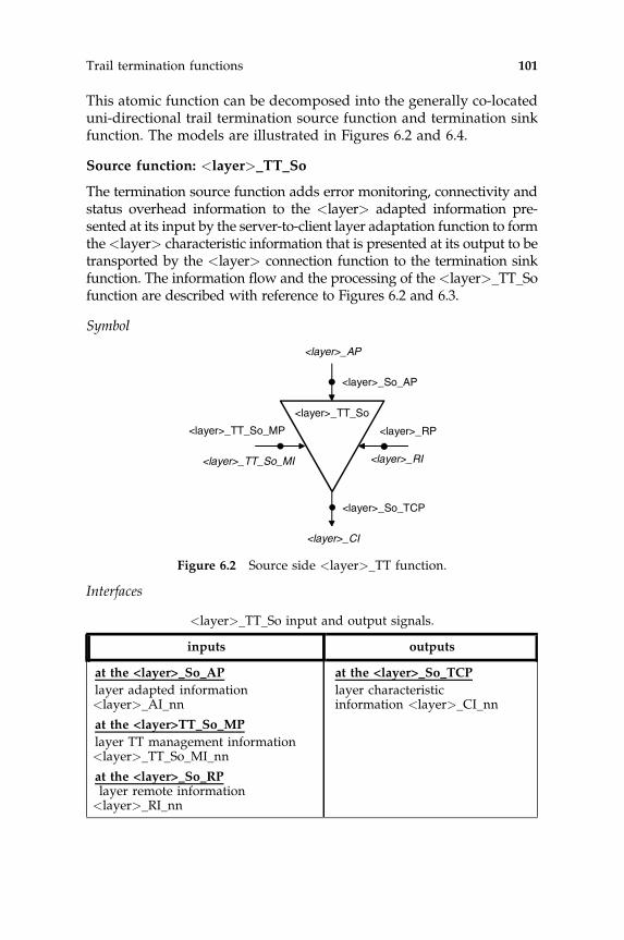
This atomic function can be decomposed into the generally co-locateduni-directional trail termination source function and termination sinkfunction. The models are illustrated in Figures 6.2 and 6.4.

Source function: <layer>_TT_So

The termination source function adds error monitoring, connectivity andstatus overhead information to the <layer> adapted information pre-sented at its input by the server-to-client layer adaptation function to formthe<layer> characteristic information that is presented at its output to betransported by the <layer> connection function to the termination sinkfunction. The information flow and the processing of the <layer>_TT_Sofunction are described with reference to Figures 6.2 and 6.3.

Symbol

Interfaces

<layer>_TT_So

<layer>_So_TCP

<layer>_So_AP

<layer>_TT_So_MP <layer>_RP

<layer>_CI

<layer>_AP

<layer>_RI<layer>_TT_So_MI

Figure 6.2 Source side <layer>_TT function.

<layer>_TT_So input and output signals.

inputs outputs

at the <layer>_So_AP at the <layer>_So_TCP

layer adapted information<layer>_AI_nn

layer characteristicinformation <layer>_CI_nn

at the <layer>TT_So_MP

layer TT management information<layer>_TT_So_MI_nn

at the <layer>_So_RPlayer remote information<layer>_RI_nn

Trail termination functions 101

Processes

The processes associated with the <layer>_TT_So function are asdepicted in Figure 6.3. Typically, there are three processes:

� provisioning and insertion of identification information to enablechecking of the connectivity in the network;

� generation and insertion of bit-interleaved parity (BIP), cyclic redun-dancy check (CRC) or frame check sequence (FCS) to enable checking ofthe integrity of the payload transport;

� returning to the far-end the status of the payload received by the asso-ciated sink function for analyzing the performance of the transport.

Defect

In general, no defects are detected by a source termination function.

Consequent actions

In general, no consequent actions are taken by a source terminationfunction.

Defect correlation

Since there are no defects there is also no correlation of defects.


In general, there is no performance monitoring by a source termina-tion function.

<layer>_TCP

payl

oad

<layer>_AP

AI_

nnC

I_nn

- error monitoring- connectivity- status infoinsertion RI_nn

<lay

er>_

RP

MI_nn

<lay

er>_

MP

PO

H

Figure 6.3 <layer>_TT_So processes.


Sink function: <layer>_TT_Sk

The termination sink function analyzes and removes the overheadinformation of the <layer> characteristic information presented to itsinput by the <layer> connection function and presents the resultingclient layer adapted information to its output for further processing bythe <layer> to client layer adaptation function. The information flowand the processing of the <layer>_TT_Sk function are described withreference to Figures 6.4 and 6.5.

Symbol

Interfaces

<layer>_TT_Sk input and output signals.

inputs outputs

at the <layer>_Sk_TCP at the <layer>_Sk_AP

layer characteristic information<layer>_CI_nn

layer adapted information<layer>_AI_nn

at the <layer>_TT_Sk_MP at the <layer>_TT_Sk_MP

layer TT management information<layer>_TT_Sk_MI_nn

layer TT management information<layer>_TT_Sk_MI_nn

at the <layer>_RPlayer remoteinformation <layer>_RI_nn

_TT_Sk

_Sk_TCP

_Sk_AP

< layer >

< layer >

< layer >

< layer >

< layer >

< layer >

< layer >

< layer >

< layer >

_TT_Sk_MP _RP

_CI

_AP

_RI_TT_Sk_MI

Figure 6.4 Sink side <layer>_TT function.


Processes

The processes associated with the <layer>_TT_Sk function are asdepicted in Figure 6.5. The error monitoring, identity and statusoverhead information is recovered to determine the status, connecti-vity and performance of the trail through the network.

Defects

Definitions of defect processing are generally not part of the functionalspecification but described in a separate document, e.g. in ITU-T Rec.G.806 (2004) clause 6.2. Defects are identified by an abbreviationprefixed with a ‘d’: dXXX, e.g. dTIM.

Consequent actions

Definitions of consequent actions are generally not part of the func-tional specification but described in a separate document, e.g. inITU-T Rec. G.806 (2004) clause 6.3. Consequent actions are definedby equations containing detected layer defects (e.g. CI_SSF), server

defectdetection

extractoverhead

information

CI_

PLD

CI_

SS

FA

I_T

SF

AI_

XX

X

AI_

D

MI_nn

<layer>_AP

<layer>_TCP

Pay

load

<lay

er>_

TT

_Sk_

MP

defe

ctco

rrel

atio

ns

Consequent actions

aXXXaTSF

dXXX

Ident.

PO

H dXXX

aAIS

aXXXRI_nn

<lay

er>_

RP

perf

orm

ance

mon

itorin

g

MI_nn

<pr

ovis

ioni

ng>

<re

port

ing>

Figure 6.5 <layer>_TT_Sk processes.


layer defects (e.g. dTIM) and can be disabled by provisioning (e.g.MI_TIMdis). Consequent actions are identified by an abbreviationprefixed with an ‘a’: aXXX, e.g. dTSF.

Defect correlation

Definitions of defect correlation are generally not part of the functionalspecification but described in a separate document, e.g. in ITU-T Rec.G.806 (2004) clause 6.4. Defect correlations are defined by equationscontaining detected layer defects, server layer defects and reportingcan be disabled by provisioning. Defects correlations are used to find aprobable cause and are identified by an abbreviation prefixed with a‘c’: cXXX, e.g. cUNEQ.


Definitions of performance processing are generally not part of thefunctional specification but described in a separate document, e.g. inITU-T Rec. G.806 (2004) clause 6.5. The number of errors and defects iscounted per second. Performance is defined by equations containingdetected layer defects, server layer defects or detected bit/block errors.Performance primitives are identified by an abbreviation prefixed witha ‘p’: pXXX, e.g. pN_DS.

6.2 TRAIL TERMINATION FUNCTION EXAMPLES

There are already many different trail termination functions defined,see ETSI standards EN300 417-1 to 417-7 and 417-9 to 417-10 and ITU-TRec. G.705 (2000) for PDH, G.783 (2004) for SDH, G.798 (2004) forOTN, I.732 (2000) for ATM, G.8021 (2004) for Ethernet and G.mplseq(2005) for MPLS. In this subsection only a subset is taken anddescribed to serve as an example for new developments.

6.2.1 The Sn_TT function

The first example is derived from ITU-T Rec. G.783 (2004) clause 12.2.1:the VC–n layer trail termination Sn_TT. In this technology the trailoverhead is transported in-band, i.e. the transported signal structurecontains octets dedicated to the overhead.


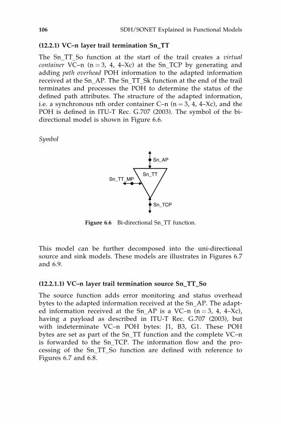
(12.2.1) VC–n layer trail termination Sn_TT

The Sn_TT_So function at the start of the trail creates a virtualcontainer VC–n (n¼ 3, 4, 4–Xc) at the Sn_TCP by generating andadding path overhead POH information to the adapted informationreceived at the Sn_AP. The Sn_TT_Sk function at the end of the trailterminates and processes the POH to determine the status of thedefined path attributes. The structure of the adapted information,i.e. a synchronous nth order container C–n (n¼ 3, 4, 4–Xc), and thePOH is defined in ITU-T Rec. G.707 (2003). The symbol of the bi-directional model is shown in Figure 6.6.

Symbol

This model can be further decomposed into the uni-directionalsource and sink models. These models are illustrates in Figures 6.7and 6.9.

(12.2.1.1) VC–n layer trail termination source Sn_TT_So

The source function adds error monitoring and status overheadbytes to the adapted information received at the Sn_AP. The adapt-ed information received at the Sn_AP is a VC–n (n ¼ 3, 4, 4–Xc),having a payload as described in ITU-T Rec. G.707 (2003), butwith indeterminate VC–n POH bytes: J1, B3, G1. These POHbytes are set as part of the Sn_TT function and the complete VC–nis forwarded to the Sn_TCP. The information flow and the pro-cessing of the Sn_TT_So function are defined with reference toFigures 6.7 and 6.8.

Sn_TT

Sn_TCP

Sn_AP

Sn_TT_MP

Figure 6.6 Bi-directional Sn_TT function.


Symbol

Interfaces

Processes

The processes associated with the Sn_TT_So function are as depictedin Figure 6.8.

� J1: The trail trace identifier (TTI) should be generated and placed inthe TTI octet position of the POH. Its value is provisioned via thereference point Sn_TT_So_MP. The format of the TTI is described inITU-T Rec. G.806 (2004) clause 6.2.2.2.

� B3: The bit interleaved parity (BIP-8) is computed over all bits of theprevious VC–n frame and placed in B3 octet position of the POH.

� G1: The performance monitoring octet. The number of remoteerrors Sn_RI_REI detected and sent by the associated sink functionis encoded in the REI position, i.e. bits 1 to 4, of the G1 octet of the

Sn_TT_So input and output signals.

inputs outputs

at the Sn_So_AP at the Sn_So_TCP

Sn_AI_DataSn_AI_ClocKSn_AI_FrameStart

Sn_CI_DataSn_CI_ClocKSn_CI_FrameStart

at the Sn_TT_So_MP

Sn_TT_So_MI_TxTI

at the Sn_So_RP

Sn_RI_RDISn_RI_REI

Sn_RPSn_TT_So

Sn_AI

Sn_So_TCP

Sn_TT_So_MI Sn_RI

Sn_So_AP

Sn_CI

Sn_TT_So_MP

Figure 6.7 Source side Sn_TT function.


POH. The REI information shall be encoded within 1ms after thedetection of the errors.

The remote defect Sn_RI_RDI detected and sent by the sink functionshall be inserted in theRDIposition, i.e. bit 5, of theG1octet in thePOH.TheRDI information shall be inserted within 1ms after the detection or clear-ing of the defect. Bits 6 and 7 of the G1 octet are reserved for the optionaluse of enhanced-RDI a SONETspecificdefect. Thedefault value is 00 or 11.

Defects

None.

Consequent actions

None.

Defect correlations

None.


None.

(12.2.1.2) VC–n layer trail termination sink Sn_TT_Sk

The sink function monitors the VC–n (n¼ (3, 4, 4–Xc)) structure receivedat the Sn_TCP for errors, and recovers the trail status from the POH. Itextracts the payload-independent overhead octets J1, B3 and G1 from theVC–n layer characteristic information to verify the connectivity and

Sn_TCP

payl

oad

Sn_APAI_Data

CI_Data

B3 calculation

J1 insertion

G1 insertionRI_RDI

RI_REI

Sn

_RP

MI_TxTI

Sn_

MP

PO

H

Figure 6.8 Sn_TT_So process.


monitor the performance of the transported trail. The VC–n is for-warded to the Sn_AP. The information flow and the processing of theSn_TT_Sk function are defined with reference to Figures 6.9 and 6.10.

Symbol

Interfaces

Sn_TT_Sk

Sn_AI

Sn_TCP

Sn_TT_Sk_MI Sn_RI

Sn_AP

Sn_CI

Sn_TT_Sk_MP Sn_RP

Figure 6.9 Sink side Sn_TT function.

Sn_TT_Sk input and output signals.

inputs outputs

at the Sn_So_TCP at the Sn_So_AP

Sn–X_CI_DataSn–X_CI_ClocKSn–X_CI_FrameStartSn–X_CI_SSF

Sn_AI_DataSn_AI_ClocKSn_AI_FrameStartSn_AI_TSFSn_AI_TSD

at the Sn_TT_Sk_MP at the Sn_TT_Sk_MP

Sn_TT_Sk_MI_TPmodeSn_TT_Sk_MI_ExTISn_TT_Sk_MI_RDI_ReportedSn_TT_Sk_MI_SSF_ReportedSn_TT_Sk_MI_DEGTHRSn_TT_Sk_MI_DEGMSn_TT_Sk_MI_EXC_XSn_TT_Sk_MI_DEG_XSn_TT_Sk_MI_1secondSn_TT_Sk_MI_TIMdisSn_TT_Sk_MI_TIMAISdis

Sn_TT_Sk_MI_AcTISn_TT_Sk_MI_cTIMSn_TT_Sk_MI_cUNEQSn_TT_Sk_MI_cEXCSn_TT_Sk_MI_cDEGSn_TT_Sk_MI_cRDISn_TT_Sk_MI_cSSFSn_TT_Sk_MI_pN_EBCSn_TT_Sk_MI_pF_EBCSn_TT_Sk_MI_pN_DSSn_TT_Sk_MI_pF_DS

at the Sn_Sk_RP

Sn_RI_RDISn_RI_REI


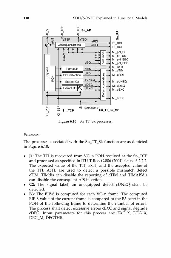
Processes

The processes associated with the Sn_TT_Sk function are as depictedin Figure 6.10.

� J1: The TTI is recovered from VC–n POH received at the Sn_TCPand processed as specified in ITU-T Rec. G.806 (2004) clause 6.2.2.2.The expected value of the TTI, ExTI, and the accepted value ofthe TTI, AcTI, are used to detect a possible mismatch defectcTIM. TIMdis can disable the reporting of cTIM and TIMAISdiscan disable the consequent AIS insertion.

� C2: The signal label; an unequipped defect cUNEQ shall bedetected.

� B3: The BIP-8 is computed for each VC–n frame. The computedBIP-8 value of the current frame is compared to the B3 octet in thePOH of the following frame to determine the number of errors.The process shall detect excessive errors cEXC and signal degradecDEG. Input parameters for this process are: EXC_X, DEG_X,DEG_M, DEGTHR.

Extract B3

Extract J1

Extract C2

RDI detection

dUNEQ

CI_

PLD

CI_

SS

FA

I_T

SF

AI_

TS

D

AI_

D

MI_pN_DS

MI_cEXCMI_cDEG

MI_cRDI

Sn_AP

Sn_TCP

Pay

load

Sn_TT_Sk_MP

MI_cSSF

Def

ectc

orre

latio

ns

Consequent actions

aTSDaTSF

ED

CV

dDEG

dTIM

dEXC

PO

H

dRDI

aAIS

aRDIaREI

RI_RDIRI_REI

Sn

_RP

perf

.mon

.

MI_pN_EBCMI_pN_EBCMI_pF_DS

MI_cUNEQ

MI_cTIMMI_AcTI

MI_<provision>

dEQ

Figure 6.10 Sn_TT_Sk processes.


� G1: The REI information shall be recovered from the G1 octetbits 1–4 and the derived performance primitives should bereported at the Sn_TT_Sk_MP. Bit 5 in the G1 octet is processedto detect the cRDI defect. The performance of the trail can bederived from the REI and RDI information and will bereported as near-end defect seconds pN_DS, far-end defectseconds pF_DS, near-end error block count pN_EBC and far-end error block count pF_EBC. To enable correlation of per-formance data in a domain, a one second timestamp ‘1 second’is distributed to all performance processes. Bits 6 and 7 of theG1 octet shall be ignored if the option enhanced-RDI is notused.

� N1: The network operator octet N1 is defined for tandem connec-tion monitoring TCM. TCM is described in Chapter 8, Section 8.3.2.The TCM specific termination function is described in ITU-T Rec.G.783 (2004) clauses 12.4.2 and 12.4.3.

� K3: Bits 5–8 are undefined and shall be ignored by this function.

If the Termination Point mode (TPmode) is true all defects andperformance data will be reported as management information(Sn_TT_Sk_MI) to the element management function.

Defects

The defects dUNEQ, dTIM, dEXC, dDEG and dRDI shall be detectedin this function according to the specification in ITU-T Rec. 806 (2004)clause 6.2. The defect dEQ represents a hardware, i.e. equipment, errorthat affects the transported signal.

Consequent actions

The function shall perform the following consequent actions asdescribed in ITU-T Rec. G.806 (2004) clause 6.3.

aAIS dUNEQ or ðdTIM and not TIMAISdisÞaRDI CI SSF or dUNEQ or dTIM

aREI ‘number of error detection code violations EDCV’

aTSF CI SSF or dUNEQ or ðdTIM and not TIMAISdisÞaTSFprot aTSF or dEXC

aTSD dDEG


On declaration of aAIS, the function shall output an all-ONEs (AIS)signal complying with the frequency limits for this signal within twoVC–n frames (250 ms). Upon termination of the above failure condi-tions, the all-ONEs shall be removed within two VC–n frames (250 ms).aRDI and aREI are reported to the far-end as remote information Sn_RIto the associated source function.

Defect correlation

The function shall perform the following defect correlations to deter-mine the most probable fault cause as defined in ITU-T Rec. G.806(2004) clause 6.4. This fault cause shall be reported to the elementmanger via the Sn_TT_Sk_MP.

cSSF CI SSF and SSF Reported and MON

cUNEQ dUNEQ and MON

cTIM dTIM and ðnot dUNEQÞ and MON

cEXC dEXC and ðnot dTIM or TIMAISdisÞ and MON

cDEG dDEG and ðnot dTIM or TIMAISdisÞ and MON

cRDI dRDI and ðnot dUNEQÞ and ðnot dTIM or TIMAISdisÞand MON and RDI Reported


The function shall perform the following performance monitoringprimitives processing see ITU-T Rec. G.806 (2004) clause 6.5. Theperformance monitoring primitives shall be reported to the elementmanagement function.

pN DS CI SSF or dUNEQ or dTIM or dEQ

pF DS dRDI

pN EBC �nN B

pF EBC �nF B

6.2.2 The OCh_TT function

The second example is derived from ITU-T Rec. G.798 (2004) clause12.2.1: the OCh layer trail termination OCh_TT. In this technology thetrail overhead is transported out-of-band, i.e. in an Optical TransportModule OTM Overhead Signal OOS.


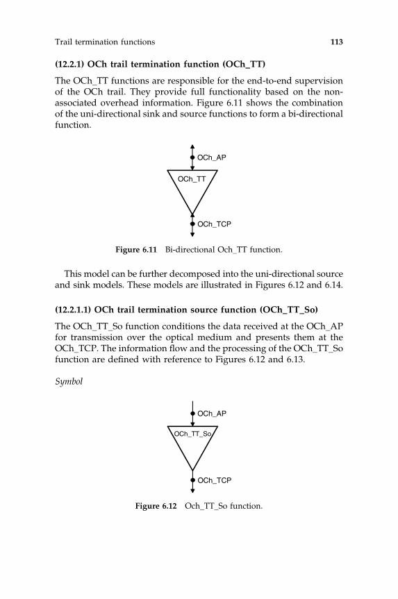
(12.2.1) OCh trail termination function (OCh_TT)

The OCh_TT functions are responsible for the end-to-end supervisionof the OCh trail. They provide full functionality based on the non-associated overhead information. Figure 6.11 shows the combinationof the uni-directional sink and source functions to form a bi-directionalfunction.

This model can be further decomposed into the uni-directional sourceand sink models. These models are illustrated in Figures 6.12 and 6.14.

(12.2.1.1) OCh trail termination source function (OCh_TT_So)

The OCh_TT_So function conditions the data received at the OCh_APfor transmission over the optical medium and presents them at theOCh_TCP. The information flow and the processing of the OCh_TT_Sofunction are defined with reference to Figures 6.12 and 6.13.

Symbol

OCh_TT

OCh_TCP

OCh_AP

Figure 6.11 Bi-directional Och_TT function.

OCh_TT_So

OCh_TCP

OCh_AP

Figure 6.12 Och_TT_So function.


Interfaces

Processes

The processes associated with the OCh_TT_So function are as depictedin Figure 6.13.

� Payload generation: The function shall generate the OCh payloadsignal (baseband signal).

Defects

None.

Consequent actions

None.

Defect correlations

None.


None.

Och_TT_So input and output signals.

input output

at the OCh_AP: at the OCh_TCP:

OCh_AI_D OCh_CI_PLD

OCh_TCP

payl

oad

gene

ratio

n

OCh_APAI_D

CI_PLD

Figure 6.13 Och_TT_So process.


(12.2.1.2) OCh trail termination sink function (OCh_TT_Sk)

The OCh_TT_Sk function recovers the OCh payload signal andreports the performance of the OCh trail. It extracts the OCh over-head (including the, FDI-P, FDI-O, and OCI signals) from theOCh signal at its OCh_TCP and detects for LOS, OCI, FDI-P andFDI-O defects. The information flow and the processing of theOCh_TT_Sk function are defined with reference to Figures 6.14and 6.15.

Symbol

Interfaces

Och_TT_Sk input and output.

inputs outputs

at the OCh_TCP: at the OCh_AP:

OCh_CI_PLDOCh_CI_OHOCh_CI_SSF-POCh_CI_SSF-O

OCh_AI_DOCh_AI_TSF-POCh_AI_TSF-O

at the OCh_TT_Sk_MP:

OCh_TT_Sk_MI_cLOS-POCh_TT_Sk_MI_cOCIOCh_TT_Sk_MI_cSSFOCh_TT_Sk_MI_cSSF-POCh_TT_Sk_MI_cSSF-O

OCh_TT_Sk

OCh_TCP

OCh_AP

OCh_TT_Sk_MP

Figure 6.14 Och_TT_Sk function.


Processes

The processes associated with the OCh_TT_So function are as depictedin Figure 6.15.

� Payload recovery: This function shall recover the OCh payloadsignal.

� LOS-P: The loss of signal; payload (OCh-LOS-P) shall be detected.� FDI-P: The forward defect indication; payload information (OCh-

FDI-P) shall be extracted from the OCh overhead of the OOS. Itshall be used for FDI-P defect detection.

� FDI-O: The forward defect indication; overhead information (OCh-FDI-O) shall be extracted from the OCh overhead of the OOS. Itshall be used for FDI-O defect detection.

� OCI: The open connection indication information (OCh-OCI) shallbe extracted from the OCh overhead of the OOS. It shall be used forOCI defect detection.

Extract FDI-O

Extract FDI-P

Extract OCI

LOS-P detection

dOCI

CI_

PLD

CI_

OH

CI_

SS

F-O

CI_

SS

F-P

AI_

TS

F-P

AI_

TS

F-O

AI_

D

MI_cLOS-P

MI_cSSF-P

MI_cSSF-O

MI_cOCI

OCh_AP

OCh_TCP

Pay

load

reco

very

OC

h_T

T_S

k_M

P

OC

hO

Hac

cess

MI_cSSF

Def

ectc

orre

latio

ns

Consequent actions

aTSF-OaTSF-P

dLO

S-P

dFD

I-P

dFD

I-O

dLOS-P

dFDI-P

dFDI-O

Figure 6.15 Och_TT_Sk processes.


Defects

The function shall detect dLOS-P, dFDI-P, dFDI-O and dOCI defects asdefined in ITU-T Rec. G.798 (2004) clause 6.2. The defect dOCI shall beset to false during CI_SSF-O and dFDI-O.

Consequent actions


aTSF-P CI SSF-P or dLOS-P or dOCI or dFDI-P

aTSF-O CI SSF-O or dFDI-O

Defect correlations

The function shall perform the following defect correlations to deter-mine the most probable fault cause. This fault cause shall be reportedto the element management function.

cLOS-P dLOS-P and ðnot dOCIÞ and ðnot FDI-PÞ and ðnot CI SSF-PÞcOCI dOCI and ðnot CI SSF-PÞ and ðnot CI SSF-OÞ

and ðnot FDI-OÞ and ðnot FDI-PÞcSSF ðCI SSF-P or dFDI-PÞ and ðCI SSF-O or dFDI-OÞ

cSSF-P ðCI SSF-P or dFDI-PÞ and ðnot cSSFÞcSSF-O ðCI SSF-O or dFDI-OÞ and ðnot cSSFÞ


For further study.

6.2.3 The ETH_FT function

The third example could have been derived from ITU-T Rec. G.8021(2004) clause 9.2. However, at the time of writing this book (April2005), this clause indicated ‘for further study’. Hence, the exampleprovided is preliminary and not complete.

This example describes the Ethernet MAC layer flow terminationfunction ETH_FT. In this technology the flow overhead is transportedpartly in-band and partly out-of-band.


(9.2) ETH flow termination function ETH_FT

The ETH_FT functions are responsible for the end-to-end supervisionof the ETH flow. They provide full functionality based on the overheadinformation. Figure 6.16 shows the bi-directional function. The ETHlayer network Characteristic Information (ETH_CI) is a (non-)contin-uous flow of ETH_CI traffic units. The ETH_CI traffic unit consists ofthe following set of signals: Destination Address (DA), Source Address(SA) and MAC Service Data Unit (M_SDU) (see ITU-T Rec. G.8010(2004) and IEEE 802.3ae (2002) clause 2). Optionally, the M_SDU mayinclude a Priority Tag (P) (see IEEE 802.1Q (2002). The ETH_CI trafficunit is transported over an ETH FPP link within a link specific frameor packet. (Note: The Preamble (PA), Start-of-Frame Delimiter (SFD)and 32-bit Frame Check Sequence (FCS) are considered part of theMAC frame (see IEEE 802.3 (2002) clause 3). In the layer networkmodel, this PA/SFD/FCS is associated with the ETH FPP link, notwith the ETH characteristic information. This modeling does notchange the requirement, in IEEE 802.1D and IEEE 802.1Q, regardingintroducing undetected frame errors.)

This model can be further decomposed into the uni-directionalsource and sink models. These models are illustrated in Figures 6.17and 6.19.

(9.2.1) Eth trail termination source function (ETH_FT_So)

The ETH_FT_So function conditions the data received at the ETH_APfor transmission over the server layer network and presents them atthe ETH_TFP. The information flow and the processing of theETH_FT_So function are defined with reference to Figures 6.17 and6.18.

ETH_FT

ETH_TCP

ETH_AP

ETH_FT_MP

Figure 6.16 Bi-directional ETH_FT function.


Symbol

Interfaces

Processes

The processes associated with the ETH_FT_So function are as depictedin Figure 6.18.

� Payload encapsulation: The function shall use the MAC protocol,defined in IEEE 802.3 (2002), to generate the ETH flow. Thisprotocol encapsulates an SDU (payload data) by adding a 14-octet header, i.e. the Protocol Control Information (PCI) (DA/SA/P), in front of the payload data octets. If the ETH FPP link uses theMAC FCS to check the integrity of the transport, the additional FCSof each ETH_CI traffic unit is generated and appended as specifiedin IEEE 802.3 (2002) subclause 4.2.4.1.2

ETH_FT_So input and output.

input output

at the ETH_AP: at the ETH_TFP:

ETH_AI_DataETH_AI_ClocK

ETH_CI_DataETH_CI_ClocK

at the ETH_FT_So_MP:

for further study

ETH_FT_So

ETH_TFP

ETH_AP

ETH_FT_So_MP

Figure 6.17 ETH_FT_ So function.


� OAM messages: Further supervisory information may be sentfrom source to sink function by OAM messages. This is for furtherstudy.

Defects

None.

Consequent actions

None.

Defect correlations

None.


None.

(9.2.2) ETH trail termination sink function (ETH_FT_Sk)

The ETH_FT_Sk function recovers the payload signal and reports theperformance of the ETH flow based on in-band and possible out-of-band information. The information flow and the processing of theETH_FT_Sk function are defined with reference to Figures 6.19 and6.20.

ETH_TFP

MA

Cpr

otoc

ol

ETH_APAI_Data

CI_Data

AI_ClocK

CI_ClocK

Figure 6.18 ETH_FT_So process.


Symbol

Interfaces

ETH_FT_Sk input and output signals.

inputs outputs

at the ETH_TFP: at the ETH_AP:

ETH_CI_DataETH_CI_ClocKETH_CI_SSF

ETH_AI_DataETH_AI_ClocKETH_AI_TSF

at the ETH_FT_Sk_MP: at the ETH_FT_Sk_MP:

for further study ETH_FT_Sk_MI_cSSFETH_FT_Sk_MI_FCSErrorsfor further study

ETH_FT_Sk

ETH_TFP

ETH_AP

ETH_FT_Sk_MP

Figure 6.19 ETH_FT_Sk function.

forfurtherstudy

CI_

Dat

a

CI_

SS

F

AI_

TS

F

AI_

Dat

a

MI_<tbd>

ETH_AP

ETH_TFP

Pay

load

reco

very

ET

H_T

T_S

k_M

P

MI_cSSF

Def

ectc

orre

latio

ns

Consequent actions

aTSF

d<tbd>

d<tbd>

Figure 6.20 ETH_FT_Sk processes.


Processes

The processes associated with the ETH_FT_So function are as depictedin Figure 6.20.

� Payload recovery: This function shall recover the SDU payloadsignal using the MAC protocol. If the ETH FPP link includes theMAC FCS, the additional FCS of each ETH_CI traffic unit ischecked as specified in IEEE 802.3 (2002) subclause 4.2.4.1.2. Iferrors are detected, the frame can be discarded. Errored framesmay be reported by MI_FCSErrors.

� OAM messages: For further study.

Defects

For further study.

Consequent actions

For further study.

Defect correlations

For further study.


For further study.


7

Connection functions

The heart of the layer network

This chapter describes the generic atomic model that represents theconnectivity in a layer network; it is generally referred to as theconnection function (or flow domain in connectionless applications).Although the generic model is fairly simple the level of detail in theatomic function can be raised by applying the partitioning methodologydescribed in Chapter 3, Section 3.2. An example of an existingconnection model is provided to exercise the application of connectionfunctions alongwith some specific applications of matrices, the mostatomic form of a connection function.

7.1 GENERIC CONNECTION FUNCTION

This is the function within a connection-oriented layer network thatprovides the capability to transfer a signal with layer specific char-acteristic information received at one of its inputs to one or more of itsoutputs. In a connectionless layer network the term connection func-tion shall be replaced by flow domain. The association between inputand outputs, i.e. connections or flows, may be provisioned from anelement or network management system. The connection function doesnot alter the information transferred from input to output. However, itmay terminate any switching protocol information and act upon it. Aconnection function only has connection points to be bound with otheratomic functions. If there are any (technology dependent) restrictions to


the connectivity, they shall be defined. In the following figures<layer> represents the notation used for the layer characteristic informa-tion <layer>_CI, e.g. Sn_CI, OTUk_CI, ODUk_ CI, ETH_CI, etc.

The standard convention to identify a connection function is<layer>_C. However, most of the time it is identified by just <layer>because the symbol identifies that it is a connection function. Note thata connection function is topologically identical to a sub-network andhas the same properties. Figure 7.1 shows the bi-directional functionalmodel of a connection function. Generally, flow domains are depicted asuni-directional models because of the uni-directional nature of flows.

Bi-directional model: <layer>_C

The connection point <layer>_TCP represents the binding with anyof the layer trail termination functions <layer>_TT described inChapter 5 and, only for the SDH S4 layer, the binding with theinterworking function described in Chapter 10, Section 10.4. Theconnection point <layer>_CP represents the binding with an adapta-tion function <server>/<layer>_A adapting the characteristic infor-mation of this layer to the server layer as described in Chapter 6. Ingeneral, the CI will consist of the data signal together with theassociated clock and framestart signals.

The connection management point <layer>_C_MP represents thebinding with the management system and is used to provision the connectionfunction and receive or retrieve information from the function.

The timing point <layer>_TP represents the binding with thetiming layer and is used to convey Timing Information (TI) such asclock and frame synchronization signals.

<layer>_C<layer>_C_MP

<layer>_TCP

<layer>_CP

<layer>_C_MI

<layer>_CI

<layer>_CI

<layer>_TP

<layer>_TI

Figure 7.1 Bi-directional <layer>_C function.


The connection function can also be depicted as a uni-directionalmodel as shown in Figure 7.2.

Uni-directional: <layer>_C

This is the uni-directional model that provides the connection of asignal with characteristic information <layer>_CI received at one ofits inputs to one or more of its outputs. The only difference with the bi-directional model is that it shows explicitly the inputs and outputs.The number of inputs and outputs towards the client layer and/or theserver layer are not necessarily the same.

Interfaces

<layer>_C<layer>_C_MP

<layer>_TCP

<layer>_CP

<layer>_C_MI

<layer>_CI

<layer>_CI

<layer>_TP

<layer>_TI

Figure 7.2 Uni-directiona l<layer>_C function.

Table 7.1 <layer>_C input and output signals.

inputs outputs

at <layer>_TCP at <layer> TCP

layer signal characteristicinformation <layer>_CI_nn

layer signal characteristicinformation <layer>_CI_nn

at <layer>_CPlayer signal characteristicinformation <layer>_CI_nn

at <layer>_CPlayer signal characteristicinformation <layer>_CI_nn

at <layer>_C_MPconnection managementinformation <layer>_C_MI_nn

at <layer>_C_MPconnection managementinformation <layer>_C_MI_nn

at <layer>_TPconnection timing information<layer>_TI_nn

Connection functions 125

Processes

The function shall be able to connect any input with any output bymeans of establishing a matrix connection between a specified inputand one or more specific outputs. It shall also be able to remove anestablished matrix connection. The network operator can provisionmatrix connections via the management interface. When the connec-tion function supports protection switching, the protection processitself can also change the matrix connections. This is described inChapter 9.

Routing

Each connection in the matrix can be provisioned by using theattributes shown in Table 7.2.

Protection

It is possible to use the connectivity provided by the matrix in theprotection schemes described in Chapter 9. However, this requires aprotection switching process that supports one or more of theseprotection schemes and specific adaptation and trail terminationfunctions in the same layer or in the server layer to provide thetriggers for the protection switch.

Defects

Not specified.

Consequent actions

On every output port this function will send a signal with theappropriate <layer>_CI structure even when there is no connection

Table 7.2 Connection provisioning.

parameter value

connection ports input/output (T)CP identifiers

connection direction – uni-directional– bi-directional

connection type – unprotected– protected (type of protection)


provisioned to any of the input ports. It is recommended, in thecharacteristic information, to send an indication that the output portis not connected; this is technology dependent. For example, in SDHand OTN the signal is labeled as ‘unequipped’ and can be identified bya structure where the signal label and path trace octets have an all-zerovalue. This ‘unequipped’ signal can be used for fault location pur-poses, e.g. identify misconnections.

Defect correlation

Not specified.


Not specified.

7.2 CONNECTION FUNCTION EXAMPLE

This section provides two examples of the connectivity capability inlayer networks:

� the connection-oriented VC–n layer connection function Sn_C;� the connectionless Ethernet flow domain ETH_FD.

7.2.1 VC–n layer connection function Sn_C

The SDH equipment recommendations ITU-T Rec. G.783 (2004) con-tain several connection functions for different layer networks. Thisexample shows only one of them: Sn_C defined in clause 12.1.1.

This is the function that transfers the VC–n signals present atits input ports to the VC–n signals at its output ports withoutaltering their structure. (Note: Neither the number of input and outputports of the connection function, nor its connectivity are specified inany of the ETSI standards or ITU-T Recommendations. These areproperties of individual network elements and are implementationdependent.)

The Sn_C connection process is a uni-directional function as illu-strated in Figures 7.3 and 7.4. The signal structure at the input andoutput ports of the function are similar, differing only in the logicalsequence of the VC–ns.


As the process does not affect the structure of the characteristicinformation, the reference points at either side of the Sn_C functionare the same, as shown in Figure 7.3. The reference points CP and TCPare identical; the latter identifies a specific binding with a trailtermination function. Figure 7.3 presents a set of atomic functions

Sn_RI

Sn_CI

1..X S

4-X

vv

S4-

Xc

Sn

Sn-XvSn-Xv_RI

SnD

SnD/Sn

SnD_RI

SnT

SnT/Sn SnT/DL

Snm SnsSns_RI

Sn_C

DL_CI

Sn-X_AI

<client>_CI

Sn_TI

S4-Xc_CI

Xx

S4_

CI

Xx

Sn_

CI

1 ....X

SnD_AI

SnT_AI

Sn_

AI

TS

F/T

SD

<server>/Sn

AP

S

Sn/<client>

<server>_AI

Sn-X/<client>

Figure 7.3a Sn layer network example; source side


that can be connected to this connection function in the VC–n layernetwork.

For a detailed description of the following atomic functions, seeITU-T Rec. G.783 (2004).

Sn_

CI 1

.

.XS

4-X

cv

S4-

Xv

Sn

Sn-Xv

SnD

SnD/Sn

SnT

SnT/SnSnT/DL

SnDmSns

Sn_C

DL_CI

Sn-X_AI

<client>_CI

S4-Xc_CI

Xx

S4_

CI

Xx

Sn_

CI

1 ....X

SnD_AI

SnT_AI

TS

F/T

SDSnTm

TS

F/T

SD

TS

F/T

SD

<server>/Sn

AP

S

SS

F/S

SD

<server>_AI

Sn_

AI

Sn/<client>

Sn-X/<client>

Figure 7.3b Sn layer network example; sink side.


Table 7.3 Atomic functions that may be connected to an Sn_C.

function description

Sn_C VC–n layer connection function

Sn_TT Sn trail termination source and sink functions

Sn–Xv_TT Sn–Xv trail termination source and sink functions

Snm_TT Sn non-intrusive monitor trail termination sink function

Sns_TT Sn supervisory-unequipped termination source and sinkfunctions

SnD_TT Sn tandem connection (option-2) termination source and sinkfunctions

SnD/Sn_A Sn tandem connection (option-2) to VC–n layer adaptationsource and sink functions

SnDm_TT Sn tandem connection (option-2) non-intrusive monitor sinkfunctions

SnT_TT Sn tandem connection (option-1) termination source and sinkfunctions

SnT/Sn_A Sn tandem connection (option-1) to VC–n layer adaptationsource and sink functions

SnTm_TT Sn tandem connection (option-1) non-intrusive monitor sinkfunction

SnT/DL_A Sn tandem connection (option-1) to data link adaptationsource and sink functions

S4–Xc> S4–Xv_I Contiguous VC–4–Xc to virtual VC–4–Xv concatenationinterworking function

S4–Xv> S4–Xc_I Virtual VC–4–Xv to contiguous VC–4–Xc concatenationinterworking function

Sn/<client>_A VC–n layer to <client> layer adaptation source and sinkfunctions, the <client> signal can be any of:

- Sm, lower order SDH VC–2, VC–12, VC–11 layer

- Pqx, PDH E31x, E32x, E4x layer

- Avp, ATM virtual path layer

- EthP, Ethernet path layer

- CBR-t, Constant bit-rate transport layer

- User channel, F2 and F3 layer

<server>/Sn_A <server> layer to VC–n layer adaptation source and sinkfunction, the <server> signal can be:

- MSn, SDH multiplex section (n¼ 1, 4, 16, 64, 256)

Note: In this example point-to-multipoint connections have to be provisioned as separate connections

to the same input (T)CP.

Note: In case a network element supports 1þ 1 protected matrix connections in its Sn_C function,

this function may contain at any moment in time either all unprotected matrix connections, or all

1þ 1 protected matrix connections, or a mixture of unprotected and 1þ 1 protected matrix

connections. The actual set of matrix connections, associated connection types and directions is an

operational parameter controlled by network management.


Symbol

The number of available inputs and outputs is normally symmetrical,i.e. p¼ q and r¼ s.

Interfaces

Sn_C

Sn_C_MP

Sn_TCP

Sn_CP

Sn_C_MI

Sn_CI

Sn_CI

Sn_TPSn_TI

p

sr

q

Figure 7.4 Uni-directional Sn_C symbol.

Table 7.4 Sn_C input and output signal.

Inputs Outputs

Per Sn_TCP and Sn_CP Per Sn_TCP and Sn_CPSn_CI_DataSn_CI_ClockSn_CI_FrameStart

Sn_CI_DataSn_CI_ClockSn_CI_FrameStart

Once per function:Sn_TI_ClockSn_TI_FrameStart

Per input and outputconnection point:Sn_C_MI_ConnectionPortIds

Per matrix connection:Sn_C_MI_ConnectionTypeSn_C_MI_Directionality

Per SNC protection group: Per SNC protection group:Sn_CI_APSSn_CI_SSFSn_CI_SSDSn_AI_TSFSn_AI_TSDSn_C_MI_PROTtypeSn_C_MI_OPERtypeSn_C_MI_WTRtimeSn_C_MI_HOtimeSn_C_MI_EXTCMD

Sn_CI_APS


Processes

In the Sn_C function, VC–n layer characteristic information is routedbetween input (termination) connection points ((T)CPs) and output(T)CPs by means of matrix connections. (T)CPs may be allocatedwithin a protection group.

Routing

The function shall be able to connect a specific input with a specificoutput by means of establishing a matrix connection between thespecified input and output. It shall be able to remove an establishedmatrix connection.

Each (matrix) connection in the Sn_C function should be character-ized by the parameters shown in Table 7.5.

Protection

If the connection function supports protection switching, additionalparameters have to be provisioned as shown in Table 7.6.

Table 7.5 Sn_Cconnection provisioning.

parameter value

Sn_C_MI_ConnectionPortIds Set of (T)CP identifiers, input, output

Sn_C_MI_ConnectionType – unprotected– 1þ 1 protected– 1:1 protected– . . .

Sn_C_MI_Directionality – uni-directional– bi-directional

Table 7.6 protection provisioning.

parameter value

Sn_C_MI_PROTtype Protection group selection, i.e. the set of connectionpoints (T)CP, the protection architecture: 1þ 1/1:n/m:n, switching type: uni-/bi-directional,operation type: APS usage: true/false, extra traffic:true/false)

Sn_C_MI_OPERtype revertivenon-revertive

Sn_C_MI_WTRtime 0–12 minutes, in steps of 1 minute


Table 7.6 (Continued)

The operation of the protection switch depends on the protectiontype and may be initiated either by signals from the layer itself, e.g.TSF and TSD, or from the server layer, e.g. SSF and SSD, by the APSprotocol from the far-end, or upon request from the operator via theelement management system.

Provided no protection switching action is activated/required, thefollowing changes to (the configuration of) a connection shall bepossible without disturbing the CI passing the connection:

� addition and removal of protection;� addition and removal of connections to/from a broadcast connec-

tion;� change between operation types;� change of Wait-To-Restore time;� change of Hold-off time.

Unequipped VC generation

The function shall generate an unequipped VC–n signal, as defined inITU-T Rec. G.707 (2003). This is a signal having an all-zero value in thehigher order virtual container path overhead signal label octet (C2),the tandem connection monitoring byte (N1) and the path trace byte(J1), and a valid BIP-8 byte (B3). The virtual container payload and theremaining path overhead bytes are unspecified.

Defects

None.

Consequent actions

If an output of this function is not connected to one of its inputs, thefunction shall connect the unequipped VC–n (with valid frame start(FS) and SSF¼ false) to the output. This may be implemented byproviding a trail termination function UNEQ_TT_So that transmits theunequipped signal and that is connected to all unused outputs.

Sn_C_MI_HOtime 0–10 seconds, in steps of 100 ms

Sn_C_MI_EXTCMD CLearRequestLockOutForcedSwitchManualSwitchEXERcise


Defect correlations

None.


None.

7.2.2 ETH flow domain

The second example is the Ethernet flow domain defined in ITU-T Rec.G.8010 (2004) clause 6.3.2.2.

The Ethernet flow domain ETH_FD is defined as the functionalitythat is available to transfer Ethernet characteristic information ETH_CIbetween a set of (termination) flow points ETH_FP and/or ETH_TFP.The association between one ingress and one or more egress ETH(termination) flow points, provisioned to transfer ETH_CI traffic unitsacross the ETH flow domain, need not be present at all times. Ingeneral, ETH flow domains may be partitioned into smaller flowdomains interconnected by ETH flow point pool links as describedin Chapter 3, Section 3.2.4. The matrix (e.g. bridge) is a special case ofan ETH flow domain.

An ETH flow domain provides broadcast connectivity between theconnected ETH (termination) flow points. An ETH_CI traffic unitreceived via an input port (e.g. A in Figure 7.5) of the ETH flow domainis forwarded to all output ports on the ETH flow domain (B, C, D), with

ETH_FDETH_(T)FPA

Ingress

ETH_(T)FPC

ETH_(T)FPD

ETH_(T)FPB

Egress

ETH_FDF

ETH_FDF

ETH_FDF

Figure 7.5 ETH flow domain connectivity.


the exception of the output port (A) that is in the same bi-directionalETH (termination) flow point as the input port.

By means of ETH network management, ETH control plane actionsand/or MAC learning, connectivity for a particular ETH flow pointcan be restricted.

7.3 CONNECTION MATRIX EXAMPLES

Generally, the connection function described in the previous sectionsis highly flexible and will provide full flexibility between its inputports and output ports as illustrated in Section 7.3.1. In general, theconnection matrix has n input ports and n output ports, i.e. it is ann� n matrix. However, due to implementation constraints the con-nectivity may be affected. Some of the limitations could be:

� Only bi-directional connections are supported: when input[i] isconnected to output[j] at the same time input [j] will be connectedto output[i].

� Only point-to-point connections are supported: when input[i] isconnected to output[j] it is not possible to connect input[i] also tooutput[k].

� Blocking in a multistage connection matrix: depending on thenumber of connections already present in the matrix it is not alwayspossible to connect input[i] with output[j].

� No connections within a group of ports: e.g. input[i] cannot beconnected to output[j] if they are both tributary ports.

� No rearrangement of the multiplex structure: if the server layeruses multiplexing for the transport of multiple client signals theorder of the client signal in the multiplex (e.g., time slots, frequencyslots, wavelength slots) cannot be interchanged, i.e. input[i] canonly be connected to output[i].

It is possible to represent the limited connectivity by grouping inputand output ports and describe the connectivity between the ports asillustrated in the following examples.

7.3.1 Connection matrix example for full connectivity

This is the most generic example of a matrix. In this matrix there are norestrictions to the connectivity. Every input port can be connected to


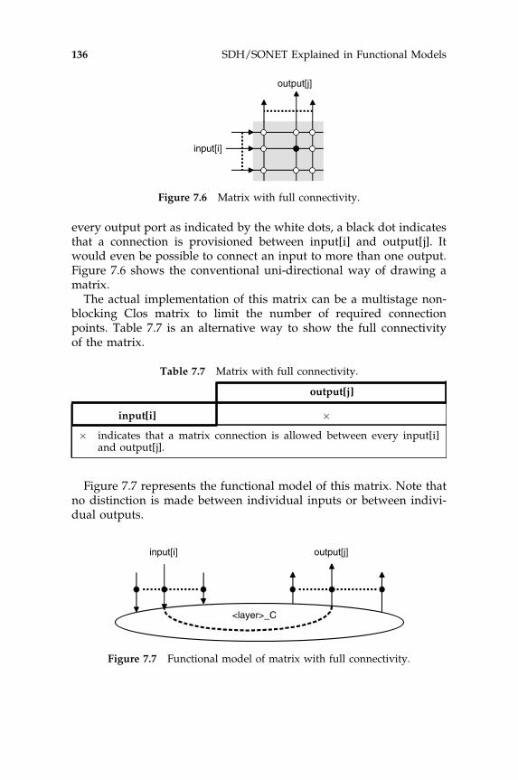
every output port as indicated by the white dots, a black dot indicatesthat a connection is provisioned between input[i] and output[j]. Itwould even be possible to connect an input to more than one output.Figure 7.6 shows the conventional uni-directional way of drawing amatrix.

The actual implementation of this matrix can be a multistage non-blocking Clos matrix to limit the number of required connectionpoints. Table 7.7 is an alternative way to show the full connectivityof the matrix.

Figure 7.7 represents the functional model of this matrix. Note thatno distinction is made between individual inputs or between indivi-dual outputs.

input[i]

output[j]

Figure 7.6 Matrix with full connectivity.

Table 7.7 Matrix with full connectivity.

output[j]

input[i] �� indicates that a matrix connection is allowed between every input[i]

and output[j].

<layer>_C

input[i] output[j]

Figure 7.7 Functional model of matrix with full connectivity.


7.3.2 Connection matrix example for two groups

In this example the total set of inputs and outputs is divided into twodistinctive groups: a line group and a tributary group. The line groupcontains the inputs and outputs of the signals that are transported overthe network and acts as the server of the client signals passing theinputs and outputs in the tributary group. Normally, this matrix onlysupports the provisioning of connections between the line group andthe tributary group and does not support connections restricted toonly the line group or tributary group. However, some implementa-tions allow loopbacks, i.e. connections provisioned between the inputand output of the same line or tributary signal. Loopbacks can betransparent where the input[i] remains connected to the originaloutput[j] as provisioned before the loopback was applied, or non-transparent where the signal at output[j] is replaced by an ‘idle’, e.g.AIS signal. Figure 7.8 illustrates this matrix with loopback capability.

Table 7.8 represents the connectivity of this matrix.

input[i]

output[j]

line

tributary

line tributary

Figure 7.8 Matrix for two groups.

Table 7.8 Connection matrix for 2 groups.

Output[j]

Line Tributary

Input[i]Line i¼ j �

Tributary � i¼ j

� Indicates matrix connection possible for any i and j.i¼ j Indicates matrix connection only possible for i¼ j (i.e. loopback).


Figure 7.9 shows the functional model of a connection matrix fortwo groups with an example bi-directional connection from line[i] totributary[j] and Figure 7.10 shows a transparent line loopback forline[i] connected to tributary[j].

7.3.3 Connection matrix example for three groups

In this example the total set of inputs and outputs is divided into threegroups, each group containing both inputs and outputs. Generally, thematrix provided here is present in network elements that are part of anetwork with a ring structure. To make a distinction between the linesthat connect to the two adjacent network elements they are identifiedas ‘line west’ and ‘line east’. Since not all signals received at the lineside are terminated locally but are passed through the tributary,signals are generally referred to as add/drop signals. The networkelement is referred to as an Add/Drop Multiplexer ADM. An example ofa ring topology with four ADMs is depicted in Figure 7.11.

<layer>_C

P[j] P[j]

P[i] P[i]

tributary side

line side

Figure 7.9 Matrix for two groups with bi-directional connection.

<layer>_C

P[j] P[j]

P[i] P[i]

tributary side

line side

Figure 7.10 Matrix for two groups with loopback.


Generally, it is not useful to provide connection capabilities withinthe line groups for normal transport, as this would create a loopback.Also, tributary signals are generally transported to other networkelements and do not require connectivity within the group. Insteadof using a matrix with full connectivity as described in Section 7.3.1,this application requires only a matrix with restricted capabilities. Thisis illustrated in Figure 7.12.

A

ADM

C

B

D

ADMADM

ADM

tributaries

tributaries tributaries

tributaries

line eastline west

Figure 7.11 Example ring topology.

input[i]

output[j]

line west

lineeast tributary

tributary

linewest

line east

Figure 7.12 Matrix for three groups.


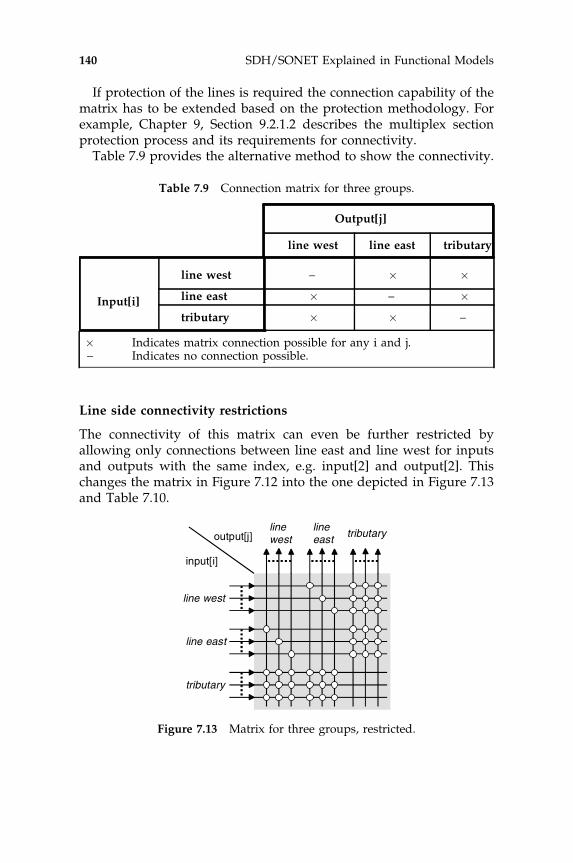
If protection of the lines is required the connection capability of thematrix has to be extended based on the protection methodology. Forexample, Chapter 9, Section 9.2.1.2 describes the multiplex sectionprotection process and its requirements for connectivity.

Table 7.9 provides the alternative method to show the connectivity.

Line side connectivity restrictions

The connectivity of this matrix can even be further restricted byallowing only connections between line east and line west for inputsand outputs with the same index, e.g. input[2] and output[2]. Thischanges the matrix in Figure 7.12 into the one depicted in Figure 7.13and Table 7.10.

Table 7.9 Connection matrix for three groups.

Output[j]

line west line east tributary

Input[i]

line west – � �line east � – �tributary � � –

� Indicates matrix connection possible for any i and j.– Indicates no connection possible.

input[i]

output[j]

line west

lineeast tributary

tributary

linewest

line east

Figure 7.13 Matrix for three groups, restricted.


Tributary side connectivity restrictions

Another form of restriction is also possible. Instead of restricting theconnectivity at the line side of the matrix, the add/drop capability isrestricted to a limited number of line inputs and outputs. In thisexample, the tributaries can be connected only to input[1] and out-put[1] of the east and west line. This changes the matrix in Figure 7.12into the one depicted in Figure 7.14 and Table 7.11.

Table 7.10 Connection matrix for three groups; line access restrictions.

Output[j]


Input[i]

line west – i¼ j �line east i¼ j – �tributary � � –


input[i]

output[j]

line west

lineeast tributary

tributary

linewest

line east

Figure 7.14 Matrix for three groups, trib. access restricted.


The functional model of a connection matrix for three groups isprovided in Figure 7.15. Note that the restrictions are not indicated inthis model.

Table 7.11 Connection matrix for three groups; trib. access restriction.

Output[j]


Input[i]

line west – � i¼ 1

line east � – i¼ 1

tributary j¼ 1 j¼ 1 –


<layer>_C

P[j] P[j]

P[i]

add/drop or tributary

line westP[i]

line east

Figure 7.15 Functional model of matrix for three groups.


8

Connection supervision


One of the criteria that was set right at the start of the development ofthe SDH and SONET multiplexing methodology was that the ‘Qualityof Service’ (QoS) should be improved. The PDH multiplexes providedhardly any possibility of checking the QoS for the transported signals.The addition of the ‘Cyclic Redundancy Checking’ (CRC) to the2.048 kbit/s signals defined in ITU-T Rec. G.706 (1991) were a steptowards providing QoS in PDH. To monitor the integrity of thetransported signals in SDH, SONET, OTN, etc., specific methodologiescan be applied. This chapter will describe some of the methods that canbe used to get information about the QoS or performance of a trail orconnection.

8.1 QUALITY OF SERVICE

Supervisory processes are required to assess the Quality of Service.These processes analyze the actual occurrence of a disturbance or faultof the transported signal with the purpose of providing an appropriateindication of the performance of the information transfer to the net-work operator. This type of performance should not be confused withthe performance regarding clock accuracy, jitter and wander, signalamplitude, and eye-patterns, that is, properties that are normallymonitored by external measuring equipment. Generally, the processof monitoring the error performance consists of the collection, analysis,


and reporting of performance information. Normally, each transportentity has its own associated monitoring process. All the performanceprocesses should run continuously to provide the most reliable and upto date information. The performance information will be retrievedfrom trail termination, adaptation and connection functions in theform of performance parameters. The parameters are accumulatedduring predetermined periods of time. Which functions are capable ofgathering, storing, thresholding and reporting these parameters istechnology dependent. The performance history can be correlatedand used to determine whether part of a network element has to bereplaced because it has degraded to a preset level. It can also beinterpreted and used to verify that Service Level Agreements (SLA)between network operators and clients are met. The latter applicationof performance monitoring is related mainly to network connections;this will be elaborated in the following sections.

8.2 CONNECTION MONITORING METHODS

In this section, four methodologies are described that can be used tomonitor the performance of a connection or a trail in a network, i.e. byinherent monitoring, non-intrusive monitoring, intrusive monitoringor sublayer monitoring.

Figure 8.1 shows only a specific fragment of a transport network, i.e.the part that is sufficient to illustrate the methodologies explained inthis chapter. It is the part that is located between a client trail and a

TCP

AP

TCP

APclient trail

LC

Network Connection

SNCSNC LCLC

server trailserver trailserver trail

CP CP

SNCSNC

Figure 8.1 Functional model fragment.


server trail. Figure 8.1 shows four network elements, two elements arethe nodes where the client trail starts and ends and two elements arepossible intermediate nodes. The intermediate nodes are included toillustrate the possibility that there is more than one server trail.

8.2.1 Inherent monitoring

This methodology monitors trails indirectly. In this case, the perfor-mance data that are available inherently from the server layer networkare used. Figure 8.1 can be used to illustrate this method because noadditional functionality is required.

If one of the associated server trails in one of the server layernetworks fails it may provide an indication of the failure (e.g. AIS)at the output of the link connection LC that is supported by the servertrail. This indication is forwarded, in sequence, over the next linkconnection that is supported by other trails in the server layer. Theoutput of the last link connection in the network connection mayprovide a trail signal fail indication.

Note that in SDH and OTN, the output of each Sn or ODUk linkconnection is able to detect the AIS to indicate that the transportthrough one of the preceding trails in the server layer has failed. Theoutputs of link connections in ATM and PDH are not able to detect thisfailure indication.

It is possible to collect error performance information for eachindividual link connection in the server layer network. When theserver layer adaptation function multiplexes more than one clientsignal, the error performance information for each of the link connec-tions, supported by the server layer trail, will not be availableindividually; it must be estimated from the error performance of theserver trail. Processes in the management network may correlate theperformance information collected from each link connection that ispart of the overall connection of interest. Since it does not include theperformance of the server layer adaptation and connection functionsthe overall error performance or QoS of the client trail cannot beprovided by this monitoring methodology.

8.2.2 Non-intrusive monitoring

This methodology monitors a client trail directly. In this case specialtermination functions monitor the characteristic information of the

Connection supervision 145

client trail. These special termination functions only have an input forthe signal to be monitored non-intrusively and are generally referredto as monitoring termination functions <signal>m_TT. They are con-nected to the client signal in the connection function as illustrated inFigures 8.2 and 8.3. The latter is a uni-directional representation of theconnection function depicting the actual matrix connections requiredto connect the non-intrusive monitors.

The performance information collected by the monitoring trailterminations can be retrieved to provide the QoS of the client trail.

AP APclient trail

LC SNC LCLC

server trailserver trailserver trail

CP CP

SNC

m m m m

Figure 8.2 Non-intrusive monitoring.

m

CP

m

TCP

Figure 8.3 Connection configuration.


The retrieved information concerns the connection from the originat-ing trail termination source function up to the point where the monitoris connected. It is also possible to monitor a specific part of a networkconnection by connecting monitors in connection functions of inter-mediate nodes. Processes in the management network may correlatethe performance data retrieved from these intermediate monitors toderive the performance of a specific section, e.g. a section that is part ofa different operator’s network. It is even possible to use this correlationmethodology to monitor arbitrary nesting or overlapping of networkconnection sections. Apart from the performance, the connectivity of asegment can also be checked by the monitors and used for faultlocalization. However, this requires proper identification of the mon-itored signal; in SDH the Trail Trace Identifier (TTI) is used for thispurpose.

8.2.3 Intrusive monitoring

This methodology monitors a normal, payload carrying client trail byinterrupting it to replace it by a test signal originating from a test trailtermination function <signal>t_TT function. This is depicted inFigures 8.4 and 8.5. The test trail can replace the client trail at anyarbitrary section of the network connection. Note that in order toswitch simultaneously this requires the synchronization of the con-nection functions at both source and sink side of the test trail.

AP AP(normal) client trail

LC SNCSNC

server trail

LCLC

server trailserver trail

CP CP

tt test trail

Figure 8.4 Intrusive monitoring.


Even though this method allows all parameters to be monitoreddirectly, the disadvantage is that the client trail is interrupted and thusaffects the availability of client signal, i.e. the QoS is degraded.Intrusive monitoring can only be performed during the setup phaseof a client trail, e.g. to test the performance or connectivity of the paththrough the network.

This method also supports arbitrary nesting or overlapping of thenetwork connections, but no simultaneous testing.

8.2.4 Sublayer monitoring

This methodology uses the functional modeling capability to create asublayer by expanding a connection point as described in Chapter 4,Section 4.2.3. Since a connection point is associated with a connectionfunction, the sublayer adaptation function <sublayer>/<client>s_Aand sublayer trail termination function <sublayer>s_TT can bedepicted either collapsed (as shown in Figure 8.6) or expanded (asshown in Figure 8.7). The <sublayer>s_TT function has the capabilityto monitor the sublayer trail. This capability depends on the usedtechnology, e.g. in SDH it uses a dedicated part of the trail OA&Moverhead and in packet networks it may use specific OA&M packets.The sublayer can be created in any two nodes in the network connec-tion to monitor the enclosed section. Intermediate nodes locatedbetween these two nodes shall transfer the specific OA&M transpar-ently.

This method allows all performance parameters to be tested directlyassuming that the used technology offers this OA&M capability. Thismethod also allows the nesting of monitored sublayer trails again

CP

TCP TCP

t

CP

TCP TCP

t

'normal' 'test'

Figure 8.5 Normal and test connection.


assuming that the technology supports this nesting, e.g. SDH allowsone level of nesting.

8.3 CONNECTION MONITORING APPLICATIONS

As already mentioned in the introduction of this chapter, performancemonitoring is used to check and guarantee the desired QoS, especiallyfor existing connections. However, to avoid connecting a client signal

AP APclient trail

LC SNCSNC SNCSNC

server trail

LCLC


CP CP

sublayer trail

Figure 8.6 Sublayer monitoring.

AP

CP

TCP

mon

itor

subl

ayer

sublayer trail

<sublayer>s_TT

<sublayer>/<client>s_A

Figure 8.7 Monitoring sublayer.


to a network connection that is already degrading, unused connectionscan be monitored for their quality. When a trail does not run com-pletely in a single operator’s network but passes another operator’snetwork, service level agreements (SLA) between the two are closed.Part of such an agreement will be the delivered QoS and this has to bemonitored from ingress to egress of part of the trail, i.e. the tandemconnection.

8.3.1 Monitoring of unused connections

A connection is unused if at least one of the access points that delimitsthe trail connection is not bound to a client signal adaptation function(see Figure 8.8).

A supervisory unequipped trail termination function <trail>s_TTcan be used to monitor unused connections. The source functiontransmits a layer characteristic information structure with an unde-fined payload and valid trail overhead; the sink function reports theperformance monitoring information to the element managementsystem. Remote information is exchanged between the sink and sourcefunction as shown in detail in Figure 8.9.

Note that any regular trail termination function may be used as asupervisory trail termination function if it can be operated without apayload signal.

AP

LC SNCSNC

server trail

LCLC


CP CP

ss unused trailor

Figure 8.8 Monitoring unused connection.


8.3.2 Tandem connection monitoring

A tandem connection monitoring provides the capability to monitor asection of a trail independent of the performance monitoring of thecomplete trail, as shown in Figure 8.10.

To be able to offer this capability, the tandem connection process hasto meet the following requirements:

� The tandem connection specific overhead (TC-OH) shall be insertedat the near-end and removed at the far-end of a tandem connection.

� The tandem connection process at the near-end shall report theperformance and failure/alarm conditions related to the incomingsignal for the purpose of fault localization; this information is alsoforwarded to the far-end in the TC-OH.

� The tandem connection process at the far-end shall report theperformance and failure/alarm conditions related to the incomingsignal for the purpose of fault localization, e.g. by correlating thebit-error rate detected at near-end and far-end, the bit-error rate ofthe tandem connection can be derived.

s

CP

sRDIREI

TCP

Figure 8.9 Supervisory unequipped.

TC_OH

client trail

nearend

tandem connection

farend

TC_OH

Figure 8.10 Tandem connection monitoring.


� The tandem connection monitoring shall be independent of anyincoming server signal fail indication, e.g. AIS, FDI.

� The tandem connection process at the near-end shall report andforward a detected incoming server signal fail indication for thepurpose of fault localization, e.g. before or after the near-end.

� The tandem connection process at the far-end shall report andforward a detected incoming server signal fail indication for thepurpose of fault localization, e.g. before or after the far-end.

� The tandem connection connectivity between near-end and far-endshall be traceable, i.e. each tandem connection shall have its ownspecific Access Point Identifier (API).

� The tandem connection process shall report continuity defects, i.e.loss of signal, unequipped signal, and API mismatch, detectedbetween the near-end and the far-end.

Several applications of tandem connections are possible; threepossible applications are described below:

� A tandem connection can monitor the quality of the servicedelivered to a client. This is an application in a public networkdomain, a network operator domain, a network operator sub-network domain, etc. Generally it is referred to as a serving operatoradministrative domain. The functional model is depicted in Figure 8.11.In this application the supporting tandem connection has itssublayer source functions as close as possible behind the user tonetwork interface (UNI) or network to network interface (NNI), and itssublayer sink functions as close as possible in front of the UNI orNNI.

tandem connection

client trail

LCSNC SNCSNCSNCSNC SNC

sublayer trail

UNI or NNIUNI or NNI

LCLC LCLC

Figure 8.11 Serving operator administrative domain.


� Two tandem connections can be used to monitor the defect status ofthe working and protection network connections. Normally, thisapplication is called a protected domain; the sublayer monitored SNCprotection methodology is described in Chapter 9, Section 9.2.2.1.The functional model of this application is shown in Figure 8.12. Aprotected domain utilizing tandem connections has its sublayersources right behind the protection switch bridge and its sublayersinks just in front of the protection switch selector functions.

� A tandem connection can monitor the quality of the service of asection of a client trail. In a user domain this can be the service

tandem connection

client trail

LCSNC

SNCSNCSNC

SNC

sublayer trail

LC LCLC

tandem connection

LCSNC SNC

LCLC

sublayer trail

Figure 8.12 Protective domain.

tandem connection

client trail

LCSNC SNCSNCSNCSNC SNC

sublayer trail

UNI or NNIUNI or NNI

LC LC LCLC

Figure 8.13 Service requesting administrative domain.


provided by the operator; in an operator domain this can be theservice provided by a second operator. In general, it is referred to asa service requesting administrative domain. The functional model isprovided in Figure 8.13. The tandem connection in this applicationhas its sublayer source function as close as possible in front of theUNI or NNI, and its sublayer sink function as close as possiblebehind the UNI or NNI.


9

Protection models

This chapter describes the functional models that can be used to modelthe protection schemes in a layered network. Generally, these protectionschemes are used to improve the availability of a client signal. Theavailability is one of the components of a service agreement betweenoperators or a performance requirement for network equipment.

9.1. INTRODUCTION

The modeling methodology used to describe a transport network canbe utilized to illustrate one of the main strategies that are used toimprove the availability of such a network. Availability is the ability ofa transport network to be in such a state that it can transfer informa-tion under required performance conditions during a given timeinterval, assuming that the required resources are provided or, at itssimplest level:

Availability ¼ Uptime=ðUptimeþDowntimeÞ

The availability of a telecommunications network or a trail in atransport network is ideally 100%, however, due to physical propertiesand human errors the availability is usually lower if no specialmeasures are taken. From a design or implementation point of viewthe availability can be expressed as:

Availability ¼MTBF=ðMTBFþMTTRÞ


where MTBF is the Mean Time Between Failures of the used transportentities and MTTR is the Mean Time To Repair those resources. Theavailability can be improved by providing a replacement for the failedor degraded transport entities, such as equipment or interconnectingfibers. Now, the availability is determined mainly by the time it takesto replace the failed or degraded resources, i.e. the MTTR. Decreasingthe MTTR will increase the availability of the network. The use of thesereplacing transport entities is normally a consequent action based ondetection of a defect or of a degraded performance. The replacementcan also be based on an external request, e.g. a command issued by anoperator at a network management system.

Two types of replacement can be distinguished:

� Replacement by protection.This type of replacement utilizes pre-allocated capacity betweentwo or more nodes in the network that is dedicated to protection.Normally, a stand-by or protection transport entity will replace theoriginal, or working transport entity. The architecture dedicated tothis type of replacement can have different grades of complexity. Inits most simple form the architecture has a single dedicatedprotection entity to replace each working entity (1þ 1) and isnormally referred to as one-to-one protection (see Figure 9.1).

Normally, this form of protection is single ended because theselection between working or protection entity is performed at thereceiving end only. At the sending end the information is distrib-uted or bridged over both working and protection entities.

When the protection entity is not in use because the workingentity is carrying the client information or normal traffic, its

working entity

protection entity

normal traffic

protection entity

normal traffic

normal condition

protection condition

failed

Figure 9.1 1þ 1 protection.


capacity can be used to transport extra traffic. This type of protec-tion is referred to as (1:1) or one-by-one protection and is illustrated inFigure 9.2.

Now, the sending end has to know which transport entity thereceiving end has selected. For this purpose an Automatic ProtectionSwitch (APS) channel has been defined and an APS protocol wasdeveloped to align the receiving and sending end of the transportentity.

When the failed working entity has been repaired this will bedetected at the receiving end and normally the protection switchreturns to its original position: the protection switch is revertive asillustrated in Figure 9.2. However, this will most probably cause ahit, i.e. bit-errors, in the transported information.

In case this is not acceptable, it is possible to implement orprovision the protection switch to be non-revertive: after eachprotection switch the designation of working and protection tothe interconnecting entities will be switched as well. Figure 9.3shows the non-revertive protection switch.

working entity

protection entity

normal traffic

extra traffic

protection entity

normal traffic

extra traffic

normal condition

protection condition

failed

APS channel

APS channel

working entity

protection entity

normal traffic

extra traffic

reverted to normal condition

APS channel

Figure 9.2 1:1 protection; revertive.

Protection models 157

In its most complicated form the architecture has m separateprotection entities to replace n working entities (m:n), normallyreferred to as n by m protection (see Figure 9.4).

Replacement or protection switching can be either uni-directionalor bi-directional. Uni-directional protection switching replaces theaffected transport entities only in the affected transport direction inthe case of a uni-directional failure. Bi-directional protectionswitching replaces not only the affected transport entity in thefailed directions but also replaces the (unaffected) transport entityin the opposite direction.

� Replacement by restoration.This type of replacement utilizes any spare capacity availablebetween nodes in the network. In general, restoration requiresalgorithms that utilize re-routing of transport entities. Whenrestoration is used in a transport network a certain percentage ofthe network capacity has to be reserved for the re-routing of theworking traffic. Since this type of replacement cannot be describedusing the functional model it will not be discussed in more detail inthis book.

working entity

protecting entity

normal traffic

extra traffic

working entity

normal traffic

extra traffic

initial condition

switched condition

failed

APS channel

APS channel

working entity

normal traffic

extra traffic

new condition

APS channel

protecting entity

Figure 9.3 1:1 protection; non-revertive.


9.2. PROTECTION

When SDH technology was introduced new network topologies werealso introduced in the transport domain, one of the most remarkablebeing the ring. An SDH ring is comprised of a number of networkelements that allow traffic to ingress, to egress the ring or pass throughthe ring. This equipment is commonly referred to as Add/Drop Multi-plexers (ADM). The ADMs are interconnected in a loop configurationas illustrated in Figure 9.5.

This network topology is particularly suitable for providing protec-tion to improve the availability of network resources.

1

.

.

.

.

.

.m

1..

..n

1...

.n

n APS channels

Figure 9.4 m:n protection.

ADMADM

ADM

ADMADM

traffic traffic

Figure 9.5 Typical SDH ring architecture.


Within the transport network architecture two distinctive types ofprotection can be identified: trail protection and sub-network protection.

Protection architectures and mechanisms are defined and describedin separate recommendations, for SDH in ITU-T Rec. G.808.1 (2003)and for OTN in ITU-T Rec. G.873.1 (2003). ITU-T Rec.G.842 (1997)describes the interworking of SDH protection architectures.

9.2.1 Trail protection

Trail protection is a protection method applied in a transport layernetwork when a defect condition is detected in the same layer network(i.e. protection switching is activated in the same transport layernetwork).

A signal selected to be protected, i.e. the protected trail, consists of the(original) working trail that will be replaced by the protecting trail if theworking trail fails or if its performance falls below the required level.The required level is usually described in an SLA (service levelagreement) between a server (operator) and a client (customer). Twotypes of trail protection will be described:

1. path level, protecting a network connection; and2. multiplex section or line level, protecting the sections in a ring of

nodes in a network.

9.2.1.1 Path level trail protection

This type of trail protection is modeled by introducing a protectionsublayer. The original trail termination (TT), as shown in the shadedarea in Figure 9.6, is expanded according to the rules given inChapter 4, Section 4.2.2.

The result is shown in Figures 9.7a and 9.7b for 1þ 1 protection andFigures 9.8a and 9.8b for 1:1 protection. The protection adaptationfunctions Ap, the unprotected trail termination functions TTu, theprotected trail termination functions TTp and a protection connectionfunction Cp are introduced to model the switching between theprotecting and working connections. The introduced adaptation, trailtermination and connection functions are bound by the additionalprotection access points APp, the protection termination connectionpoints TCPp and the connection points CP. The status of the trails inthe protection sublayer is made available to the protection connection


function Cp, i.e. the Trail Signal Fail/Degrade (SF/SD) signal in Figures9.7a, 9.7b, 9.8a and 9.8b by the unprotected trail termination TTu. If theprotection mechanism requires communication between the controlfunctions of the protection connection functions, the protection adap-tation function may provide access to an Automatic Protection Switch(APS) channel. The protected trail termination TTp provides the statusof the protected trail.

Figures 9.7a and 9.7b show the model for 1þ 1 trail protection. Theshaded area indicates the protection sublayer that replaces the trailtermination functions shown in the shaded area in Figure 9.6. Asmentioned before, this type of protection is normally single-ended oruni-directional. The receiving end determines whether the working orprotecting (sub-)network connection is used and if the use of the APSchannel is not required. If both forward and return trail switching isrequired simultaneously at the near-end and far-end, i.e. bi-directionalprotection switching, the APS channel has to be used. In this case theprotection switching protocol can be optimized depending on thepredominant protection switching methodology (1þ 1 or 1:1) (formore details, see ITU-T Rec. G.841 (1998)).

Figures 9.8a and 9.8b show the model for 1:1 trail protection. Theshaded area indicates the protection sublayer that replaces the trailtermination functions shown in the shaded area in Figure 9.6 for boththe normal traffic trail and for the extra traffic trail.

Normally, this type of protection is bi-directional and uses the APSchannel for synchronizing the near-end and far-end of the trails. In thecase of uni-directional use, the protection switch is based on localconditions and requests only; the near-end and far-end operate

sub-network connection

trail

TT TT

TCP

TCP

AP AP

AA

TT TT

TCP

TCP

AP AP

AA

Figure 9.6 Unprotected trail.


(working)

protecting

working trail

RDI

REI

RDI

REI

protecting trail

protected trail

SF/SD SF/SD

APSAPS

protectionlayernetwork

TTpTTp

TTu TTu

TTuTTu

ApAp

Cp

TCP

TCP

TCP

TCP

TCPp TCPp

APp APp

APpAPp

AP AP

CP CPCPCP

AA

Ap Ap

Figure 9.7a 1þ 1 trail protection (near-end).


network connection

RDI

REI

RDI

REI

SF/SDSF/SD

APSAPS

network connection

protectionlayer

network

AP

TTp

TCPp

CP

APp

TTu

TCP

Ap

A A

AP

TTp

TTu

APpAPp

APp

TCP

ApApAp

TCPp

Cp

CPCPCP

Figure 9.7b 1þ 1 trail protection (far-end).


(working)

protecting

working trail

RDI

REI

RDI

REI

protecting trail

protected trail

SF/SD SF/SD

APSAPS

extra trafficnormal traffic

Figure 9.8a 1:1 trail protection (near-end).


network connection

network connection

RDI

REI

RDI

REI

SF/SDSF/SD

APSAPS

extra trafficnormal traffic

Figure 9.8b 1:1 trail protection (far-end).


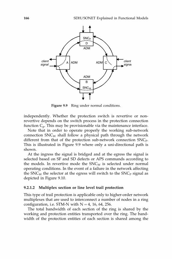
independently. Whether the protection switch is revertive or non-revertive depends on the switch process in the protection connectionfunction Cp. This may be provisionable via the maintenance interface.

Note that in order to operate properly the working sub-networkconnection SNCW shall follow a physical path through the networkdifferent from that of the protection sub-network connection SNCP.This is illustrated in Figure 9.9 where only a uni-directional path isshown.

At the ingress the signal is bridged and at the egress the signal isselected based on SF and SD defects or APS commands according tothe models. In revertive mode the SNCW is selected under normaloperating conditions. In the event of a failure in the network affectingthe SNCW the selector at the egress will switch to the SNCP signal asdepicted in Figure 9.10.

9.2.1.2 Multiplex section or line level trail protection

This type of trail protection is applicable only to higher-order networkmultiplexes that are used to interconnect a number of nodes in a ringconfiguration, i.e. STM-N with N¼ 4, 16, 64, 256.

The total bandwidth of each section of the ring is shared by theworking and protection entities transported over the ring. The band-width of the protection entities of each section is shared among the

A

ADM

C

B

D

ADMADM

ADM

clientsignal

SNCP

SNCW

clientsignal

Figure 9.9 Ring under normal conditions.


working entities of all sections of the ring. The client signals aretransported bi-directionally over the ring and follow the same physicalpath; together with sharing the protection bandwidth this gives abetter utilization of the total bandwidth in the ring. Figure 9.11 shows

A

ADM

C

B

D

ADMADM

ADM

clientsignal

SNCP

SNCW

clientsignal

Figure 9.10 Failure in a ring section.

A

ADM

clientsignal

C

B

D

ADMADM

ADM

clientsignal

Figure 9.11 Client singal path in MS protection.


an example of this type of protection in an SDH ring transporting aclient signal.

This type of trail protection is also modeled by introducing aprotection sublayer. The original section to path adaptation, MSn/Sn_A as shown in the shaded area in Figure 9.12, is expandedaccording to the rules given in Chapter 4, Section 4.2.1. The result isshown in Figure 9.13.

Note: Figure 9.12 shows a simplified model of node i in a networktopology consisting of a ring of nodes; each node is connected to twoother nodes. The value of N¼ 4, 16, 64, 256. The value of x is arbitrary.In the connection function, Sn_C signals are either added to, droppedfrom or passed through the two multiplex section adaptation functionsMSn/Sn_A.

The protection adaptation functions MSp/Sn_A, the protectiontrail termination functions MSp_TT, the protected trail terminationfunctions MS/MSp_A and an MS protection connection function MSpare introduced to model the MS – shared protection ring (MS-SPRing)switching. This type of trail protection requires a communicationprotocol between the control functions of the protection connectionfunctions; the protection adaptation function MS/MSp_A shall pro-vide access to an Automatic Protection Switch (APS) channel.

With this type of trail protection a distinction is made for the type oftraffic that will be transported over the multiplex section betweenadjacent nodes:

to

node (i −1)

normal traffic

to

node (i+1)MSn_TT MSn_TT

MSn/Sn_A

1 . . . . . . . . . . . . . . . . . . . . . . . . . . . . . . . . . . . . . . . x

1 . . . . N . . . .MSn/Sn_A

Sn_TT Sn_TT

Sn_C

node i

N1

Figure 9.12 Unprotected consideration.


� normal traffic; this is the traffic than will be protected and will havethe highest availability figure. It is transported in the workingchannel (‘w’ in Figure 9.13).

� extra traffic; this is the traffic that will be discarded as soon asprotection of the normal traffic is required. It will have the lowestavailability of the three channels because every protection switch inthe ring affects it. The extra traffic is transported in the protectionchannel (‘p’ in Figure 9.13).

� non-pre-emptible unprotected traffic (NUT); this is the traffic thatwill not be affected by the trail protection switching. It will have anavailability figure between that of the working channel and theprotection channel as it will be affected only by a defect in a multiplexsection. The NUT traffic may have its own (trail) protection

to

node (i −1)

APSAPS

normal trafficextra traffic

to

node (i+1)MS_TTM S_TT

MS/MSp_A

NUTNUT

MS/MSp_A

MSp

MSp_TT

MSp/Sn_A

Sn_TT

node i

w p n n p w

Sn

ab

aa

baa

Figure 9.13 MS-shared protection ring.


mechanism; excluding it will prevent nesting of protectionschemes. The NUT channel (‘n’ in Figure 9.13) carries the NUT.

The maximum payload capacity of the working channel is equal tothe capacity of the protection channel, as indicated by ‘a’ in the Snconnection function in Figure 9.13. The payload capacity of the NUTchannel is different from the working and protection channel and isindicated by ‘b’ in Figure 9.13. The values ‘a’ and ‘b’ represent themaximum number of signals Sn that may be transported by a channel.The values ‘a’ and ‘b’ are provisioned to have the same value in allnodes of the ring. Note that all ‘a’ and ‘b’ signals Sn drawn in the Snconnection function either originate locally or are passed through fromnode (i� 1) to node (iþ 1) and vice versa. In the Sn connection,function switch capacity has to be reserved to pass through theprotection channel in case of a protection switch in the ring. It shallhave the same capacity as the protection channel: ‘a’ Sn signals.

For an STM-N (N¼ 4, 16, 64, 256) the following limits apply:1� a�N/2, 0� b<N and (2aþ b)<N.

Figure 9.14 shows the configuration of node i, especially the MSpconnection function, after a fault has occurred on the ring sectionbetween node i and node (iþ 1) and the protection switch has beenperformed. The working traffic towards node (iþ 1) will replace theextra traffic on the protection channel towards node (i� 1); the switchtime determines the MTTR of the working channel. The objective isthat it is less than 50ms, see ITU-T Rec. G.841 (1998) clause 7.2.2. Allthe extra traffic in node i will be interrupted and the NUT to and fromnode (iþ 1) will be interrupted affecting their availability; the MTTR isdetermined by the time it takes to repair physically the faulty section.The equivalent (mirrored) configuration will be found in node (iþ 1).

Figure 9.15 shows the configuration of node i, especially the MSpconnection function, after a fault has occurred on a ring section notconnected to node i. To be more precise: if in an STM-N ring one of thesections experiences a fault condition that requires an MS-SPRingprotection switch, the two nodes connected to the faulty section willhave the switch configuration depicted in Figure 9.14 and all othernodes in the ring will have the configuration depicted in Figure 9.15. Inthis configuration the protection traffic received from node (iþ 1) willbe passed through to node (i� 1) and vice versa using the reservedpass-through capacity of the Sn connection function. All the extratraffic in node i will be interrupted. (Note: the NUT is not affected inthis node.)


9.2.2 Sub-network connection protection

Sub-Network Connection Protection (SNCP) is a protection mechanismthat may be used in any network topology, e.g. mesh, ring or mixedmesh/ring. It is applicable in any path layer in a layered network. Itmay be used to protect a path between two Termination ConnectionPoints (TCP). However, this is useful only when there are two diverseroutes available through the network. Figure 9.16 shows a typical SDHnetwork topology: a ring comprised of network elements intercon-nected by fibers transporting STM-N signals.

At the originating TCP in node i the characteristic information isbridged and sent in both directions on the ring, one signal via node(i� 1) and the other via node (iþ 1). At the receiving TCP in node z a

to

node (i −1)

APSAPS


to

node (i+1)MS_TTM S_TT

MS/MSp_A

NUTNUT

MS/MSp_A

MSp

MSp_TT

MSp/Sn_A

Sn_TT

node i

w p n n p w

Sn

ab a

ab aa

Figure 9.14 MS-SPRing adjacent node protecting.


selector is used to select one of these signals based on the performanceof either path, e.g. SF or SD.

This protection methodology is also applicable to a part of a pathbetween two Connections Points (CP) or between a CP and a TCPprovided again that two diverse routes are available. It is even possiblethat the sub-network connection being protected is made up of asequence of protected sub-network connections and link connections.

SNCP switching is a methodology that is applied in the client layernetwork whenever a defect condition is detected in a server layernetwork, a server sublayer network or another server transport layernetwork. In other words it is based on server layer performance.Currently, SNCP switching is defined to be uni-directional only; bi-directional SNCP is for further study as well as the use of the

to

node (i −1)

APSAPS


to

node (i+1)MS_TT MS_TT

MS/MSp_A

NUTNUT

MS/MSp_A

MSp

MSp_TT

MSp/Sn_A

Sn_TT

node i

w p n n p w

Sn

ab a

ab aa

Figure 9.15 MS-SPRing non-adjacent node protecting.


protection bandwidth for transporting extra traffic during normaloperation. This means that no APS channel is required.

SNCP schemes can be characterized by the monitoring method usedto derive the switching criteria:

� sub-layer monitoring by expanding the sub-network connectionpoints;

� inherent monitoring by using server layer performance informa-tion;

� non-intrusive monitoring by adding client layer monitoring func-tions.

The signal that is provisioned to be protected, in this case referred toas a working (sub-)network connection, is replaced by a protecting(sub-)network connection if the working (sub-)network connectionfails or if its performance falls below the required level.

9.2.2.1 Sublayer trail monitoring:

This SNCP scheme, sometimes referred to as SNC/S, can be modeledby expanding the sub-network connection points and inserting a

i

ADM

z

i+1

i−1

ADMADM

ADM

clientsignal

SNCP

SNCW

clientsignal

Figure 9.16 Ring with diverse routed client signal.


protection sublayer, according to the rules given in Chapter 4, Section4.2.3. The introduction of a sublayer results in a trail protection of thesublayer trail that runs between the protection access points APp. Thisis illustrated in Figures 9.17a and 9.17b; the inserted protectionsublayer is shown in the shaded area. The original connection pointis split into a protection connection point CPp and a protectiontermination connection point TCPp. In this inserted sublayer theprotection trail termination function TTp provides the monitoring ofthe performance of the server signal. (See also Chapter 8, Section 8.2.4.)The monitoring results in a server signal fail (SF) or server signaldegraded (SD) signal that is forwarded by the protection adaptation

(working)

protectingRDI

REI

RDI

REI

protected (sub)

SFSD SF/SDCP

TCP

CPp

CPp

APp

Ap

TTpprot

ectio

n su

blay

er

Sn

serv

er la

yer

netw

ork

clie

nt la

yer

netw

ork

sublayer

trail

sublayer

trail

Figure 9.17a SNC protection by sub-layering.


function Ap to the client layer connection function Sn. This Sn willexecute the protection switch.

9.2.2.2 Inherent monitoring

This SNCP scheme, normally referred to as SNC/I, can be modeled byshowing the server layer performance information derived by theserver layer network as described in Chapter 8, Section 8.2.1. Theserver layer signal condition is used to initiate the protection switch inthe client layer. This is illustrated in Figures 9.18a and 9.18b by theshaded area.

RDI

REI

RDI

REI

SF/SD SF/SD

clientlayer network

Sn

CP

TCP

CPp

CPp

APp

Ap

TTp

sublayer

trail sublayer

trail

network connection


SNC

protection sublayer

Figure 9.17b SNC protection by sub-layering (continued).


(working)

protectingRDI

REI

RDI

REI

protected (sub)

SF/SD SF/SD

Sn

TT

A

TT

A

serv

er la

yer

netw

ork

clie

nt la

yer

netw

ork

Figure 9.18a SNC protecion by inherent monitoring: SNC/I (continued).

(working)

protectingRDI

REI

RDI

REI

protected (sub)

SF/SD SF/SD

TTmTTm

TT

TT

A A

serv

er la

yer

netw

ork

clie

nt la

yer

netw

ork

Sn

Figure 9.19a SNC protection by non-intrusive monitoring: SNC/N.


RDI

REI

RDI

REI

SF/SD SF/SD

Sn

TT

A

TT

A

network connection

SNC


Figure 9.18b SNC protecion by inherent monitoring: SNC/I.

RDI

REI

RDI

REI

SF/SD SF/SD

TT

A A

TT

TTm TTm

Sn

network connection

SNC


Figure 9.19b SNC protection by non-intrusive monitoring: SNC/N (continued).


The monitoring capabilities of the existing trail termination (TT) isused in the SNC/I scheme. The TT monitors the performance of theserver layer (sub-)network connection and detects a server signal fail(SF) or server signal degraded (SD). The SF/SD signal is forwarded bythe server layer adaptation function A to the client layer connectionfunction Sn.

9.2.2.3 Non-intrusive monitoring

This SNCP scheme is generally referred to as SNC/N. In this case theserver layer network trail termination function (TT) has no capabilityto monitor the performance of the server layer. For the monitoring ofthe (sub-)network connection, listen-only trail termination functionsTTm are used. They are available in the client layer (or have to beadded as described in Chapter 8, Section 8.2.2) (see the shaded area inFigures 9.19a and 9.19b. These TTm are connected permanently to theserver signal received from the server adaptation function A (see thegray line in the same figures). A detected server signal failure (SF) orserver signal degraded (SD) will be reported to the client layerconnection function Sn to initiate a protection switch.

9.2.2.4 Intrusive monitoring

This SNCP methodology is not recommended for use as part of aprotection scheme. It is the same scheme as used in SNC/N except forthe permanent connection of the received server signal. In case ofintrusive monitoring, the received server signal is either passedthrough to the client layer termination function or it is (occasionally)switched to the monitoring function TTm to get the informationrequired to perform a protection switch. The client signal is inter-rupted during the monitoring phase. Depending on the frequency ofswitching for monitoring, this may severely affect the availability ofthe transported information. See also Chapter 8, Section 8.2.3 for adescription of intrusive monitoring.


10

Compound functional modelsand their decomposition

This chapter describes the compound functional models, and theirdecompositions. These compound functions were introduced at thetime Virtual Concatenation (VCAT) was defined in G.783 (2004).The compound function can be used in the general functional modelsthat describe transport equipment or networks; the implementers of thecompound functions can use the decomposed models. Three compoundfunctional models will be described in this chapter: the VCAT com-pound functions with Link Capacity Adjustment Scheme (LCAS)disabled; the VCAT compound function with LCAS enabled; and theVCAT to Contiguous Concatenation (CCAT) interworking compoundfunction. The VCAT compound function is a specific application of theinverse multiplexing described in Chapter 2, Section 2.5.2.

10.1 LCAS DISABLED VCAT FUNCTIONS

The virtual concatenated trail termination compound function thatdoes not support LCAS or has LCAS disabled is generally referred toas Sn–Xv_TT. It is represented by a compound functional model,which means that it is composed of a number of ‘standard’ atomicfunctions. The preferred symbol is depicted in Figure 10.1.

This model can be decomposed into the following atomic functions:the Sn–X Trail Termination function Sn–X_TT, the Sn–Xv to Sn–X


Adaptation function Sn–Xv/Sn–X_A and the X separate memberSn Trail Termination functions Sn_TT. Figure 10.2 illustrates thedecomposition.

This figure shows the bi-directional representation of the atomic func-tions. The transport of a signal is normally described uni-directionally

Sn-Xv_TT

Sn-Xv_CI

Sn-X_AI

1 . . . . . . . X

AP

CP

Figure 10.1 Sn–Xv_TT function.

Sn-Xv_TTSn-Xv/Sn-X_A

Sn-X_TT

Sn_TT Sn_TT

Sn-Xv_AI. . . . . . . . . = . . . . . . . . .

Sn_AI[1...X]

Sn_CI[1] Sn_CI[X]Sn-Xv_CI = Sn_CI[1...X]

Sn-X_AI

1 . . . . . . X

Sn-X_AI

1 . . . . . . . . . X

Sn-X_CI

AP

CP

CP

AP

CP

AP

CP CP

AP

Figure 10.2 Decomposition of the Sn-Xv_TT function.


as follows. A certain trail signal, i.e. the adapted informationSn–X_AI, will be transported through the network using virtualconcatenation. For this purpose it is connected at the source side tothe source side Sn–X_TT_So function. The source side Sn–Xv/Sn–X_A_So function takes care that the characteristic informationSn–X_CI, a contiguous signal, received from the Sn–X_TT functionwill be adapted for distribution over X trails. The adapted informa-tion Sn–Xv_AI is equivalent to the sum of the adapted informationSn_AI of the X individual trails. Each source side Sn_TT_So functionwill output the characteristic information Sn_CI that can be trans-ported individually through the network. In the opposite direction, theSn_CI signal received by the X individual sink side Sn_TT_Sk func-tions will be processed and sent to the sink side Sn–Xv/Sn–X_A_Skfunction to compose the concatenated characteristic informationSn–X_CI that will be processed by the sink side Sn–X_TT_Sk functionand output as the trail signal Sn–X_AI.

The following sections will describe the individual atomic functions.

10.1.1 Sn–Xv trail termination function

This is the generic virtual concatenation trail termination function thatdoes not support LCAS (or has LCAS disabled). It serves as thebeginning and end point of a contiguous trail signal that will betransported over X individual (sub-)network connections. Figure 10.3shows the bi-directional model.

Sn-Xv_TT

Sn-Xv_CI = Sn_CI[1... X]

Sn-X_AI

1 . . . . . . . X

Sn-X_AP

Sn_CP

Figure 10.3 Bi-directional Sn-Xv_TT function.

Compound functional models 181

Bi-directional model Sn–Xv_TT

The Adapted Information Sn–X_AI present at the Access point Sn–X_APis adapted for the transport over the network and distributed over theX individual Characteristic Information Sn_CI, passing the ConnectionPoints Sn_CP. The operation of the function is described in the nextsections of this chapter.

This model can be decomposed in the uni-directional models shownin Figures 10.4 and 10.5.

Source side: Sn–X_TT_So

Symbol

Interfaces

Processes

See the description of the individual atomic functions in the followingsections.

Sn-Xv_TT_So

Sn-Xv_CI = S n_CI[1...X]

Sn-X_AI

1 . . . . . . . X

Sn-X_So_AP

Sn_So_CP

Figure 10.4 Source side Sn-Xv_TT function.

Sn–Xv_TT_So.

inputs outputs

at Sn–X_So_AP at Sn_So_CPSn–X_AI_D Sn_CI[1. . .X]_DSn–X_AI_CK Sn_CI[1. . .X]_CKSn–X_AI_FS Sn_CI[1. . .X]_FS


Sink side: Sn–X_TT_Sk

Symbol

Interfaces

Processes

See the description of the individual atomic functions in the followingsections.

10.1.2 Sn–Xv/Sn–X adaptation function

This is the function that performs the adaptation of the con-tiguous client signal to the virtual concatenated server layersignals transported by the individual members of the Virtual Con-catenation Group (VCG). Figure 10.6 shows the bi-directional func-tional model.

Sn-Xv_TT_Sk

Sn-Xv_CI = Sn_CI[1...X]

Sn-X_AI

1 . . . . .. . X

Sn-X_Sk_AP

Sn_Sk_CP

Figure 10.5 Sink side Sn-Xv_TT function.

Sn–Xv_TT_Sk.

inputs outputs

at Sn–X_Sk_CP at Sn_Sk_APSn–X_CI_D Sn_AI[1. . .X]_DSn–X_CI_CK Sn_AI[1. . .X]_CKSn–X_CI_FS Sn_AI[1. . .X]_FS


Bi-directional model: Sn–Xv/Sn–X_A

Symbol

This model can be further decomposed into the uni-directional modelsdepicted in Figures 10.7 and 10.9.

Source side: Sn–Xv/Sn–X_A_So

The source side VCAT adaptation function performs the distributionof the incoming contiguous concatenated signal Sn–Xc received at theConnection Point as data signal Sn–X_CI_D (together with the asso-ciated clock Sn–X_CI_CK and frame start signal Sn–X_CI_FS) to con-stitute the virtual concatenated signal Sn–Xv transmitted at the AccessPoint as data signal Sn–Xv_AI_D. This signal is the equivalent of thecombined payload of the X individual member signals Sn transmittedas Sn_AI_D over themember Access Points, where X can have any value1� X� (max) (where (max) is technology specific, e.g. 256 for a VC–4).

Symbol

Sn-Xv/Sn-X_A

1 . . . . . . . X

Sn-Xv/Sn-X_A_MP

Sn-Xv_AI = Sn_AI[1...X]

Sn-X_CI

Sn-X_CP

Sn_AP

Figure 10.6 Bi-directional Sn-Xv/Sn-X_A function.

Sn-Xv/Sn-X_A_So


1 . . . . . . . X

Sn-X_CI

Sn-X_So_CP

Sn_So_AP

Figure 10.7 Source side Sn-Xv/Sn-X_A function.


Interfaces

Processes

This function performs the following processing between its input andoutput:

� distributes the received client signal round-robin octet-wise overthe payload area of all the members in the VCG;

� inserts the VCAT overhead information in each of the VCGmember signals, i.e. the multi-frame indication, sequence numberand CRC;

� inserts the payload type identification into the signal label of eachof the member signals.

The processes described above and their relations are depicted inFigure 10.8.

Sn–Xv/Sn–X_A_So.

inputs outputs

at Sn–X_So_CP at Sn_So_APSn–X_CI_D Sn_AI[1. . .X]_DSn–X_CI_CK Sn_AI[1. . .X]_CKSn–X_CI_FS Sn_AI[1. . .X]_FS

Sn-Xv_AP

Sn-X_CP

AI_

D

C2

distribution: octet by octet

CI_

D

payl

oad

PO

H

payl

oad

PO

H VC

AT

-OH

AI_

D

AI_

D

payl

oad

PO

H

1 2 .......... ...........X

Figure 10.8 Sn-Xv/Sn-X_A So processes.


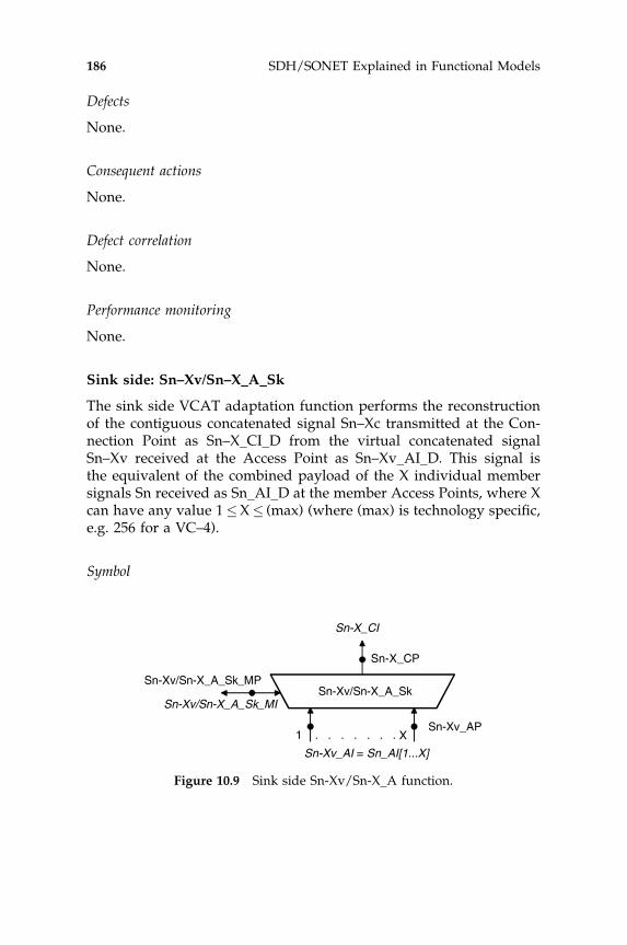
Defects

None.

Consequent actions

None.

Defect correlation

None.


None.

Sink side: Sn–Xv/Sn–X_A_Sk

The sink side VCAT adaptation function performs the reconstructionof the contiguous concatenated signal Sn–Xc transmitted at the Con-nection Point as Sn–X_CI_D from the virtual concatenated signalSn–Xv received at the Access Point as Sn–Xv_AI_D. This signal isthe equivalent of the combined payload of the X individual membersignals Sn received as Sn_AI_D at the member Access Points, where Xcan have any value 1�X� (max) (where (max) is technology specific,e.g. 256 for a VC–4).

Symbol

Sn-Xv/Sn-X_A_Sk


1 . . . . . . . X

Sn-X_CI

Sn-Xv/Sn-X_A_Sk_MI

Sn-X_CP

Sn-Xv_AP

Sn-Xv/Sn-X_A_Sk_MP

Figure 10.9 Sink side Sn-Xv/Sn-X_A function.


Interfaces

Processes

This function performs the following processing between its input andoutput:

� verifies the payload type identification in the signal label of each ofthe member signals;

� buffers the received signal of each individual VCG mem-ber to compensate the differential delay due to diverserouting;

� assembles the original client payload signal from the memberoctets after using the multi-frame indication for re-alignment andthe sequence number for re-sequencing the individual membersignals;

� forwards a received Trail Signal Fail (TSF) indication to the nextfunction as Server Signal Fail (SSF).


Sn–Xv/Sn–X_A_Sk

inputs outputs

at Sn_Sk_AP at Sn_Sk_CP

Sn_AI[1. . .X]_D Sn–X_CI_DSn_AI[1. . .X]_CK Sn–X_CI_CKSn_AI[1. . .X]_FS Sn–X_CI_FSSn_AI[1. . .X]_TSF Sn–X_CI_SSF

at Sn–Xv/Sn–X_A_Sk_MP

Sn–Xv/Sn–X_A_Sk_MI_cPLM[1. . .X]Sn–Xv/Sn–X_A_Sk_MI_AcSL[1. . .X]Sn–Xv/Sn–X_A_Sk_MI_AcSQ[1. . .X]Sn–Xv/Sn–X_A_Sk_MI_cLOM[1. . .X]Sn–Xv/Sn–X_A_Sk_MI_cSQM[1. . .X]Sn–Xv/Sn–X_A_Sk_MI_cLOA


Defects

The following defects will be detected by this function:

� PayLoad Mismatch (PLM): The received signal label does notmatch the value of the payload type specific for this function.The function reports the received and Accepted Signal Label (AcSL).

� Loss of Multi-frame (LOM): The VCAT overhead multi-frame cannotbe recovered from the received signal.

� Sequence number Mismatch (SQM): The received SQ number ofa member is in conflict with the SQ of other members in theVCG. The function reports the received and Accepted SQ number(AcSQ).

� Loss of Alignment (LOA): The differential delay, i.e. the dif-ference in time between the member experiencing the leastpropagation delay and the member experiencing the most pro-pagation delay in the network, exceeds the implemented align-ment buffer.

Sn-Xv_AP

Sn-X_CP

AI_

D

C2

assembly: octet by octet

CI_

D

payl

oad

PO

H

payl

oad

PO

H

VC

AT

-OH

AI_

D

AI_

D

payl

oad

PO

H

buffer bufferbuffer

re-align / re-sequence

MI_AcSL[i]

MI_cPLM[i]

MI_AcSQ[i]

MI_cSQM[i]

MI_cLOM[i]

MI_cLOA Sn

-Xv/

Sn

-X_A

_Sk_

MP

1 2 .....................X

SQ=0 1 .....................X-1

Figure 10.10 Sn-Xv/Sn-X_A Sk processes.


Consequent actions

Upon detection of one or more of the defects, the consequent action is toreplace the outgoing signal by an all-ONEs signal, i.e. the Alarm InhibitSignal (AIS), and sending the SSF indication to the next function.

Defect correlation

When the defects are persistent the correlation process determines themost probable cause and reports this via the Sn–Xv/Sn–X_A_Sk_MPmanagement point.


None.

10.1.3 Sn–X trail termination function

This function serves as the start and end point of the virtual trail that isused to transport the virtual concatenated signal through the network.The bi-directional model is shown in Figure 10.11.

Bi-directional model: Sn–X_TT

Symbol

This model can be further decomposed into the uni-directional sourceand sink models illustrated in Figures 10.12 and 10.13.

Sn-X_TT

Sn-X_AP

Sn-X_CP

Sn-X_MP

Sn-X_CI

Sn-X_AI

Figure 10.11 Bi-directional Sn-X_TT function.


Source side: Sn–X_TT_So

Symbol

Interfaces

Processes

The Sn–Xv trail termination function at the source side is used onlyfor providing a correct model. It does not contain any specific processes.

Defects

None.

Consequent actions

None.

Defect correlation

None.

Sn-X_TT_So

Sn-X_CI

Sn-X_So_AP

Sn-X_AI

Sn-X_So_CP

Figure 10.12 Source side Sn-X_TT function.

Sn–X_TT_So.

inputs outputs

at Sn–X_So_AP at Sn–X_So_CPSn–X_AI_D Sn_CI_DSn–X_AI_CK Sn_CI_CKSn–X_AI_FS Sn_CI_FS



None.

Sink side: Sn–X_TT_Sk

Symbol

Interfaces

Processes

The Sn–Xv trail termination function at the sink side transfers theconcatenated signal without further processing; it is used only forcorrect modeling.

Defects

None.

Sn-X_AI

Sn-X_CI

Sn-X_TT_Sk_MI

Sn-X_Sk_AP

Sn-X_Sk_CP

Sn-X_TT_Sk_MPSn-X_TT_Sk

Figure 10.13 Sink side Sn-X_TT function.

Sn–X_TT_Sk.

inputs outputs

at Sn–X_Sk_CP at Sn_Sk_APSn–X_CI_D Sn_AI[1. . .X]_DSn–X_CI_CK Sn_AI[1. . .X]_CKSn–X_CI_FS Sn_AI[1. . .X]_FSSn–X_CI_SSF Sn_AI[1. . .X]_TSF

at Sn–X_TT_Sk_MP at Sn–X_TT_Sk_MPSn–X_TT_Sk_MI_SSF_Reported Sn–X_TT_Sk_MI_cSSF


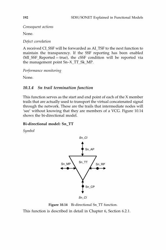
Consequent actions

None.

Defect correlation

A received CI_SSF will be forwarded as AI_TSF to the next function tomaintain the transparency. If the SSF reporting has been enabled(MI_SSF_Reported¼ true), the cSSF condition will be reported viathe management point Sn–X_TT_Sk_MP.


None.

10.1.4 Sn trail termination function

This function serves as the start and end point of each of the X membertrails that are actually used to transport the virtual concatenated signalthrough the network. These are the trails that intermediate nodes will‘see’ without knowing that they are members of a VCG. Figure 10.14shows the bi-directional model.

Bi-directional model: Sn_TT

Symbol

This function is described in detail in Chapter 6, Section 6.2.1.

Sn_TT

Sn_CP

Sn_AP

Sn_MP Sn_RP

Sn_CI

Sn_CI

Figure 10.14 Bi-directional Sn_TT function.


10.2 LCAS-CAPABLE VCAT FUNCTIONS

The LCAS-capable virtual concatenated Sn path layer functionalmodel is similar to the virtual concatenation model with the additionof the LCAS functionality. To make the distinction it will be referred toas Sn–Xv–L.

10.2.1 Sn–Xv–L layer trail termination function

The decomposition for this virtual concatenation function withLCAS enabled is almost the same as the one shown and described inSection 10.1 of this chapter. The Sn–Xv–L_TT function can be furtherdecomposed as depicted in Figure 10.15.

Sn-Xv-L Sn-Xv/Sn-X-L

Sn-X-L

Sn Sn

Sn-Xv_AI=

Sn_AI[1...X]

Sn_CI Sn_CISn-Xv_CI = Sn_CI[1...X]

Sn-X-L_AI

1 . . . . . . . X

Sn-X-L_AI

1 . . . . . . . . . X

Sn-X-L_CI

Sn-X-L/client Sn-X-L/client

<client>_CI<client>_CI

X = XM

X = XM

XA

XA

Sn-X-L_AP

Sn-X-L_AP

CP CP

Sn_CP Sn_CP

Sn_AP

Sn-X-L_CP

XA

Figure 10.15 Decomposition of Sn-Xv-L_TT function.


Note the following technology-specific particularizations:

� The Sn–Xv/Sn–X–L_A adaptation function contains LCAS specificprocesses.

� The Sn–X–L_TT termination function contains LCAS specific pro-cesses.

� The maximum value of X, i.e. XM, or XMT for the transmit side andXMR for the receive side, is technology specific, e.g. X¼ 64 for S12.The number of members that are actually carrying payload or theactive members is XA.

10.2.2 Sn–Xv/Sn–X–L adaptation function

This is the function that performs the adaptation of the (conti-guous concatenated) client signal to the (virtual concatenated)server layer signals transported by the members of the VCG. Anindication of the available transport bandwidth (XA) is senttowards the client layer. Figure 10.16 shows the bi-directionalmodel.

Bi-directional model: Sn–Xv/Sn–X–L_A

Symbol

This model can be further decomposed into the uni-directional sourceand sink atomic models (Figures 10.17 and 10.19).

Sn-Xv/Sn-X-L_A

1 . . . . . . X X = XM

Sn-Xv/SnX-L_A_MP Sn-Xv/Sn-X-L_RP

Sn-X-L_CP

Sn-Xv_AP

XA

Sn-Xv/SnX-L_A_MI Sn-Xv/Sn-X-L_RI

Sn-X-L_CI


Figure 10.16 Bi-directional Sn-Xv/Sn-X-L_A function.


Source side: Sn–Xv/Sn–X–L_A_So

Symbol

Interfaces

Processes

The process definitions for this function are the same as for theSn–Xv/Sn–X_A_So function described in Section 10.1.2, when the LCAScapability is enabled (MI_LCASEnable¼ true), with the following

Sn-Xv/Sn-X-L_A_So

1 . . . . . . XX = XMT

Sn-Xv/SnX-L_A_So_MP Sn-Xv/Sn-X-L_RP

Sn-X-L_So_CP

Sn-Xv_So_AP

XAT

Sn-Xv/SnX-L_A_So_MI Sn-Xv/Sn-X-L_RI

Sn-X-L_CI

Sn-Xv_AI = S n_AI[1...X]

Figure 10.17 Source side Sn-Xv/Sn-X-L_A function.

Sn–Xv/Sn–X–L_A_So.

inputs outputs

at Sn–X–L_So_CP at Sn–X–L_So_CP

Sn–X–L_CI_D Sn–X–L_CI_XAT

Sn–X–L_CI_CKSn–X–L_CI_FS

at Sn–Xv_So_AP

Sn_AI[1. . .X]_DSn_AI[1. . .X]_CKSn_AI[1. . .X]_FS

at Sn–Xv/Sn–X–L_A_So_MP at Sn–Xv/Sn–X–L_A_So_MP

Sn–Xv/Sn–X–L_A_So_MI_LCASEnable Sn–Xv/Sn–X–L_A_So_MI_XAT

Sn–Xv/Sn–X–L_A_So_MI_ProvM[1. . .X] Sn–Xv/Sn–X–L_A_So_MI_XMT

Sn–Xv/Sn–X–L_A_So_MI_PLCTThr Sn–Xv/Sn–X–L_A_So_MI_TxSQ[1. . .X]Sn–Xv/Sn–X–L_A_So_MI_cPLCTSn–Xv/Sn–X–L_A_So_MI_cTLCTSn–Xv/Sn–X–L_A_So_MI_cFOPT

at Sn–Xv/Sn–X–L_RPSn–Xv/Sn–X–L_RI_RS_Ack_recSn–Xv/Sn–X–L_RI_RS_Ack_genSn–Xv/Sn–X–L_RI_MST_rec[0. . .(max)]Sn–Xv/Sn–X–L_RI_MST_gen[0. . .(max)]


technology-specific particularizations:

� determines whether the payload size of the VCG matches the sizeof the client signal;

� determines the provisioned size XPT of the VCG and the maximumVCG size XMT; each member is provisioned (MI_ProvM[i]) to be amember of the group;

� determines the actual size XAT of the VCG; the number of active, i.e.payload transporting, members;

� determines which members are (temporarily) failed;� provides a temporary VCG size reduction, and hitless addition of a

previously failed member in coordination with the sink function;� provides a hitless increase and decrease of the VCG XAT, coordi-

nated with the sink function;� inserts the VCAT overhead information in each of the VCG member

signals, i.e. VCG identification, multi-frame indication, sequence num-ber, acknowledge, member status and CRC; the SQ number assignedto each member is available as TcSQ at the management point.

A detailed description of the processes is provided in ITU-T Rec.G.806 (2004) clause 10.1. The processes described above and theirrelations are depicted in Figure 10.18.

Sn-Xv_AP

Sn-X_CP

AI_

D

C2

distribution: octet by octet

CI_

D

payl

oad

PO

H

payl

oad

PO

H

VC

AT

-LC

AS

AI_

D

AI_

D

payl

oad

PO

H

1 2 .....................X

SQ assignment

SQ=0 1 .................... X-1

CI_

AA

T

MI_AAT

MI_AMT

MI_TxSQ

MI_cPLCTMI_cTLCTMI_cFOP

Sn

-Xv/

Sn-

X_A

_So

_MP

MI_LCASEnableMI_ProvM[i]MI_PLCTThr

RI_RS_Ack_recRI_MST_rec

RI_RS_Ack_genRI_MST_gen

Sn-Xv/Sn-X-L_RP

Figure 10.18 Sn-Xv/Sn-X-L_A_So processes.


Defects

Unexpected persistent member status MST shall be detected.

Consequent actions

None.

Defect correlation

The following probable causes are detected and reported by thedistribution process:

� If the LCAS procedure receives unexpected events the process maybe in the wrong state; this is reported as Failure Of Protocol Transmit(FOPT).

� If one or more members is removed temporarily from the VCGdue to a network problem, a Partial Loss of payload Capacity Trans-mit (PLCT) may be reported; a threshold (MI_PLCTThr) can beset.

� If all members in the VCG are removed temporarily, a Total Loss ofpayload Capacity Transmit (TLCT) is reported.


None.

Sink side: Sn–Xv/Sn–X–L_A_Sk

Symbol

Sn-Xv/Sn-X-L_A_Sk

1 . . . . . . XX = XMR

Sn-Xv/SnX-L_A_Sk_MP Sn-Xv/Sn-X-L_RP

Sn-X-L_Sk_CP

Sn-Xv_Sk_AP

XAR

Sn-Xv/SnX-L_A_Sk_MI Sn-Xv/Sn-X-L_RI

Sn-X-L_CI


Figure 10.19 Sink side Sn-Xv/Sn-X-L_A function.


Interfaces

Processes

The process definitions for this function are the same as for the Sn–Xv/Sn–X_A_Sk function described in Section 10.1.2, if MI_LCASEnable¼true, with the following technology-specific particularizations:

� determines if the received VCG payload size will fit in the clientsignal;

� determines the provisioned size XPR and maximum size XMR of theVCG; each member is provisioned (MI_ProvM[i]) to be a memberof the group;

Sn–Xv/Sn–X–L_A_Sk.

inputs outputs

at Sn–Xv_Sk_AP at Sn–X–L_Sk_CP

Sn_AI[1. . . X]_D Sn–X–L_CI_D

Sn_AI[1. . . X]_CK Sn–X–L_CI_CK

Sn_AI[1. . . X]_FS Sn–X–L_CI_FS

Sn_AI[1. . . X]_TSF Sn–X–L_CI_SSF

Sn_AI[1. . . X]_TSD Sn–X–L-CI_XAR

at Sn–Xv/Sn–X–L_A_Sk_MP at Sn–Xv/Sn–X–L_A_Sk_MP

Sn–Xv/Sn–X–L_A_Sk_MI_ProvM[1. . . X] Sn–Xv/Sn–X–L_A_Sk_MI_XMR

Sn–Xv/Sn–X–L_A_Sk_MI_LCASEnable Sn–Xv/Sn–X–L_A_Sk_MI_XAR

Sn–Xv/Sn–X–L_A_Sk_MI_PLCRThr Sn–Xv/Sn–X–L_A_Sk_MI_DMFI[1. . .M]

Sn–Xv/Sn–X–L_A_Sk_MI_TSDEnable Sn–Xv/Sn–X–L_A_Sk_MI_LCAS_So_Detected

Sn–Xv/Sn–X–L_A_Sk_MI_HOTime Sn–Xv/Sn–X–L_A_Sk_MI_cPLCR

Sn–Xv/Sn–X–L_A_Sk_MI_WTRTime Sn–Xv/Sn–X–L_A_Sk_MI_cTLCR

Sn–Xv/Sn–X–L_A_Sk_MI_cFOPR

Sn–Xv/Sn–X–L_A_Sk_MI_cLOM[1. . . X]

Sn–Xv/Sn–X–L_A_Sk_MI_cSQM[1. . .M]

Sn–Xv/Sn–X–L_A_Sk_MI_cMND[1. . .M]

Sn–Xv/Sn–X–L_A_Sk_MI_AcSQ[1. . .M]

Sn–Xv/Sn–X–L_A_Sk_MI_cPLM[1. . .M]

Sn–Xv/Sn–X–L_A_Sk_MI_AcSL[1. . .M]

at Sn–Xv/Sn–X–L_RP

Sn–Xv/Sn–X–L_RI_RS_Ack_rec

Sn–Xv/Sn–X–L_RI_RS_Ack_gen

Sn–Xv/Sn–X–L_RI_MST_rec[0. . .(max)]

Sn–Xv/Sn–X–L_RI_MST_gen[0. . .(max)]


� determines the actual size XAR of the VCG; the number of active, i.e.payload transporting, members;

� determines which VCG members are (temporarily) failed;� provides a temporary group size reduction, and supports hitless

addition of a previously failed signal in coordination with thesource function. The reduction may be based on degraded signalsif MI_TSDEnable¼ true; the reduction can be postponed (hold-off)by time MI_HOTime and the addition (wait to restore) by timeMI_WTRtime;

� provides a hitless increase and decrease of the active group XAR,coordinated with the source function.

A detailed description of the processes is provided in ITU-T Rec.G.806 (2004) clause 10.1. The processes described above and theirrelations are depicted in Figure 10.20.

Sn-Xv_AP

Sn-X_CP

AI_

D

C2

assembly: octet by octet

CI_

D

pay

loa

d

PO

H

pay

loa

d

PO

H

VC

AT

-LC

AS

AI_

D

AI_

D

pay

loa

d

PO

H

1 2 .....................X

re-alignment / re-order

SQ=0 1 .................... X-1

CI_

AA

R

MI_AAR

MI_AMR

MI_AcSQ[i]MI_cFOPRMI_cTLCRMI_cPLCRMI_cLOM[i]MI_cSQM[i]MI_cMND[i]MI_DMFI[i]MI_LCAS_So_Det

Sn

-Xv/

Sn-

X_A

_So

_MP

RI_MST_genRI_RS_Ack_genRI_MST_recRI_RS_Ack_rec

MI_PLCRThrMI_ProvM[i]MI_LCASEnableMI_TSDEnableMI_HOTimeMI_WTRTime

buffer bufferbuffer

MI_cPLM[i]MI_AcSL[i]MI_cLOA

Sn-Xv/Sn-X-L_RP

Figure 10.20 Sn-Xv/Sn-X-L_A_Sk processes.


Defects

The following defects will be detected and reported:

� Loss of Multi-frame (dLOM) if the LCAS overhead cannot berecovered or aligned between members;

� Inconsistent sequence numbering (dSQNC);� Member Not De-skewable (dMND) if the differential delay is too large

for the buffers;� Persistent CRC errors (dCRC).

Consequent actions

The consequent action is the maintenance signal Member ServiceUnavailable—LCAS active (mMSU–L) if either a signal fail is receivedfrom a member Sn_TT, or a LOM or an MND is detected. Conse-quently, the output signal is replaced by an AIS signal together with anSSF indication.

Defect correlation

Determines the most probable causes cLOM, cMND, cLOA, cSQM,cPLCR, cTLCR, cFOPR. The latter three causes are similar to cPLCT,cTLCT and cFOPT in the source function.


None.

10.2.3 Sn–X–L trail termination function

This function serves as the start and end point of the virtualtrail that is used to transport the virtual concatenated signalthrough the network. If LCAS is enabled the payload size of thevirtual trail can vary. The bi-directional model is shown inFigure 10.21.


Bi-directional model: Sn–Xv/Sn–X_So_A

Symbol

This model can be further decomposed into the uni-directional sourceand sink models (see Figures 10.22 and 10.23).

Source side: Sn–X–L_TT_So

Symbol

Sn-X-L_TT

Sn-X-L_AI

Sn-X-L_CP

Sn-X-L_TT_MI

Sn-X-L_AP

Sn-X-L_CI

Sn-X-L_TT_MP

XA

XA

Figure 10.21 Bi-directional Sn-X-L_TT function.

Sn-X-L_TT_So

Sn-X-L_AI

Sn-X-L_So_CP

Sn-X-L_So_AP

Sn-X-L_CI

XAT

XAT

Figure 10.22 Source side Sn-X-L_TT function.


Interfaces

Processes

The process definitions for this function are the same as for theSn–X_TT_So function described in Section 10.1.3 with the followingtechnology-specific particularization:

� The number of active members XAT in the VCG received fromthe Sn–Xv/Sn–X–L_A_So function is transferred back to theSn–X–L/client_A_So function for transparency.

Defects

None.

Consequent actions

None.

Defect correlation

None.


None.

Sn–X–L_TT_So.

inputs outputs

at Sn–X–L_So_AP at Sn–X–L_So_APSn–X–L_AI_D Sn–X–L_AI_XAT

Sn–X–L_AI_CKSn–X–L_AI_FS

at Sn–X–L_So_CP at Sn–X–L_So_CPSn–X–L_CI_XAT Sn–X–L_CI_D

Sn–X–L_CI_CKSn–X–L_CI_FS


Sink side: Sn–X–L_TT_Sk

Symbol

Interfaces

Processes

The process definitions for this function are the same as for theSn–X_TT_Sk function described in Section 10.1.3 with the followingtechnology-specific particularizations:

� The number of active members XAR in the VCG received fromthe Sn–Xv/Sn–X–L_A_Sk function is transferred to the Sn–X–L/client_A_Sk function.

Defects

None.

Sn-X-L_TT_Sk

Sn-X-L_AI

Sn-X-L_Sk_CP

Sn-X-L_TT_Sk_MI

Sn-X-L_Sk_AP

Sn-X-L_CI

Sn-X-L_TT_Sk_MP

XAR

XAR

Figure 10.23 Sink side Sn-X-L_TT function.

Sn–X–L_TT_Sk.

inputs outputs

at Sn–X–L_Sk_CP at Sn–X–L_Sk_APSn–X–L_CI_D Sn–X–L_AI_DSn–X–L_CI_CK Sn–X–L_AI_CKSn–X–L_CI_FS Sn–X–L_AI_FSSn–X–L_CI_SSF Sn–X–L_AI_TSFSn–X–L_CI_XAR Sn–X–L_AI_XAR

at Sn–X–L_TT_Sk_MP at Sn–X–L_TT_Sk_MPSn–X–L_TT_Sk_MI_SSF_Reported Sn–X–L_TT_Sk_MI_cSSF


Consequent actions

aTSF CI SSF

Defect correlation

cSSF CI SSF and SSF Reported


None.

10.2.4 Sn trail termination function

See Section 10.1.3 for the description. This function does not have anyLCAS specific functionality. However, because LCAS is per definitionasymmetrical, the member trails are uni-directional and hence RDIand REI are not supported when LCAS is enabled.

10.2.5 Sn–X–L to client signal adaptation function

This function requires client specific inputs, outputs and processes. Itis included here to show that the XAT and XAR signals received fromthe VCG adaptation function have to be processed by this function toadjust the client signal to the available bandwidth. Figure 10.24 showsthe bi-directional model of this adaptation function.

Bi-directional model: Sn–X–L/<client>_A

Symbol

Sn-X-L/<client>_A

Sn-X-L_AP

<client>_CI

<client>_CP

Sn-X-L_AI

XA

Sn-X-L/<client>_A_MI

Sn-X-L/<client>_A_MP

Figure 10.24 Bi-directional Sn-X-L/<client>_A function.


This model can be further decomposed into the uni-directional modelsof the source and sink side (see Figures 10.25 and 10.26).

Source side: Sn–X–L/<client>_A_So

Symbol

Interfaces

Processes

The process has the following technology-specific particularizations:

� The incoming client signal is mapped into the payload area of theSn–X–L signal. The number of active members XAT determines theavailable payload size. XAT is received from the Sn–Xv/Sn–X–L_A_So function via the VCG Sn–X–L_TT_So function.

Sn-X-L/<client>_A_So

Sn-X-L_So_AP

<client>_CI

<client>_So_CP

Sn-X-L_AI

XAT

Sn-X-L/<client>_A_So_MI

Sn-X-L/<client>_A_So_MP

Figure 10.25 Source side Sn-X-L/<client>_A function.

Sn–X–L/<client>_A_So.

inputs outputs

at Sn–X–L_So_AP at Sn–X–L_So_APSn–X–L_XAT Sn–X–L_D

Sn–X–L_CKSn–X–L_FS

at <client>_So_CP at <client >_So_CP<client>_CI_nn client>_CI_nn

at Sn–X–L/ <client>_A_So_MP at Sn–X–L/ <client> _A_So_MPSn–X–L/<client>_A_So_MI_nn Sn–X–L/<client>_A_So_MI_nn


Defects

None.

Consequent actions

None.

Defect correlation

None.


None.

Sink side: Sn–X–L/<client>_A_Sk

Symbol

Interfaces

Sn-X-L/<client>_A_Sk

Sn-X-L_Sk_AP

<client>_CI

<client>_Sk_CP

Sn-X-L_AI

XAR

Sn-X-L/<client>_A_Sk_MI

Sn-X-L/<client>_A_Sk_MP

Figure 10.26 Sink side Sn-X-L/<client>_A function.

Sn–X–L/<client>_A_Sk.

inputs outputs

at Sn–X–L_Sk_APSn–X–L_DSn–X–L_CKSn–X–L_FSSn–X–L_TSFSn–X–L_XAR

at < client >_Sk_CP at < client >_Sk_CP<client>_CI_nn <client>_CI_nn


Processes

The process has the following technology-specific particularizations:

� The outgoing client signal is retrieved from the payload area ofthe Sn–X–L signal. The number of active members XAT deter-mines the actual payload size. XAT is received from the VCGfunction Sn–Xv/Sn–X–L_A_Sk transferred by the Sn–X–L_TT_Skfunction.

VC–n specific sink process

C2: The signal label is recovered from the C2 byte as per ITU-T Rec.G.806 (2004) clause 6.2.4.2. The signal label value ‘<client> layermapping’ shall be expected. The accepted value of the signal labelAcSL is also available at the Sn–X–L/ETH_A_Sk_MP.

Defects

dPLM and <client> layer specific defects.

Consequent actions

<client> layer specific consequent actions.

Defect correlation

cPLM and <client> layer specific probable causes.


<client> layer specific.

10.3 VCAT NETWORK MODEL

Figure 10.27 depicts an example functional model of a virtual con-catenation sub-layer network illustrating the transport of a single

at Sn–X–L/< client >_A_Sk_MP at Sn–X–L/ < client > _A_Sk_MPSn–X–L/<client>_A_Sk_MI_Active Sn–X–L/<client>_A_Sk_MI_cPLMSn–X–L/<client>_A_Sk_MI_nn Sn–X–L/<client>_A_Sk_MI_AcSL

Sn–X–L/<client>_A_Sk_MI_nn


contiguous client signal <client>_CI in a group of X individualmember signals Sn_CI. Whether LCAS is enabled or disabled isirrelevant for this model. For simplicity only two member networkconnections are shown. Diverse routing is illustrated by the differentsub-network connections in the Sn layer network for the intermediatenodes. The compound functions ‘srv’ represent the adaptation andtermination of the server layer that is used to support the X individualmember network connections Sn_NC[i].

10.4 S4–Xc TO S4–Xc INTERWORKING FUNCTION

Contiguous concatenated characteristic information Sn–Xc_CI andvirtual concatenated characteristic information Sn–Xv_CI do haveexactly the same payload capacity if they have the same index X.The adapted information of both signals is the same: Sn–X_AI. Thisfeature enabled the deployment of an application specific compoundfunction—the Sn–Xc to Sn–Xv interworking function—a feature that

srv

Sn-X trail

Sn-X/<client>

Sn-Xv

srv

Sn-X/<client>

Sn-Xv

srv srv

srv srv

srv

srv

<server> NC <server> NC

Sn NC[X]

Sn NC[1]

SNC SNCSNC

SNC

Sn-X_AP

Sn_CP

Sn_TCP

Sn sub-network


Sn_CI

Figure 10.27 Example of a VCAT network connection.


provides a new possibility for layer network interworking. A specialsymbol has been defined for this function that provides the transfor-mation between contiguous concatenation and virtual concatenation:the interworking function. The application is limited to concatenatedS4 signals; more specifically X is limited to the values 4, 16, 64 and 256.The symbol that has been defined for the interworking function isdepicted in Figure 10.28.

This function can be decomposed into the following atomic func-tions: the virtual concatenation trail termination function Sn–Xv_TTand the contiguous concatenation trail termination function Sn–Xc_TT.Figure 10.29 illustrates the decomposition. For a description of the

S4_CI[1...X]S4-Xc_CP

1...

X

S4-Xc <> S4-Xv

S4-Xc>S4-Xv_I_MI

S4-Xv_CP

S4-Xc>S4-Xv_I_MP

S4-Xc_CI

Figure 10.28 S4-XC<>S4-Xv compound function.

Sn-Xv


Sn-X_AI

1 . . . . . . . X

Sn-Xc_CI

Sn-Xc_CP

Sn-X_AP

Sn_CP

Sn-Xc

S4-Xc <> S4-Xv

1 . . . . . . . X Sn_CP

Sn-Xc_CP

Sn-Xc_CI


Figure 10.29 Decomposition of the Sn-Xv<>Sn-Xc function.


Sn–Xv_TT function, see Section 10.1. The description of the Sn–Xc_TTfunction is similar to that of the Sn_TT function described in Sec-tion 10.1.4 because the only difference is the size of the payload area ofthe terminated signal, i.e. it is X times the size of an Sn structure.

The following sections describe the functionality of the interworkingfunction starting with the bi-directional model in Figure 10.30.

Bi-directional model: Sn–Xc <> Sn–Xv

This model can be further decomposed into the contiguous-to-virtualinterworking function (Figure 10.31), and the virtual-to-contiguousinterworking function (Figure 10.33).

Contiguous to virtual: S4–Xc > S4–Xv_I

Symbol

This uni-directional interworking function will convert a contiguousconcatenated signal S4–Xc_CI into a virtual concatenated signalS4–Xv_CI that is equivalent to X individual signals S4_CI. Currently,values of X¼ 4, 16, 64 and 256 are allowed.


1...

X

S4-Xc <> S4-Xv

S4-Xc>S4-Xv_I_MI

S4-Xv_CP

S4-Xc>S4-Xv_I_MP

S4-Xc_CI

Figure 10.30 Bi-directional S4-Xc<>S4-Xv model.


1...

X

S4-Xc > S4-Xv

S4-Xc>S4-Xv_I_MI

S4-Xv_CP

S4-Xc>S4-Xv_I_MP

S4-Xc_CI

Figure 10.31 S4-Xc>S4-Xv interworking function.


Interfaces

Processes

� The received TTI in the S4–Xc overhead will either be sent inthe overhead of all S4s of the S4–Xv or only in the overhead ofthe first S4 of the S4–Xv. In the latter case (if provisioned TIEn¼true) the TTI of the remaining S4s has to be provisioned by theNMS.

� The number of bit errors detected in the S4–4c signal will be addedto the BIP calculated before insertion in the first S4 (SQ¼ 0) of theS4–4v. For the remaining S4s of the S4–Xv the BIP is calculated andinserted without change.

� The signal label of the S4–Xc will be inserted in the overhead of allindividual S4s of the S4–Xv signal.

� The REI of the S4–Xc will be inserted in the first S4 of the S4–Xv.The REI of all other S4s of the S4–Xv will be set to 0.

� The RDI of the S4–Xc will be inserted in all S4s of the S4–Xv.� If the Tandem Connection (TC) Overhead (TCOH) bits 1 to 4, the

Incoming Error Count (IEC), of the S4–Xc contain the code ‘1110’(Incoming AIS), the TCOH bits 1 to 4 of all S4s of the S4-v will be setto ‘1110’. If the IEC of the S4–Xc contains the code ‘0000’ (part of TCUnequipped), the IEC of all S4s of the S4–Xv will be set to ‘0000’.Otherwise, the IEC of the S4–Xc will be copied to the IEC of the firstS4 of the S4–Xv and the IEC of all other S4s of the S4–Xv shall be setto an ‘1001’ indicating IEC¼ 0. The TC Overhead bits 5 to 8 will beinserted in the first S4 of the S4–Xv. The TCOH bits 5 to 8 of allother S4s of the S4–Xv will be set to 0.

S4–Xc>S4–Xv_I.

inputs outputs

at S4–Xc_CP at S4–Xv_CPS4–Xc_CI_D S4_CI[1. . . X]_DS4–Xc_CI_CK S4_CI[1. . . X]_CKS4–Xc_CI_FS S4_CI[1. . . X]_FSS4–Xc_CI_SSF S4_CI[1. . . X]_SSF

at S4–Xc>S4–Xv_I_MIS4–Xc>S4–Xv_I_MI_TIEnS4–Xc>S4–Xv_I_MI_TxTI[2. . . X]


� The remaining overhead bytes of the S4–Xc will be inserted in thefirst S4 of the S4–Xv signal. The remaining overhead bytes of allother S4s of the S4–Xv will be set to 00h.


Defects

None.

Consequent actions

A received SSF will be sent as SSF on all S4s of the S4–Xv and thesignal of all S4s is replaced by AIS.

aAIS CI SSF

aSSF½n� CI SSF

Defect correlation

None.


None.

Sn-Xv_CP

Sn-Xc_CPA

I_D

payloadC

I_D

payl

oad

PO

H

payl

oad

PO

H

OH

inte

rwor

king

AI_

D

AI_

D

payl

oad

PO

H

1 2 .....................X

PO

H

distribution octet by octet

Figure 10.32 Sn-Xc>Sn-Xv processes.


Virtual to contiguous: S4–Xv>S4–Xc_I

Symbol

This uni-directional interworking function will convert a virtual con-catenated signal S4–Xv_CI transported by X individual signals S4_CIinto a contiguous concatenated signal S4–Xc_CI. Currently, values ofX¼ 4, 16, 64 and 256 are allowed.

Interfaces

S4-Xv_CI=

S4_CI[1...X]

S4-Xc_CP1....X

S4-Xv > S4-Xc

S4-Xv>S4-Xc_I_MI

S4-Xc_CI

S4-Xv>S4-Xc_I_MPS4-Xv_CP

Figure 10.33 Sink side S4-Xv>S4-Xc function.

S4–Xv>S4–Xc_I.

inputs outputs

at S4–Xv_CP at S4–Xc_CPS4_CI[1. . . X]_D S4–Xc_CI_DS4_CI[1. . . X]_Ck S4–Xc_CI_CKS4_CI[1. . . X]_FS S4–Xc_CI_FSS4_CI[1. . . X]_SSF S4–Xc_CI_SSF

at S4–Xc>S4–Xv_I_MI at S4–Xc>S4–Xv_I_MIS4–Xv>S4–Xc_I_MI_Tpmode S4–Xv>S4–Xc_I_MI_cTIM[1. . . X]S4–Xv>S4–Xc_I_MI_SSF_Reported S4–Xv>S4–Xc_I_MI_cUNEQ[1. . . X]S4–Xv>S4–Xc_I_MI_ExTI[1. . . X] S4–Xv>S4–Xc_I_MI_cSSF[1. . . X]S4–Xv>S4–Xc_I_1second S4–Xv>S4–Xc_I_MI_AcTI[1. . . X]S4–Xv>S4–Xc_I_TIMdis[1. . . X] S4–Xv>S4–Xc_I_MI_cLOM[1. . . X]

S4–Xv>S4–Xc_I_MI_cSQM[1. . . X]S4–Xv>S4–Xc_I_MI_cLOAS4–Xv>S4–Xc_I_MI_AcSQ[1. . . X]


Processes

The following processes are performed per individual S4 in the S4–Xv:

� The TTI is recovered from S4 overhead. The accepted value isreported as AcTI and it is compared to the provisioned expected(ExTI) value. A detected mismatch defect (dTIM) is reported (cTIM)if the reporting is not disabled (TIMdis). (Note: If no individualTTIs are configured for the S4s in the S4–Xc>S4–Xv_I function, theexpected TTI for all S4s has to be set equal to the expected TTI ofthe first S4, or TPmode has to be set for these S4[2. . .(X� 1)].)

� The signal label byte C2 will be recovered. It will be used to detect(dUNEQ) and report (cUNEQ) the unequipped defect or the AIScondition (dAIS).

� The SQ will be recovered and after acceptation it will be reported asAcSQ. A new sequence number is accepted if it has m times thesame value with 3 � m � 10.

The following functions will be performed for the S4–Xc:

� The H4 byte of the S4–Xc will be set to ‘0’.� The received TTI of the first S4 of the S4–Xv shall be inserted to the

S4–Xc.� The BIP–8 will be calculated for each S4 frame of the S4–Xv and

compared with the related received BIP–8 to determine the biterrors per S4. The bit errors of all S4s of the S4–Xc will be addedtogether and the result will be added to the BIP–8 calculated forS4–Xc frame. The resulting BIP–8 will be inserted in the S4–Xcoverhead.

� The signal label of the first S4 of the S4–Xv shall be inserted in theS4–Xc.

� The REI values of all S4s of the S4–Xv will be added together. Theresult will be inserted in the S4–Xc.

� If the RDI of any S4 of the S4–Xv is set, the RDI of the S4–Xc shall beset to ‘1’.

� If the TCOH bits 1 to 4 (IEC) of any S4 of the S4–Xv contain the code‘1110’ (Incoming AIS), TCOH bits 1 to 4 of the S4–Xc shall be set to‘1110’. If the IEC of the first S4 of the S4–Xv contain the code ‘0000’(TC Unequipped), the IEC of the S4–Xc shall be set to ‘0000’.Otherwise, the IEC values of all S4s of the S4–Xv will be addedtogether and inserted as IEC in the S4–Xc. TCOH bits 5 to 8 of thefirst S4 of the S4–Xv will be copied to TCOH bits 5 to 8 of the S4–Xc.


The remaining overhead bytes of the first S4 of the S4–Xv will becopied to the S4–Xc. The processes described above and their relationsare depicted in Figure 10.34.

Defects

For each individual VC–4, the defects dUNEQ, dAIS and dTIM shallbe detected as described above.

After re-aligning by using the multi-frame process, and re-orderingby using the re-sequence process, the X individual VC–4s the follow-ing defects are detected for the VCG:

� Loss Of Multi-frame (dLOM): The VCAT overhead multi-framecannot be recovered from the received signal.

� Sequence number Mismatch (dSQM): The accepted SQ number (AcSQ)of a member does not match the expected SQ number (EcSQ). Theexpected SQ number of member p in a VCG is (p� 1).

� Loss of Alignment (dLOA): The differential delay, i.e. the differencein time between the member experiencing the least propagation

Sn-Xv_CP

Sn-Xc_CP

AI_

D

payload

CI_

D

payl

oad

PO

H

payl

oad

PO

H

OH

inte

rwor

king

AI_

D

AI_

D

payl

oad

PO

H

1 2 .....................X

PO

H

buffer bufferbuffer MI_cLOA

MI_cTIM[i]MI_AcTI[i]MI_cUNEQ[i]MI_AcSQ[i]MI_cSSF[i]MI_cSQM[i]MI_cLOM[i]

Sn-

Xv/

Sn

-X_A

_So

_MP

MI_TPmodeMI_ExTI[i]MI_TIMdis[i]MI_1_secondMI_SSF_Reported

SQ=0 1 .....................X-1

assembly octet by octet

re-align / re-order

Figure 10.34 Sn-Xv>Sn-Xc processes.


delay and the member experiencing the most propagation delay inthe network, exceeds the implemented alignment buffer.

Consequent actions

If one of the defects dTIM, dLOM, dSQM or dLOA is detected, theS4–Xc signal will be replaced by an AIS signal.

Defect correlation

Based on the detected defects this process will determine the mostprobable causes: cUNEQ, cTIM, cSSF, cLOM, cSQM and cLOA.


None.

10.5 VCAT-CCAT INTERWORKING NETWORK MODEL

The Sn–Xc <> Sn–Xv compound function defined in ITU-T Re. G.805(2000) is located between an Sn–Xc and an Sn–Xv layer network with

srv

Sn-X trail

Sn-X/<client>

Sn-Xv

srv

Sn-X/<client>

Sn-Xc

srv

srv srv srv

server NC

server NC

SNC SNCSNCSNC

Sn-X_AP

Sn_CP

Sn_TCPSnnetwork

Sn-Xcnetwork

Sn-

Xv

Sn-

Xc

< >

Sn-Xc_TCP


Sn-Xc_CP

Figure 10.35 Example of VCAT CCAT network interworking.


the same index X, where the latter is in fact an Sn layer network with Xseparate Sn sub-network connections. Figure 10.35 shows an examplefunctional network architecture illustrating the transport of a contig-uous client signal <client>_CI over a network, partly as a virtualconcatenated signal and partly as a contiguous concatenated signal.The interworking processing function performs the semantically‘transparent’ conversion of the virtual concatenation trail overheadto contiguous concatenation trail overhead and vice versa. An Sn–Xtrail may contain one or more interworking processing functions. Thecompound functions ‘srv’ represent the adaptation and termination ofthe server layer that is used to support the transport of the Xindividual member signals Sn_CI[i] or the single contiguous concate-nated signal Sn–Xc_CI.


11

Example functional modelsto exercise

In this chapter a number of examples are provided to illustrate the use offunctional modeling at different levels in the network. They include themodel used by a device implementer, a model used by a unit leveldesigner, a network element description, and a network application.

A functional model can be read best if it is drawn on a single page orsheet. This can be achieved, without losing the required overall func-tionality, by using compound functions, and/or by removing sublayers,e.g. protection sublayers or performance monitoring sublayers, andproviding separated figures containing the detailed sublayer informa-tion. The compound functions can be expanded to explain or describecertain detailed aspects of a functional model in separate figures.

11.1 DEVICE LEVEL FUNCTIONAL MODEL

In the first example, the most detailed functional model is providedcontaining all possible mappings of a 2.048 kbit/s PDH signal into aVC–12 container. Also, it includes a suggestion for a compoundfunction that can be used in less detailed functional models of a unitlevel or system level description.

Figure 11.1 shows a very detailed model of the functions that arepresent between the physical 2.048 kbit/s interface signal and theVC–12 signal. A detailed description of the atomic functions used inthis figure is given in ITU-T Rec. G.705 (2000).


E12/P12s_A

TTE12-Z

S12/P12x_A

P12s/P0-31cA

P12sTT

AP12s/P0-31c

TTP12s

P12_CPP12s_CP

P12x_CP

S12TT

E12/P12x_A

S12/P12s_A

E12

S12

P0-31c_C

S12/P0-31cA

P12s_C

P12s_C

E12_TCP

S12_TCP

E12_TCP

S12_TCP

P12

x_C

I

P12

s_C

I

P0-

31c_

CI

P12smTT

TTP12sm

Figure 11.1 Detailed 2Mbit/s model and compound representation.


The 2.048 kbit/s PDH or E12 characteristic information present atthe connection point E12_TCP is described in ITU-T Rec. G.703 (1998)clause 9. It is terminated in the E12-Z_TT function where Z indicatesthe supported cable impedance, 75� or 120�. Now, the recovered2.048 kbit/s signal can either be transported as a constant bitrate signal(disregarding any possible framing) or as an ITU-T Rec. G.704 (1998)or G.706 (1991) framed signal. This is shown by the presence of twoadaptation functions: E12/P12x_A and E12/P12s_A. The P12x_CIrepresents the CBR signal and P12s_CI represents the 32 octet basedframed signal. The S12/P12x_A provides a-synchronous (bit) mappingof the CBR signal in a VC–12 according to ITU-T Rec. G.707 (2003)clause 10.1.4.1. The S12/P12s_A provides byte synchronous (octet)mapping according to ITU-T Rec. G.707 (2003) clause 10.1.4.2.

A 2.048 kbit/s link may be partitioned into sections to improve faultlocalization and performance monitoring. In this case the framed2.048 kbit/s signal can be terminated in the P12s_TT function. Theremaining P0-31c_CI signal carries the 31 concatenated 64 kbit/s pay-load octets of the E12 signal at a total rate of 1984 kbit/s. This signalcan be mapped into a VC–12 according to ITU-T Rec. G.707 (2003)clause 10.1.4.3 in the S12/P0-31c_A function while using the perfor-mance information provided by the associated VC–12 for the sectioncarried through the SDH network. Also, it is possible to start imme-diately a new E12 section by adding again framing information to theP0-31c_CI signal in the P12s/P0-31c_A function and use byte synchro-nous mapping for transport of the signal in a VC–12. TheP12sm_TT_Sk monitors can be used to verify the performance of thetransported P12x_CI and P12s_CI signals, e.g. as required by a ServiceLevel Agreement (SLA).

This is the level of detail used by an implementer of this function-ality, e.g. a device designer or a software designer responsible forprovisioning.

If this level of detail is not required the model depicted in theshaded area of Figure 11.1 can replace the detailed model. It showstwo compound functions each existing of at least a terminationfunction and an adaptation function. The compound functions canbe used in a model to describe (parts of) equipment.

11.2 EQUIPMENT DETAILED FUNCTIONAL MODEL

In Chapter 3, Section 3.2, a description is provided of partitioningbased on the physical properties of a network and the capabilities of its

Example functional models to exercise 221

network elements. Partitioning can also be forced by the physicalproperties of the equipment itself. Figure 11.2 shows an example ofequipment partitioning. It illustrates how functions are groupedtogether, forced by the physical constraints. Here, the equipmentdimensions and internal and external connectivity determine thepartitioning of functions, e.g. the partitioned lower order connectionfunction S12_C or the electrical properties of the backplane. Theexpansion methodology described in Chapter 4, Section 4.2.3 hasbeen used to provide the internal, i.e. backplane, connectivity.

S4_TT

BT/S4_A

BT_TT

P12_CP

BT_TCP

S4/S12_A

S12_C

S4_TT

BT/S4_A

BT_TT

S4/S12_A

1 . . . . . . . . . . . x

E12

S12

E12

S12

S4_TT

BL/S4_A

BL_TT

S4/S12_A

BL/S4_A

BL_TT

BL_TCP

S4_C

MSnTT

RSnTT

RSn/MSnA

OSnTT

OSn/RSnA

MSn/S4A

Net

wor

k-U

nit

Cross-Connect-Unit

Trib

utar

y-U

nit

Backplane

S12_C

Figure 11.2 Example of an equipment model.


Depicted are three units that may exist in an add-drop multiplexer(ADM) and the backplane:

� a tributary unit that supports x individual 2.048 kbit/s PDH tribu-taries (E12) and a lower order (sub-network) connection function,providing, in this example, the lower order S12 connectivity;

� a cross-connect unit that supports the lower order and higher orderconnectivity required to provide the add/drop capability and thatalso takes care of connecting the through traffic;

� a network unit that supports an SDH interface for connecting theADM to the network;

� a backplane is used to interconnect all units and uses proprietary,implementation specific, backplane signals for tributary unitsBT_CI and network units BL_CI. These backplane signals requiretheir own specific adaptation and termination functions as shownin Figure 11.2 by the BT/S4_A, BT_TT, BL/S4_A and BL_TTsymbols.

A user who is interested only in the layer network topology willrepresent the VC–12 layer in this example network element asdepicted in Figure 11.3. In this abstract model one can identify the

tributary sub-networks with the ports representing the external inter-faces, the cross-connect sub-network without external ports and theconnecting links, i.e. the backplane connections. In this example, thebackplane connection has a VC–4 structure hence each link has acapacity to transport up to 63 VC–12s. A developer of the networkelement connection management application can use this abstract

VC-12 layer network

cross-connectsub-networklink

link

link

tributarysub-network



Figure 11.3 Abstract model representing a network element VC–12 layer.


model as a reference and will use the functional model to retrieve thedetailed information.

Even more partitioning is required when equipment protection isused to improve the availability of the system. In the example given inFigure 11.4, equipment protection has been provided by both doublingthe backplane signals and doubling a complete unit.

In this case the cross-connect unit is duplicated, i.e. a working unitand a protection unit are present in the system. This is similar to themethodology used for trail protection explained in Chapter 9, Section9.2.1. The connection functions Eq-P_C provide the protection switch-ing capability. The fact that an ADM requires two identical lineinterfaces can also be used in the partitioning of the system to provideequipment protection. In this case the cross-connect unit needsto support the MS trail protection methodology as described inChapter 9, Section 9.2.1.2. This is illustrated in Figure 11.5.

S12_C

S4_C

Cross-Connect-Unit_W

S4 S4

BT BL

1 . . . . . . . . x

E12

S12

E12

S12

Trib

utar

y-U

nit

Backplane

S12_C

S4

Eq-P_C

BTBT

OSn

RSn

MSn

BT

BT_TCP BL_TCP

Line

-Uni

t

S12_C

S4_C


S4 S4

BT BL

BL_TCP

BT

Eq-P_C

BT_TCP

Figure 11.4 Example 1 of an equipment model with equipment protection.


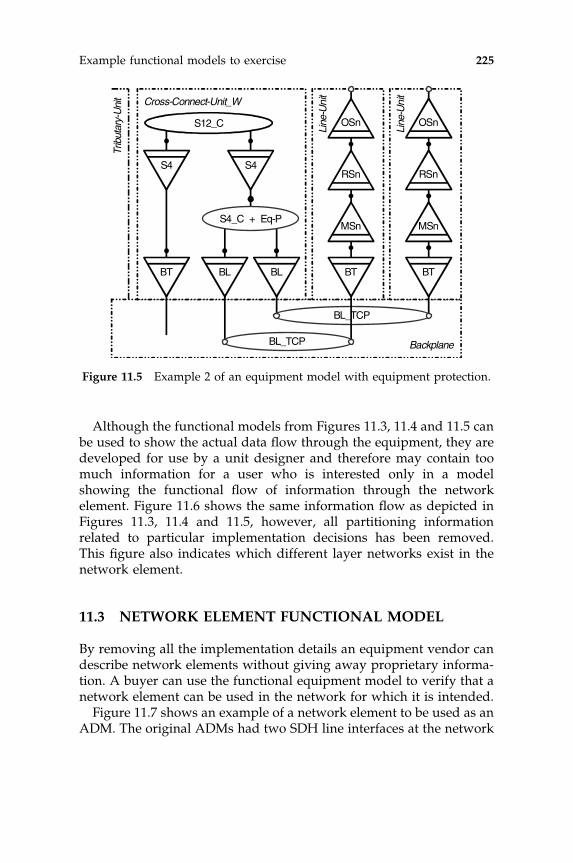
Although the functional models from Figures 11.3, 11.4 and 11.5 canbe used to show the actual data flow through the equipment, they aredeveloped for use by a unit designer and therefore may contain toomuch information for a user who is interested only in a modelshowing the functional flow of information through the networkelement. Figure 11.6 shows the same information flow as depicted inFigures 11.3, 11.4 and 11.5, however, all partitioning informationrelated to particular implementation decisions has been removed.This figure also indicates which different layer networks exist in thenetwork element.

11.3 NETWORK ELEMENT FUNCTIONAL MODEL

By removing all the implementation details an equipment vendor candescribe network elements without giving away proprietary informa-tion. A buyer can use the functional equipment model to verify that anetwork element can be used in the network for which it is intended.

Figure 11.7 shows an example of a network element to be used as anADM. The original ADMs had two SDH line interfaces at the network

Backplane

OSn

RSn

MSn

BT

Line

-Uni

t

S12_C

S4_C + Eq-P


S4 S4

BT BL BL

BL_TCP

OSn

RSn

MSn

BT

Line

-Uni

t

BL_TCP

Trib

utar

y-U

nit

Figure 11.5 Example 2 of an equipment model with equipment protection.


side and several PDH interfaces at the tributary side and also lowerorder SDH interfaces. If only one line interface is used or equipped thenetwork element is referred to as a Terminal Multiplexer (TM).

The maximum number of interfaces supported per tributary signalmay vary as indicated in Figure 11.7. The actual number of tributaryinterfaces depends on the number of available physical unit slots, thenumber of interfaces supported per unit and the connection capabil-ities of the lower order and higher order connection functions. Thismodel does not provide information about the protection capabilitiesof the ADM. If it is required to show the protection features, the

S12_C

S4_C

S4

lower orderconnection

function

MSn

RSn

OSn

S12E12

E12_TCPS12_TCP

S4_TCP

MSn_TCP

RSn_TCP

OSn_TCP

higher orderconnection

function

P12_CP

S12_CP

S4_CP

OS

nla

yer

RS

nla

yer

MS

nla

yer

S4

laye

r

S12

laye

r

E12

laye

r

P12

laye

r

Figure 11.6 Network element simplified functional model.


methodology described in Chapter 9, Section 9.2 (e.g. adding protec-tion layers) can be applied to extend the model.

An additional feature shown in this model is the support of TandemConnection Monitoring (TCM) indicated by the SnT compound functionand described in detail in ITU-T Rec. G.707 (2003) Annexes C and D.TCM provides performance monitoring of part(s) of a path, e.g. the partthat passes through a different operator domain (see also Chapter 8,

<lower order> Sm_C

<higher order> Sn_C

E12

S12

Eth

Sm-Xv

OS

RS

MS

E4

S4

Eth

Sm-Xv

Sn

RSn

[1...x] [1...a]

[1...z]

[1...b] [1...p] [1...q]

MSnMSn

OSn OSn

RSn

PDH Ethernet PDH

1 . . . . . . . . . . . . . . .y

1 . . . . . . . . . . . . . . . . . . . . . . . . . . . . . .. . . . . . . . . . . . . . . . . . .r

STM-N = OSn_CI

2.048 kbit/s 10 Mbit/s.......1 Gbit/s 140 Mbit/s STM-1

SnT

SDH

Figure 11.7 Example of an ADM and MSAP.


Section 8.3.2). When TCM is used an extra overhead sublayer isintroduced as illustrated in Figure 11.8. The tandem connection sub-layer is an optional sublayer that is located between the multiplexsection and path layers. The use of tandem connection is applicationspecific and at the discretion of the operator. It is expected that theprincipal applications for tandem connection will be in the inter-officenetwork and that tandem connections will generally not be used inapplications such as the subscriber access network. Note that only onelevel of TCM sublayering is allowed in SDH.

The original ADM can be upgraded to become a Multi ServiceTransport Platform (MSTP) by introducing units that support datatransport signals, provide interfaces (e.g. Ethernet or FICON) and useGFP and VCAT methodology for the mapping and transport of thesesignals. These additional features are drawn in gray in Figure 11.7. Inthis example, the MSP functionality provides only the transport of datasignals and can be used for aggregation of these signals in the accesspart of the network; the network element will be identified as a MultiService Access Platform (MSAP). For the actual switching and routingthis application relies on external equipment that can be placed at astrategic or centralized location in the network.

Sn_C

MSn

Sn

SnT

SnT_C TC

M s

ubla

yer

Figure 11.8 TCM sublayer.


Recently developed network elements serving as an MSTP will havemore capabilities to support the transport of data signals. In thefunctional model provided as an example of an MSTP and shown inFigure 11.9, several different Ethernet interfaces are supported aswell asthe switching of data. The received PDUs are switched in the Ethernetconnection function Eth_C that has bridge or router functionality.

<lower order> Sm_C

<higher order> Sn_C

Em

Sm

FEth

Sm-Xv

GEth

Sn-Xv

Sn

[1...x] [1...b]

[1...z]

[1...c] [1...q]

ODUk-to-Sn

Eth_C

Sn-Xc

Sm Sn

Eth

[1...a]

10Mbit/s 100Mbit/s 1000Mbit/sPDH SDH

1 . . . . . . . . . . . . . . . . . . . y

1 . . . . . . . . . . . . . . . . . . . . . . . . . . . . . . . . . . . . . . . . . . . . . . r

O/R/MSn

ODUkP_C

OCh-to-

ODUk

OTM-n,m OTM-n.m

. . . . . . . . . . . Ethernet . . . . . . . . . . .STM-Nsignals

OTS-to-

OCh

OTS-to-

OCh

Figure 11.9 Example of an MSSP.


The extended switching capabilities make this network element aMulti Service Switching Platform (MSSP). For transport over the SDHnetwork, GFP is used to map packet streams into single, virtualconcatenated or contiguous concatenated lower order and higherorder SDH containers, i.e. VC–m, VC–m–Xv, VC–n, VC–n–Xv andVC–n–Xc.

Note that because the bindings at the connection points between theMSn layer, the RSn layer and the Osn layer networks are fixed, acompound functional symbol O/R/MSn is introduced. The composi-tion of this compound function is shown in Figure 11.10.

In this function the client signal Sn_CI is first adapted to the SDHMultiplex Section (MS) layer by the MSn/Sn_A function, and theMS_TT function adds the MS overhead. Then the signal is adaptedto the Regenerator Section (RS) layer by the RSn/MSn_A function whilethe RS_TT function processes the RS overhead. Finally, the signal isadapted to the Optical Section (OS) layer by the OSn/RSn_A functionwhere the OS_TT function provides the electrical to optical conversion.The resulting logical characteristic signal OSn_CI is normally referredto as STM-N.

In Figure 10.7, the network side has been extended with Dense WaveDivision Multiplexing (DWDM) capabilities. In this example, theconnection function ODUk_C is used to provide the add/dropfunctionality of the optical signals present in the connecting fiber. Itmay also provide SNC/I, SNC/N, and SNC/S protection capabilities(see Chapter 9, Section 9.2.2 for a description of these protectionmechanisms). The atomic functions that are represented by the com-pound functions ODUk–to–Sn, OCh–to–ODUk and OTS–to–OCh areshown in Figures 11.11, 11.12 and 11.13 respectively.

RSn

MSn

OSn

STM-N = OSn_CI

Sn_CI

O/R/MSn

Figure 11.10 Osn-RSn-MSn compound function.


MSn/S4A

MSnTT

RSnTT

RSn/MSnA

RSn_TCP

MSn_TCP

ODUkP_CI

Sn_CI

Sn_CI

ODUk_CI

ODUk-to-Sn

SD

H M

ultip

lex

Sec

tion

Laye

rS

DH

Reg

ener

ator

Sec

tion

Laye

rO

ptic

al D

ata

Uni

t Lay

er

ODUkTT

ODUk/RSnA

Figure 11.11 The ODUk-to-Sn compound function.

OTUkTT

OCh/OTUkA

OTUk/ODUkA

OTUk_TCP

ODUkP_CI

ODUk_CI

OTM_CI

OCh-to-

ODUk

Opt

ical

Cha

nnel

Laye

rO

ptic

alTr

ansp

ort

Uni

tLay

er

OChTT

OCh_CI

Figure 11.12 The OCh-to-ODUk compound function.


The STM-N signal, i.e. the original signal on the connecting fibersshown in Figure 11.7, will be treated by the DWDM extension as aclient signal that has to be transported on an OTM-n.m server signal inthe Optical Transport Network (OTN). In the ODUk–to–Sn compoundfunction (see Figure 11.11) the Sn client signal is adapted for transportby an Optical Channel Data Unit (ODU) server signal. First, the signalSn_CI is adapted into an MSn_CI signal and next into an RSn_CI signalas already explained in this section. The next function will adapt thissignal for transport in the OTN network, i.e. the ODUkP/RSn-a_A_Sofunction will map the RSn_CI into an OTN container. The structure ofthe ODUk container facilitates only the mapping of RSn signals withn¼ 16, 64, 256. The ‘a’ indicates that the RSn client signal is mappeda-synchronously; bit synchronous mapping is also possible at thesource side and the sink side adaptation function ODUkP/RSn_A_Sksupports both mappings (see ITU-T Rec. G.798 (2004) clause 14.3.6 formore details). The ODUkP path overhead is processed by the trailtermination function ODUkP_TT. The signal ODUkP_CI at the outputis presented to the connection function ODUkP_C, the function thatprovides the connectivity of the ADM to the OTN. The signalODUkP_CI is the client signal of the compound function OCh-to-ODUk (see Figure 11.12). The ODUkP client signal is octet synchro-nous mapped into an Optical Transmission Unit (OTUk) by the OTUk/ODUk adaptation function and the OTUk section overhead is pro-cessed by the trail termination function OTUk_TT. The resulting signal

Opt

ical

Tran

smis

sion

Sec

tion

Laye

r

OMSTT

OTS/OMSA

OTSTT

OMS/OChA

OMS_TCP

OTM-n,m

OCh_CI

OTS_CI

OTS-to-

OCh

Opt

ical

Mul

tiple

xS

ectio

nLa

yer

OCh_CI

OTS_CI

Figure 11.13 OTS-to-OCH compound function.


OTUk_CI is then adapted by the OCh/OTUk_A function for transportover an Optical Channel (OCh) trail. The OCh/OTUk_A functionprovides the scrambling, forward error correction, and clock recoveryprocessing. After adaptation, the signal is prepared for transfer acrossthe optical fiber by the OCh trail termination function OCh_TT. Thecharacteristic information OCh_CI is the client signal of the compoundfunction OTS–to–OCh (see Figure 11.13) that adapts it for transport inthe Optical Transmission Section (OTS) layer server signal OTS_CI, alsoreferred to as Optical Transport Multiplex OTM–n.m. The OCh clientsignal is adapted for transport over the Optical Multiplex Section (OMS)by the OMS/OCh_A function. The adaptation consists of wavelengthassignment and wavelength division multiplexing. The OMS specificoverhead is processed by the trail termination function OMS_TT. Next,the OMS signal is adapted into an OTS server trail via the adaptationfunction OTS/OMS_A. The OTS layer overhead is processed by thetrail termination function OTS_TT. This termination function alsomaps the Optical Transmission Module (OTM) signal overhead intothe Optical Supervisory Channel (OSC). The OTS characteristic informa-tion OTS_CI is a combination of the OSC signal and the OTS payloadsignal and is commonly referred to as OTM–n.m.

11.4 TRAIL CONNECTION MODEL

In this section a description will be provided of how to model a paththrough a network, starting with the typical topology of an SDH/SONET network, i.e. a number of Add Drop Multiplexes (ADM) con-nected in a loop configuration and normally referred to as a ring. Asexplained in Chapter 9, Section 9.2.1.2 this topology is very suitable forimproving the availability of resources in the network. Figure 11.14shows a ring configuration with four ADMs.

Also, this figure shows a VC–12 bi-directional trail that transports anE12 signal from node A to node C and vice versa. For this purpose,VC–12 connections have to be made in the switching fabrics of nodesA and C from the tributary side to the line (network) side and in nodeD VC–12 connections have to be made between the two lines sides asindicated by the dashed lines. The first abstraction is to represent thering as a VC–12 layer network, with two access points, that contains anS12 sub-network with two ports as depicted in Figure 11.15.

This abstraction is the basis for describing a ring by a functionalmodel. Figure 11.16 shows the model of a VC–12 layer network with


A

ADM

E12

tributaryC

B

D

ADMADM

ADM

E12

tributary

Figure 11.14 Example network ring with four nodes.

S12 sub-network connection

VC-12 layer network

Figure 11.15 Abstract model representing a ring.

S12TT

S12/P12_A

S12_TCP

S12TT

S12/P12_A

S12_TCP

S12_C

S12 trail

P12 link connection

S12 network connection

Figure 11.16 Abstract model representing the VC-12 layer network.


all the relevant atomic functions, i.e. the adaptation function S12/P12_A, the trail termination function S12_TT and the connectionfunction S12_C.

The abstract model can be partitioned to show more details, e.g. theactual nodes in the ring. The single sub-network shown in Figure 11.16is partitioned according to the rules given in Chapter 3, Section 3.2.1 byadding a server layer network, in this case the S4 sub-network. InFigure 11.17 the four S12 sub-networks represent the fabrics of the fourADMs in the ring with the dashed S12 sub-network connections (SNC)representing the VC–12 connections in each node. The link connectionsrepresent the VC–12 transport capability of the connecting fibersbetween the individual nodes.

The VC–12 containers are transported over the links by mappingthem into a VC–4. If the VC–4 trail used for this purpose in the linkbetween nodes A and D is not the same VC–4 trail used between nodesD and C, these trails are terminated in node D and the VC–12 has to beswitched from one trail to the other. This is shown in Figure 11.18.

However, if the VC–4 trail originating in node A is not terminated innode D but switched through in node D and terminated in node C, thisfigure has to be adapted as depicted in Figure 11.19. Note that anyinformation is cost about the network elements that pass through theVC–4 trail without terminating it.

Returning to the layer network model of Figure 11.17, the fact that aVC–4 trail is passed through in an intermediate network element canonly be shown by drawing a direct link between the sub-networksrepresenting the VC–12 connectivity of the individual nodes. Theresulting layer network model is provided in Figure 11.20. Here, theVC–4 layer network is added to show the actual VC–4 sub-networkconnections that are represented by the links in the VC–12 layernetwork.

VC-12 layer network

SNC

SNCSNC

linklink

linklink

Figure 11.17 Abstract model representing a partitioned ring.


S12

S12/P12

node ASNC

S12_C

S4 S4

S12

S12/P12

S12_C S12_C

S4_C

S4 S4

S4_C

node CSNC

node DSNClink

A -- Dlink

D -- C

Figure 11.18 Example connection model.

S12

S12/P12

node ASNC

S12_C

S4

S12

S12/P12

S12_C

S4

S4_C

node CSNClink

A -- C

Figure 11.19 Example connection model, node D is passed through.


If the user requires that the network topology remains visible in thefunctional model, then more layers have to be added. In this example,layers down to the optical layer have to be included because thebindings between MSn, Rsn and OSn connection points are fixed andonly the OSn sub-network provides the connectivity between adjacentnetwork elements. This is shown in Figure 11.21. The sequence ofMsn, RSn and OSn adaptations and terminations is replaced by thesame compound function O/R/MSn that is used and described inSection 11.3 (Figure 11.10).

The related abstract model can show the required level of detail aswell. This is depicted in Figure 11.22. Note that the two cases men-tioned above are shown in this figure:

� case one, where a VC–12 is transported from node A to nodeC being a member of two different (VC–4) links in the VC–12layer network requiring a connection in the VC–12 sub-network ofnode D;

� case two, where a VC–12 is transported from node A to node Cbeing a member of a (VC–4) link between these nodes.

This is visible especially in the VC–12 layer network, i.e. the serverlinks between the sub-networks. Note that the links in the VC–12 layer

VC-12 layer network

SNCSNC

SNClink

link

linklink

link

VC-4 layer network

SNC

SNCSNCSNC

SNC

Figure 11.20 Abstract model representing a partitioned and layered ring.


S12

S12/P12

node AS12 SNC

S12_C

S4

S12

S12/P12

S12_C

S4

S4_C

node CS12 SNCS12 link

A -- C

S4_CS4_C

node DS4 SNC S4 link

D -- CS4 linkA -- D

STM-N STM-N

O/R/MSn O/R/MSn

Figure 11.21 Example connection model with server layer.

VC-12layer

network

SNC

SNC SNC

linklink

linklinklink

VC-4layer

network SNC SNC

SNC

OSnlayer

network SNC

SNCSNC

SNC

linklink

linklink

Figure 11.22 Abstract ring model with three layers.


network represent the transport capacity of a VC–4 and could also berepresented by 63 individual VC–12 link connections. Similarly, thelinks in the VC–4 layer network represent the transport capacity of anSTM-N and can be replaced by N separate VC–4 link connections.The sub-network connections in the OSn layer network represent theSTM-N connectivity in the SDH ring.

Sometimes even this level of detail is not sufficient, especially inthose cases where divers routing is important to provide a desiredavailability. The STM-N signal is transported by a single fiber; thisfiber can be bundled with other fibers at a distribution frame. In thisway a fiber carrying the working signal can be bundled with the fibercarrying the protection signal in the same cable. It is also possible thatin the outside plant a cable containing a fiber carrying the workingsignals is laid in the same trench or duct as another cable containing afiber carrying the protection signal. The worst case is when a bridgemay have two cable ducts, one on the right side and one on the left;however, this problem can be resolved by considering all cable ductsin a bridge to be a single duct.

Now, in the example functional models provided in this section, twoextra layers can be added using similar atomic or compound functions:a cable layer and a duct/trench layer (see Figure 11.23).

OSn_C

duct/cable_Aduct_TT

cable_C

cable/OSn_Acable_TT

distribution frame

OSn_TCP

duct_C

outside plant

ductinfrastructure

Figure 11.23 Example of cable and duct layers.


11.5 SYNCHRONIZATION NETWORK MODEL

This section provides an example of the network architecture that isused for the distribution of timing information within an SDH net-work. See ITU-T Rec. G.803 (2000) for a more detailed description. Thesynchronization functions are also described in ITU-TRec. G.781 (1999).

11.5.1 Synchronization methods

According to ITU-T Rec. G.810 (1996) there are two fundamentallydifferent methodologies that can be used to synchronize the clock ofthe network elements in an SDH network:

� master-slave synchronization;� mutual synchronization.

Since master-slave synchronization is the most appropriate methodol-ogy for synchronizing SDH networks, only this method is used in theprovided example.

In a network supporting master-slave synchronization layers can bedistinguished. In the hierarchical structure of a synchronization net-work the clocks of the network elements in each layer, i.e. each level ofthe hierarchy, are synchronized by using a reference signal receivedfrom a higher level. The highest level in the network is the PRC. Thereference signals that are used to synchronize the node clocks aredistributed between the levels of the hierarchy. Normally the referencesignals are distributed by using the facilities of the transport network.The hierarchical levels are defined in the following recommendations:

� Highest level, primary reference clock: ITU-T Rec. G.811 (1997).� Slave clock: ITU-T Rec. G.812 (2004).� SDH network element clock: ITU-T Rec. G.813 (2003).

In an SDH network that distributes the synchronization referencesignals only the STM-N signal itself can be used to transport the timinginformation. Any signal transported in an STM-N structure is subjectto pointer adjustments. The unpredictable nature of pointer adjust-ments severely affects the quality of the downstream slave clock.

The master-slave method is a uni-directional synchronization tech-nique where the slave clock process determines which synchronization


trail will be selected as its reference and which alternative synchroni-zation trail will be switched to if the original trail fails.

11.5.2 Synchronization network architecture

The architecture employed in an SDH synchronization networkrequires that the timing of all network element clocks shall be traceableto a Primary Reference Clock (PRC) that is compliant with ITU-T Rec.G.811 (1997) and has a good short-term stability performance in orderto comply with the generic slip rate objectives in ITU-T Rec. G.822(1988). Figure 11.24 shows the distribution of the inter-station syn-chronization information and the hierarchical relationship between the

nodal clocks. This distribution enables all the stations in the SDHnetwork to be synchronized by utilizing a tree-like topology. Duringthe development and while deploying this architecture, it is importantto ascertain—for the correct operation of the synchronization net-work—clocks of a lower hierarchical level shall only accept timinginformation from clocks of the same or higher hierarchical level andthat timing loops are avoided. To make sure that these requirements

secondarylayer

primarylayer

tertiarylayer

PRCG.811

node clockG.812

node clockG.812

node clockG.812

node clockG.812

node clockG.812

node clockG.812

Syn

chro

niza

tion

hier

arch

y

Figure 11.24 Synchronization network hierarchy layering.


are complied with under all circumstances, the distribution networkarchitecture and its clock processes shall be designed so that, evenunder fault conditions, only valid higher level references are presentedto hierarchical clocks at the same or lower levels.

The most important objective of designing the architecture ofsynchronization networks concerns the modeling of the transport oftiming information between the hierarchical layers’ synchronizationclocks. An example functional model is provided in Figure 11.25. Thisfigure shows three layer networks:

SD trail

Syn

chro

niza

tion

Dis

tribu

tion

laye

r

NS linkconnection

MSn

MSn/SD

MSn trail

G.811

SD

MSn

MSn/SD

G.813

SD

MSn

MSn/SD

SD/NS

SD

SD trail

MSn

MSn/SD

MSn trail

G.812

SD

MSn

MSn/SD

SD/NS

SD

Mul

tiple

xS

ectio

nla

yer

NS linkconnection

Network Synchronizationlayer

SD_C SD_CSD_CSD_CSD_C

NS_CNS_C

NSCP

NSCP

NSCP

NSCP

NSCP

SDAP

SDAP

SDAP

SDAP

SDAP

PRC

Synchronization hierarchy

SDCP

SDCP

SDCP

SDCP

SDCP

Figure 11.25 Example of synchronization network functional model.


� Network Synchronization (NS) layer network. This is the client layerin the functional model. The only responsibility of the NS layer is toprovide the point-to-point or point-to-multipoint connections of thePRC to all other node clocks in the network. An estimate ofUniversal Time Coordinated (UTC) is available at every connectionpoint in the NS layer (NS_CP). The quality of this estimate of UTCdepends on the provisioning of the NS layer network connectionfunctions and the timing quality of the server trails provided by theserver layer network.

The connection matrices NS-C shown in the NS layer are used toprovision the configuration of the synchronization network. Auton-omous reconfiguration of the synchronization network, includingprotection switching similar to the sub-network connection protec-tion scheme described in Chapter 9, Section 9.2.2, is also performedvia these matrices.

The NS link connections between the matrices represent theinformation flow provided by the SD trails in the SD layer.

� Synchronization Distribution (SD) layer network. This is the serverlayer network of the NS layer network. All network synchroniza-tion clocks are located in this layer. The SD layer network providesthe trails for the transfer of timing information from one synchro-nization clock to another in hierarchical order. The transfer oftiming information is uni-directional; therefore, all access pointsof the SD layer network (SD_AP) are uni-directional. The SD layermay be the client layer of any server layer provided that theseserver layers are transparent for timing information.

There are three synchronization clocks respectively defined inITU-T Rec. G.811 (1997), G.812 (2004) and G.813 (2003). The clocksare represented in the functional model by adaptation functionsthat modify the quality of the timing information according to theirspecific quality level.

The connection matrices SD_C in the SD layer are for theprovisioning of the SD trails. They are used to select the serverlayer multiplex sections or paths that will transport the SD trails.

For the purpose of network performance Synchronization StatusMessaging (SSM) may be used to convey timing quality information(see ITU_T Rec. G.707 (2003)). SSM messages convey clock sourcequality level information that may assist clocks to select the mostsuitable synchronization reference from the set of available refer-ences. This information is inserted at the SD trail terminationsource and extracted at the SD trail termination sink. The SD trail


termination sink function also reports the failure of an SD trailtowards the NS connection function NS_C to initiate protectionswitching.

� Multiplex Section (MS) layer network. Just for this example the SDHMS layer network is used. However, it may be any layer network,e.g. any multiplex section layer or any path layer, provided that it istransparent for timing information. The impact that pointer adjust-ments have on the transported timing information means that SDHpath layers (e.g. VC–4) and PDH path layers (e.g. P12) that aresupported by SDH path layers do not qualify as such.

Note that line system regenerator clocks are contained in the serverlayers of the SD layer. These regenerator clocks, and in general allclocks in the SD server layers, shall be synchronization timing ‘trans-parent’. The regenerator clocks either transfer timing or squelch thetiming information. Conversely, the SD clocks always provide timinginformation even in case of a failure of one of the preceding SD trailstransferring the timing information from the previous clock in the NSlink connection.

11.6 OTN NETWORK ELEMENT MODEL

In Figure 11.3 of Section 11.2, a network element is shown that alreadypartially provides OTN functionality. In this section, an example of afunctional model of an OTN ADM/MSAP will be described. At the topof Figure 11.26, the tributary inputs are shown as the client layerconnection points that convey the client characteristic informationclient_CI. This client signal is adapted for the transport in the OTNnetwork by the function ODUkP/client_A.

Several client signals are supported:

� RSn_CI, the characteristic information of the SDH RegeneratorSection as defined in ITU-T Rec. G.783 (2004) clause 10.

� CBRx_CI, a Constant BitRate signal with approximate bitrate x, e.g.x¼ 2G5 or 10G, as defined in ITU-T Rec. G.798 (2004) clauses 12.3.3and 14.3.1.

� ATM_CI, an ATM signal as defined in ITU-T Rec. I.732 (2000)Annex D.

� PRBS_CI, a Pseudo Random Bit Sequence test-signal of length (231� 1)bits as defined in ITU-T Rec. O.150 (2002) clause 5.8.


� NULL_CI, an all-zero bits test-signal (see ITU-T Rec. G.709 (2003)clause 17.4.1).

The ODUkP termination function provides the performance mon-itoring of the ODUKP trail through the OTN. Note that the OTN alsosupports transport of concatenated ODUk signals, i.e. ODUk–X_CI, toprovide more flexibility in transported payload bandwidth. The actualtransport utilizes the same inverse multiplexing methodology that isused in SDH, i.e. Virtual Concatenation (VCAT) (see Chapter 10 formore detail).

The ODUk–Xv_TT function provides the VCAT capability. TheODUkPm_TT_Sk function provides performance monitoring capabil-ities that can be used for the support of non-intrusive protectionswitching SNC/I (see Chapters 9, Section 9.2.2 for more details). TheODUkPT compound function provides TCM capabilities similar to

ODUk_CODUkT

ODUkP

1 . . . . . . . . . . . . . . . . . . . . . . . . . . . . . . . . . . . . . . . . . x

. . . . . .OTS_CI . . . . . .

ODUk client_CI

ODUkP/client

ODUkPXv

ODUkP-X/client

ODUkPm

OCh/client

OCh_C

OTM-n.m

1 . . . . . . . . . . . . . . . . . . . . . . . y

OCh client_CI

1 . . . . . . . . . . . . . . . . z

OCh-to-

ODUk

OTS-to-

OCh

OTS-to-

OCh

Figure 11.26 Example of an OTN ADM/MSAP.


those of SDH TCM, however, in OTN several levels of TCM can benested.

The description of the ODUk_C function and the adaptation andtermination functions between this function and the OTN OTM–n.msignal is provided in Section 11.3 of this chapter. The connectionfunction OCh_C provides the connectivity of optical signals in thisnetwork element. The compound function OCh/client represents theOCh_TT function and the OCh/client_A function. Several clientsignals are supported; the RSn_CI and CBRx_CI are similar to theODUk adaptation. The support of a GbE mapping into an OCh iscurrently under study.

11.7 DATA TRANSPORT MODEL

The most recent addition to the capabilities of SDH and OTN is datapacket transport. Contrary to TDM signals, which are connectionoriented, data signals generally have a connectionless nature. Toenable the modeling of data signal transport, specific functionalmodels and related combination rules have been defined (see ITU-TRec. G.809 (2003)). For the transport of data signals in SDH or OTNnetworks they are mapped in containers, a function performed byadaptation functions that are defined for this purpose. The mostcommon mapping mechanism is the Generic Framing Procedure(GFP). After the introduction of the MSPP it was also necessary tomodel the additional data services, e.g. Ethernet and MPLS. Currently,a suite of ITU-T recommendations is being developed covering the fullfunctionality of Ethernet transport network architecture and equip-ment that describe the atomic functions and the functional equipmentmodels for these additional capabilities, i.e. ITU-T RecommendationsG.8010 (2004), G.8011 (2004), G.8011.1 (2004), G.8012 (2004), G.8021(2004) for Ethernet and G.8110 (2005) and G.mplseq (2005), still understudy, for MPLS.

In the next sections, examples are provided for GFP equipmentmodels, Ethernet layer network models and MPLS layer networkmodels.

11.7.1 Equipment models for GFP

GFP mapping can be deployed in transport network elements (e.g.SDH) and in data network elements (e.g. IP, Ethernet Routers). Since


GFP is a mapping methodology it is found in the application specificfunctional model of the adaptation function that maps a PDU basedclient signal into an ordinary signal Sn, a virtual concatenated signalSn–Xv or a contiguous concatenated signal Sn–Xc. As GFP providesthe mapping of a multitude of client signals, a selection has been madeto give some examples of the GFP functional model.

Figure 11.27 shows the functional model of an Ethernet tributaryport on a transport network element. Figure 11.28 depicts the func-tional model where GFP processing is performed in an IP Router, or anIP router function embedded in a hybrid SDH/IP network element.Figure 11.29 shows the functional model of a SAN (8B/10B codedsignal) tributary port on a transport network element. All figuresprovide the bi-directional functional model. To avoid confusion, theatomic functions are described for a signal flow from left to right; inthe opposite direction, the same atomic functions will perform thereverse operation.

Sn-Xv-L_TT

Sn-Xv-L_AP

Sn_TCP[1...X]

Sn-Xv-L/EthP_A

EthP_CP

EthS_TT

EthS_AP

EthS_CP

EthS/EthP_A

PHY-t_TT

PHY-t_AP

PHY-t_CP

PHY-t/EthS_A

EthP_C

EthP_CP

Sn_C

Sn_CP Sn_CP

Figure 11.27 Ethernet signal transport using GFP-F.


11.7.2 Ethernet tributary port

This example shows a case where only a part of the physical interfacebandwidth is carrying traffic and only this traffic is to be transportedthrough the transport network. This is depicted in Figure 11.27. Thephysical data interface signal is terminated and the data PDUs areextracted. GFP-F mapping into an Sn, Sn–Xc, or Sn–Xv signal is used totransport the data PDUs in the SDH/SONET network.

� The termination function PHY–t_TT terminates the physicalEthernet signal with its characteristic information present at the(physical) connection point PHY–t_CP.

� The adaptation function PHY–t/EthS_A provides the Ethernet PHYdecoding and data/clock recovery.

Sn-Xc_TT

Sn-Xc_AP

Sn-Xc_TCP

Sn-Xc/IP_A

IP_CP

IP_C

Sn-Xc_C

Sn-Xc_CP

STM-N_CP

STM-N/Sn-Xc

IP_TCP

Figure 11.28 IP router interface.


� The termination function EthS_TT processes the Ethernet controlcharacters.

� The adaptation function EthS/EthP_A extracts the Ethernet MACframes or PDUs, i.e. the Ethernet characteristic information.

� The connection function EthP_C is used to transfer the signal fromtributary port to the network port for further transport. It has thesame functionality as an Ethernet bridge or switch function in arouter.

� The adaptation function Sn–Xv–L/EthP_A encapsulates the EthernetMAC frames into GFP-F frames and maps the GFP stream into avirtual concatenated signal with LCAS enabled Sn–Xv–L to provideflexibility and protection. Other possibilities would have been tomap the GFP stream into a ordinary signal Sn, a contiguousconcatenated signal Sn–Xc, or a virtual concatenated signal withLCAS disabled Sn–Xv.

� The termination function Sn–Xv–L_TT provides the termination ofthe X Sn network connections, i.e. the equivalent of an Sn–Xv–Lnetwork connection.

� The connection function Sn_C provides the connectivity for the Xvirtual concatenation member signals Sn_CI.

Sn-Xv-L_TT

Sn-Xv-L_AP

Sn_TCP[1...X]

Sn-Xv-L/CBR-t_A

CBR-t_CP

PHY-t_TT

PHY-t_AP

PHY-t_CP

PHY-t/CBR-t_A

Sn_C

Sn_CPSn_CP

Figure 11.29 SAN signal transport using GFP-T.


11.7.3 IP router port

In this example, only the part of the functional model where GFPmapping is performed in between the IP Router fabric and the STM-Ninterface port functions is shown in Figure 11.28.

� The IP connection function is the representation of an IP routerwith many ports.

� The adaptation function Sn–Xv–L/IP_A provides the encapsulationof IP frames into PPP frames, the encapsulation of PPP frames intoPPP/HDLC frames, the PPP/HDLC frames into GFP-F frames andthe mapping of the GFP stream into an Sn–Xc signal.

� The termination function Sn–Xc_TT provides the Sn–Xc signaltermination.

� The connection function Sn–Xc_C is either a fixed binding betweenthe Sn–Xc signal TCP and CP, or is provisionable to connect severalGFP streams to one or more STM-N interfaces present on the IProuter.

� The compound function STM-N/Sn–Xc represents the atomicfunctions required to adapt the Sn–Xc signal for transport overthe physical network connection between the connection pointsSTM–N_CP.

11.7.4 SAN tributary port

This example shows the functional model for those cases where thephysical data signal is an 8B/10B coded signal. This signal can betransported through the transport network as a transparent streamusing GFP-T mapping. Figure 11.29 illustrates the functional modelfrom the physical interface to the first connection function.

� The termination function PHY–t_TT terminates the physical SANsignal presented at the (physical) connection point PHY–t_CP, e.g.Fibre Channel, ESCON, FICON or GbEthernet signals.

� The adaptation function PHY–t/CBR–t_A provides the 8B/10Bdecoding and data/clock recovery. The output is a constant bitratesignal CBR–t _CI.

� The adaptation function Sn–Xv–L/CBR–t_A encapsulates the PHYlayer characters (data and control) into fixed-length GFP-T frames


and maps the GFP stream into a virtual concatenated signal withLCAS enabled Sn–Xv–L. The Sn–Xv–L provides protection byprovisioning more member bandwidth than required by theCBR–t signal. Other possibilities would have been to map theGFP stream into a ordinary signal Sn, a contiguous concatenatedsignal Sn–Xc, or a virtual concatenated signal with LCAS disabledSn–Xv; in these cases protection can be provided by using SNCP(see Chapter 9, Section 9.2.2).

� The termination function Sn–Xv–L_TT provides the termination ofthe X member signals Sn_CI.

The connection function Sn_C provides the connectivity for the Xmember signals Sn_CI of the virtual concatenation group.

11.8 ETHERNET LAYER NETWORK MODEL

For Ethernet, two layer networks are defined in the Ethernet transportnetwork architecture:

� ETY: the Ethernet PHY (physical) layer network. This is a sectionlayer network and can be the server layer network of:

� ETH: the Ethernet Media Access Control (MAC) layer network. Thisis a path layer network. The characteristic information of the ETHlayer network can be transported through ETH links supported bytrails in the server layer networks (e.g., ETYn, SDH Sm/Sn, OTNODUkP, MPLS, ATM).

11.8.1 ETY layer network terminology

In the ETYn layer network, adapted ETH characteristic information istransported through an ETYn trail between ETYn access points. TheETYn characteristic information is the physical section signal that willbe transported over the physical medium (e.g. fiber, copper). SpecificETYn signal types are defined in IEEE 802.3 (2002). Examples of thosesignal types, grouped by rate, are shown in Table 11.1.

For the ETYn layer network, the following topological components,transport entities, reference points and transport processing functionsare defined as illustrated in Figure 11.30.


� the ETYn trail between the ETN access points ETYn_AP;� the ETYn trail termination ETYn_TT that can be decomposed into

the uni-directional source function ETYn_TT_So and sink functionETYn_TT_Sk;

� the ETYn link connection ETYn_LC indicating the transport cap-ability between two ETY termination connection points ETYn_TCPor between an ETY connection point ETYn_CP and an ETYn_TCP;

� the ETYn network connection ETY-NC; either a single link connec-tion between two ETYn_TCP or a series of ETYn_LC and sub-network connections ETYn_SNC;

� the ETYn sub-network connection function ETYn_C representingthe connectivity for the ETYn characteristic information trans-ported over an ETYn_SNC provided in a server layer network.

11.8.2 ETH layer network terminology

In the ETH layer network, adapted information is transported througha connectionless ETH trail between ETH access points. The ETH

Table 11.1 ETYn signal types.

n ETYn

1 10BASE set of signals2 100BASE set of signals3 1000BASE set of signals4 10GBASE set of signals

ETYn ETYn

ETYn_TCP

ETYn trailETYn_AP

ETYn_TCP

ETYn_AP

ETYn_LC

ETYn_NC

ETYn_CP

ETYn_SNC

ETYn_C

Figure 11.30 Ethernet ETYn layer functional model.


adapted information is a flow of MAC Service Data Units, as definedin IEEE 802.3 (2002).

For the ETH layer network, the following topological components,transport entities, reference points and transport processing functionsare defined as illustrated in Figure 11.31.

� the ETH connectionless trail between the ETH access pointsETH_AP;

� the ETH flow termination function ETH_FT that can be decom-posed into the uni-directional source function ETH_FT_So and sinkfunction ETH_FT_Sk;

� the ETH link flow ETH_LF indicating the transport capabilitybetween two ETH termination flow points ETH_TFP or betweenan ETH flow point ETH_FP and an ETH_TFP;

� the ETH network flow (NF); a series of ETH_LF and flow domainflows ETN_FDF;

� the ETH flow domain (FD) representing the connectivity for theETH characteristic information transported over an ETH_FDFprovided in a server layer network.

11.8.3 Ethernet layer network example

Figure 11.32 contains a summary of the atomic functions that may beshown in a functional model of the Ethernet transport layer part of anetwork model or in an equipment model. It is not necessary thatall atomics are present at the same time, especially the ETH toclient adaptation functions and the server to ETH termination and

ETH ETH

ETH_TFP

ETH connectionless trailETH_AP

ETH_TFP

ETH_AP

ETH_LF

ETH_NF

ETH_FP

ETH_FDF

ETH_FD

Figure 11.31 Ethernet ETY layer functional model.


adaptation functions. A particular configuration can contain a subset ofthese atomic functions. The Ethernet layer is located between the clientlayer network, e.g. an Internet Protocol (IP) or Bridging Protocol (BP) layerand the server layer, e.g. an ETYn, SDH, OTN or MPLS transport layer.

Apart from the functions described in Section 11.8.2, the followingfunctions are shown in the ETH layer:

� the ETH flow conditioning function ETH_FC; the objective is todetermine the conformance of the incoming Ethernet frames. If areceived Ethernet frame does not conform it is discarded.

� the ETH sublayer (connectionless) trail monitoring compoundfunction (ETHS) represents the possibility of inserting a (nested)sublayer for additional OAM functionality. ETH OAM require-ments are defined in ITU-T Rec. Y.1730 (2004).

� the server layer to ETH adaptation function supporting IEEE802.1D Queuing (2004), <server>/ETH_A.

ETH

TFP

ETH

ETH/IP

TFP

ETH_AI

ETH_FD

FP

AP

ODUk

<server>/ETH-m

FP

AP

<server>/ETH

ETH

ETH/BP

TFP

Sn-XETYn

ETHS

MPLS

ETH_FC

<server>_AI

1 . . . . . . . . . . m

FP TFP

TFP

FP

Eth

erne

tser

verl

ayer

SD

Hse

rver

laye

r

MP

LSse

rver

laye

r

OTN

serv

erla

yer

IPcl

ient

laye

r

BP

clie

ntla

yer

Figure 11.32 Ethernet layer functional model overview.


� the server layer to ETH adaptation function supporting IEEE802.1Q Queuing (2003), <server>/ETH-m_A.

On top of the ETH layer are the client layers with the ETH/IP_A andETH/BP_A functions. Below the ETH layer are the server layers.Figure 11.32 shows several possible trail termination functions. TheSn-X_TT function represents the SDH lower order Sm_TT, Sm–Xv_TTand higher order Sn_TT, Sn–Xv_TT and Sn–Xc_TT functions. TheODUk_TT function represents the OTN ODUkP_TT andODUkP_Xv_TT functions.

It is not required to connect the client layers to the server layers viathe ETH_FD function; they can be bound directly without a connectionfunction as indicated at the right side of the figure.

11.9 MPLS LAYER NETWORK MODEL

The Multi-Protocol Label Switching (MPLS) layer network is currentlyunder study by the experts of ITU-T in Study Group 15, working party3. The MPLS architecture is described in the recently published ITU-TRec. G.8110 (2005) and work is in progress on the equipment specifica-tion available as draft ITU-T Rec. G.mplseq (2005). The followingsections are provisional and should be used only as an indication ofpossible definitions.

11.9.1 MPLS layer network terminology

In the MPLS layer network, MPLS adapted information is transportedthrough an MPLS trail between MPLS access points. The MPLScharacteristic information is the information that will be transportedby the server layer network. For the MPLS layer network the followingtopological components, transport entities, reference points and trans-port processing functions are defined as illustrated in Figure 11.33.

� the MPLS trail between the MPLS access points MPLS_AP;� the MPLS trail termination MPLS_TT that can be decomposed into

the uni-directional source function MPLS_TT_So and sink functionMPLS_Sk;

� the MPLS link connection MPLS_LC indicating the transport cap-ability between two MPLS termination connection points


MPLS_TCP or between an MPLS connection point MPLS_CP andan MPLS_TCP;

� the MPLS network connection MPLS-NC; either a single linkconnection between two MPLS_TCP or a series of MPLS_LC andsub-network connections MPLS_SNC;

� the MPLS sub-network connection function MPLS_C representingthe connectivity for the MPLS characteristic information trans-ported over an MPLS_SNC provided in a server layer network.

11.9.2 MPLS layer network example

Figure 11.34 contains a summary of the atomic functions that areunder construction. After the definitions are settled they may beshown in a functional model of the MPLS transport layer. It is notnecessary that all atomics are present at the same time, especially theMPLS to client adaptation functions and the server to MPLS termina-tion and adaptation functions. A particular configuration may containa subset of these atomic functions. The MPLS layer is located betweenthe client layer network, e.g. Ethernet (ETH), Internet Protocol (IP),Frame Relay (FR) and/or ATM VC layer and the server layer, e.g.ETH, SDH and/or OTN transport layers.

Apart from the genericMPLS atomic functions shown in Figure 11.34,the following optional functions are shown in the MPLS layer:

� the Ethernet to MPLS interworking function ETHhiMPLS;� the ATM to MPLS interworking function VChiMPLS;� the MPLS non-intrusive monitoring function MPLSm_TT;

MPLS MPLS

MPLS_TCP

MPLS trailMPLS_AP

MPLS_TCP

MPLS_AP

MPLS_LC

MPLS_NC

MPLS_CP

MPLS_SNC

MPLS_C

Figure 11.33 MPLS layer terminology.


� the compound function MPLS-m that can provides embeddedhierarchy in the MPLS layer by utilizing the label stacking mechan-ism. In the model it represents the MPLS tunnel sublayers andcontains an MPLS_TT and MPLS/MPLS-m_A function.

It is not required to connect the client layers to the server layers viathe MPLS_C function; they can be bound directly without a connectionfunction as is indicated at the right side of the figure.

Below the MPLS layer are the non-MPLS server layers. Figure 11.34shows several possible trail termination functions. The ETH_TT func-tion, the Sn–X_TT function that represents the possible SDH lowerorder Sm_TT, Sm–Xv_TT and higher order Sn_TT, Sn–Xv_TT and Sn–Xc_TT functions and the ODUk_TT function that represents the OTNODUkP_TT and ODUkP_Xv_TT functions.

MPLSMPLS

MPLS/ETH

TCP

MPLS_AI

MPLS_C

ODUk

CP

AP

<server>/MPLS

MPLS

TCP

Sn-XETH

MPLS-m

<server>_AI

1 . . . . x

ETH_FP

TCP

TCP

CP

Eth

erne

tser

verl

ayer

SD

Hse

rver

laye

r

OTN

serv

erla

yer

ETH

clie

ntla

yer

FRcl

ient

laye

r

1 . . . . y

MPLS/VCMPLS/FRMPLS/IP

IPcl

ient

laye

r

VC

clie

ntla

yer

ET

H

MP

LS< >V

C

MP

LS< >VC_CP

TCP

MPLSm

TCP

1 . . . . z

Figure 11.34 MPLS layer functional model overview.


Glossary

Terms and definitions

The following conventions are used in this section of the book:

� The terms used in this book are specific to the G and Y series ofITU-T Recommendations, and should not be confused with thesame terms used in other Recommendations (e.g. the I series).

� Where a description or definition of a particular term containsanother term that is itself defined in this section, that term is givenin italics.

� The identifying qualifiers of the terms used in the functionalmodels are shown in square brackets (e.g. [_TT_So]).

� The terms can be further qualified by reference to a specific layernetwork by adding the appropriate layer network qualifier (e.g.SDH higher-order Sn path termination, PDH 2 048 kbit/s pathtermination, Ethernet MAC path termination).

� All architectural components are bi-directional unless qualified bythe term sink or source or uni-directional.


Term Description/definition

access group In a connection oriented layer network:A group of co-located trail termination functionstogether with their associated access points that areconnected to the same sub-network or link. Generallybi-directional.

In a connectionless layer network:A group of co-located flow termination functionstogether with their associated access points that areattached to the same flow domain or flow point poollink. Generally uni-directional.

access point [_AP] A reference point that:In a connection oriented layer network,consists of an associated contra directional pair ofco-located uni-directional access points. It representsthe binding between the trail termination function andthe adaptation function.

In a connectionless layer network,consists of a uni-directional access point. It representsthe binding between the flow termination functionand the adaptation function.

An access point is characterized by the adaptedinformation that passes across it.

adaptation(function)

[_A] A transport processing function that adapts aserver layer to the needs of a client layer.It consists of an associated and co-located adaptationsource and adaptation sink pair.It defines the client/server relationship between theconnection point and the access point.It is an atomic function that passes a collection ofinformation between layer networks by changingthe way in which the collection of information ispresented.

adaptation sink [_A_Sk] A transport processing function that acceptsthe adapted information presented at its input by theserver layer network trail termination sink and afterprocessing presents the client layer networkcharacteristic information at its output.

adaptation source [_A_So] A transport processing function that acceptsthe client layer network characteristic informationreceived at its input and prepares it for thetransport over a trail in the server layer network. Itoutputs adapted information to the trail terminationsource function.

260 Glossary


adapted information [_AI] A signal that is transferred on trails. Theformat is technology specific and is defined in theappropriate recommendations.

administrativedomain

A domain that represents the set of resources thatbelong to a single owner such as a networkoperator, a service provider or an end-user.Administrative domains of different ownersdo not overlap amongstthemselves.

administrative unit (AU) The information structure that provides theadaptation between the higher order path layerand the multiplex section layer. It consists of aninformation payload (the higher order VC) and anAU pointer that indicates the offset of the payloadframe start relative to the multiplex section framestart.

architecture A description of the structure and relationshipamong architectural components (hardware andsoftware) of a system. The system architecture mayinclude the system’s interface with its managementenvironment.

architecturalcomponent

Any item required to provide a genericdescription of the functionality of a transportnetwork independent of the implementationtechnology.

atomic function A function that, if divided into simpler functions,would cease to be uniquely defined for transportnetworks. Hence it is indivisible from a networkpoint of view. The following atomic functions aredefined in each network layer:- connection function- adaptation function- trail termination function

bi-directional accesspoint

[_AP] The formal term for an access point.

bi-directionalconnection

[_C] The formal term for a connection.

bi-directionalconnection point

[_CP] The formal term for a connection point.

bi-directional port The formal term for a port.

Glossary 261


bi-directionalterminationconnection point

[_TCP] The formal term for a termination connectionpoint.

bi-directional trail The formal term for a trail.

binding A direct relationship between a transport processingfunction or a transport entity and another transportprocessing function or transport entity that representsa static connection that cannot be directly modifiedby a management action.

characteristicinformation

[_CI] A signal of a specific rate and format that istransferred within and between sub-networks and ispresented to an adaptation function for transport bythe server layer network. The format is technologyspecific and is defined in the appropriaterecommendations.

circuit This may be regarded as a trail in the circuit layernetwork.

circuit layer network A layer network that is concerned with the transfer ofinformation between circuit layer access points indirect support of telecommunication services.

client layer network A transport network layer using the transportcapability of the transport network layers below it.

client/server layer Any two adjacent network layers that are associatedin a client/server relationship. Each transport networklayer provides transport capability to the layer networkabove it and uses the transport capability of thelayer networks below. The layer providing transportis termed a server; the layer using transport istermed client.

client/serverrelationship

The association between adjacent layer networksthat is performed by an adaptation function toallow the link connection in the client layernetwork to be supported by a trail in theserver layer network.

compound function A function that represents a collection of atomicfunctions. Examples of compound functions:- A combination of several atomic adaptationfunctions within a certain layer (each serving oneclient layer) is a compound adaptation function.

- A combination of a (compound) adaptationfunction and the layer’s termination function.

See also major compound functions.

262 Glossary


connection A transport entity that consists of an associated pairof co-located uni-directional connections capable ofsimultaneously transferring information in oppositedirections between their respective inputs andoutputs.

connection function [_C] An atomic function within a layer that, ifconnectivity exists, relays a collection of items ofinformation between groups of atomic functions. Itdoes not modify the members of this collection ofitems of information although it may terminate anyswitching protocol information and act upon it.Any connectivity restrictions between inputs andoutputs are stated.

connection point [_CP] A reference point that consists of an associatedcontra directional pair of co-located uni-directionalconnection points. It represents the binding of aconnection function and an adaptation function.A connection point is characterized by thecharacteristic information that passes across it.

connectionsupervision

The process of monitoring the integrity of aconnection or tandem connection that is part of a trail.

connectionless trail A transport entity responsible for the transfer ofinformation from the input of a flow termination sourceto the output of a flow termination sink. The integrityof the information transfer may be monitored.

consolidation The allocation of server layer trails to client layerconnections, which ensures that each server layertrail is full before the next is allocated.Consolidation minimizes the number of partiallyfilled server layer trails. It therefore maximizes the fillfactor. Thus a number of partially filled VC–4 pathsmay be consolidated into a single fully filled VC–4.

dedicated protection A protection architecture that provides capacitydedicated to the protection of traffic-carryingcapacity (1þ 1).

dual ended operation A protection operation method that takes switchingaction at both ends of the protected entity (e.g. trail,sub-network connection), even in the case of a uni-directional failure.

equipment functionalspecification

A collection of atomic, compound, and/or majorcompound functions and overall performanceobjectives that describe the functionality ofequipment.

Glossary 263


fault A fault is the inability of an item to perform arequired function, excluding that inability due topreventive maintenance, lack of external resourcesor planned actions.Note: A fault is often the result of a failureof the item itself, but may exist without priorfailure.

flow An aggregation of one or more traffic units with anelement of common routing.

flow domain [_FD] Is an atomic function within a layer that, ifconnectivity exists, relays a collection of items ofinformation between groups of atomic functions. Itdoes not modify the members of this collection ofitems of information although it may terminate anyswitching protocol information and act upon it.Any connectivity restrictions between inputs andoutputs are stated.

flow domain flow (FDF) A transport entity that transfers informationacross a flow domain, it is formed by the associationof ports on the boundary of the flow domain.

flow point [_FP] A uni-directional reference point that repre-sents the binding of a flow domain and an adaptationfunction.A flow point is characterized by the characteristicinformation that passes across it.

flow point pool [_FPP] A group of co-located flow points that have acommon routing.

flow point pool link A topological component that describes a fixedrelationship between a flow domain or access groupand another flow domain or access group.

flow termination The flow termination defines the association be-tween the access point and the termination flow point;these points therefore delimit the trail termination.The flow termination is generally uni-directional.A trail termination generates the characteristicinformation of a layer network and ensures theintegrity of that characteristic information.

flow termination sink [_FT_Sk] A transport processing function that acceptsthe characteristic information of the layer network at itsinput, recovers the information related toconnectionless trail monitoring and presents theremaining information at its output to the adaptationsink function.

264 Glossary


flow terminationsource

[_FT_So] A transport processing function that acceptsadapted characteristic information from a client layernetwork at its input, adds information to allow theconnectionless trail to be monitored and presents thecharacteristic information of the layer network at itsoutput(s).

higher order path An SDH specific path layer network. The higherorder (HO) path layers provide a server network forthe lower order (LO) path layers. The comparativeterms ‘lower’ and ‘higher’ refer only to the twoparticipants in such a client/server relationship.VC–11, VC–12 and VC–2 paths may be described as‘lower order’ in relation to VC–3 and VC–4, whilethe VC–3 path may be described as ‘lower order’ inrelation to a VC–4.

interworkingfunction

[_I] A transport processing function that adapts thecharacteristic information of one server layer to thecharacteristic information of another server layerprovided that the function is transparent for thepayload information.It defines the interworking relationship between twoconnection points.It is an atomic function that passes a collection ofinformation between server layers by changing theway in which the collection of information ispresented.

layer A concept used to allow the transport networkfunctionality to be described hierarchically assuccessive levels, each layer being solely concernedwith the generation and transfer of its characteristicinformation.The layering concept of the transport network allows:- each layer network to be described using similarfunctions;

- the independent design and operation of eachlayer network;

- each layer network to have its own operations,diagnostic and automatic failure recoverycapability;

- the possibility of adding or modifying alayer network without affecting other layernetworks from the architectural pointof view;

- simple modeling of networks that contain multi-ple transport technologies.

Glossary 265


layer network A topological component that includes both transportentities and transport processing functions thatdescribe the generation, transfer and termination ofparticular characteristic information.It is defined by the complete set of access groups ofthe same type that may be associated for thepurpose of transferring information. The associa-tions of the trail terminations that form a trail in alayer network may be made and broken by a layernetwork management process thus changing itsconnectivity. A separate, logically distinct layernetwork exists for each termination type. Thetopology of a layer network is described by accessgroups, sub-networks, and the links between them.

link A topological component that describes a fixedrelationship between a sub-network or access groupand another sub-network or access group.

link connection (LC) A transport entity that transfers informationbetween ports across a link. It is provided by aclient/server association. It is formed by a near-endadaptation function, a server trail and a far-endadaptation function between connection points. It canbe configured as part of the trail managementprocess in the associated server layer.

link flow (LF) A transport entity that transfers informationbetween ports across a flow point pool link.

major compoundfunction

A compound function that represents a collection ofatomic functions within more than one layer.An example of a major compound function is:- The atomic functions in the Optical Section,Regeneration Section and the Multiplex Sectionlayersmay be combined to formamajor compoundfunction.

(Major) compound functions facilitate simplifieddescriptions of equipment and network models.

management domain A management domain defines a collection ofmanaged objects that are grouped to meet organi-zational requirements according to geography,technology, policy or other structure, and for anumber of functional areas such as configuration,security, (FCAPS), for the purpose of providingcontrol in a consistent manner. Management do-mains can be disjoint, contained or overlapping. Assuch the resources within an administrative domaincan be distributed into several possible overlappingmanagement domains. The same resource cantherefore belong to several management domainssimultaneously, but a management domain shallnot cross the border of an administrative domain.

266 Glossary


managementinformation

[_MI] Information flow between the managementlayer and an atomic function, containinginformation required to provision the atomicfunction and information retrieved from theatomic function regarding the performanceof the processed information,e.g. LCASenable and SF detected.

management point [_MP] A reference point where the output of anatomic function is bound to the input of the elementmanagement function and/or where the output ofan element management function is bound to theinput of a atomic function.A management point is characterized by themanagement information that passesacross it.

matrix A topological component used to effect informationrouting and management. It describes the potentialfor matrix connections across the matrix. A matrixis contained within one physical node. As such itrepresents the limit to the recursive partitioning of asub-network or flow domain.

matrix connection A transport entity that transfers information across amatrix. It is formed by the association of ports on theboundary of the matrix. It is a sub-network connectionthat may be configured as part of the trailmanagement process or it may be fixed.

matrix flow A transport entity that transfers information across amatrix, it is formed by the association of ports on theboundary of the matrix.

multiplex sectionlayer network

A layer network that may be media dependentand which is concerned with the transfer ofinformation between multiplex sectionlayer access points.

network All of the entities (such as equipment, plant,facilities) that together provide communicationservices.

network connection (NC) A transport entity formed by a series ofcontiguous link connections and/or sub-networkconnections between terminationconnection points.

network flow (NF) A transport entity formed by a series ofcontiguous flow domain flows and/or flow point poollinks between termination flow points.

network nodeinterface

(NNI) The interface at a network node thatis used to interconnect with anothernetwork node.

Glossary 267


pairing A relationship between source and sink transportprocessing functions or two contra directionaluni-directional transport entities or betweenuni-directional reference points that have beenassociated for the purposes of bi-directionaltransport.

path A trail in the path layer network.

path layer network A layer network that is independent of the trans-mission media and that is concerned with thetransfer of information between path layer networkaccess points.

path termination A trail termination in a path layer network.

path terminationsink

A trail termination sink in a path layer network.

path terminationsource

A trail termination source in a path layer network.

physical medialayer network

A layer network that is concerned with the actualoptical fiber, metallic pair, or radio frequency thatsupports the section layer network.

point-to-multipointconnection

A connection capable of transferring informationfrom a single input to multiple outputs.

port In a connection oriented layer network:An associated pair of co-located uni-directional portscapable of transferring information in oppositedirections.In a connectionless layer network:A uni-directional port capable of transferringinformation in one direction.

For management purposes, a port represents eithera connection termination point or a trail terminationpoint.

protection See: dedicated protection, dual ended operation, sharedprotection, single ended operation.

reference point An architectural component, which is formed bythe binding between inputs and outputs of transportprocessing functions and/or transport entities.It is characterized by the information that passesacross it.It is the delimiter of an atomic function.

268 Glossary


regeneration sectionlayer network

A layer network that may be media dependent andwhich is concerned with the transfer of informationbetween regenerator section layer access points.

remote defectindicator

(RDI) A signal that returns the defect status of thecharacteristic information received by the trailtermination sink function back to the originationtrail termination source function.Examples of RDI: Far-End-Receive-Failure (FERF)in SDH, the A-bit in a structured 2048 kbit/s signal.

remote error indicator (REI) A signal that returns either the exact or thetruncated number of error detection code violations(EDCV) within the characteristic information de-tected by the trail termination sink function back tothe origination trail termination source function.Examples of REI: Far-End-Block-Error (FEBE) inSDH, the E-bit in a structured 2048 kbit/s signal.

remote information [_RI] Information flow from the sink side to thesource side of the same trail termination function inuni-directional representation, containinginformation to be transferred to the far end,e.g. RDI and REI.

remote point [_RP] A reference point where the output of a sinkside atomic function is bound to the input of theassociated source side atomic function.A remote point is characterized by the remoteinformation that passes across it.

routing The process whereby a number of connectionfunctions within the same layer are configured toprovide a trail between trail termination points.

section A trail in the section layer network.

section layer network A layer network that is concerned with the transferof information between section layer access points.In SDH the section layer network is divided into themultiplex section network and the regeneratorsection layer network.

section termination A trail termination in the section layer network.

section terminationsink

A trail termination sink in the section layer network.

section terminationsource

A trail termination source in the section layer network.

Glossary 269


server layer network The transport network layer providing transportcapability to the transport network layers above it.

shared protection A protection architecture using m protectionentities shared amongst n working entities (m:n).The protection entities may also be used tocarry extra traffic when not in use forprotection.

single endedoperation

A protection operation methodology that takes aswitching action only at the affected end of theprotected entity (e.g. trail, sub-network connection), inthe case of a uni-directional failure.

sublayer A set of additional transport processing functionsand reference points encapsulated within alayer network. It is created by decompositionof transport processing functions or referencepoints.

sub-network A topological component used to provide routing ofspecific characteristic information and management ina network. It describes the potential for sub-network connections across the sub-network. It canbe partitioned into interconnected sub-networksand links between sub-networks. Each sub-networkin turn can be partitioned into smaller sub-networksand links, etc. A sub-network may be containedwithin one physical node.

sub-networkconnection

(SNC) A transport entity that transfers characteristicinformation across a sub-network, it is formed bythe association of ports on the boundary of thesub-network.It can be configured as part of the trail managementprocess.

sub-network connec-tion protection

(SNCP) A protection type that is modeled by asublayer that is generated by expanding thesub-network connection point.

tandem connection (TC) An arbitrary series of contiguous link connec-tions and/or sub-network connections.

tandem connectionbundle

A parallel set of tandem connections with co-locatedend points.

terminationconnection point

[_TCP]A reference point that consists of an associatedcontra directional pair of co-located uni-directionaltermination connection points. It represents the bind-ing of a trail termination to a bi-directional connection.

270 Glossary


termination flowpoint

[_TFP] A uni-directional reference point thatrepresents the binding of a flow termination and aflow domain.

timing information [_TI] Information flow between the synchronizationlayer and an adaptation source or a connectionfunction, containing information required toenable synchronous transport, e.g. Clock and FrameStart.

timing point [_TP] A reference point where an output of thesynchronization distribution layer is bound to theinput of an adaptation source or connectionfunction, or where the output of an adaptationsource is bound to the input of a synchronizationdistribution layer.A timing point is characterized by the timinginformation that passes across it.

topologicalcomponent

An architectural component, used to describe thetransport network in terms of the topologicalrelationships between sets of reference pointswithin the same layer network. A topologicaldescription in terms of these componentsdescribes the routing possibilities of thenetwork and hence its ability to supporttransport entities.

traffic conditioningfunction

A transport processing function that accepts thecharacteristic information of the layer network at itsinput, classifies the traffic units according toconfigured rules, meters each traffic unit within itsclass to determine its eligibility, policesnon-conformant traffic units and presentsthe remaining traffic units at its outputas characteristic information of thelayer network.

traffic unit An instance of characteristic information and a unit ofusage.

trail A transport entity that consists of an associated pairof uni-directional trails capable of simultaneouslytransferring characteristic information in oppositedirections between their respective inputs andoutputs.A trail is formed by combining trail terminationfunctions and network connections.The integrity of the transferred characteristicinformation is monitored.

Glossary 271


trail managementprocess

Configuration of network resources during networkoperation for the purposes of allocation, re-alloca-tion and routing of trails to provide transport toclient networks.

trail protection A protection type that is modeled by a sublayer thatis generated by expanding the trail termination.

trail termination The trail termination defines the association be-tween the access point and the termination connectionpoint; these points therefore delimit the trailtermination.It consists of a co-located trail termination source andtrail termination sink.A trail termination generates the characteristicinformation of a layer network and ensures theintegrity of that characteristic information.

trail terminationfunction

[_TT] An atomic function within a layer thatgenerates, adds, and monitors information con-cerning the integrity and supervision of adaptedinformation. It is a transport processing function thataccepts the characteristic information of the layernetwork at its input, removes the information relatedto monitoring the trail and presents the remaininginformation at its output; or it accepts adaptedinformation from a client layer network at its input,adds information to allow the trail to be monitoredand presents the characteristic information of thelayer network at its output.

trail terminationsink

[_TT_Sk] A transport processing function that acceptsthe characteristic information of the layer network atits input, removes the information related to trailmonitoring and presents the remaining adaptedinformation at its output to the adaptation sinkfunction. A trail termination sink function canoperate without an output to a client layer network.

trail terminationsource

[_TT_So] A transport processing function that acceptsadapted information from a client layer network at itsinput, adds information to allow the trail to bemonitored and presents the characteristic informationof the layer network at its output. A trail termina-tion source function can operate without an inputfrom a client layer network.

transmission The physical process of propagating informationsignals through a physical medium.

272 Glossary


transmission layernetwork

A layer network that may be media-dependant andthat is concerned with the transfer of informationbetween section layer access points in support of oneor more path layer networks. It is further divided intoa section layer network and a physical media layernetwork. It is also known as transmission medialayer network.

transport The functional process of transferring informationbetween different locations.

transport assembly An arbitrary combination of contiguous layernetworks and adaptation functions.

transport entity An architectural component that transfers informationbetween its inputs and outputs within a layernetwork.

transport network The set of functional resources in a network thatconveys user information between locations.It is built by using successive transport networklayers, one upon another. Each transport networklayer provides transport for the (client) layer aboveand uses transport provided by the (server) layerbelow.

transport networklayer

Defined, at its highest level, by the trails that itsupports or is capable of supporting and ischaracterized by its characteristic information.

transport processingfunction

An architectural component defined by the infor-mation processing that is performed between itsinputs and outputs. Either the input or output mustbe inside a layer network; the corresponding outputor input may be in the Management Network (e.g.output of a monitor function).

tributary unit (TU) The information structure that is used toprovide the adaptation between the lower order pathlayer and the higher order path layer. It consists ofan information payload (the lower order VC) and aTU pointer that indicates the offset of the payloadframe start relative to the higher order VC framestart.

uni-directional accesspoint

A reference point where the output of a trail orflow termination sink is bound to the input of anadaptation sink function or the output of anadaptation source function is bound to aninput of a trail or flow termination source.

Glossary 273


The access point is characterized by the adaptedinformation that passes across it.

uni-directionalconnection

A transport entity that transfers informationtransparently from input to output.

uni-directionalconnection point

A reference point that represents the binding of eitherthe output of a connection source function to theinput of an adaptation source function, or the outputof an adaptation sink function to the input of aconnection sink function.

uni-directional port It represents either the input to a trail terminationsource, a uni-directional link connection, a flowtermination source, or a flow domain, or the output ofa trail termination sink, a uni-directional linkconnection, a flow termination sink, or a flow domain.

uni-directionalterminationconnection point

A reference point that represents the binding of anoutput of a trail termination source to the input of auni-directional connection, or the output of a uni-directional connection to the input of a trail termina-tion sink.

uni-directional trail A transport entity responsible for the transfer ofinformation from the input of a trail terminationsource to the output of a trail termination sink. Theintegrity of the information transfer is monitored. Itis formed by combining trail termination functionsand a network connection.

user network interface (UNI) The interface at a network node that is usedto interconnect with a user.

virtual container (VC) The information structure used to supportpath layer connections in the SDH. It consists ofinformation payload and path overhead informa-tion fields organized in a block frame structure thatrepeats every 125 or 500 msec. Alignment informa-tion to identify VC frame start is provided by theserver network layer.

274 Glossary

References

(AMND.¼AMENDMENT, CORR.¼ CORRIGENDUM,ERRT.¼ ERRATUM)

ANSI T1.105 (2001), Synchronous Optical Network (SONET) – Basic descriptionincluding multiplex structure, rates, and formats.

S. Brown, ‘A Functional Description of SDH Transmission Equipment’, BT TechnologyJournal, Volume 14, No. 2, 1996.

ETSI EN 300 417-1-1 v1.2.1 (10/2001),Generic requirements of transport functionalityof equipment; Part 1–1: Generic processes and performance.

ETSI EN 300 417-2-1 v1.2.1 (10/2001),Generic requirements of transport functionalityof equipment; Part 2–1: Synchronous Digital Hierarchy (SDH) and PlesiochronousDigital Hierarchy (PDH) physical section layer functions.

ETSI EN 300 417-3-1 v1.2.1 (10/2001),Generic requirements of transport functionalityof equipment; Part 3–1: Synchronous Transport Module-N (STM-N) regeneratorand multiplex section layer functions.

ETSI EN 300 417-4-1 v1.2.1 (10/2001),Generic requirements of transport functionalityof equipment; Part 4–1: SDH path layer functions.

ETSI EN 300 417-5-1 v1.2.1 (10/2001),Generic requirements of transport functionalityof equipment; Part 5–1: Plesiochronous Digital Hierarchy (PDH) path layerfunctions.

ETSI EN 300 417-6-1 v1.1.3 (05/1999),Generic requirements of transport functionalityof equipment; Part 6–1: Synchronization layer functions.

ETSI EN 300 417-7-1 v1.1.1 (10/2000),Generic requirements of transport functionalityof equipment; Part 7–1: Equipment management and auxiliary layer functions.

ETSI EN 300 417-9-1 v1.1.1 (09/2001),Generic requirements of transport functionalityof equipment; Part 9–1: SDH concatenated path layer functions; Requirements.


ETSI EN 300 417-10-1 v1.1.1 (11/2003), Generic requirements of transport function-ality of equipment; Part 10–1: Synchronous Digital Hierarchy (SDH) radio specificfunctionalities.

IEEE Std. 802 (2001), IEEE Standard for Local and Metropolitan Area Networks:

Overview and Architecture.

IEEE Std 802.1D (2004), IEEE Standard for Local and Metropolitan Area Networks:

Media Access Control (MAC) Bridges.

IEEE Std 802.1Q (2003), IEEE Standard for Local and Metropolitan Area Networks:

Virtual Bridged Local Area Networks.

IEEE Std. 802.3 (2002), IEEE Standard for Information Technology – Telecommunica-

tions and information exchange between systems – IEEE standard for local and

metropolitan area networks – Specific requirements – Part 3: Carrier Sense MultipleAccess with Collision Detection (CSMA/CD) Access Method and Physical LayerSpecifications.

IEEE Std 802-3ae (2002), Information technology – Telecommunications and informa-

tion exchange between systems – Local and metropolitan area networks – Specific

requirements – Part 3: Carrier Sense Multiple Access with Collision Detection(CSMA/CD) Access Method and Physical Layer Specifications. Amendment: Media

Access Control (MAC) Parameters, Physical Layers, and Management Parameters

for 10 Gbit/s Operation.

ITU-T Recommendation G.702 (11/1988), Digital Hierarchy bit rates.ITU-T Recommendation G.703 (1998), Physical/electrical characteristics of hierarch-ical digital interface.

ITU-T Recommendation G.704 (10/1998), Synchronous frame structures used at 1544,6312, 2048, 8448 and 44 736 kbit/s hierarchical levels.

ITU-T Recommendation G.705 (10/2000), Characteristics of plesiochronous digitalhierarchy (PDH) equipment functional blocks.

ITU-T Recommendation G.706 (04/1991), Frame alignment and cyclic redundancycheck (CRC) procedures relating to basic frame structures defined in Recommenda-tion G.704.

ITU-T Recommendation G.707 (12/2003),Network node interface for the SynchronousDigital Hierarchy SDH, [Amnd. 1 08/2004, Corr. 1 06/2004].

ITU-T Recommendation G.709 (03/2003), Network node interface for the OpticalTransport Network (OTN), [Amnd. 1 12/2003].

ITU-T Recommendation G.774 (02/2001), Synchronous digital hierarchy (SDH) –Management information model for the network element view.

ITU-T Recommendation G.781 (07/1999), Synchronization layer functions, [Corr. 106/2004].

ITU-T Recommendation G.783 (02/2004), Characteristics of Synchronous DigitalHierarchy (SDH) equipment functional blocks, [Corr. 1 06/2004].

ITU-T Recommendation G.784 (07/1999), Synchronous Digital Hierarchy (SDH)management.

ITU-T Recommendation G.798 (06/2004), Characteristics of optical transport networkequipment functional blocks.

276 References

ITU-T Recommendation G.7041/Y.1303 (12/2003),Generic Framing Procedure (GFP),[Amnd. 1 10/2004, Amnd. 2 06/2004, Amnd. 3 01/2005, Corr. 1 01/2005].

ITU-T Recommendation G.7042/Y.1305 (02/2004), Link Capacity Adjustment Scheme(LCAS) for virtual concatenated signals, [Corr. 1 08/2004].

ITU-T Recommendation G.7710 (11/2001), Common equipment management functionrequirements.

ITU-T Recommendation G.803 (03/2000), Architecture of transport networks based onthe synchronous digital hierarchy (SDH).

ITU-T Recommendation G.805 (03/2000), Generic functional architecture of transportnetworks.

ITU-T Recommendation G.806 (02/2004), Characteristics of transport equipment –description methodology and generic functionality, [Amnd. 1 06/2004, Corr. 1 08/

2004, Corr. 2 01/2005].

ITU-T Recommendation G.808.1 (12/2003),Generic protection switching – Linear trailand subnetwork protection.

ITU-T Recommendation G.809 (03/2003), Functional architecture of connectionlesslayer networks.

ITU-T Recommendation G.810 (08/1996), Definitions and terminology for synchro-nization networks, [Corr. 1 11/2001].

ITU-T Recommendation G.811 (09/1997), Timing characteristics of primary referenceclocks.

ITU-T Recommendation G.812 (06/2004), Timing requirements of slave clocks suitablefor use as node clocks in synchronization networks.

ITU-T Recommendation G.813 (03/2003), Timing characteristics of SDH equipmentslave clocks (SEC).

ITU-T Recommendation G.822 (11/1988), Controlled slip rate objectives on aninternational digital connection.

ITU-T Recommendation G.841 (10/1998), Types and characteristics of SDH networkprotection architectures, [Corr. 1 08/2002].

ITU-T Recommendation G.842 (04/1997), Interworking of SDH network protectionarchitectures.

ITU-T Recommendation G.872 (11/2001), Architecture of optical transport networks,[Amnd. 1 12/2003, Corr. 1 01/2005].

ITU-T Recommendation G.873.1 (03/2003), Optical Transport Network (OTN):Linear protection, [Errt. 1 10/2003].

ITU-T Recommendation G.874 (11/2001),Management aspects of the optical transportnetwork element.

ITU-T Recommendation G.8010/Y.1306 (02/2004), Architecture of Ethernet layernetworks.

ITU-T Recommendation G.8011/Y.1307 (08/2004), Ethernet over Transport–Ethernetservices framework.

ITU-T Recommendation G.8011.1/Y.1307.1 (08/2004), Ethernet private line service.ITU-T Recommendation G.8012/Y.1308 (08/2004), Ethernet UNI and Ethernet overtransport NNI.

References 277

ITU-T Recommendation G.8021/Y.1341 (08/2004), Characteristics of Ethernet trans-port network equipment functional blocks.

ITU-T Recommendation G.8080/Y.1304 (2001), Architecture for the automaticswitched optical network (ASON).

ITU-T Recommendation G.8110/Y.1370 (01/2005), MPLS layer network architecture.ITU-T Recommendation G.mplseq (03/2005), Characteristics of Multi Protocol LabelSwitched (MPLS) equipment functional blocks, [draft 0.2].

ITU-T Recommendation I.326 (1995), Functional architecture of transport networksbased on ATM.

ITU-T Recommendation I.732 (10/2000), Functional characteristics of ATM equip-ment.

ITU-T Recommendation M.3100 (07/1995), Generic network information model,[Amnd. 1 03/1999, Amnd. 2 02/2000, Amnd. 3 01/2001, Amnd. 4 08/2001, Amnd

5 08/2001, Amnd 6 03/2003, Amnd 7 12/2003, Amnd 8 08/2004, Corr. 1 06/1998,

Corr. 2 01/2001, Corr. 3 08/2001].

ITU-T Recommendation O.150 (05/2002), General requirements for instrumentationfor performance measurements on digital transmission equipment, [Corr. 1 05/2002].

ITU-T Recommendation X.200 (07/1994), Information technology – Open SystemsInterconnection – Basic Reference Model: The basic model.

ITU-T Recommendation Y.1710 (11/2002), Requirements for OAM functionality forMPLS networks.

ITU-T Recommendation Y.1730 (01/2004), Requirements for OAM functions inEthernet-based networks and Ethernet services.

ITU-T Recommendation Z.100 (08/2002), Specification and Description LanguageSDL, [Amnd. 10/2003, Corr. 08/2004].

ITU-T Recommendation Z.200 (11/1999), CHILL – The ITU-T ProgrammingLanguage.

Brian W. Kernighan and Dennis M. Ritchie (1978), The C programming Language,Prentice-Hall.

FURTHER READING

Huub van Helvoort (2005), Next Generation SDH/SONET: Evolution or Revolution,John Wiley & Sons, Ltd.

Mike Sexton andAndy Reid (1997),BroadbandNetworking: ATM, SDH, and SONET,Artech House.

EveVarma, George Newsome, et al. (1999),Achieving Global Information Networking,Artech House.

278 References

Index

Access group, 20, 22, 35, 50, 58, 260Access Point, 19, 26, 32, 35, 48, 58,

260Access Point Identifier, 152Adaptation function, 16, 27, 36, 69,

260Adaptation function examples:OCh/RSn_A, 83Sn/Sm_A, 76Sn-Xv/Sn-X_A, 183Sn-Xv/Sn-X-L, 194Sn-X-L/ETH_A, 88Sn-X-L/<client>_A, 204

Adaptation expansion, 64Adaptation sink (function), 27, 36,

80, 86, 92, 260Adaptation source (function), 27, 36,

77, 84, 89, 260Adapted information, 32, 36, 261Add Drop Multiplexer, 12Administrative domain, 152, 261Administrative unit, 261Architecture, 11, 36, 159, 240, 251,

255, 261Architectural component, 15, 33, 35,

261Atomic function, 4, 16, 17, 19, 27, 69,

99, 123, 130, 261

Bi-directional access point, 261Bi-directional adaptation function, 19Bi-directional connection, 261Bi-directional connection function, 18Bi-directional connection point, 261Bi-directional port, 261Bi-directional reference point, 18Bi-directional termination connection

point, 262Bi-directional trail, 262Bi-directional trail termination

function, 19Binding, 17, 33, 262

Characteristic information, 21, 36, 49,262

Circuit, 262Circuit layer network, 262Client layer network, 21, 23, 36, 41, 49,

69, 262Client/Server layer, 21, 23, 36, 49, 262Client/Server relationship, 36, 49, 262Compound function, 20, 68, 180, 262Connection, 16, 23, 24, 126, 263Connection function, 16, 123, 263Connection function examples:

Sn_C, 127ETH_FD, 134


Connection monitoring, 144, 263Connection point, 19, 34, 123, 263Connection point expansion, 65, 148,

173Connection supervision, 144, 263Connection Termination Point, 44Connectionless trail, 28, 34, 36, 263Consolidation, 263

Dedicated protection, 156, 263Digital Cross-Connect, 12Dual ended operation, 263

Equipment protection, 224Ethernet layer network, 251

Functional specification, 75, 104, 263Fault, 264Fault localization, 151Flow, 16, 36, 264Flow domain, 16, 28, 36, 51, 123, 264Flow domain flow, 34, 36, 264Flow domain partitioning, 55Flow point, 18, 19, 32, 34, 36, 57, 264Flow point pool, 57, 264Flow point pool link, 36, 51, 56, 58,

264Flow termination, 17, 19, 28, 34, 36,

264Flow termination sink, 28, 36, 264Flow termination source, 28, 36, 265

Higher order path, 265

Interworking function, 30, 208, 265Interworking function example:S4-Xc<>S4-Xv_I, 208

Layer, 265Layer network, 21, 23, 36, 41, 49,

123, 266Ethernet -, 251MPLS -, 255Path -, 233Synchronisation -, 240

Layer network expansion, 61Link, 20, 22, 36, 51, 266Link connection, 23, 24, 34, 36, 54, 266Link flow, 36, 266Link partitioning, 56

Major compound function, 266Management domain, 44, 266Management information, 35, 71, 74,

101, 103, 125, 267Management point, 35, 70, 124, 267Matrix, 25, 51, 135, 267Matrix connection, 25, 132, 267Matrix flow, 267Monitoring:

Inherent -, 145Intrusive -, 147Non-intrusive -, 145Sublayer -, 148

Multiplex section layer network, 166,231, 244, 267

Multi Service Access Platform, 13, 228Multi Service Provisioning Platform,

13Multi Service Switching Platform, 13,

230Multi Service Transport Platform, 12,

228

Network, 1, 11, 20, 267Network connection, 16, 23, 25, 34, 36,

267Network flow, 34, 36, 267Network node interface, 152, 267

Pairing, 17, 268Path, see also Trail, 268Path layer network, 61, 268Path layer network expansion, 62Path termination, 268Path termination sink, 268Path termination source, 268Physical media layer network, 63, 268Point-to-multipoint connection, 268

280 Index

Port, 17, 268Protection, 126, 132, 155, 268Trail -, 160Sub-network connection -, 171

Reference point, 18, 32, 268Regenerator section layer network,

231, 269Remote defect indicator, 269Remote error indicator, 269Remote information, 35, 71, 74, 101,

103, 269Remote point, 35, 269Routing, 126, 132, 269

Section, 269Section layer network, 63, 231, 251,

269Section termination, 269Section termination sink, 269Section termination source, 269Server layer network, 21, 23, 36, 41,

49, 69, 270Shared protection, 166, 270Single ended operation, 156, 270Sublayer, 63, 270Sublayer monitoring, 148, 173Sub–network, 21, 51, 66, 270Sub–network connection, 25, 34, 36,

270Ethernet -, 251MPLS -, 255

Sub-Network Point, 44Sub–network connection protection,

171, 270Sub-network partitioning, 51

Tandem connection, 26, 151, 270Tandem connection bundle, 270Tandem connection monitoring, 151Termination connection point, 19, 33,

34, 36, 270Termination flow point, 19, 33, 34, 36,

271

Timing information, 71, 74, 124, 240,271

Timing point, 35, 124, 271Topological component, 20, 36, 271Traffic conditioning function, 31,

271Traffic unit, 118, 271Trail, see also Path, 21, 23, 26, 271Trail management process, 272Trail monitoring, 173Trail protection, 160, 272Trail termination, 33, 36, 272Trail termination expansion, 65Trail termination function, 17, 28, 58,

99, 272Trail termination function examples:

ETH_FT, 117OCh_TT, 112Sn_TT, 106, 192Sn-Xv_TT, 181Sn-X_TT, 189Sn-X-L_TT, 200

Trail Termination Point, 44Trail termination sink (function), 36,

103, 272Trail termination source (function),

36, 101, 272Transmission, 272Transmission layer network, 62, 273Transport, 36, 273Transport assembly, 273Transport entity, 22, 36, 273Transport network, 11, 36, 49, 273Transport network layer, 50, 273Transport processing function, 27, 36,

273Tributary unit, 273

Uni-directional access point, 273Uni-directional adaptation, 16Uni-directional connection, 16, 36,

274Unidirectional connection point, 36,

274

Index 281

Uni-directional flow termination, 17Uni-directional port, 274Uni-directional reference point, 17Uni-directional termination

connection point, 36, 274

Uni-directional trail, 274Uni-directional trail termination, 17User network interface, 152, 274

Virtual container, 274

282 Index

SDH/SONET Explained in - tron-inter.net...connection-oriented networks, e.g. PDH, SDH, SONET, OTN,...

Documents

Transcript of SDH/SONET Explained in - tron-inter.net...connection-oriented networks, e.g. PDH, SDH, SONET, OTN,...