SCREEN: Stream Data Cleaning under Speed Constraints

Shaoxu Song§ Aoqian Zhang§ Jianmin Wang§ Philip S. Yu‡

§KLiss, MoE; TNList; School of Software, Tsinghua University, China{sxsong, jimwang}@tsinghua.edu.cn zaq13@mails.tsinghua.edu.cn

‡Department of Computer Science, University of Illinois at Chicago, USA &Institute for Data Science, Tsinghua University, China psyu@cs.uic.edu

ABSTRACTStream data are often dirty, for example, owing to unreli-able sensor reading, or erroneous extraction of stock prices.Most stream data cleaning approaches employ a smoothingfilter, which may seriously alter the data without preserv-ing the original information. We argue that the cleaningshould avoid changing those originally correct/clean data,a.k.a. the minimum change principle in data cleaning. Tocapture the knowledge about what is clean, we consider the(widely existing) constraints on the speed of data changes,such as fuel consumption per hour, or daily limit of stockprices. Guided by these semantic constraints, in this paper,we propose SCREEN, the first constraint-based approachfor cleaning stream data. It is notable that existing datarepair techniques clean (a sequence of) data as a whole andfail to support stream computation. To this end, we haveto relax the global optimum over the entire sequence to thelocal optimum in a window. Rather than the commonlyobserved NP-hardness of general data repairing problems,our major contributions include (1) polynomial time algo-rithm for global optimum, (2) linear time algorithm towardslocal optimum under an efficient Median Principle, (3) sup-port on out-of-order arrivals of data points, and (4) adaptivewindow size for balancing repair accuracy and efficiency. Ex-periments on real datasets demonstrate that SCREEN canshow significantly higher repair accuracy than the existingapproaches such as smoothing.

Categories and Subject DescriptorsH.2.0 [Database Management]: General

KeywordsData repairing; speed constraints

1. INTRODUCTIONDirty values commonly exist in data streams, e.g., in tradi-

tional sensor data due to the unreliable readers [10]. Even in

Permission to make digital or hard copies of all or part of this work for personal orclassroom use is granted without fee provided that copies are not made or distributedfor profit or commercial advantage and that copies bear this notice and the full cita-tion on the first page. Copyrights for components of this work owned by others thanACM must be honored. Abstracting with credit is permitted. To copy otherwise, or re-publish, to post on servers or to redistribute to lists, requires prior specific permissionand/or a fee. Request permissions from permissions@acm.org.SIGMOD’15, May 31–June 4, 2015, Melbourne, Victoria, Australia.Copyright © 2015 ACM 978-1-4503-2758-9/15/05 ...$15.00.http://dx.doi.org/10.1145/2723372.2723730.

0

0.5

1

1.5

2

2.5

5 10 15 20 25 30P

rice

Day

Dirty

Repair

SmoothDirty

RepairSmooth

Figure 1: Smoothing filter seriously alters the original cor-rect data, while the minimum repair under speed constraintsaim to preserve the original information as much as possible

the domains of Stock and Flight where people believed dataare reliable, a large amount of inconsistent data are surpris-ingly observed [15]. According to the study, the accuracyof Stock in Yahoo! Finance is 0.93, and the Flight data ac-curacy in Travelocity is 0.95. Reasons for imprecise valuesinclude ambiguity in information extraction, unit error orpure mistake. For instance, the price of SALVEPAR (SY)is misused as the price of SYBASE, which is denoted by SYas well in some sources. (See more examples of data errorsbelow.) Such inaccurate values, e.g., taken as the 52-weeklow price, may seriously mislead business investment.

A temporal smoothing filter, e.g., via segmentation in slid-ing windows [13], may modify almost all the data values,most of which are originally correct/clean. It thus seriouslydamages the precision of individual data points (such asdaily stock prices). Indeed, in order to preserve the originalclean information as much as possible, the minimum changeprinciple is widely considered in improving data quality [1].

To capture the knowledge about what is clean, we noticethat the “jump”of values in a stream is often constrained, socalled speed constraints. In financial and commodity mar-kets, prices are only permitted to rise or fall by a certainnumber of ticks per trading session. In environment moni-toring, the temperature difference of any two days in a weekshould not be greater than 20 degrees. The fuel consumptionof a crane should not be negative and not exceed 40 litersper hour. We believe that with these meaningful constraintson value change speed, cleaning could be more accurate.

Example 1. Consider the prices of a stock in 32 tradingdays, in Figure 1. As illustrated, large spikes appear in the

827

dirty data (in black), e.g., in day 15, owing to ambiguity ininformation extraction as discussed or pure mistake. It mayalso be raised by temporary loss of data (days from 23 to 26)and the subsequent coding of these missing values as zero bythe data collection system.

The smoothing method (in red) modifies almost all theprice values, most of which are indeed accurate. Withoutpreserving the original clean price of each day, the modifieddata values become useless. It is obviously not the best wayfor cleaning the stream data.

The speed constraints derived from price limit1 state thatthe price difference of two consecutive trading days shouldnot be greater than 0.5. The maximum speed smax = 0.5specifies that the increase amount is no larger than 0.5 in asingle trading day from the previous day’s settlement price.The minimum speed smin = −0.5 indicates that the decreaseshould be within 0.5.

With speed constraints, the imprecise value of day 15 canbe detected. It obviously increases too much from the price ofthe previous day 14. As shown, the speed constraint-based re-pair (proposed in this study) preserves more originally cleanprice values (in blue).

Challenges. Unlike the existing techniques on smoothingtime series [13], we propose to minimally modify the datavalues such that the declared speed constraints are satisfied.This constraint-based cleaning, however, is non-trivial andchallenging especially in the following aspects:

(1) Soundness. Owing to the inherent hardness of generaldata repair problems, a greedy strategy is employed in theexisting repair [4]. It modifies values to eliminate currentlyobserved violations (w.r.t. the given constraints) in eachround which may introduce new violations to other datapoints, and thus evokes another round of repairing. In par-ticular, the greedy repair could be trapped in local optima,and thus cannot eliminate all the violations. In other words,the soundness w.r.t. satisfaction of (speed) constraints is notguaranteed. According to our empirical study (see details inSection 6), 40-80% values in the greedily repaired resultsmay still be in violation w.r.t. the speed constraints.

(2) Online Computing. Typically, data repair techniquesconsider a global optimization function on modifying theentire data [1]. It has to first collect all the data, and thenrepair them as a whole. Online cleaning on the streamingdata is not supported. To enable streaming computation, wehave to decompose the global optimum into a list of localoptimum on each data point, respectively. Integral cleaningcan thus be applied by incrementally computing the localoptimal repair on every data point of the sequence in turn.

(3) Out-of-order Arrival. Network latencies or device fail-ures may cause data to arrive out-of-order [16]. To avoidoutput blocking, it is necessary to carry on the cleaning withthe absence of some data, and update the results later whenthe delayed data come. The repair on a data point dependsnot only on the previous data points, but also on the futuredata points. That is, the arrival of each delayed data pointmay cause some of the previous data points to be repairedagain. How to efficiently determine the data points affectedand the amount to be adjusted is the main challenge.

1In some markets, the price limit is specified by a certainpercentage. See Section 6.4 for obtaining max/min speedfrom such price limit.

(4) Throughput. The speed constraint is often meaningfulin a period with certain lengths. For instance, it is meaning-less to consider the constraint on temperature of two daysin different years. Such a large window size requires to com-pare more data points w.r.t. speed constraints, and thus mayresult in huge system latencies and memory resource over-flow. On the other hand, with a small window size, while thetime efficiency is improved, the power of speed constraintscould be limited in repairing (as illustrated in Example 2).Even worse, such trade-off on window sizes may vary withthe evolving of the arrival rate (the number of data pointsarrived in a period). To increase system throughput, it ispromising to devise adaptive window sizes that can auto-matically balance the cleaning accuracy and efficiency.

Contributions. To the best of our knowledge, this is thefirst study on constraint-based stream data cleaning. Theproposed SCREEN (Speed Constraint-based stREam dataclEaNing) is a linear time, constant space cleaning approach.Our main contributions are summarized as follows.

(1) We formalize the repair problem under speed con-straints (in Section 2). By considering the entire sequenceas a whole, the monolithic cleaning finds a repaired sequencethat minimally differs from the input. Unlike NP-hardnessof general data repair problems [17, 14], we show that streamdata cleaning under speed constraints can be modeled as alinear programming problem, i.e., polynomial time solvable.

(2) We devise an online cleaning algorithm (in Section 3).To support integral cleaning (i.e., incrementally repair onedata point a time in the sequence rather than monolithiccleaning as a whole), we relax the global optimum over theentire sequence to the local optimum in a window. Themain idea is to locally compute a data point repair, whichis minimal w.r.t. the upcoming data points in a window andalso compatible with the previously repaired data points.In particular, to efficiently compute the local optimum, wepropose a novel Median Principle, following the intuitionthat a solution with the minimum distance (i.e., as close aspossible to each point) probably lies in the middle of the datapoints. It is notable that soundness w.r.t. speed constraintsatisfaction is guaranteed in the devised algorithm.

(3) We extend the algorithm for out-of-order data arrival(in Section 4). An update of previously repaired results isperformed when the delayed data comes. We further reducethe latency by heuristically applying the updates.

(4) We propose a sampling-based, adaptive window (inSection 5). By modeling data points as random samples ofapproaching the speed constraints, the criteria in distribu-tion approximation can be employed to suggest increasing orreducing the window sizes for acquiring more or less samples.

Finally, experiments on real data demonstrate that ourproposed SCREEN achieves significantly higher repair accu-racy than the smoothing method [13]. Moreover, comparedto the state-of-the-art data repair method [4], SCREEN withlocal optimum shows up to 4 orders of magnitude improve-ment in time costs without losing much accuracy.

Table 2 in the Appendix lists the frequently used nota-tions. Proofs of major results can be found in the long ver-sion technique report [6].

2. MONOLITHIC CLEANINGFirst, considering a sequence as a whole, we perform mono-

lithic repair towards the globally minimum repair distance.

828

2.1 PreliminaryConsider a sequence x = x [1], x [2], . . . , where each x [i] is

the value of the i-th data point. Each x [i] has a timestampt [i]. For brevity, we write x [i] as xi, and t [i] as ti.

A speed constraint s = (smin, smax) with window size wis a pair of minimum speed smin and maximum speed smax

over the sequence x . We say that a sequence x satisfies thespeed constraint s, denoted by x � s, if for any xi, xj in a

window, i.e., 0 < tj − ti ≤ w , it has smin ≤ xj−xitj−ti

≤ smax.

The window w denotes a period of time. In real settings,speed constraints are often meaningful within a certain pe-riod. For example, it is reasonable to consider the maximumwalking speed in hours (rather than the speed between twoarbitrary observations in different years), since a person usu-ally cannot keep on walking in his/her maximum speed forseveral years without a break. In other words, it is sufficientto validate the speed w.r.t. two points xi, xj in a window w =

24 hours, i.e., whether smin ≤ xj−xitj−ti

≤ smax, 0 < tj − ti ≤ w .

In contrast, considering the speed w.r.t. two points in an ex-tremely large period (e.g., two observation points in differentyears) is meaningless and unnecessary. Similar examples in-clude the speed constraints on stock price whose daily limitis directly determined by the price of the last trading day,i.e., with window size 1.

The speed constraint s can be either positive (restrictingvalue increase) or negative (on decrease). In most scenarios,the speed constraint is natural, e.g., the fuel consumption ofa crane should not be negative and not exceed 40 liters perhour, while some others could be derived. (See Section 6.4for a discussion on obtaining speed constraints.)

A repair x ′ of x is a modification of the values xi to x ′i

where t ′i = ti. Referring to the minimum change principlein data repairing [1], the repair distance is evaluated by thedifference between the original x and the repaired x ′,

∆(x , x ′) =∑xi∈x

|xi − x ′i |. (1)

Example 2 (Speed constraints, violations, and repairs).Consider a sequence x = {12, 12.5, 13, 10, 15, 15.5} of sixdata points, with timestamps t = {1, 2, 3, 5, 7, 8}. Figure2(a) illustrates the data points (in black). Suppose that thespeed constraints are smax = 0.5 and smin = −0.5.

For a window size w = 2 in the speed constraints, datapoints x3 and x4, with timestamp distance 5 − 3 ≤ 2 in awindow, are identified as violations to smin = −0.5, sincethe speed is 10−13

5−3= −1.5 < −0.5. Similarly, x4 and x5 with

speed 15−107−5

= 2.5 > 0.5 are violations to smax = 0.5.

To remedy the violations (denoted by red lines), a repair onx4 can be performed, i.e., x ′

4 = 14 (the white data point). Asillustrated in Figure 2(a), the repaired sequence satisfies boththe maximum and minimum speed constraints. The repairdistance is ∆(x , x ′) = |10− 14| = 4.

Note that if the window size is too small such as w = 1,the violations between x3 and x4 (as well as x4 and x5) couldnot be detected, since their timestamp distance is 2 > 1. Onthe other hand, if the window size is too large, say w = 10,then all the pairs of data points in x have to be compared.Although the same repair x ′ is obtained, the computationoverhead is obviously higher (and unnecessary). Neverthe-less, we propose to determine an adaptive window size (inSection 5) for balancing accuracy and efficiency.

Figure 2: Possible repairs under speed constraints

2.2 Global OptimumThe cleaning problem is to find a repaired sequence that

satisfies the speed constraints and minimally differs from theoriginal sequence, called global optimum.

Problem 1. Given a finite sequence x of n data points anda speed constraint s, the global optimal repair problem is tofind a repair x ′ such that x ′ � s and ∆(x , x ′) is minimized.

A broad class of repair problems have been found to beNP-hard, for instance, repairing under functional dependen-cies for categorized data [14], or repairing under denial con-straints that supports numeric data [17]. It is not the casefor repairing under speed constraints.

We write the global optimal repair problem as

min

n∑i=1

|xi − x ′i | (2)

s.t.x ′j − x ′

i

tj − ti≤ smax, ti < tj ≤ ti + w , (3)

1 ≤ i ≤ n, 1 ≤ j ≤ n

x ′j − x ′

i

tj − ti≥ smin, ti < tj ≤ ti + w , (4)

1 ≤ i ≤ n, 1 ≤ j ≤ n

where x ′i , 1 ≤ i ≤ n, are variables in problem solving.

The correctness of result x ′ in the aforesaid problem isobvious. Formula (2) is exactly the repair distance in for-mula (1) to minimize. The speed constraints are ensured informulas (3) and (4), by considering all the tj in the windowstarting from ti, for each data point i in the sequence.

By transforming the problem to a linear programming(LP) problem, existing solvers can directly be employed.(See Appendix A for transformation details.)

3. INTEGRAL CLEANINGThe global optimum considers the entire sequence as a

whole, and does not support online cleaning over stream-ing data. To support integral repair w.r.t. the current shortperiod in a stream, we study the local optimum, which con-cerns only the constraints locally in a window. By slidingwindows in the sequence, the result of local optimum xlocalguarantees to satisfy the speed constraints in the entire se-quence, i.e., also a feasible solution to the constraints informulas (3) and (4) of global optimum. Since the globaloptimum returns a minimum distance repair xglobal thatsatisfies all the constraints, we always have ∆(x , xlocal) ≥∆(x , xglobal). (For the upper bound, unfortunately, we don’t

829

find any constant factor.) Referring to the minimum changeprinciple [1] that a repair with lower repair distance is morelikely to be the truth, the repair accuracy of local optimummay not be as high as that of global optimum. Although wedon’t have a theoretical upper bound of local repair distancecompared to the global one, in practice, the repair distancesof local and global repairs are very close (as shown in Figures10(b) and 11(b)). Compared to the global optimum, the lo-cal optimal approach can show significant improvement intime costs (about 2 order of magnitude improvement in Fig-ure 11(a)) but without losing much repair accuracy (only asmall decrease of 0.01 in Figure 11(d)).

3.1 Local OptimumWe say a data point xk locally satisfies the speed con-

straint s, denoted by xk � s, if for any xi in the window start-ing form xk, i.e., tk < ti ≤ tk+w , it has smin ≤ xi−xk

ti−tk≤ smax.

Problem 2. Given a data point xk in a sequence x and aspeed constraint s, the local optimal repair problem is to finda repair x ′ such that x ′

k � s and ∆(x , x ′) is minimized.

Similar to the global optimum, we write the local optimalrepair problem as

min

n∑i=1

|xi − x ′i | (5)

s.t.x ′k − x ′

i

tk − ti≤ smax, tk < ti ≤ tk + w , 1 ≤ i ≤ n

x ′k − x ′

i

tk − ti≥ smin, tk < ti ≤ tk + w , 1 ≤ i ≤ n

where x ′i , 1 ≤ i ≤ n are variables in problem solving.

The local optimal repair in formula (5) modifies only thedata points i with tk ≤ ti ≤ tk + w in the window of thecurrent xk, i.e., much fewer variables. The constraints (inthe window) are not sacrificed.

Example 3 (Local optimum). Consider again the sequencex = {12, 12.5, 13, 10, 15, 15.5} in Example 2 and the speedconstraints smax = 0.5 and smin = −0.5 with window sizew = 5, as illustrated in Figure 2(b).

Let k = 3 be the currently considered data point. Refer-ring to formula (5), the constraint predicates for the localoptimum on k = 3 are:

x ′4 − x ′

3

5− 3≤ 0.5,

x ′5 − x ′

3

7− 3≤ 0.5,

x ′6 − x ′

3

8− 3≤ 0.5,

x ′4 − x ′

3

5− 3≥ −0.5, x ′

5 − x ′3

7− 3≥ −0.5, x ′

6 − x ′3

8− 3≥ −0.5.

The local optimal solution with the minimum distance isx ′3 = 13, x ′

4 = 14, x ′5 = 15, x ′

6 = 15.5. That is, x ′3 = x3 = 13

is not necessary to be modified w.r.t. the local optimum onk = 3.

3.2 The Median PrincipleIntuitively, a solution with the minimum distance (i.e., as

close as possible to each point) probably lies in the middleof the data points. We propose to efficiently search the localoptimum in the scope of such middle data points, namelythe Median Principle (in Proposition 3). Following thismedian principle, we devise a linear time algorithm for com-puting the local optimal repair, instead of O(n3.5L) by LP.

Before presenting the median principle, let us first showthat computing the local optimum w.r.t. xk is indeed equiv-alent to determine an optimal repair x ′

k, where the solutionof other x ′

i (in formula (5)) can be naturally derived.

3.2.1 Reformulating the Local Optimum ProblemWe transform the local optimal repair problem in formula

(5) to a new form w.r.t. only one variable x ′k. The idea is

to illustrate that there always exists an optimal solution x ′,whose x ′

i can be derived from x ′k.

Proposition 1. Let x∗ be a local optimal solution w.r.t. xk.The following x ′is also local optimal, with x ′

k = x∗k and

x ′i =

x ′k + smax(ti − tk) if

x ′k−xitk−ti

> smax

x ′k + smin(ti − tk) if

x ′k−xitk−ti

< smin

xi otherwise

(6)

where tk < ti ≤ tk + w , 1 ≤ i ≤ n.

Formula (6) constructs an optimal solution x ′ upon x∗k ,

where either no change or border change w.r.t. smax and

smin needs to be made. By border changes, we meanx ′k−x ′

itk−ti

=

smax orx ′k−x ′

itk−ti

= smin. Intuitively, as illustrated in Figure 3,

all the values in the range of [x ′k+smin(ti− tk), x

′k+smax(ti−

tk)] are valid repair candidate for x ′i . If the speed exceeds

smax, a repair on the “border” drawn by smax is obviouslythe closest to xi, i.e., with the minimum repair distance.We denote g(xi, x

′k) = |xi − x ′

i | =x ′k − xi − smax(tk − ti) if

x ′k−xitk−ti

> smax

xi − x ′k − smin(tk − ti) if

x ′k−xitk−ti

< smin

0 otherwise

for tk < ti ≤ tk + w , 1 ≤ i ≤ n. The local optimal repairproblem in formula (5) can be rewritten as

minx ′k

n∑i=1

g(xi, x′k), (7)

where x ′k is the only variable in problem solving.

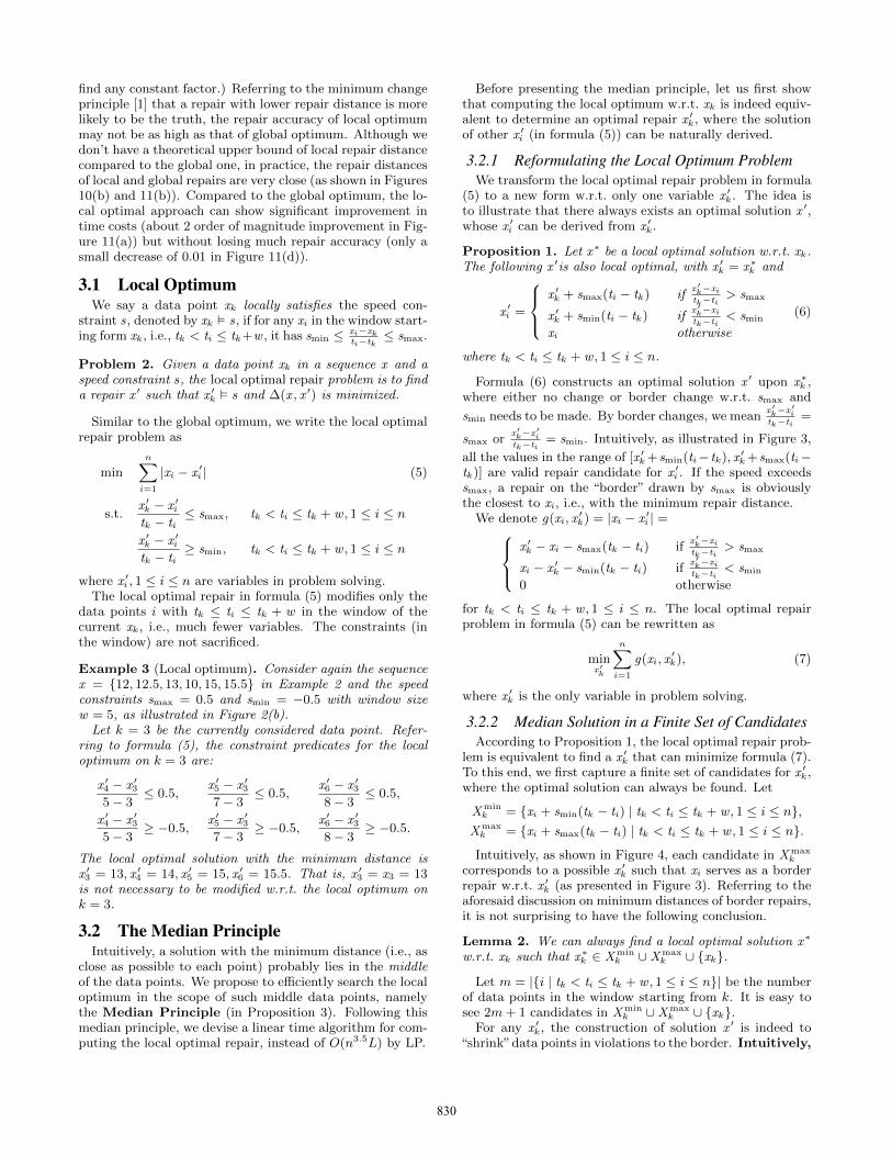
3.2.2 Median Solution in a Finite Set of CandidatesAccording to Proposition 1, the local optimal repair prob-

lem is equivalent to find a x ′k that can minimize formula (7).

To this end, we first capture a finite set of candidates for x ′k,

where the optimal solution can always be found. Let

Xmink = {xi + smin(tk − ti) | tk < ti ≤ tk + w , 1 ≤ i ≤ n},

Xmaxk = {xi + smax(tk − ti) | tk < ti ≤ tk + w , 1 ≤ i ≤ n}.

Intuitively, as shown in Figure 4, each candidate in Xmaxk

corresponds to a possible x ′k such that xi serves as a border

repair w.r.t. x ′k (as presented in Figure 3). Referring to the

aforesaid discussion on minimum distances of border repairs,it is not surprising to have the following conclusion.

Lemma 2. We can always find a local optimal solution x∗

w.r.t. xk such that x∗k ∈ Xmin

k ∪Xmaxk ∪ {xk}.

Let m = |{i | tk < ti ≤ tk + w , 1 ≤ i ≤ n}| be the numberof data points in the window starting from k. It is easy tosee 2m+ 1 candidates in Xmin

k ∪Xmaxk ∪ {xk}.

For any x ′k, the construction of solution x ′ is indeed to

“shrink”data points in violations to the border. Intuitively,

830

Figure 3: Build solution from x ′k Figure 4: Capture candidates for x ′

k Figure 5: Compute x ′k in integral repair

a candidate in the middle of all data points xi prob-ably has less shrink distances.

Let xmidk denote the median of all candidates,

xmidk = median(Xmin

k ∪Xmaxk ∪ {xk}). (8)

The following shows that the median xmidk is exactly the

optimal solution to the problem in formula (7), and can beused to build the local optimal solution by Proposition 1.

Proposition 3 (The Median Principle). A solution x ′ withx ′i determined by formula (6) and x ′

k = xmidk is local optimal.

Example 4 (Candidates and local optimum, Example 3continued). Consider data points 4, 5 and 6, in Figure 2(b),whose timestamps are within t3+w, w.r.t. the current k = 3.Each data point suggests two candidates w.r.t. smin and smax

for Xmin3 and Xmax

3 , respectively. For instance, x4 = 10contributes 10−0.5(5−3) = 9 in Xmax

3 and 10+0.5(5−3) =11 in Xmin

3 . Finally, the candidate sets are

Xmin3 ={11, 17, 18}, Xmax

3 ={9, 13, 13}.

According to formula (8), we have xmid3 = 13.

Referring to Proposition 3, by x ′3 = xmid

3 and formula (6),we build a solution x ′

3 = 13, x ′4 = 14, x ′

5 = 15, x ′6 = 15.5. It

is exactly the local optimal solution in Example 3.

3.3 Streaming ComputationThe integral cleaning algorithm is to iteratively determine

the local optimal x ′k, for k = 1, 2, . . . . Let us first assume

that data points come in-order, i.e., tj < ti for any j < i.(The handling of out-of-order arrival will be introduced inthe next section.)

3.3.1 Candidate RangeConsider xk, where x ′

1, . . . , x′k−1 have been determined in

the previous steps. Referring to the speed constraints, eachfixed x ′

j , tk − w ≤ tj < tk, 1 ≤ j < k, indicates a range ofcandidates for x ′

k, i.e., [x′j + smin(tk − tj), x

′j + smax(tk − tj)].

The following proposition states that considering the lastx ′k−1 is sufficient to determine the range of possible repairsfor x ′

k. The rationale is that for any 1 ≤ j < i < k, x ′i should

be in the range specified by x ′j as well. In other words, the

candidate range of x ′k specified by x ′

i is subsumed in therange by x ′

j .

Proposition 4. For any 1 ≤ j < i < k, tk − w ≤ tj <ti < tk, we have x ′

j + smin(tk − tj) ≤ x ′i + smin(tk − ti), and

x ′i + smax(tk − ti) ≤ x ′

j + smax(tk − tj).

For instance, as illustrated in Figure 5, the candidaterange of x ′

k specified by x ′k−2 subsumes that by x ′

k−1. Con-sequently, we can obtain a tight range of candidates for x ′

k

by x ′k−1, i.e., [x

mink , xmax

k ] as presented in Figure 5, where

xmink = x ′

k−1 + smin(tk − tk−1), (9)

xmaxk = x ′

k−1 + smax(tk − tk−1).

The repair problem thus becomes to finding the local op-timum x ′

k in the range of [xmink , xmax

k ].

3.3.2 Optimal Solution in Candidate RangeFormula (8) gives a repair candidate xmid

k suggested by xiafter xk (tk < ti), while formula (9) indicates a candidaterange [xmin

k , xmaxk ] specified by xk−1 before xk.

If the suggested local optimal solution xmidk in formula (8)

drops into the range of [xmink , xmax

k ] in formula (9), the opti-mal solution is directly obtained, i.e., x ′

k = xmidk . Otherwise,

we need to re-calculate the local optimum w.r.t. the range[xmin

k , xmaxk ].

Fortunately, we have the following monotonicity of thefunction in formula (7).

Proposition 5. For any u1, u2, v1, v2 ∈ Xmink ∪Xmax

k ∪{xk}such that u1 ≤ u2 ≤ xmid

k ≤ v1 ≤ v2, we have

n∑i=1

g(xi, u1) ≥n∑

i=1

g(xi, u2) ≥n∑

i=1

g(xi, xmidk ),

n∑i=1

g(xi, xmidk ) ≤

n∑i=1

g(xi, v1) ≤n∑

i=1

g(xi, v2).

That is, for any candidate u < xmaxk < xmid

k , it always has∑ni=1 g(xi, u) ≥

∑ni=1 g(xi, x

maxk ). xmax

k is thus the optimal

solution in the range of [xmink , xmax

k ]. Similar conclusion canalso be made for v > xmin

k > xmidk .

Consequently, according to Proposition 5, the local opti-mal solution is directed computed by

x ′k =

xmaxk if xmax

k < xmidk

xmink if xmin

k > xmidk

xmidk otherwise

(10)

Algorithm 1 presents the integral repair of a sequence xw.r.t. local optimum under the speed constraint s. For eachdata point k in the sequence, k = 1, 2, . . . , n, Lines 3 and 4computes the candidate range in formula (9). By consideringall the succeeding data points i in the window of k, Line10 calculates xmid

k in formula (8). Finally, x′k is obtained

following the computation in formula (10).It is easy to see that the number of distinct data points

in a window is at most w . The median in the window canbe trivially found in O(w), i.e., the average complexity ofquickselect [9]. Considering all the n data points in the se-quence, Algorithm 1 runs in O(nw) time. For a fixed w , it is

831

Algorithm 1: Local(x , s)

Data: an ordered sequence x and speed constraints sResult: a repair x ′ of x w.r.t. local optimum

1 for k ← 1 to n do2 Xmin

k ← ∅; Xmaxk ← ∅;

3 xmink ← x ′

k−1 + smin(tk − tk−1), or −∞ for k = 1;4 xmax

k ← x ′k−1 + smax(tk − tk−1), or +∞ for k = 1;

5 for i← k + 1 to n do // compute xmidk

6 if ti > tk + w then7 break;

8 Xmink ← Xmin

k ∪ {xi + smin(tk − ti)};9 Xmax

k ← Xmaxk ∪ {xi + smax(tk − ti)};

10 xmidk ← median(Xmin

k ∪Xmaxk ∪ {xk});

11 if xmaxk < xmid

k then // compute x ′k

12 x ′k ← xmax

k ;

13 else if xmink > xmid

k then14 x ′

k ← xmink ;

15 else16 x ′

k ← xmidk ;

17 return x ′

a linear time, constant space algorithm. In practice, to min-imize the changes, we may heuristically skip the repairingon those points xk that satisfy the speed constraints with itsneighbors, i.e., xmin

k ≤ xk ≤ xmaxk and xmin

k+1 ≤ xk+1 ≤ xmaxk+1 .

Example 5 (Example 4 continued). Consider the next datapoint k = 4 in the current sequence {12, 12.5, 13, 10, 15, 15.5},in Figure 2(b). According to formula (9), a candidate range[xmin

k , xmaxk ] = [12, 14] is given by x ′

3 = 13 (which is deter-mined in the previous step in Example 4).

Following the same line of Example 4, we compute Xmin4 =

{16, 17} and Xmax4 = {14, 14} by points 5 and 6 that are in

the window of point 4. It follows xmid4 = 14, which is in

the candidate range [12, 14]. According to formula (10), thelocal optimal repair on k = 4 is x ′

4 = 14.The integral repair moves on to the next k = 5 and ter-

minates when reaching the end of the sequence. A repairedsequence {12, 12.5, 13, 14, 15, 15.5} is finally returned.

4. OUT-OF-ORDER CLEANINGWhen a delayed data point comes, the straightforward ap-

proach is to insert the data point into the right position ofthe sequence according to timestamps, and recompute allthe results for data points near (and after) the inserted po-sition. However, complete re-computation is not necessary.Instead, we can efficiently update the repairs over the previ-ously computed results. To further reduce the computation,we propose a heuristic strategy that updates the results onlywhen the previous results are known to be invalid for sure.

4.1 Updating Local OptimumConsider an out-of-order arrival xk, tk < tk−1. We reorder

the sequence by timestamps, i.e., removing xk and insertingit as a new x` where x` = xk, t`−1 < t` < t`+1, ` < k.

The updates introduced by x` include two aspects: (1) forxj , j < `, where x` suggests candidates for determine xmid

j ;

and (2) for xi, i > `, whose candidate range [xmini , xmax

i ] isinfluenced (directly or indirectly) by x ′

`.

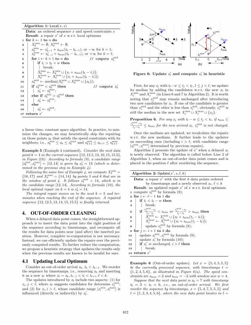
Figure 6: Update x ′` and compute x ′

` in heuristic

First, for any xj with t`−w ≤ tj < t`, 1 ≤ j < `, we updateits median by adding the candidates w.r.t. the new x` inXmin

j and Xmaxj (in Lines 6 and 7 in Algorithm 2). It is worth

noting that xmidj may remain unchanged after introducing

two new candidates by x`. If one of the candidate is greaterthan xmid

j and the other is less than xmidj , obviously, xmid

j is

still the median in the new set Xminj ∪Xmax

j ∪ {xj}.

Proposition 6. For any xj with t` −w ≤ tj < t`, if smin ≤xmidj −x`tj−t`

≤ smax for the new arrived x`, xmidj is not changed.

Once the medians are updated, we recalculate the repairsw.r.t. the new medians. It further leads to the updateson succeeding ones (including i > `, with candidate range[xmin

i , xmaxi ] determined by previous repairs).

Algorithm 2 presents the update of x ′ when a delayed x`is newly observed. The algorithm is called before Line 2 ofAlgorithm 1, when an out-of-order data point comes and isplaced in the position ` after reordering the sequence.

Algorithm 2: Update(x ′, s, `, k)

Data: a repair x ′ with the first k data points orderedby timestamps and a newly observed x`, ` < k

Result: an updated repair x ′ of x w.r.t. local optimum1 compute xmid

` by formula (8);2 for i← `− 1 to 1 do3 if ti < t` − w then4 break;

5 ifxmidj −x`tj−t`

< smin orxmidj −x`tj−t`

> smax then

6 Xminj ← Xmin

j ∪ {x` + smin(tj − t`)};7 Xmax

j ← Xmaxj ∪ {x` + smax(tj − t`)};

8 update xmidj by formula (8);

9 for j ← i+ 1 to k do10 update xmin

i , xmaxi by formula (9);

11 update x ′i by formula (10);

12 if x ′i is unchanged, i > ` then

13 break;

14 return x ′

Example 6 (Out-of-order update). Let x = {5, 4, 5, 5, 5}be the currently processed sequence, with timestamps t ={1, 2, 4, 5, 6}, as illustrated in Figure 6(a). The speed con-straints are smax = 2 and smin = −2 with window size w = 4.

Suppose that the next data point is x6 = 7 with timestampt6 = 3 < t5 = 6, i.e., an out-of-order arrival. We firstreorder the sequence by timestamps, x = {5, 4, 7, 5, 5, 5} andt = {1, 2, 3, 4, 5, 6}, where the new data point locates in ` =

832

3. Referring to the window size w = 4, data points 1 and 2are influenced by the new point.

For x1, suppose that xmid1 = 5 before the new point ` is

inserted. We computexmid1 −x`t1−t`

= 5−71−3

= 1, which is in the

range [smin, smax]. According to Proposition 6, xmid1 = 5 will

not be changed after inserting `. For x2, we have xmid2 = 4

before inserting ` and 4−72−3

= 3 > smax. That is, xmid2 should

be updated after inserting `, having xmid2 = 5. And xmid

3 = 7for ` = 3 can also be computed by formula (8). Since xmid

2

is updated and xmid3 is newly introduced, the repair should be

refreshed following formula (10), i.e., x ′ = {5, 5, 7, 5, 5, 5}.

4.2 HeuristicAlthough exact result w.r.t. local optimum is guaranteed,

the update (possibly on all the data points near and afterx`) is costly. If a data point is delayed at the very beginningof the sequence, almost the entire sequence may be updated.

Heuristically, we could choose to update only when theexisting repairs are found to be invalid for sure. That is,after inserting the data point on position `, the existing x ′

violates speed constraints (no matter what the value x ′` is).

Such invalid scenario occurs, because of the disagreementon the possible values for x ′

`. The existing repair x ′`−1 speci-

fies a range of possible repairs for x ′`, as presented in formula

(9). Symmetrically, x ′`+1 as an existing repair also indicates

another range for x ′`. Contradiction between two ranges may

occur (if x ′`+1 is not in the window of x ′

`−1).We capture the minimum and maximum candidates for x ′

`

that are specified by x ′`−1 and x ′

`+1 together,

xmin` = max(x ′

`−1 + smin(t` − t`−1), x′`+1 + smax(t` − t`+1)),

xmax` = min(x ′

`−1 + smax(t` − t`−1), x′`+1 + smin(t` − t`+1)),

(11)

where t`+1 − t`−1 ≤ 2 · w . Here, xmin` takes the maximum

of bounds (in formula (9)) determined by ` − 1 and ` + 1,as illustrated in Figure 6(b), and similarly xmax

` takes thelower one of the bounds given by ` − 1 and ` + 1. In otherwords, a x ′

` within the range [x ′`−1, x

′`+1] will satisfy the speed

constraints w.r.t. both `− 1 and `+ 1.Obviously, if xmin

` > xmax` , contradiction occurs. That is,

the current repair x ′ is invalid, and the update by Algorithm2 should be performed.

On the other hand, if valid candidates exist, i.e., xmin` ≤

xmax` , we can heuristically select a repair x ′

` in [xmin` , xmax

` ]without updating the others. As shown in Lines 3 and 4in Algorithm 3, x` is taken as xmid

` in heuristic. Accordingto formula (10), x ′

` leaves unchanged if x` is in [xmin` , xmax

` ].Otherwise, the border xmin

` or xmax` , which is closer to x`, is

assigned as the repair x ′`.

A natural concern is how often the full Update in Line 7in Algorithm 3 occurs. We show in the following conclusionthat Update would never be performed if the time intervalt`+1 − t`−1 is within w .

Proposition 7. For any xmin` > xmax

` computed by formula(11), it always has w < t`+1 − t`−1 ≤ 2 · w.

In other words, the Update may occur only when t`−1 andt`+1 are far away (> w). In practice, such large “breaks”appear rarely especially in continuous monitoring streams.By greatly avoiding Update, the Heuristic approach can sig-nificantly reduce the repair time costs (in the experiments).

Algorithm 3: Heuristic(x ′, s, `, k)

Data: a repair x ′ with the first k dat points ordered bytimestamps and a newly observed x`, ` < k, andspeed constraints s

Result: an updated repair x ′ of x w.r.t. local optimum1 compute xmin

` , xmax` by formula (11);

2 if xmin` ≤ xmax

` then3 xmid

` ← x`;4 compute x ′

` by formula (10);5 return x ′

6 else7 return Update(x ′, s, `, k)

Example 7 (Heuristic, Example 6 continued). Consideragain the reordered sequence, x = {5, 4, 7, 5, 5, 5} with times-tamps t = {1, 2, 3, 4, 5, 6}, where ` = 3 is the newly inserteddata point, as illustrated in Figure 6(a).

Referring to formula (9), data point `−1 gives a candidaterange [2, 6] for x ′

` w.r.t. the speed constraints smax = 2 andsmin = −2. Symmetrically, another candidate range [3, 7]for x ′

` is also determined by `+1. By taking the intersectionof two candidate ranges, we have [xmin

` , xmax` ] = [3, 6] as

defined in formula (11). Since xmin` ≤ xmax

` , we heuristicallydetermine the repair x ′

3 = 6 without update the other repairresults, having x ′ = {5, 4, 6, 5, 5, 5}.

5. ADAPTIVE WINDOWSThe trade-off in setting window size w for speed con-

straints is: small windows fail to capture the minimum re-pair (e.g., if w=1 in Figure 2(b) of Example 2), while largewindows obviously increase the computation overhead (asmore constrained data pairs need to be specified in formulas(3) for global optimum or (5) for local optimum). It is non-trivial to predefine an appropriate window size. Even worse,the arrival rate (the number of data points in a period) mayvary. Rather than a fixed window size, we propose to auto-matically determine the adaptive window size w online.

To tackle the aforesaid trade-off in choosing window sizes,we introduce a statistical sampling-based method. The ideais to model data points as random samples of approachingthe speed constraints. The adaption of windows, extendingor shrinking, is thus performed based on the closeness to theextreme speeds (smax or smin) of the samples, grounded instatistical sampling theory.

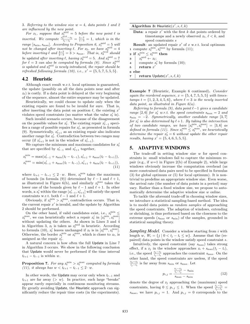
Sampling Model. Consider a window starting from i withlength w , Wi = {j | 0 < tj − ti ≤ w}. Assume that the (re-paired) data points in the window satisfy speed constraint s.

Intuitively, the speed constraint (say smax) takes strongeffect, if a xj in the window approaches xi + smax(tj − ti),

i.e., the speedxj−xitj−ti

approaches the constraint smax. On the

other hand, the speed constraints are useless, if the speedxj−xitj−ti

is far away from smin or smax. Let

pi,j =

xi−xjti−tj

− smin

smax − smin(12)

denote the degree of xj approaching the (maximum) speed

constraints, having 0 ≤ pi,j ≤ 1. When the speedxj−xitj−ti

=

smax, we have pi,j = 1. And pi,j = 0 corresponds to the

833

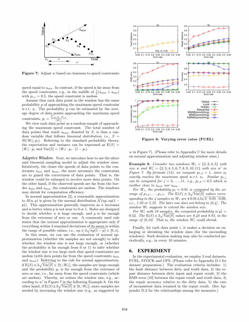
Figure 7: Adjust w based on closeness to speed constraints

speed equal to smin. In contrast, if the speed is far away fromthe speed constraints, e.g., in the middle of 1

2(smax + smin)

with pi,j = 0.5, the speed constraint is useless.Assume that each data point in the window has the same

probability p of approaching the maximum speed constraintw.r.t. xi. The probability p can be estimated by the aver-age degree of data points approaching the maximum speed

constraints, pi =∑

j∈Wipi,j

|Wi|.

We view each data point as a random sample of approach-ing the maximum speed constraint. The total number ofdata points that reach smax, denoted by S , is thus a ran-dom variable that follows binomial distribution, i.e., S ∼B(|Wi|, pi). Referring to the standard probability theory,the expectation and variance can be expressed as E(S) =|Wi| · pi and Var[S ] = |Wi| · pi · (1− pi).

Adaptive Window. Next, we introduce how to use the afore-said binomial sampling model to adjust the window sizes.Intuitively, the closer the speeds of data points to the con-straints smin and smax, the more necessary the constraintsare to guard the correctness of data points. That is, thewindow could be enlarged to involve more data points. Onthe other hand, if the observed speeds are far from the bor-der smin and smax, the constraints are useless. The windowsmay shrink for computation efficiency.

In normal approximation [2], a reasonable approximationto B(n, p) is given by the normal distribution N (np, np(1−p)). This approximation generally improves as n increasesand is better when p is not near to 0 or 1. Rules are designedto decide whether n is large enough, and p is far enoughfrom the extremes of zero or one. A commonly used rulestates that the normal approximation is appropriate only ifeverything within 3 standard deviations of its mean is withinthe range of possible values, i.e., np± 3

√np(1− p) ∈ [0, n].

In this sense, we can use the evaluation of normal ap-proximation (whether the samples are not enough) to inferwhether the window size is not large enough, or (whetherthe probability is far enough from 0 or 1) to infer whetherthe window size is too large such that speed constraints areuseless (with data points far from the speed constraints smin

and smax). Referring to the rule for normal approximation,

if E(S)±3√

Var[S ] ∈ [0, |Wi|], the samples are large enoughand the probability pi is far enough from the extremes ofzero or one, i.e., far away from the speed constraints (whichare useless). Thereby, we reduce the window size, e.g., ac-cording to w ′ in Figure 7 in the following Example 8. On theother hand, if E(S)±3

√Var[S ] 6∈ [0, |Wi|], more samples are

needed by increasing the window size (e.g., as suggested by

0

0.1

0.2

0.3

0.4

0.5

0.6

0.05 0.1 0.15 0.2 0.25 0.3 0.35 0.4 0.45

Fault d

ista

nce

Error rate

(a)

dirty vs. truth 0

0.1

0.2

0.3

0.4

0.5

0.6

0.05 0.1 0.15 0.2 0.25 0.3 0.35 0.4 0.45

Repair d

ista

nce

Error rate

(b)

0

0.1

0.2

0.3

0.4

0.5

0.6

0.05 0.1 0.15 0.2 0.25 0.3 0.35 0.4 0.45

RM

S e

rror

Error rate

(c)

0

0.2

0.4

0.6

0.8

1

0.05 0.1 0.15 0.2 0.25 0.3 0.35 0.4 0.45

Accura

cy

Error rate

(d)

0

0.2

0.4

0.6

0.8

1

0.05 0.1 0.15 0.2 0.25 0.3 0.35 0.4 0.45In

consis

tency r

ate

Error rate

(e)GlobalLocal

HolisticSequential

SWAB(smoothing)WMA(smoothing)

EWMA(smoothing)

Figure 8: Varying error rates (FUEL)

w in Figure 7). (Please refer to Appendix C for more detailson normal approximation and adjusting window sizes.)

Example 8. Consider two windows W1 = {2, 3, 4, 5} withsize w and W ′

1 = {2, 3, 4, 5, 6, 7, 8, 9, 10, 11} with size w ′ inFigure 7. By formula (12), we compute p1,2 = 1, since x2exactly reaches the maximum speed w.r.t. x1. Similar p1,jcan be computed for j = 3, . . . , 11, e.g., p1,8 = 0.5 which isneither close to smax nor smin.For W1, the probability p1 = 0.91 is computed by the av-

erage of p1,2, . . . , p1,5. The E(S) ± 3√

Var[S ] values corre-

sponding to the 4 samples in W1 are 4·0.91±3√4 · 0.91 · 0.09,

i.e., 1.92 or 5.35. The later one does not belong to [0,4]. Thewindow W1 suggests to extend the window size.

For W ′1 with 10 samples, the computed probability is p′1 =

0.52. The E(S)±3√

Var[S ] values are 0.46 and 9.93, in therange of [0,10]. That is, the window W ′

1 could shrink.

Finally, for each data point i, it makes a decision on en-larging or shrinking the window sizes (for the succeedingwindows). Such decision making may also be conducted pe-riodically, e.g., in every 10 minutes.

6. EXPERIMENTIn the experimental evaluation, we employ 3 real datasets,

FUEL, STOCK and GPS. (Please refer to Appendix D.1 fordataset preparation.) The evaluation criteria includes: 1)the fault distance between dirty and truth data, 2) the re-pair distance between dirty input and repair result, 3) theRMS error [10] between the repair result and truth data, 4)the repair accuracy relative to the dirty data, 5) the rateof inconsistent data retained in the repair result. (See Ap-pendix D.2 for the relationships among the measures.)

834

0

5

10

15

20

25

0.05 0.1 0.15 0.2 0.25 0.3 0.35 0.4 0.45

Fault d

ista

nce

Error rate

(a)

dirty vs. truth 0

5

10

15

20

25

0.05 0.1 0.15 0.2 0.25 0.3 0.35 0.4 0.45

Repair d

ista

nce

Error rate

(b)

0

5

10

15

20

25

0.05 0.1 0.15 0.2 0.25 0.3 0.35 0.4 0.45

RM

S e

rror

Error rate

(c)

0

0.2

0.4

0.6

0.8

1

0.05 0.1 0.15 0.2 0.25 0.3 0.35 0.4 0.45

Accura

cy

Error rate

(d)

0

0.2

0.4

0.6

0.8

1

0.05 0.1 0.15 0.2 0.25 0.3 0.35 0.4 0.45

Inconsis

tency r

ate

Error rate

(e)GlobalLocal

HolisticSequential

SWAB(smoothing)WMA(smoothing)

EWMA(smoothing)

Figure 9: Varying error rates (STOCK)

Table 1: GPS data with manually labeled ground truth

Method Repairdistance

RMSerror

Accuracy Inconsistency

Global 0.1198 0.0658 0.6881 –

Local 0.1311 0.0682 0.6886 –

Holistic 0.1197 0.0653 0.6842 0.0403

Sequential 0.9589 0.9646 0.0001 0.1285

SWAB 0.6368 0.6372 0.0649 0.0639

WMA 1.5700 1.5627 0.0184 0.1492

EWMA 1.7054 1.6993 0.0166 0.0556

6.1 Comparison with Existing ApproachesIn the first experiment, we compare our proposed SCREEN

with Global and Local optimum to the following approachesin two categories: 1) smoothing-based, SWAB [13], WMAand EWMA [7], and 2) constraint-based, Holistic repair [4]and repair with Sequential Dependency [8].

Figures 8 and 9 consider various error rates (denoting theamount of injected errors) with data sizes (the number ofdata points/the length of the sequence) 3k and 2k, in FUELand STOCK, respectively. Figures 10 and 11 study the scal-ability by varying data sizes (with error rate 0.3 and 0.2).The full results of all compared methods are in Figures 18and 19. Table 1 presents the results over the GPS datasetwith manually labeled ground truth.

First, it is not surprising that RMS error of all the smooth-ing methods is high, while their accuracy is lower, comparedwith our proposed Global or Local (e.g., in Table 1). As illus-trated in Figure 8(b), the repair distances of SWAB, WMA

0.01

0.1

1

10

100

1000

10000

6k 12k 18k 24k 30k

Tim

e c

ost (s

)

Data size

(a)

GlobalLocal

0

5

10

15

20

25

30

35

40

45

6k 12k 18k 24k 30k

Repair d

ista

nce

Data size

(b)

GlobalLocal

0

0.02

0.04

0.06

0.08

0.1

0.12

6k 12k 18k 24k 30k

RM

S e

rror

Data size

(c)

GlobalLocal

0

0.2

0.4

0.6

0.8

1

6k 12k 18k 24k 30k

Accura

cy

Data size

(d)

GlobalLocal

Figure 10: Global vs. Local (FUEL)

0.001

0.01

0.1

1

10

100

2k 4k 6k 8k 10k

Tim

e c

ost (s

)

Data size

(a)

GlobalLocal

0

5

10

15

20

2k 4k 6k 8k 10k

Repair d

ista

nce

Data size

(b)

GlobalLocal

0

1

2

3

4

5

2k 4k 6k 8k 10k

RM

S e

rror

Data size

(c)

GlobalLocal

0

0.2

0.4

0.6

0.8

1

2k 4k 6k 8k 10k

Accura

cy

Data size

(d)

GlobalLocal

Figure 11: Global vs. Local (STOCK)

and EWMA smoothing are very similar. These smoothingmethods show similar RMS error and accuracy as well inFigures 8(c)(d). It is notable that the inconsistency ratesof smoothing are very high in Figure 8(e). That is, a largenumber of data points are still in violation w.r.t. speed con-straints. The corresponding accuracy of smoothing is thussignificantly lower than our proposal in Figure 8(d).

Holistic repair, the approximation of our Global as in-troduced in Appendix B, show similar accuracy as Global.However, its time cost is close to the exact approach Globalas well. Even worse, as shown in Figures 8(e), the inconsis-tency rate of Holistic is high. An inconsistency rate 0.4 de-notes that about 40% data points are still involved in viola-tion to speed constraints, after Holistic repair. For STOCKwith window size w = 1, there are fewer constraint pred-icates declared between data points. Therefore, inconsis-tencies remained after Holistic repair are fewer as well, i.e.,lower inconsistency rate in Figures 9(e).

Sequential dependencies (SDs) consider the constraints onvalue difference (e.g., ≤ 5) of two consecutive data points.When the time interval of any two consecutive data pointsis the same, for instance, in every trading day or in every 5minutes, SDs denote exactly the speed constraints. There-

835

0.1

1

10

100

0.2 0.4 0.6 0.8 0.1

Tim

e c

ost (s

)

Delay rate

(a)

UpdateHeuristic

0

0.2

0.4

0.6

0.8

1

0.2 0.4 0.6 0.8 0.1

Accura

cy

Delay rate

(b)

UpdateHeuristic

0.1

1

500 1000 2000 3000 5000

Tim

e c

ost (s

)

Delay time

(c)

UpdateHeuristic

0

0.2

0.4

0.6

0.8

1

500 1000 2000 3000 5000

Accura

cy

Delay time

(d)

UpdateHeuristic

Figure 12: Evaluation on out-of-order (FUEL)

0.01

0.1

1

0.2 0.4 0.6 0.8 0.1

Tim

e c

ost (s

)

Delay rate

(a)

UpdateHeuristic

0

0.2

0.4

0.6

0.8

1

0.2 0.4 0.6 0.8 0.1

Accura

cy

Delay rate

(b)

UpdateHeuristic

0.01

0.1

1

100 300 500 1000 2000

Tim

e c

ost (s

)

Delay time

(c)

UpdateHeuristic

0

0.2

0.4

0.6

0.8

1

100 300 500 1000 2000

Accura

cy

Delay time

(d)

UpdateHeuristic

Figure 13: Evaluation on out-of-order (STOCK)

fore, in STOCK, the accuracy of Sequential is relativelyhigh, while its RMS error is low (compared with SWAB).However, if the data point arrival is dynamic without a fixedtime interval, such as FUEL, SDs can no longer denote thespeed semantics. Consequently, the performance of Sequen-tial is low in Figures 8(c)(d), even worse than SWAB.

The repair distance of Global is always lower than thatof Local, in Figures 10(b) and 11(b). The correspondingRMS error of Global is lower in Figures 10(c) and 11(c) andthe repair accuracy of Global is higher in Figures 10(d) and11(d). Nevertheless, the Local method have very similarrepair distance and accuracy to Global, especially comparedwith the other baseline approaches in Figures 18 and 19. Theresults verify our analysis (e.g., ∆(x , xlocal) ≥ ∆(x , xglobal)at the beginning of Section 3), and demonstrate the timeand accuracy performance of Local optimum compared toGlobal in practice.

6.2 Evaluation over Streaming DataNext, we evaluate the online cleaning over streaming data.

Since none of the existing methods support out-of-order ar-rivals, we mainly compare the proposed Update technique inAlgorithm 2 and Heuristic in Algorithm 3 for handling de-

0.001

0.01

0.1

1

10

100

1000

10 50 100500

10001500

30005000

10000

INF

Tim

e c

ost (s

)

Window size

(a)

GlobalLocal

SWABWMA

EWMA

0

0.2

0.4

0.6

0.8

1

10 50 100500

10001500

30005000

10000

INF

Accura

cy

Window size

(b)

LocalSWABWMA

EWMAGlobal

Figure 14: Evaluation on various window sizes

0.0001

0.001

0.01

0.1

0.05 0.1 0.15 0.2 0.25 0.3 0.35 0.4 0.45

Tim

e c

ost (s

)

Error rate

(a)

T=AdaptiveT=10

T=100T=1000T=1500

0

0.2

0.4

0.6

0.8

1

0.05 0.1 0.15 0.2 0.25 0.3 0.35 0.4 0.45

Accura

cy

Error rate

(b)

T=AdaptiveT=10

T=100T=1000T=1500

10000

100000

1e+06

1e+07

1e+08

0.05 0.1 0.15 0.2 0.25 0.3 0.35 0.4 0.45

Thro

ughoutp

ut

Error rate

(c)

T=AdaptiveT=10

T=100T=1000T=1500

0

200

400

600

800

1000

0.05 0.1 0.15 0.2 0.25 0.3 0.35 0.4 0.45

Adaptive w

indow

siz

e

Error rate

(d)

Adaptivew=10

w=100w=1000w=1500

Figure 15: Evaluation on adaptive window sizes

layed data points. Figures 12 and 13 report the out-of-orderevaluation, by varying delay rate (e.g., 0.1 denotes that 10%of data points are delayed in arrival) and delay time (refer-ring to the average distance between the actual timestampand the arrival time). Settings of delay time for Figures12(a)(b) and 13(a)(b) are 5000 and 1000, respectively, andthe delay rate in Figures 12(c)(d) and 13(c)(d) is 0.05.

Generally, the larger the delay rate or delay time is, thehigher the time costs are. For Heuristic, since the full updateoccurs only when the previously repaired results are foundto be wrong for sure, its time cost is significantly lower. Asshown in Figures 12 and 13, Heuristic method has compa-rable accuracy with Update, while the former one can show1-2 orders of magnitude improvement in time costs.

6.3 Evaluation on Adaptive WindowsThis experiment evaluates the cleaning performance under

various window sizes of speed constraints. Since the windowsize is fixed to 1 for STOCK, we focus on the FUEL dataset(with data size 3k, and error rate 0.05 for Figure 14).

As shown in Figure 14, the Local method requires a bitlarger window size (e.g., 100) to achieve the same accuracyof Global (at 50). For a window larger than 500, both Globaland Local have considerably high accuracy. The time cost ofan infinite window (INF, throughout the lifetime of the datastream) is extremely high, while a smaller window size (e.g.,500) that has much lower time cost can achieve an accuracyas high as INF. The results verify that, in a real setting, it isnot necessary to consider extremely large windows, since asmall window size is sufficient to achieve the same accuracywith significantly lower time cost. On the other hand, if thewindow size is too small, e.g., w = 10 in Figure 14, many

836

0

0.05

0.1

0.15

0.2

(-200,-180]

(-160,-140]

(-120, -100]

(-80, -60]

(-40, -20]

Dis

trib

ution

Speed (L/h)

(a) FUEL

0

0.05

0.1

0.15

0.2

0.25

(1,2]

(3,4]

(5,6]

(7,8]

(9,10]

Dis

trib

ution

Speed (m/s)

(b) GPS

Figure 16: Statistical distribution on speeds

0

0.2

0.4

0.6

0.8

1

-1.2-2 -4 -20

-40-80

-100-120

-160

Accura

cy

Smin (L/h)

(a) FUEL

0

0.2

0.4

0.6

0.8

1

4 5 6 6.5 7 8 9 10 21

Accura

cy

Smax (m/s)

(b) GPS

0

0.2

0.4

0.6

0.8

1

0.001

0.010.1

0.30.7

1 3 8 15 40

Accura

cy

Smax (-Smin, $/d)

(c) STOCKLocal

SWAB(smoothing)WMA(smoothing)

EWMA(smoothing)

Figure 17: Evaluation on various speed constraints

data points will be out of control by the speed constraints,and fewer repairs are performed. The repair accuracy is thuslower (even lower than the smoothing baselines).

Nevertheless, as illustrated in Figure 15, our adaptive win-dow technique can determine an appropriate window size(around 700), which shows relatively low time cost and highthroughput without losing much accuracy. These resultsverify our trade-off analysis between cleaning accuracy andefficiency in Section 5. In other words, our proposed adap-tive windows can balance the effectiveness and efficiency.

6.4 Capturing Speed ConstraintsWe note that in most scenarios, the speed constraint is

natural, e.g., the fuel consumption of a crane should not benegative (smax = 0 for FUEL), while some others could bederived. According to our consultation with experts of theequipment, the fuel consumption does not exceed 40 litersper hour (smin = −40). For STOCK, the speed constraintsare naturally derived by the business semantics. The pricelimit in the market declares that the increase or decrease ofdaily price should not exceed l · r where l is the price of thelast trading day and r = 10% is a percentage. We considerthe highest price h = 60 in the dataset, having l ≤ h for anyday in the period. The maximum speed smax (with w = 1)in the period is thus h ·r = 6, while smin = −h ·r = −6. TheGPS dataset is collected by a person carrying a smartphoneand walking around at campus. We require 7 meters persecond as the maximum walking speed of the person.

Nevertheless, for a particular domain where speed knowl-edge is not available, the speed constraints can be extractedfrom data. We consider the statistical distribution of speedsby sampling data pairs over FUEL and GPS in Figure 16.

0.001

0.01

0.1

1

10

100

1000

10000

6k 12k 18k 24k 30k

Tim

e c

ost (s

)

Data size

(a)

0

0.1

0.2

0.3

0.4

0.5

0.6

0.7

0.8

6k 12k 18k 24k 30k

Repair d

ista

nce

Data size

(b)

0

0.1

0.2

0.3

0.4

0.5

0.6

0.7

0.8

6k 12k 18k 24k 30k

RM

S e

rror

Data size

(c)

0

0.2

0.4

0.6

0.8

1

6k 12k 18k 24k 30k

Accura

cy

Data size

(d)

GlobalLocal

HolisticSequential

SWAB(smoothing)WMA(smoothing)

EWMA(smoothing)

Figure 18: Scalability (FUEL)

As mentioned, the FUEL meter change is non-increasing(smax = 0) during consumption, while the walking speed forGPS is non-negative (smin = 0). Thereby, we mainly ob-serve the speeds for determining smin for FUEL and smax

for GPS. Referring to statistics, it is to determine a confi-dence interval that acts as a good estimate of the unknownpopulation parameter smin (smax). In applied practice, con-fidence intervals are typically stated at the 95% confidencelevel [11]. In other words, 95% of the speeds are regarded asaccurate (within smin or smax). It suggests smax = 7 for GPSand smin = −80 for FUEL (although the expert’s suggestionis -40 in the experiments). As illustrated in Figure 17, givensuch speed constraints (either -80 or -40 for FUEL), the ac-curacies are much higher than the smoothing baselines.

Generally, if the speed constraints are set too loose, e.g.,smin = −160 in Figure 17(a) or smax = 40 in Figure 17(c),almost everything will pass the examination of speed con-straints without repairing and thus the repair accuracy (ofLocal) is low. On the other hand, if the speed constraintsare too tight, say smax = 0.001 in Figure 17(c), most valueswould be regarded as violations to such tight constraints.With over-repairing, the corresponding repair accuracy islow too. Nevertheless, the accuracy of the constraint-basedmethod (Local) is higher than that of the constraint-obliviousbaselines, in a wide range of speed constraints, e.g., eitherthe expert suggested -40 or the aforesaid statistical sugges-tion -80 in Figure 17(a). For GPS data in Figure 17(b), thereis also a wide range, from 6 to 21, where the constraint-awareLocal clearly outperforms the constraint-oblivious baselines.Indeed, in common sense, it is irrational for a person walkingwith a speed greater than 21 meters per second.

6.5 Summary of ExperimentsWe summarize the experimental results as follows: 1) The

accuracy is significantly improved by our proposal (Globaland Local) compared to the existing SWAB, WMA andEWMA smoothing; 2) Without considering the precise speedconstraints, the existing SD-based repair has much lower ac-

837

0.001

0.01

0.1

1

10

100

2k 4k 6k 8k 10k

Tim

e c

ost (s

)

Data size

(a)

0

5

10

15

20

2k 4k 6k 8k 10k

Repair d

ista

nce

Data size

(b)

0

5

10

15

20

2k 4k 6k 8k 10k

RM

S e

rror

Data size

(c)

0

0.2

0.4

0.6

0.8

1

2k 4k 6k 8k 10k

Accura

cy

Data size

(d)

GlobalLocal

HolisticSequential

SWAB(smoothing)WMA(smoothing)

EWMA(smoothing)

Figure 19: Scalability (STOCK)

curacy than our Global and Local; 3) The proposed Localapproach with online cleaning supports shows orders of mag-nitude improvement in time costs compared to the Holisticmethod; 4) The heuristic update strategy significantly re-duces the time costs in handling out-of-order arrival; 5) Theadaptive window technique can automatically suggests anappropriate window size (around 700), which shows rela-tively low time costs without losing much accuracy.

7. RELATED WORK

Smoothing-based Data Cleaning. The SWAB smoothing[13] is a linear interpolation/regression-based, online smooth-ing method of stream data. With a sliding window, SWABuses linear interpolation or linear regression to find the ap-proximating line of a time series. Besides, the moving av-erage [3] is also commonly used to smooth time series dataand make forecasts. A simple moving average (SMA) is theunweighted mean of the last k data. This average is used forforecasting the next value of the time series. Whereas in thesimple moving average the past observations are weightedequally, a weighted moving average (WMA) multiplies fac-tors to give different weights to data at different positions inthe sample window, e.g., using the inverse value of time in-terval as the weight. Moreover, the exponentially weightedmoving average (EWMA) [7] assigns exponentially decreas-ing weights over time. It is obvious to see that all thesesmoothing methods will modify a large number of data points.Therefore, as the example illustrated in Figure 1, the majorissue of smoothing is the serious damage of the originallycorrect data points. One of our major contributions in thispaper is the employment of speed constraints to supervisethe more accurate cleaning. Following the minimum changeprinciple in constraint-based repairing, the original precisevalues are maximally preserved. Consequently, the accu-racy of our proposed method is much higher than that ofsmoothing, as observed in our experimental evaluation.

Constraint-based Data Repairing. To the best knowl-edge of our knowledge, Holistic cleaning [4] is the only ex-isting constraint-based technique that can support speedconstraints (expressed by denial constraints). Since the ap-proach is proposed for repairing the general (tableau) data,it cannot support the online/integral cleaning over slidingwindows in streaming data. In this sense, one of our contri-butions in this study is the SCREEN with local optimum,which supports not only online cleaning but also out-of-orderdata arrival. Consequently, as illustrated in the experiments,our proposal can show up to 4 orders of magnitude improve-ment in time costs compared with Holistic cleaning.

Moreover, Sequential Dependency (SD) [8] cannot expressprecisely the speed constraints. SDs concern the differenceof two consecutive data points in a sequence. As discussed,data streams often deliver data points in various time inter-vals. Given different timestamp distances, the value differ-ence of two consecutive points does not exactly denote thespeed semantics. Owing to such imprecise constraint knowl-edge, as presented in the experiments, the accuracy of SD(Sequential) based repair could be much lower compared toour speed constraint-based proposal. Our another contribu-tion is the employment of the more accurate speed ratherthan the simple value distance in repairing streaming data.

Besides our studied speed constraints, Fischer et al. [5]propose a nice notation, Stream Schema, for representingstructural and semantic constraints on data streams. TheStream Schema concerns general constraints with varioussemantics such as orderings between attribute values, whileour study focuses only on the specific speed constraints overnumeric values. As a promising future direction, it is inter-esting to extend the stream data cleaning w.r.t. the moregeneral Stream Schema constraints.

8. CONCLUSIONSIn this study, we first indicate the inappropriateness of the

smoothing-based stream data cleaning. It could not repairthe dirty data such as large spikes, and even worse may se-riously damage the originally accurate values. Following thesame line of employing integrity constraints for relationaldata cleaning, in this paper, we propose SCREEN, the firstconstraint-based stream data cleaning approach. The re-pairing of imprecise data is guided by the innovative con-straints on speed. The speed constraint semantics could beeasily captured, such as daily price limit in financial markets,or fuel consumption limit of devices. With speed constraints,SCREEN supports online streaming cleaning in linear time,out-of-order arrival of data points, and high throughput viaadaptive window sizes. In particular, the novelMedian Prin-ciple can fast identify the local optimum, following the in-tuition that a solution with the minimum distance (i.e., asclose as possible to each point) probably lies in the middle ofthe data points. Experiments on real datasets demonstratethat our SCREEN can show significantly higher repair accu-racy than the smoothing-based approach, and up to 4 ordersof magnitude improvement in time performance comparedto the state-of-the-art data cleaning methods.

AcknowledgementThis work is supported in part by China NSFC under Grants61325008, 61202008 and 61370055; US NSF through grantsCNS-1115234, and OISE-1129076.

838

9. REFERENCES

[1] P. Bohannon, M. Flaster, W. Fan, and R. Rastogi. Acost-based model and effective heuristic for repairingconstraints by value modification. In SIGMODConference, pages 143–154, 2005.

[2] G. E. P. Box. Statistics for experimenters: anintroduction to design, data analysis, and modelbuilding. 1978.

[3] D. R. Brillinger. Time series: data analysis andtheory, volume 36. Siam, 2001.

[4] X. Chu, I. F. Ilyas, and P. Papotti. Holistic datacleaning: Putting violations into context. In ICDE,pages 458–469, 2013.

[5] P. M. Fischer, K. S. Esmaili, and R. J. Miller. Streamschema: providing and exploiting static metadata fordata stream processing. In EDBT, pages 207–218,2010.

[6] Full Version.http://ise.thss.tsinghua.edu.cn/sxsong/doc/screen.pdf.

[7] E. S. Gardner Jr. Exponential smoothing: The stateof the art–part ii. International Journal of Forecasting,22(4):637–666, 2006.

[8] L. Golab, H. J. Karloff, F. Korn, A. Saha, andD. Srivastava. Sequential dependencies. PVLDB,2(1):574–585, 2009.

[9] C. A. R. Hoare. Quicksort. Comput. J., 5(1):10–15,1962.

[10] S. R. Jeffery, M. N. Garofalakis, and M. J. Franklin.Adaptive cleaning for rfid data streams. In VLDB,pages 163–174, 2006.

[11] H. Z. Jerrold. Biostatistical analysis. Biostatisticalanalysis, 1999.

[12] N. Karmarkar. A new polynomial-time algorithm forlinear programming. In STOC, pages 302–311, 1984.

[13] E. J. Keogh, S. Chu, D. M. Hart, and M. J. Pazzani.An online algorithm for segmenting time series. InICDM, pages 289–296, 2001.

[14] S. Kolahi and L. V. S. Lakshmanan. Onapproximating optimum repairs for functionaldependency violations. In ICDT, pages 53–62, 2009.

[15] X. Li, X. L. Dong, K. Lyons, W. Meng, andD. Srivastava. Truth finding on the deep web: Is theproblem solved? PVLDB, 6(2):97–108, 2012.

[16] M. Liu, M. Li, D. Golovnya, E. A. Rundensteiner, andK. T. Claypool. Sequence pattern query processingover out-of-order event streams. In ICDE, pages784–795, 2009.

[17] A. Lopatenko and L. Bravo. Efficient approximationalgorithms for repairing inconsistent databases. InICDE, pages 216–225, 2007.

APPENDIXA. TRANSFORMATION TO LP

We transform the global optimal repair problem in for-mula (2) to a standard linear programming (LP) problem,so that existing solvers can directly be employed.

Table 2: Notations

Symbol Description

x sequence

x [i] or xi value of i-th data point in x

t timestamp

s speed constraint

w window size of speed constraint

n length of a finite sequence

x ′ repair of sequence x

xmini , xmax

i the lower, upper bound of a valid repair x ′i

Let ui =|x ′

i−xi|+(x ′i−xi)

2and vi =

|x ′i−xi|−(x ′

i−xi)

2. We have

|x ′i − xi| = ui + vi and x ′

i − xi = ui − vi. It follows

min

n∑i=1

ui + vi

s.t.uj − vj + vi − ui − xi + xj

tj − ti≤ smax, ti < tj ≤ ti + w ,

1 ≤ i ≤ n, 1 ≤ j ≤ n

uj − vj + vi − ui − xi + xjtj − ti

≥ smin, ti < tj ≤ ti + w ,

1 ≤ i ≤ n, 1 ≤ j ≤ n

ui ≥ 0, vi ≥ 0, 1 ≤ i ≤ n

where ui, vi are the variables in problem solving.

Example 9 (Global optimum, Example 2 continued). Con-sider again the sequence x and the speed constraints smax =0.5 and smin = −0.5 with window size w = 2 in Example 2.According to formulas (3) and (4), the constraint predi-

cates declared w.r.t. smax and smin are:

x ′2 − x ′

1

2− 1≤ 0.5,

x ′4 − x ′

3

5− 3≤ 0.5,

x ′2 − x ′

1

2− 1≥ −0.5, x

′4 − x ′

3

5− 3≥ −0.5,

x ′3 − x ′

1

3− 1≤ 0.5,

x ′5 − x ′

4

7− 5≤ 0.5,

x ′3 − x ′

1

3− 1≥ −0.5, x

′5 − x ′

4

7− 5≥ −0.5,

x ′3 − x ′

2

3− 2≤ 0.5,

x ′6 − x ′

5

8− 7≤ 0.5,

x ′3 − x ′

2

3− 2≥ −0.5, x

′6 − x ′

5

8− 7≥ −0.5.

The corresponding transformation is as follows,

u2 − v2 + v1 − u1 − 12 + 12.5

2− 1≤ 0.5 . . .

u3 − v3 + v2 − u2 − 12.5 + 13

3− 2≤ 0.5 . . .

u3 − v3 + v1 − u1 − 12 + 13

3− 1≤ 0.5 . . .

where u1 =|x ′

1−x1|+(x ′1−x1)

2, v1 =

|x ′1−x1|−(x ′

1−x1)

2, . . . .

By solving the problem with these constraint predicate (us-ing LP solvers), the global optimal solution is exactly the re-pair x′ in Example 2, with x ′

4 = 14 and the minimum repairdistance 4.

Referring to Karmarkar’s algorithm [12], it is sufficient toconclude that the global optimal repair problem is polyno-mial time solvable.

Corollary 8. The global optimal repair can be computed inO(n3.5L) time, where n is the size of sequence, and L is thenumber of bits of input.

839

B. GLOBAL OPTIMUM APPROXIMATIONAs presented in Corollary 8, solving the global optimal

repair problem in formula (2) by existing LP solvers is stillcostly, owing to the large number of speed constraint pred-icates in formulas (3) and (4). Rather than consideringall the constraint relationships over the entire data set andeliminating all the violations at one time, existing approxi-mate repair approaches [4, 14] often greedily repair the data(pairs) involved in violations, in multiple rounds.

In light of the greedy strategy in data repairing [4], weconsider only the pairs xi, xj that violates the speed con-

straints, i.e., eitherxj−xitj−ti

> smax orxj−xitj−ti

< smin.

min

n∑i=1

|xi − x ′i | (13)

s.t.x ′j − x ′

i

tj − ti≤ smax,

xj − xitj − ti

> smax, ti < tj ≤ ti + w ,

1 ≤ i ≤ n, 1 ≤ j ≤ n (14)

x ′j − x ′

i

tj − ti≥ smin,

xj − xitj − ti

< smin, ti < tj ≤ ti + w ,

1 ≤ i ≤ n, 1 ≤ j ≤ n (15)

Its solution x ′ eliminates the violation between the aforesaiddata points i and j. Since less constraint predicates arespecified, the problem solving could be more efficient.

However, new violations may be introduced between themodified x ′

i and x ′k in x ′, where xi, xk are not in violation

before repairing (i.e., the constraint between xi and xk is notpreviously considered in formulas (14) and (15)). It needs toiteratively repair the violations introduced in the previousround of problem solving. As presented in [4], the iterationterminates till no new x ′

i is modified in the last round.The major issue of this approximation is the soundness

of repairing w.r.t. speed constraints, i.e., not all the viola-tions are guaranteed to be eliminated. The reason is thatthe greedy repair could be trapped in local optima, and thenumber of violations cannot be further reduced. In otherwords, as also observed in the experiments in Section 6, alarge number of data are still in violation to the speed con-straints in the returned approximate repair results.

Example 10 (Approximation, Example 9 continued). Ratherthan enumerating all the constraint predicates in Example 9for global optimum, the approximation considers only thepairs of data points in violations, i.e., (x3, x4) and (x4, x5)as indicated in Example 2 (red lines in Figure 2(a)).

According to formulas (14) and (15), the constraint pred-icates for approximation method are

x ′4 − x ′

3

5− 3≥ −0.5, x

′5 − x ′

4

7− 5≤ 0.5,

which is exactly a subset of the constraint predicates in Ex-ample 9 for global optimum.

Let x ′ = {12, 12.5, 13, 12, 13, 15.5} be the solution w.r.t.the aforesaid constraint predicates. The modified data pointsare x ′

4 = 12 and x ′5 = 13 denoted by gray points in Figure

2(a). Note that the modification x ′5 = 13 introduces a new

violation between data points 5 and 6.Therefore, another round of problem solving is evoked,

with the following constraint predicate:

x ′6 − x ′

5

8− 7≤ 0.5.

Let the result be x ′′ = {12, 12.5, 13, 12, 15, 15.5}, where themodified data point is x ′′

5 = 15. That is, the value is changedback to the original x5, and the computation is trapped in lo-cal optima. According to [4], since data point 5 has beenrepaired in the previous step and no new data point is mod-ified in this iteration, the program terminates and leaves theviolation unsolved between x ′′

4 = 12 and x ′′5 = 15.

C. NORMAL APPROXIMATION FOR ADAP-TIVE WINDOWS

Consider two window sizes w and w ′ in Figure 7 in Exam-ple 8. We show the Binomial probability mass function forB(n, p) and normal probability density function approxima-tion forN (np, np(1−p)) in Figure 20. For w with n = 4 datapoints and p = 0.91, we plot B(4, 0.91) and N (3.64, 0.3276)in Figure 20(a). For w ′ with n = 10 and p = 0.52, Figure20(b) illustrates B(10, 0.52) and N (5.2, 2.496).

0

0.1

0.2

0.3

0.4

0.5

0.6

0.7

0 1 2 3 4

P[X

=k]

k

(a) n=4, p=0.91

Binominal p.m.f.Normal p.d.f.

0

0.05

0.1

0.15

0.2

0.25

0.3

0 1 2 3 4 5 6 7 8 9 10

P[X

=k]

k

(b) n=10, p=0.52

Figure 20: Distribution approximation

In normal approximation [2], if np±3√

np(1− p) ∈ [0, n],then n is large enough, and p is far enough from the extremesof zero or one. That is, the normal approximation is appro-priate for binomial distribution, e.g., in Figure 20(b). It isthe case for w ′ as presented in Example 8. As shown in Fig-ure 7, a large number of data points within w ′ are far fromthe speed constraints smin and smax. In other words, thenumber of data points n is large enough, and p is far enoughfrom the extremes of 0 or 1 referring to the modeling of pi,jin formula (12). Since speed constraints are useless in a largewindow, according to the intuition of adapting windows, thewindow may shrink for computation efficiency.

On the other hand, for w with np± 3√

np(1− p) 6∈ [0, n],the rule for evaluating normal approximation indicates thatn is not large enough, and p is not far enough from theextremes of zero or one (i.e., the normal approximation isinappropriate as illustrated in Figure 20(a)). By enlargingw , more data points may be involved under the guard ofspeed constraints to ensure their correctness.

D. MORE DETAILS IN EXPERIMENTSAll programs are implemented in Java. Experiments were

performed on a PC with 3.4 GHz CPU and 16 GB RAM.

D.1 Real Dataset PreparationThe STOCK2 dataset records the daily prices of a stock

from 1984-09 to 2010-02, with 12826 data points in total.Since the STOCK data is originally clean, following the sameline of precisely evaluating the repair effectiveness [1], errorsare injected by randomly replacing the values of some data

2http://finance.yahoo.com/q/hp?s=AIP.L+Histori-cal+Prices

840

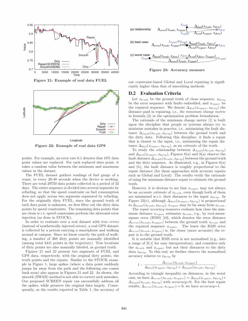
0.7

0.75

0.8

0.85

0.9

0.95

0 5000 10000 15000 20000 25000 30000 35000 40000

Val

ue

Time

Repair

Dirty

Smooth

DirtyRepair(SCREEN)

Smooth(SWAB)

Figure 21: Example of real data FUEL

Latit

ude

Longitude

DirtyRepair

SmoothTruth

Figure 22: Example of real data GPS

points. For example, an error rate 0.1 denotes that 10% datapoint values are replaced. For each replaced data point, ittakes a random value between the minimum and maximumvalues in the dataset.The FUEL dataset gathers readings of fuel gauge of a

crane, in every 20-40 seconds when the device is working.There are total 29750 data points collected in a period of 32days. The entire sequence is divided into several segments byrefueling, so that the speed constraint on fuel consumptiondoes not apply across two segments separated by refueling.For the originally dirty FUEL, since the ground truth ofeach data point is unknown, we first filter out the dirty datapoints by speed constraints. The remaining data points thatare clean w.r.t. speed constraints perform the aforesaid errorinjection (as done in STOCK).In order to evaluate over a real dataset with true errors

(instead of synthetically injected errors), a real GPS datasetis collected by a person carrying a smartphone and walkingaround at campus. Since we know exactly the path of walk-ing, a number of 368 dirty points are manually identified(among total 3441 points in the trajectory). True locationsof dirty points are also manually labeled, as ground truth.Figures 21 and 22 present two segments of FUEL and

GPS data, respectively, with the original dirty points, thetruth points and the repairs. Similar to the STOCK exam-ple in Figure 1, large spikes (where a data point suddenlyjumps far away from the path and the following one comesback soon) also appear in Figures 21 and 22. As shown, thesmooth (SWAB) method is not able to correct such mistakes.Our proposed SCREEN repair can successfully address allthe spikes, while preserve the original data largely. Conse-quently, as the results reported in Table 1, the accuracy of

Figure 23: Accuracy measure

our constraint-based Global and Local repairing is signifi-cantly higher than that of smoothing methods.

D.2 Evaluation CriteriaLet xtruth be the ground truth of clean sequence, xdirty

be the error sequence with faults embedded, and xrepair bethe repaired sequence. We denote Δdist(xrepair, xdirty) thedistance paid in repairing, i.e., the minimum change metricin formula (2) in the optimization problem formulation.

The rationale of the minimum change metric [1] is builtupon the discipline that people or systems always try tominimize mistakes in practice, i.e., minimizing the fault dis-tance Δfault(xtruth, xdirty) between the ground truth andthe dirty data. Following this discipline, it finds a repairthat is closest to the input, i.e., minimizing the repair dis-tance Δdist(xrepair, xdirty), as an estimate of the truth.

To study the relationship between Δfault(xtruth, xdirty)and Δdist(xrepair, xdirty), Figures 8(a) and 9(a) observe thefault distance Δfault(xtruth, xdirty) between the ground truthand the dirty sequence. As illustrated, e.g., in Figures 8(a)and (b), the fault distance is roughly proportional to therepair distance (for those approaches with accurate repairssuch as Global and Local). The results verify the rationaleof using the minimum distance repair to estimate the groundtruth.

However, it is obvious to see that xrepair may not alwaysbe an accurate estimate of xtruth, even though both of themare minimized w.r.t. their distances to the input xdirty. InFigure 23(c), although Δdist(xrepair, xdirty) is proportionalto Δfault(xtruth, xdirty), xrepair may be far away from xtruth.The repair accuracy measures evaluate how close the min-

imum distance xrepair estimates xtruth, e.g., by root-mean-square error (RMS) [10], which denotes the error distanceΔerror(xtruth, xrepair) between the ground truth xtruth andthe repaired sequence xrepair. The lower the RMS errorΔerror(xtruth, xrepair) is, the closer (more accurate) the re-pair is to the ground truth.

It is notable that RMS error is not normalized (e.g., intoa range of [0,1] for easy interpretation), and considers onlythe xtruth and xrepair but not their distances to the dirtydata xdirty. To this end, we further observe the normalizedaccuracy relative to xdirty by

1− Δerror(xtruth, xrepair)

Δdist(xrepair, xdirty) + Δfault(xtruth, xdirty),

According to triangle inequality on distances, in the worstcase, we have Δerror(xtruth, xrepair) = Δdist(xrepair, xdirty)+Δfault(xtruth, xdirty) with accuracy=0. For the best repairresults, Δerror(xtruth, xrepair) = 0, we have accuracy=1.

841