
Screen-Space Far-Field Ambient Obscurance - wiliwili.cc/research/ffao/ffao.pdf · Screen-Space...
11
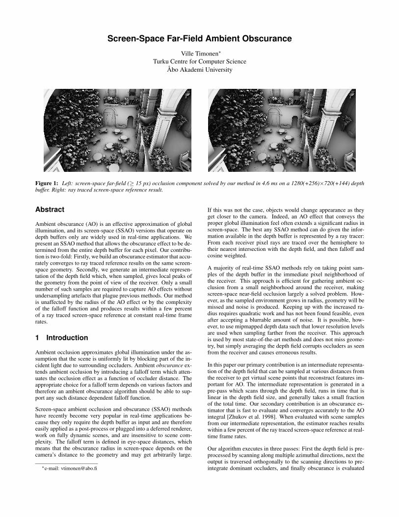
Screen-Space Far-Field Ambient Obscurance Ville Timonen * Turku Centre for Computer Science Åbo Akademi University Figure 1: Left: screen-space far-field (≥ 15 px) occlusion component solved by our method in 4.6 ms on a 1280(+256)×720(+144) depth buffer. Right: ray traced screen-space reference result. Abstract Ambient obscurance (AO) is an effective approximation of global illumination, and its screen-space (SSAO) versions that operate on depth buffers only are widely used in real-time applications. We present an SSAO method that allows the obscurance effect to be de- termined from the entire depth buffer for each pixel. Our contribu- tion is two-fold: Firstly, we build an obscurance estimator that accu- rately converges to ray traced reference results on the same screen- space geometry. Secondly, we generate an intermediate represen- tation of the depth field which, when sampled, gives local peaks of the geometry from the point of view of the receiver. Only a small number of such samples are required to capture AO effects without undersampling artefacts that plague previous methods. Our method is unaffected by the radius of the AO effect or by the complexity of the falloff function and produces results within a few percent of a ray traced screen-space reference at constant real-time frame rates. 1 Introduction Ambient occlusion approximates global illumination under the as- sumption that the scene is uniformly lit by blocking part of the in- cident light due to surrounding occluders. Ambient obscurance ex- tends ambient occlusion by introducing a falloff term which atten- uates the occlusion effect as a function of occluder distance. The appropriate choice for a falloff term depends on various factors and therefore an ambient obscurance algorithm should be able to sup- port any such distance dependent falloff function. Screen-space ambient occlusion and obscurance (SSAO) methods have recently become very popular in real-time applications be- cause they only require the depth buffer as input and are therefore easily applied as a post-process or plugged into a deferred renderer, work on fully dynamic scenes, and are insensitive to scene com- plexity. The falloff term is defined in eye-space distances, which means that the obscurance radius in screen-space depends on the camera’s distance to the geometry and may get arbitrarily large. * e-mail: vtimonen@abo.fi If this was not the case, objects would change appearance as they get closer to the camera. Indeed, an AO effect that conveys the proper global illumination feel often extends a significant radius in screen-space. The best any SSAO method can do given the infor- mation available in the depth buffer is represented by a ray tracer: From each receiver pixel rays are traced over the hemisphere to their nearest intersection with the depth field, and then falloff and cosine weighted. A majority of real-time SSAO methods rely on taking point sam- ples of the depth buffer in the immediate pixel neighborhood of the receiver. This approach is efficient for gathering ambient oc- clusion from a small neighborhood around the receiver, making screen-space near-field occlusion largely a solved problem. How- ever, as the sampled environment grows in radius, geometry will be missed and noise is produced. Keeping up with the increased ra- dius requires quadratic work and has not been found feasible, even after accepting a blurrable amount of noise. It is possible, how- ever, to use mipmapped depth data such that lower resolution levels are used when sampling farther from the receiver. This approach is used by most state-of-the-art methods and does not miss geome- try, but simply averaging the depth field corrupts occluders as seen from the receiver and causes erroneous results. In this paper our primary contribution is an intermediate representa- tion of the depth field that can be sampled at various distances from the receiver to get virtual scene points that reconstruct features im- portant for AO. The intermediate representation is generated in a pre-pass which scans through the depth field, runs in time that is linear in the depth field size, and generally takes a small fraction of the total time. Our secondary contribution is an obscurance es- timator that is fast to evaluate and converges accurately to the AO integral [Zhukov et al. 1998]. When evaluated with scene samples from our intermediate representation, the estimator reaches results within a few percent of the ray traced screen-space reference at real- time frame rates. Our algorithm executes in three passes: First the depth field is pre- processed by scanning along multiple azimuthal directions, next the output is traversed orthogonally to the scanning directions to pre- integrate dominant occluders, and finally obscurance is evaluated
Transcript of Screen-Space Far-Field Ambient Obscurance - wiliwili.cc/research/ffao/ffao.pdf · Screen-Space...
Screen-Space Far-Field Ambient Obscurance
Ville Timonen∗
Turku Centre for Computer ScienceÅbo Akademi University
Figure 1: Left: screen-space far-field (≥ 15 px) occlusion component solved by our method in 4.6 ms on a 1280(+256)×720(+144) depthbuffer. Right: ray traced screen-space reference result.
Abstract
Ambient obscurance (AO) is an effective approximation of globalillumination, and its screen-space (SSAO) versions that operate ondepth buffers only are widely used in real-time applications. Wepresent an SSAO method that allows the obscurance effect to be de-termined from the entire depth buffer for each pixel. Our contribu-tion is two-fold: Firstly, we build an obscurance estimator that accu-rately converges to ray traced reference results on the same screen-space geometry. Secondly, we generate an intermediate represen-tation of the depth field which, when sampled, gives local peaks ofthe geometry from the point of view of the receiver. Only a smallnumber of such samples are required to capture AO effects withoutundersampling artefacts that plague previous methods. Our methodis unaffected by the radius of the AO effect or by the complexityof the falloff function and produces results within a few percentof a ray traced screen-space reference at constant real-time framerates.
1 Introduction
Ambient occlusion approximates global illumination under the as-sumption that the scene is uniformly lit by blocking part of the in-cident light due to surrounding occluders. Ambient obscurance ex-tends ambient occlusion by introducing a falloff term which atten-uates the occlusion effect as a function of occluder distance. Theappropriate choice for a falloff term depends on various factors andtherefore an ambient obscurance algorithm should be able to sup-port any such distance dependent falloff function.
Screen-space ambient occlusion and obscurance (SSAO) methodshave recently become very popular in real-time applications be-cause they only require the depth buffer as input and are thereforeeasily applied as a post-process or plugged into a deferred renderer,work on fully dynamic scenes, and are insensitive to scene com-plexity. The falloff term is defined in eye-space distances, whichmeans that the obscurance radius in screen-space depends on thecamera’s distance to the geometry and may get arbitrarily large.
∗e-mail: [email protected]
If this was not the case, objects would change appearance as theyget closer to the camera. Indeed, an AO effect that conveys theproper global illumination feel often extends a significant radius inscreen-space. The best any SSAO method can do given the infor-mation available in the depth buffer is represented by a ray tracer:From each receiver pixel rays are traced over the hemisphere totheir nearest intersection with the depth field, and then falloff andcosine weighted.
A majority of real-time SSAO methods rely on taking point sam-ples of the depth buffer in the immediate pixel neighborhood ofthe receiver. This approach is efficient for gathering ambient oc-clusion from a small neighborhood around the receiver, makingscreen-space near-field occlusion largely a solved problem. How-ever, as the sampled environment grows in radius, geometry will bemissed and noise is produced. Keeping up with the increased ra-dius requires quadratic work and has not been found feasible, evenafter accepting a blurrable amount of noise. It is possible, how-ever, to use mipmapped depth data such that lower resolution levelsare used when sampling farther from the receiver. This approachis used by most state-of-the-art methods and does not miss geome-try, but simply averaging the depth field corrupts occluders as seenfrom the receiver and causes erroneous results.
In this paper our primary contribution is an intermediate representa-tion of the depth field that can be sampled at various distances fromthe receiver to get virtual scene points that reconstruct features im-portant for AO. The intermediate representation is generated in apre-pass which scans through the depth field, runs in time that islinear in the depth field size, and generally takes a small fractionof the total time. Our secondary contribution is an obscurance es-timator that is fast to evaluate and converges accurately to the AOintegral [Zhukov et al. 1998]. When evaluated with scene samplesfrom our intermediate representation, the estimator reaches resultswithin a few percent of the ray traced screen-space reference at real-time frame rates.
Our algorithm executes in three passes: First the depth field is pre-processed by scanning along multiple azimuthal directions, next theoutput is traversed orthogonally to the scanning directions to pre-integrate dominant occluders, and finally obscurance is evaluated

per-pixel from the reconstructed occluders. The key features of ourSSAO solution are:
• Constant time, unbounded radius (the effect may span the en-tire screen)
• Does not miss important occluders (no noise or need to filter)
• Supports arbitrary falloff functions (no render time evalua-tion)
2 Previous work
In this section we cover only previous work most relevant for ourmethod; for a recent review of ambient occlusion and SSAO meth-ods, consult [Ritschel et al. 2012].
The main branch of present SSAO methods follows from the worksof [Mittring 2007] and [Shanmugam and Arikan 2007] where pointsamples around the receiver are taken to approximate the visibil-ity of the hemisphere. In order to avoid overocclusion when sam-ples farther from the receiver are evaluated, it is important to knowwhether there is intersecting geometry closer to the receiver whichwould render the sampled point invisible. To this end, it is possi-ble to connect the samples along one azimuthal direction to get onehorizon value instead, as done in [Bavoil et al. 2008]. AO is calcu-lated based on the global horizon angle and rays below the horizonare assumed to be occluded. However in ambient obscurance, whena non-constant falloff term is used, occluders’ distances below thehorizon affect the amount of occlusion and need to be known. Ourmethod tracks the horizon incrementally as geometry is traversedoutwards from the receiver, and occlusion coming from geometryvisible to the receiver below the global horizon is properly weightedby distance.
Global horizons for a height field are calculated efficiently in [Ti-monen and Westerholm 2010] for direct lighting of a height field,however for ambient obscurance the same single-horizon problemapplies: No information is kept of the geometry below the globalhorizon, and weighting the occlusion properly according to a fallofffunction is not possible. Errors can get arbitrarily large because it isnot known how far the geometry below the global horizon is fromthe receiver. [Timonen 2013] fits this method to SSAO by find-ing the largest falloff attenuated occluder for each direction insteadof the global horizon. While this is much more useful for SSAO,geometry above the largest occluder is ignored and the distance tothe geometry below the largest occluder is still unknown. Whilethis is suitable for approximate SSAO, results do not converge toa ray traced reference or scale to very high quality like those ofour method. Also, both [Timonen and Westerholm 2010] and [Ti-monen 2013] sample the height field along straight lines whereaswe account for the visibility of the geometry over the full azimuth.Considering geometry only along a set of straight lines significantlyaccentuates banding (cf. Figure 10).
Lower resolution (mipmapped) depth buffers can be used for sam-pling farther from the receiver as done by [Bavoil and Sainz 2009][Hoang and Low 2012] [McGuire et al. 2012]. An artefact-freesampling of this multi-resolution representation is not a trivial task,as shown in [Snyder and Nowrouzezahrai 2008]. Regardless of theused low-pass filter, reducing the depth field over an area into asingle-valued texel does not capture the view-dependency when thedepth field is viewed from an arbitrary receiver. While we also usea resolution hierarchy, we capture information of the enclosed ge-ometry such that it retains the approximated local peaks as viewedfrom any receiver. Furthermore, levels in our hierarchy are well-aligned (do not overlap or have gaps), making artefact-free sam-pling straight-forward.
Methods that sample an area around the receiver that is fixed inscreen-space may produce fast results [Loos and Sloan 2010], butthese methods neither scale to far-field AO nor respect a falloffterm. It is also possible to use a forward rendering approach to AOwhereby scene geometry prior to rendering is expanded and occlu-sion is spread onto the area of influence. This approach is pursuedin [McGuire 2010], but the method does not scale to far-field effectsbecause of increased overocclusion and high fillrate requirements.
A near-field screen-space search can be coupled with a far-fieldworld-space method. A voxelization of the scene is ray tracedin [Reinbothe et al. 2009], and [Shanmugam and Arikan 2007]use spherical proxies to approximate scene polygons. World-spacemethods have significantly different characteristics to screen-spacemethods: While they have the possibility to include geometry notvisible in the depth buffer, they are forced to evaluate the visibilityof many geometric primitives per pixel. This is costly and proneto produce overocclusion. Results and performance depend on thescene geometry whereas pure screen-space methods are insensitiveto scene complexity.
Finally, purely ray traced AO methods such as [Laine and Karras2010] produce results similar in quality to ours but do not sufferfrom the limitations of screen-space information. These methodsare, however, at least an order of magnitude slower.
3 Algorithm overview
Our algorithm takes as input the depth and normal buffers, the pro-jection matrix, and a pointer to the falloff function. The depth andnormal buffers can change freely between frames, and the depthbuffer may include optional guard bands. Geometry within theguard bands are considered as occluders, but obscurance values arenot calculated for pixels in the guard band. The output of our algo-rithm is a floating point map of the ambient light.
We evaluate the 2D ambient obscurance integral in K azimuthalslices. In Section 4 we describe our obscurance estimator that isevaluated for each screen pixel. It takes scene points along eachazimuthal direction as input. In order to generate these points, ourmethod first scans the depth buffer in parallel lines in K azimuthaldirections and writes out an intermediate representation at regularlyspaced intervals along the lines as described in detail in Section 6.This is illustrated for one azimuthal direction to the left in Figure 2.This intermediate data is then optionally (when the depth field canbe assumed continuous) traversed perpendicular to the azimuthalscan direction and turned into a prefix sum, as shown to the centerin Figure 2. The purpose of the prefix sum is to allow averaging ofthe intermediate data over each of the K azimuthal sectors whicheffectively avoids azimuthal undersampling and reduces banding.This phase is described in Section 7. Finally, the prefix sum issampled per pixel, shown to the right in Figure 2, to construct points(as input to our obscurance estimator) that track local peaks of thedepth field. As a reference method we use a mipmapped depthbuffer, described in Section 5, which is used in present state-of-the-art. Results are presented in Section 8.
The remaining perceptually dominant artefact in our method isbanding. We propose three mutually complementary strategies toreduce banding:
1. Averaging scene points over sectors in continuous depth fields(Section 7)
2. Sparse evaluation of sectors which trades banding for blur andreduces render times (Section 10)
3. Jittering sampling directions per-pixel which trades bandingfor noise (Section 11.1)
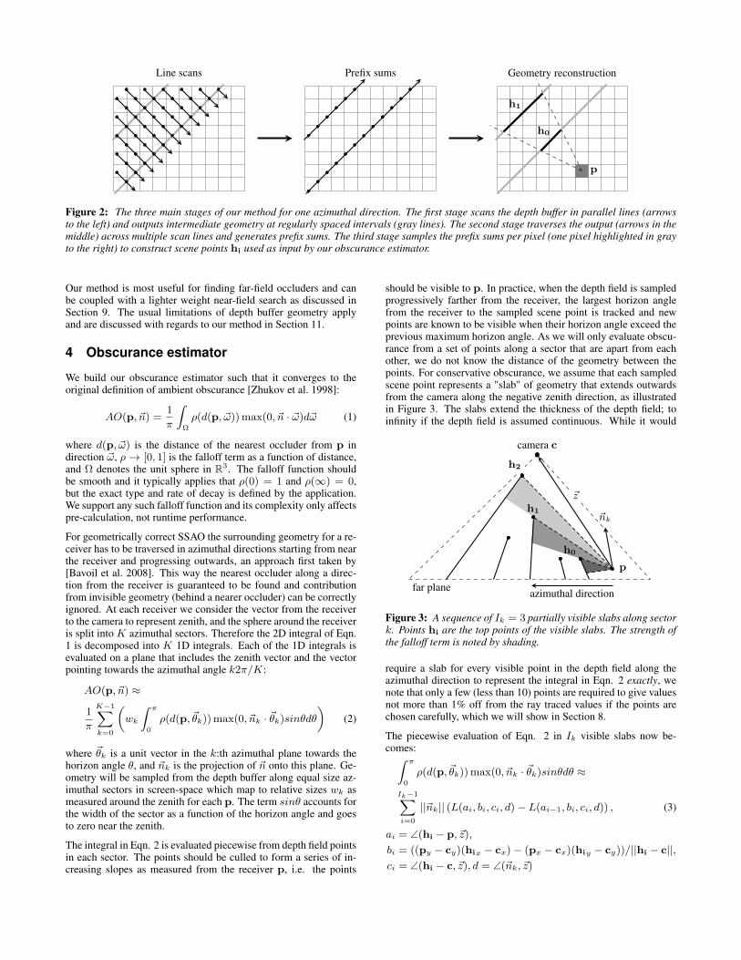
Line scans Prefix sums Geometry reconstruction
p
h0
h1
Figure 2: The three main stages of our method for one azimuthal direction. The first stage scans the depth buffer in parallel lines (arrowsto the left) and outputs intermediate geometry at regularly spaced intervals (gray lines). The second stage traverses the output (arrows in themiddle) across multiple scan lines and generates prefix sums. The third stage samples the prefix sums per pixel (one pixel highlighted in grayto the right) to construct scene points hi used as input by our obscurance estimator.
Our method is most useful for finding far-field occluders and canbe coupled with a lighter weight near-field search as discussed inSection 9. The usual limitations of depth buffer geometry applyand are discussed with regards to our method in Section 11.
4 Obscurance estimator
We build our obscurance estimator such that it converges to theoriginal definition of ambient obscurance [Zhukov et al. 1998]:
AO(p, ~n) =1
π
∫
Ω
ρ(d(p, ~ω))max(0, ~n · ~ω)d~ω (1)
where d(p, ~ω) is the distance of the nearest occluder from p indirection ~ω, ρ → [0, 1] is the falloff term as a function of distance,and Ω denotes the unit sphere in R
3. The falloff function shouldbe smooth and it typically applies that ρ(0) = 1 and ρ(∞) = 0,but the exact type and rate of decay is defined by the application.We support any such falloff function and its complexity only affectspre-calculation, not runtime performance.
For geometrically correct SSAO the surrounding geometry for a re-ceiver has to be traversed in azimuthal directions starting from nearthe receiver and progressing outwards, an approach first taken by[Bavoil et al. 2008]. This way the nearest occluder along a direc-tion from the receiver is guaranteed to be found and contributionfrom invisible geometry (behind a nearer occluder) can be correctlyignored. At each receiver we consider the vector from the receiverto the camera to represent zenith, and the sphere around the receiveris split into K azimuthal sectors. Therefore the 2D integral of Eqn.1 is decomposed into K 1D integrals. Each of the 1D integrals isevaluated on a plane that includes the zenith vector and the vectorpointing towards the azimuthal angle k2π/K:
AO(p, ~n) ≈
1
π
K−1∑
k=0
(
wk
∫ π
0
ρ(d(p, ~θk))max(0, ~nk · ~θk)sinθdθ
)
(2)
where ~θk is a unit vector in the k:th azimuthal plane towards thehorizon angle θ, and ~nk is the projection of ~n onto this plane. Ge-ometry will be sampled from the depth buffer along equal size az-imuthal sectors in screen-space which map to relative sizes wk asmeasured around the zenith for each p. The term sinθ accounts forthe width of the sector as a function of the horizon angle and goesto zero near the zenith.
The integral in Eqn. 2 is evaluated piecewise from depth field pointsin each sector. The points should be culled to form a series of in-creasing slopes as measured from the receiver p, i.e. the points
should be visible to p. In practice, when the depth field is sampledprogressively farther from the receiver, the largest horizon anglefrom the receiver to the sampled scene point is tracked and newpoints are known to be visible when their horizon angle exceed theprevious maximum horizon angle. As we will only evaluate obscu-rance from a set of points along a sector that are apart from eachother, we do not know the distance of the geometry between thepoints. For conservative obscurance, we assume that each sampledscene point represents a "slab" of geometry that extends outwardsfrom the camera along the negative zenith direction, as illustratedin Figure 3. The slabs extend the thickness of the depth field; toinfinity if the depth field is assumed continuous. While it would
camera c
far planeazimuthal direction
p
~z
~nk
h2
h1
h0
Figure 3: A sequence of Ik = 3 partially visible slabs along sectork. Points hi are the top points of the visible slabs. The strength ofthe falloff term is noted by shading.
require a slab for every visible point in the depth field along theazimuthal direction to represent the integral in Eqn. 2 exactly, wenote that only a few (less than 10) points are required to give valuesnot more than 1% off from the ray traced values if the points arechosen carefully, which we will show in Section 8.
The piecewise evaluation of Eqn. 2 in Ik visible slabs now be-comes:
∫ π
0
ρ(d(p, ~θk))max(0, ~nk · ~θk)sinθdθ ≈
Ik−1∑
i=0
||~nk|| (L(ai, bi, ci, d)− L(ai−1, bi, ci, d)) , (3)
ai = ∠(hi − p, ~z),
bi = ((py − cy)(hix − cx)− (px − cx)(hiy − cy))/||hi − c||,
ci = ∠(hi − c, ~z), d = ∠(~nk, ~z)

where L is a 4D pre-calculated table. The four arguments of L, inorder, are
1. The angle ai of the vector from the receiver to the sampledscene point
2. The closest distance bi from the receiver to the line formed bythe slab, hi + t(hi − c)
3. The angle ci of the slab
4. The angle d of the projected normal
where all angles are with respect to the zenith vector ~z = c− p. Lis constructed in an offline pre-pass by generating the correspond-ing slabs and evaluating the falloff weighted integral numerically byray casting. We have implemented L as a 3D texture where ci and dshare an axis. The sharing is implemented by first splitting the axisinto segments, one for each discretized value of d, and then placingconsecutive values of ci consecutively within each segment. There-fore ai, bi, and ci can be linearly interpolated and d is chosen as thenearest discretized value. Although L is of high dimensionality, theinvolved functions are very smooth and therefore low resolutionsare sufficient which helps to keep the texture size moderate (withina few MB).
5 Reference method: mipmap
Our obscurance estimator needs as input the scene points alongazimuthal directions in the depth buffer for each receiver. In thesimplest case these points can be direct depth buffer samples de-projected into eye-space. While this is the most widely taken ap-proach in current SSAO methods, it does not scale well to far-field:Dense sampling translates into high render times and sparse sam-pling causes undersampling artefacts because important geometrymight be missed.
The approach taken by previous state-of-the-art SSAO methods isto generate a depth pyramid (mipmap) that has a series of lowerresolution levels of the depth buffer. Regardless of the filter usedto generate the lower resolution levels from the base level, this ap-proach does not retain the view-dependent information of the depthfield necessary for accurate AO. We tried several filters includingthe ones covered in [McGuire et al. 2012] and considered averagingto produce the best results as it does not introduce sudden changesto obscurance like, for example, max-mipmaps do. However, whenthe depth field cannot be assumed continuous, only points in theoriginal depth buffer can be used. In this case we found max-mipmaps to perform best and we use them in Section 11. UntilSection 11 we assume a continuous depth field and compare ourgeometry representation against averaged mipmaps.
In the mipmap method, from each receiver point, we start traversingthe surrounding depth buffer along each of the K azimuthal direc-tions by first sampling the base level texture at a distance of onetexel. After each sample, the step size is multiplied by a constantand the sampling distance is accumulated by the step size. Thisyields an exponentially sparser sampling. We found the constantof 1.5 to produce the best performance-quality tradeoff when usedwith K = 16 and these parameters are used in Section 8.
We use trilinear filtering available in hardware, and choose themipmap level in such a way that the sample’s coverage of the depthbuffer matches the sector’s width at any given sampling distance.In order to avoid sudden changes in obscurance when the last sam-pling position goes outside the depth buffer, an extra sample is al-ways taken at the very edge of the depth buffer.
6 Intermediate geometry along scanlines
In this section we describe how our method scans the depth bufferin order to create an intermediate representation of the depth field.We scan the depth buffer in a dense set of parallel lines for each Kazimuthal direction and incrementally track the depth field profilealong those lines. The parallel lines are spaced one texel width apartalong the depth buffer and the lines are traversed one texel widthstep at a time. In a threaded implementation one thread processesone line. A scan along one azimuthal direction in a depth buffer isshown to the left in Figure 4.
m0
m0
Figure 4: The depth buffer (grid shown in the background) isscanned in one of the K azimuthal directions in parallel lines (ar-rows). The maximum height m0 of each line every B0 = 3 steps(thick gray lines) is written to a buffer holding the intermediatedata. Progression along one line is shown to the right.
We base our method on the intuition that points important for AOare local peaks in the depth field. To track these local peaks, wefind the highest (nearest to the camera) depth field points along thelines. In practice, we step through each line incrementally and ateach point we sample the depth buffer and deproject the scene pointinto eye-space. The maximum height value is then rememberedalong the line until B0 steps have been taken. After B0 steps themaximum height is written into an intermediate geometry bufferand reset. This is illustrated to the right in Figure 4. The process isrepeated until the end of the depth buffer.
However, which local peak has the highest contribution to AO isdependent on the angle at which the receiver views the peak. Themaximum height value is guaranteed to represent the highest hori-zon value for a receiver that is at the same height, i.e. when thepeak is viewed directly horizontally. However, receivers (pointsalong the line) may reside at various heights and therefore view thedepth field peaks from different angles. Instead of storing the maxheight value as viewed directly horizontally, we store 2 max heightvalues: one as viewed horizontally (mo) and one as viewed at adownwards angle (m1). We call the angles along which the maxheight values are viewed receiver angles. This is illustrated to theleft in Figure 5.
During the evaluation of the obscurance estimator the intermediategeometry buffer is read and a virtual point is reconstructed at theintersection of the receiver angles as shown to the right in Figure5. Intuitively this virtual point is a view-dependent (for a likely re-ceiver) approximation of the highest peak within the interval of B0
steps along the scanning line. After culling the invisible points perreceiver, these points can be directly used as hi by the obscuranceestimator in Eqn. 3.
We have chosen to use slopes 0 (horizontal) and -1 (45 degreesdownward) for the receiver angles. We found that the choice for thereceiver angles does not make a large difference to results, howeverit is important that there are two different angles such that the recon-structed virtual point will have both a depth and a distance value.Algorithm 1 lists the pseudocode for scanning one line in the depthbuffer.

m1
m0
m0
m1
m0
m0
m1
m1
h1
h0
Figure 5: The maximum heights (denoted by m0 and m1) asviewed along 2 receiver angles are written to the intermediatebuffer every B0 = 3 steps. The virtual points (hi) as geometryused by the obscurance estimator are reconstructed at the intersec-tion of the corresponding receiver angles positioned at m0 and m1,as shown to the right.
Algorithm 1 ScanLine(float2 pos, float2 dir, int steps, int lineNo)Pos is the coordinate of the first step in the depth buffer and dir is avector for one step along the scanline.
1 float m0 = −∞2 float m1 = −∞34 while (steps−−)5 6 float3 p = deProj(sampleDepth(pos), pos)7 // p is projected onto k:th azimuthal plane8 float2 pk = (p.xy · dir, p.z)9
10 m0 = max(m0, pk.y)11 // s = slope of the downwards receiver angle (−1)12 m1 = max(m1, pk.y + s·pk.x)1314 if (steps modulo B0 == 0)15 16 // iBuf = the intermediate buffer (output of this stage)17 iBuf[lineNo][steps/B0] = (m0, m1)18 m0 = −∞19 m1 = −∞20 2122 pos += dir23
Algorithm 2 lists the pseudocode for evaluating obscurance at onescreen pixel along one azimuthal direction. Since SSAO is sep-arable in azimuthal directions, Algorithms 1 and 2 can be calcu-lated sequentially for each K, in which case our method requiresO(W0 ·H0/B0) space for the intermediate geometry buffer, whereW0 and H0 are the depth buffer dimensions including guard bands.For a typical case of W0 = 1280+256, H0 = 720+144, B0 = 10this is roughly 1 MB. If the application is not memory constrainedit is faster to evaluate Algorithm 1 for all K simultaneously as tomaximize the number of concurrent threads and therefore improveutilization of a GPU. For K = 16 the respective memory require-ment becomes 16.2 MB.
The accuracy of our intermediate geometry becomes progressivelybetter compared to mipmaps when the interval size increases. Dueto the falloff function occluders far from the receiver get less weightand also map to smaller swaths of the horizontal angle than nearbyoccluders. Therefore it is sensible to construct occluders progres-sively more sparsely when farther from the receiver. Similarly
Algorithm 2 EvalObscurance(float2 pixelPos, float2 dir)
1int lineNo = find the line with direction dir closest to pixelPos2int iVal = find the nearest interval in lineNo that is at least B0
steps from pixelPos34float3 p = deProj(sampleDepth(pixelPos), pixelPos)5// zScale scales z onto the slanted azimuthal plane
6float zScale =√
1 + (p.x/p.z · dir.y − p.y/p.z · dir.x)27float2 pk = (p.xy · dir, p.z·zScale)89float (AO, maxAngle) =
EvalNearField(pixelPos, dir, distance to iVal)1011while (iVal ≥ 0) 12float (m0,m1) = iBuf[lineNo][iVal]13// s = slope of the downwards receiver angle14float2 h = ((m0 − m1)/s, m0·zScale)15float angle = ∠((h − pk),−~pk) // c is at the origin16if (angle > maxAngle)1718// Obs(ai, ai-1, hi, p) evaluates i:th segment from Eqn. 319AO += Obs(angle, maxAngle, h, pk)20maxAngle = angle2122iVal−−232425return AO
to building multiple resolutions of the depth field in the form ofmipmaps, our intermediate geometry can be made into a 1D pyra-mid. We form levels of the intermediate geometry such that theirintervals increase exponentially from the base level’s, B0. There-fore the interval of level n is Bn = B0 · 2
n. The levels can be effi-ciently generated by taking the max m0 and m1 from the two cor-responding lower level intervals. Generating the exponential hier-archy roughly doubles the required space but reduces the per-pixeltime complexity from O(n) to O(log(n)) where n is the pixel dis-tance from the receiver to the edge of the depth buffer.
7 Averaging sectors
In Section 6 we described how to construct virtual points for theobscurance estimator defined in Section 4 from geometry along asingle line in the depth buffer. We propose this approach when itis not possible to average or interpolate depth field values, which isthe case in Section 11 where the depth field is assumed to representa volume of a finite thickness. In this section we assume that thedepth field is continuous and averaging is thereby allowed.
Ideally the virtual points should represent the entire sector insteadof the thin texel wide line along the center of the azimuthal sec-tor. The sector’s width increases linearly in the distance from thereceiver as demonstrated in Figure 6. In Figure 6 lines contribut-ing to the obscurance at p are shown as arrows. The horizontalintervals are equal to the gray lines perpendicular to the scanningdirection previously shown to the left in Figure 4. In order to con-struct the averaged point for the highlighted middlemost intervalshown in Figure 6, we simply average m0 and m1 over the par-allel lines lA...lB fitting into the sector at that specific distance:(ma
0 ,ma1) = 1/(lB − lA + 1) · ΣlB
li=lAiBuf[li][iV al]. When the
virtual point is constructed (line 14 in Algorithm 2) ma0 and ma
1 areused instead of m0 and m1. In order to calculate the average in

B0
B0
B0
p
lBlAiBuf[li][iV al]
Figure 6: The downward arrows denote scan lines along one az-imuthal scanning direction. Lines indexed li ∈ [lA, lB ] at the high-lighted interval (constant index iV al) fit into the sector from re-ceiver p and their m0 and m1 should be averaged.
constant time, we turn the buffer iBuf into a per-interval prefix sumiBufP such that iBufP [li][iV al] = Σli
l=0iBuf[l][iV al]. From the
prefix sum the average over any line range l0...l1 for interval iV alcan then be efficiently calculated as (iBufP [l1][iV al]− iBufP [l0 −1][iV al])/(l1 − l0 + 1).
We therefore introduce another stage between Algorithm 1 and 2which traverses the intermediate geometry buffer iBuf perpendicu-larly to the scan direction in Algorithm 1 and accumulates m0 andm1 values over lines. This stage produces the prefix summed ver-sion iBufP which can, in fact, be built in-place over the originaliBuf.
Finally, when evaluating obscurance, instead of averaging the inter-vals across the entire sector width, the obscurance can be evaluatedin multiple segments to increase azimuthal resolution. While doingso does not produce results quite as accurate as if the number ofsectors K is increased by a corresponding factor, evaluating a sec-tor in multiple segments is computationally lighter than increasingthe number of sectors and has the same effect on reducing banding.More importantly, evaluation in multiple segments does not requireextra azimuthal scans over the depth buffer. We have chosen to spliteach sector in half and evaluate obscurance in 2 segments per sec-tor. From now on, we denote this by adding a multiplier to K, e.g.K = 8× 2 for eight azimuthal directions and two segments.
8 Results
We ran our algorithm on AMD Radeon HD 7970(OpenCL) and NVIDIA GeForce GTX 580 (CUDA).Sources are available under the BSD license online athttp://wili.cc/research/ffao/. The mipmapmethod using our obscurance estimator and Horizon-Based Am-bient Occlusion (HBAO) [Bavoil et al. 2008] are implemented asOpenGL fragment shaders. Performance and quality comparisonbetween other recent SSAO methods can be found in [Vardis et al.2013] and [McGuire 2010].
Our algorithm calculates the far-field SSAO in 3 kernels:
1. The Scan kernel scans through the depth buffer in K az-imuthal scanning directions in parallel lines and finds localpeaks of the depth field at regularly spaced intervals.
2. The Prefix sum kernel reads through the values over multi-ple lines in a direction perpendicular to the scan direction andgenerates prefix sums.
3. The Obscurance kernel reconstructs virtual points from theprefix sums that are averaged over the azimuthal sector width
at each screen pixel. The final obscurance value per pixelis calculated by evaluating the obscurance estimator with thevirtual points.
We have chosen two scenes as our main test material. The firstscene is an architectural scene with simple planar geometry (Figure7, top), and the second scene shows complex geometry and foliage(Figure 7, bottom). The scenes are rendered using exponentiallydecreasing falloff functions whereby in the first scene the fallofffunction decays slower than in the second scene. All renderingsuse a 10% guard band (extending 10% of the visible framebufferwidth or height at each side) which is denoted by postfixing it tothe resolution in parentheses.
For our method we use K = 8 × 2 and K = 16 × 2 and for themipmap method we use K = 16. As reference we use ray trac-ing on the same geometry (a single-layer depth buffer with a 10%guard band). In the ray traced result rays with cosine-weighted di-rections are cast around the hemisphere for each receiver pixel, andstepped through in small steps until geometry is being intersected.The intersection distance is then weighted by the falloff functionand accumulated to the result. This can arguably be considered thebest result any method can do with the available screen-space data.
In addition to difference images, we measure the error using twometrics: eA measures the average per-pixel variation from the raytraced values and e<5% measures the number of pixels within 5%of the ray traced values. A high value in e<5% denotes that onlyfew pixels behave abnormally, which also implies temporal stabilitysince the reference values do not wave or flicker. In Figure 7 wehave rendered the two scenes using our method and the mipmapmethod and compared the results against the ray tracing.
Recall that our obscurance estimator conservatively assumes ascene point to represent a slab of geometry which extends alongthe negative zenith. However, actual depth field geometry betweenslabs can be closer to the receiver. The error coming from the over-estimated distance is relative to the density of the slabs, which wein this section keep constant at roughly 8 slabs per azimuthal di-rection. The average error introduced by this in the first scene iseA ≈ 0.6% and in the second scene eA ≈ 0.8%, which sets alower bound for the error as K is increased. Obscurance as esti-mated from the geometry produced by our method is very accurateeven when a low number of sectors is being used, mainly becausethe evaluated virtual scene points are tailored to capture the fea-tures of the scene geometry that specifically contribute to AO. Themipmap method is inadequate in capturing the "profile" of the ge-ometry within the sample’s radius and produces erroneous results.Furthermore, the mipmap method converges to the ray traced val-ues very slowly: It takes over 300 ms to achieve the same level oferror as in our method at K = 8× 2 and several seconds to matchK = 16× 2.
While the quantitative error in our method is small, there can stillbe banding that is perceptually prominent. The level of banding de-pends on the geometric content: Bands are cast by sharp tall edgesand are visible on planar surfaces. Averaging the virtual points overthe widths of each sector reduces banding, especially from occlud-ers far from the receiver where the banding is almost completelyremoved. Banding is discussed in more detail in Section 10. Tem-poral coherence can be a major concern in SSAO methods that ex-hibit undersampling, whereas the dense azimuthal scans employedby our method do not skip geometry. Overall we observe that theresults of our method look temporally stable (under motion) whichis to be expected given the small variation with respect to the stableray traced values.
In comparison, Figure 8 shows results as rendered by HBAO us-ing the same falloff function. HBAO does not assume a continuous

Our, K = 8× 2
error×5
eA = 1.17%, e<5% = 98.9%
Our, K = 16× 2
error×5
eA = 0.92%, e<5% = 99.8%
Mipmap, K = 16
error×5
eA = 8.63%, e<5% = 25.8%
Ray traced
error×5
eA = 1.92%, e<5% = 93.3%
error×5
eA = 1.27%, e<5% = 98.5%
error×5
eA = 9.90%, e<5% = 38.9%
Figure 7: Two scenes rendered by our method and the mipmap method and their respective error images (white = 0%, black ≥ 20%, brighteris better), average error (eA, lower is better) and the number of pixels within 5% (e<5%, higher is better) of the ray traced reference.
depht field. Instead, it assumes that geometry between two con-secutive visible points along an azimuthal direction is at the samedistance from the receiver as the higher of the two visible points.As HBAO’s obscurance estimator is not built to converge to Eqn. 1results look dissimilar to the ray traced reference. HBAO requiresvery many samples per pixel to cover far-field effects accuratelywhich shows up as impractically high render times.
Let W0×H0 be the resolution of the depth buffer with guard bands,and W ×H without. Then the time complexity of our method forkernel 1 is O(K ·W0 ·H0), for kernel 2 O(K ·W0 ·H0/B0), andfor kernel 3 O(K ·W ·H · log(W0+H0)). We consider the scalingfavorable, as the per-pixel cost increases only logarithmically in theresolution while the full depth field is still considered for each pixel.
Our method is insensitive to the geometric content of the depthbuffer and the obscurance radius has no effect on the render times;obscurance is gathered from the entire guard banded depth bufferfor every pixel. Table 1 lists the total execution time of the secondscene in Figure 7 for our method and for the mipmap method usingtwo different GPUs and two common screen resolutions. All tim-ings only include far-field AO, which starts at approximately 1.5B0
pixels from the receiver. The same far-field boundary is used forboth methods.
Table 2 shows how the execution time is split between the threestages of our method. In the Obscurance kernel, we measure theaverage number of constructed virtual points to be 7.8 per sector
Table 1: Total render times of the far-field AO component.
Method Radeon 7970 GTX 5801280(+256)× 720(+144), B0 = 10:Our, K = 8× 2 7.26 ms 12.0 msOur, K = 16× 2 13.3 ms 23.6 msMipmap, K = 16 19.2 ms 17.7 ms1920(+384)× 1080(+216), B0 = 10:Our, K = 8× 2 16.7 ms 29.4 msOur, K = 16× 2 31.6 ms 58.1 msMipmap, K = 16 31.5 ms 37.9 ms
per pixel. The mipmap method takes an average of 8.5 samples persector per pixel.
Table 2: Render time breakdown of our method per kernel.
Phase Radeon 7970 GTX 5801280(+256)× 720(+144), K = 8× 2, B0 = 10:Scan 0.537 ms 0.489 msPrefix sum 0.945 ms 0.617 msObscurance 5.77 ms 10.9 ms

12×48 samples per pixel, 81 ms
error×5
12×32 samples per pixel, 43 ms
error×5
Figure 8: Scenes from Figure 7 as rendered by HBAO on aGeForce GTX 580 at 1280(+256)×720(+144). Obscurance is cal-culated in K = 12 azimuthal directions that are randomly rotatedper pixel.
9 Integration with near-field
From a time complexity point of view our method is effective intreating near-field obscurance as well, however our method’s ben-efits become significant only when the geometry enclosed by theinterval Bi covers a large distance. In order to bring the nearestinterval in our method closer to the receiver, B0 has to be reduced,which increases the execution time and the memory footprint. Wesuggest that our method be combined with a lightweight near-fieldsearch that gathers obscurance from an area around the receiver thatis at least a couple of pixels in radius. Where exactly the boundarybetween the near-field and our method should be depends on thecharacteristics of the near-field search: Our method should gener-ally take over at a distance where the near-field method is no longerfaster. The interval of the base level, B0, determines the nearestdistance at which our method can take over. Halving B0 causesone extra interval per sector to be evaluated (roughly a constant in-crease in execution time), and reduces the area of influence of thenear-field search to quarter. Table 3 lists our method’s executiontimes for different values of B0.
Table 3: Far-field render times of our method using different valuesfor the base level interval B0.
Base level Radeon 7970 GTX 5801280(+256)× 720(+144), K = 8× 2:B0 = 20 6.06 ms 9.77 msB0 = 10 7.26 ms 12.0 msB0 = 5 8.89 ms 14.7 ms
When integrating a near-field method with our method, the near-field method should be executed first and provide the maximumhorizon angles from the near-field range along the K sectors foreach pixel as shown at line 9 in Algorithm 2. After this, our method
continues accumulating the obscurance from the horizon angle up-wards until the edge of the depth field. We expect B0 ∈ [5, 10] tobe a suitable choice for a typical state-of-the-art near-field search.Figure 9 shows the contribution of the far-field and the near-fieldobscurance components on a 720p depth buffer using B0 = 10.
+
=
Figure 9: The far-field component (≥ 15 px) as produced by ourmethod and the near-field component (< 15 px) together form thefinal ambient obscurance result (bottom).
10 Banding
While the error in our method is small, as established in Section 8,there still might be some visible banding even though we averageoccluders across the width of a sector. In order to gain intuition onwhy banding happens, consider the case where an occluder—say,a wall—enters an otherwise flat sector in a linear motion. If thesector was split into infinitely many subsectors, obscurance wouldincrease linearly as the wall occupied a larger swath of the sector.In our method, the entering wall increases the average height ofan interval linearly, which might not map to linear change in ob-scurance. This is especially evident for very tall occluders whichcause the obscurance value to increase faster than linearly whenonly a small portion of the occluder is occupying the sector. So,while the obscurance values at band boundaries in our method donot jump abruptly, they don’t follow the physically correct curveeither. In Figure 10 we show a split screen of a scene rendered us-ing K = 8× 2 averaged sectors as described in Section 7 and thenusing K = 16 straight sampling lines that go through the centerline of each sector. Averaging eliminates far-field banding almostcompletely, which is often the hardest to rid, but near-field bandingstill persists.
One solution to the banding problem is to increase the number ofscanning directions K which shows up as a roughly linear increasein execution times of the Scan and Prefix sum stages. Instead ofevaluating all K sectors for every pixel, it is possible to evaluate thesectors sparsely. We use the Separable Approximation of AmbientOcclusion (SAAO) approach from [Huang et al. 2011], and evaluateK = 18 × 2 sectors in groups of 3 × 3 pixels. Obscurance istherefore evaluated in an interleaved pattern such that only K =2 × 2 sectors are evaluated per pixel and the results are gatheredusing an edge-aware 3 × 3 box filter as a post-process. Any 3 × 3pixel neighborhood includes all K = 18 × 2 sectors and thereforeno noise is produced to the image. SAAO produces errors primarilyat edges and depth discontinuities in the depth buffer. While thefar-field AO component can also change by unbounded amounts

Figure 10: Left: our method using K = 8 × 2 averaged sectors.Right: our method using K = 16 straight sampling lines.
between adjacent pixels in the screen, the error is mainly in thenear-field.
We have incorporated SAAO in our method by combining a 3 × 3separated far-field AO with a full near-field AO. The primary arte-facts are small integration errors (noise) at the boundary of the far-field and near-field AO components because they are of differentsparsity. The error can be hidden to a large extent by a selectiveblur that uses a small intensity threshold and does not currupt theimage. In Figure 11 a result without blurring is shown to the right,which shows minor noise, and the image to the left includes a 5×5bilateral box blur. Figure 1 is also rendered using the method shownto the left.
Figure 11: Our method using K = 18 × 2 with SAAO. Left:selectively blurred result. Right: result without blurring.
We implement SAAO by introducing two new kernels:
Box average kernel is an edge-aware filter which averages depthand the normal vectors from a 3 × 3 pixel neighborhood ofeach framebuffer pixel. If the dot product of the normal of thesource pixel and the candidate pixel is higher than 0.5 and therelative difference of pixel depths is below 3%, the pixel isaccepted into the average. The accepted pixels are the pixelsfrom which the far-field obscurance is gathered in the Gatherkernel, and therefore a bit mask representing the accepted pix-els is carried to the Gather kernel. The averaged depth andnormal vectors are used in the Obscurance kernel instead ofthe original pixel’s values.
Gather kernel combines the per-pixel near-field obscurance withan average of the far-field obscurance from pixels that weremarked as accepted in Box average kernel. Results are op-tionally blurred using a bilateral box filter of size 5 × 5 witha threshold of 7% (pixels within a maximum of 7% color dif-ference are included into the average).
The SAAO enabled render times are shown in Table 4. The execu-
Phase Radeon 7970 GTX 580K = 18× 2 (3× 3 separation), B0 = 10,1280(+256)× 720(+144):Scan 1.07 ms 1.08 msPrefix sum 1.09 ms 1.04 msBox average 0.265 ms 0.400 msObscurance, sep. 1.60 ms 3.00 msGather (with blur) 0.255 (0.591) ms 0.290 (0.652) mstotal (with blur) 4.28 (4.62) ms 5.81 (6.17) ms1920(+384)× 1080(+216):Scan 2.32 ms 3.08 msPrefix sum 2.03 ms 2.08 msBox average 0.566 ms 0.894 msObscurance, sep. 3.82 ms 7.25 msGather (with blur) 0.557 (1.31) ms 0.651 (1.46) mstotal (with blur) 9.29 (10.0) ms 14.0 (14.8) ms
Table 4: Render time breakdown of our method per kernel withSAAO enabled.
tion time of the Obscurance kernel decreases linearly in the num-ber of evaluated sectors. In fact, the Scan and Prefix sum kernelsnow take more time than the Obscurance kernel in some cases, andspeeding up these two kernels would be the logical next step in im-proving the execution times and is briefly discussed in Section 13.Overall, SAAO is an efficient way to trade banding for noise or blurwhile also improving render times significantly.
11 Limitations of depth buffer geometry
Scene geometry in a depth buffer is incomplete in two ways: (i)geometry outside the view frustum is unknown and (ii) geometrybelow the first depth layer is unknown. The first limitation is usu-ally addressed by introducing a guard band around the depth buffer.In this paper we have used a guard band of 10% (extending thedepth buffer by 10% of its width or height in each direction). Asthe screen-space radius of the obscurance effect may become arbi-trarily large when scene geometry is close to the camera, it cannotbe entirely contained within a guard band in any SSAO method.However, the slower the decay of the falloff function the larger theguard band generally needs to be and thus becomes important toour method. Fortunately the Z pre-pass is usually quick and lowerresolution rasterization can be used in the guard bands to furtherminimize its cost. As long as the Z pre-pass does not have a highcost, we recommend even larger than 10% guard bands when calcu-lating far-field AO effects in screen-space. It is also possible to con-struct a simplified world-space representation of occluders aroundthe camera that are outside the depth buffer and accumulate SSAOwith occlusion from them using a global AO method, however thisapproach is outside the scope of this paper
Most SSAO methods use only a single depth layer and make ageneric assumption about the geometry below the nearest depthlayer. Such an approach can never produce correct results in allscenes and the artefacts vary. Until this section we have assumedthe depth field to be continuous, i.e. an infinitely thick volume.This has the benefits, for example, that depth field points can beaveraged and interpolated, and objects appearing behind nearer ge-ometry within the view frustum will not cause abrupt changes to ob-scurance. The downside is that obscurance is often overestimated,and to a large degree if there are thin objects, such as chains hang-ing in the air, near the camera. Because we in this paper advocate ahigh quality and physically correct SSAO, we find more promise inapproaches that attempt to fill the missing scene geometry with real

information of the scene instead of fitting a scene-dependent as-sumption. In previous work such information has been introducedin the form of multiple depth layers [Bavoil and Sainz 2009] andmultiple views [Vardis et al. 2013]. Extending our method into thatdirection is left as future work.
Instead, we briefly demonstrate our method under the assumptionthat the depth field has a fixed finite thickness, an approach taken bymany prior works such as [Loos and Sloan 2010] [McGuire et al.2011] [McGuire et al. 2012]. While this will not work for arbi-trary views or scenes that have varied objects, it produces plausi-ble results when the depth field thickness is carefully selected andmatches that of the viewed objects. Fixing the thickness requiresa small change in the obscurance estimator in Eqn. 3: ai−1 is re-placed with max(ai−1,∠(hi+ t(hi−c)/||hi−c||−p, ~z)) wheret is the thickness of the depth field.
When the depth field thickness is finite the depth field becomesdiscontinuous. Therefore it is not allowed to generate new pointsthrough interpolation or averaging. This limitation does not muchimpact direct depth buffer samples which can be snapped to texelcenters as done in [Bavoil et al. 2008]. In our method this meansthat averaging across the sector’s width as described in Section 7cannot be used, however we still retain the advantage over directsamples that our method tracks the local peaks along each samplingline. The mipmap method, however, is most impacted: Not only isinterpolation spatially and across mip levels forbidden, but lowerresolution level textures have to reuse values found from the baselevel and no averaging is possible. Out of various filters we foundmax-mipmaps to produce best results for mipmapping.
In Figure 12 we show the Stanford Dragon as rendered by our ob-scurance estimator with a fixed depth field thickness using our inter-mediate geometry samples, direct depth buffer samples, and max-mipmaps. All methods evaluate roughly 8 far-field samples per az-imuthal direction. SAAO is not used. Direct depth field samplesand our method produce banding especially since sector averag-ing cannot be used for mitigation. Therefore our method does notuse the Prefix sum stage and reconstructs scene points as per Al-gorithm 1 and 2 directly. Our method produces smooth obscurancealong each azimuthal direction whereas direct depth buffer samplesproduce artefacts depending on whether the samples hit or miss lo-cal peaks in the depth field. Due to the missed geometry, directsampling also produces systematic underocclusion. Max-mipmapsdo not miss geometry but systematically overestimate it by alwayspicking the largest occluder within the sample’s radius. Also, aslinear interpolation cannot be used the results are blocky.
11.1 Jittering
It is possible to jitter the sampling directions per-pixel to tradebanding for noise. In our method this can be achieved by addingor substracting an offset value from the sampled line indices lA andlB shown in Figure 6. The offset is randomly selected per pixel, andsampling along every direction is offset by the same amount as notto cause bias. The offset is scaled according to the distance fromthe receiver to the interval. Here, when averaging is not allowedand only a single line is sampled along each azimuthal direction,banding becomes especially severe if jittering is not used. Over-all we find that jittering the sampling direction within the sectorboundaries efficiently eliminates banding in return for some noise.Our method is the cache-friendliest of the three methods with re-spect to jittering because neighboring pixels access the same inter-vals which are laid out in memory consecutively and accesses arelikely to hit the same cache lines. Mipmapping exhibits better cachelocality than the sparser direct samples and its render times are notimpacted significantly by jittering.
12 Conclusion
We have presented a method to solve ambient obscurance in screen-space from occluders that are beyond the immediate neighborhoodof the receiving pixel. We do this by first scanning the depth bufferin a number of azimuthal directions while tracking local heightmaxima and writing them into an intermediate geometry buffer.After creating prefix sums of the intermediate geometry buffer, itcan be sampled per-pixel to obtain approximated local peaks in theenvironment as seen from the receiver point, at various distances.These reconstructed scene points are then evaluated using an obscu-rance estimator to approximate the AO integral over the receiver’shemisphere. The obscurance effect in our method is only limitedby the falloff term, and our method can incorporate any such termwithout its evaluation affecting render times. Overall our method isable to produce very high quality AO effects that are close to a raytraced screen-space reference.
The intended use for our algorithm is to couple it with a lightweightnear-field search to build a robust SSAO solution that accuratelyintegrates ambient obscurance from the entire guard banded depthbuffer.
13 Future work
Currently we scan the depth buffer densely, which is justifiablesince the Obscurance stage takes most of the execution time and isnot impacted by scanning density. However, a dense scan becomescostly when SAAO is used as a significant amount of the total timeis spent in the Scan and Prefix sum stages that scale linearly in thenumber of scanned lines. It is possible to leave out some of theparallel lines during azimuthal scans without much impact on thecalculated obscurance because the lines are always approximatelyfacing the receiver and therefore have a limited contribution to AO.Ideally, processing every n:th line reduces the execution time of theScan and Prefix sum stages by the factor 1/n.
Overall there are four main strategies to reduce the render time ofour method:
• Sparse scans as described above
• Separated obscurance evaluation sparser than 3×3 (which isused in Section 10), such as 5×5
• Reducing K and increasing the number of segments in whicheach sector is evaluated (e.g. K = 8× 4)
• Constructing fewer points (larger intervals) per azimuthal di-rection per pixel.
We are also investigating the possibility of extending our methodto handle multiple depth layers [Bavoil and Sainz 2009] or mul-tiple views [Vardis et al. 2013] which—when coupled with suffi-ciently large guard bands—would alleviate the screen-space prob-lem of missing scene geometry. This could allow our method toproduce results comparable to global ray tracing.
References
BAVOIL, L., AND SAINZ, M. 2009. Multi-layer dual-resolutionscreen-space ambient occlusion. In SIGGRAPH ’09 Talks, ACM.
BAVOIL, L., SAINZ, M., AND DIMITROV, R. 2008. Image-spacehorizon-based ambient occlusion. In SIGGRAPH ’08 Talks.
HOANG, T.-D., AND LOW, K.-L. 2012. Efficient screen-space ap-proach to high-quality multiscale ambient occlusion. The VisualComputer 28, 3, 289–304.

Our method
No jittering (16.3 ms) Jittered (19.1 ms)
eA = 1.18%
Direct samples
No jittering (16.8 ms) Jittered (38.8 ms)
eA = 2.12%
Max-mipmaps
No jittering (14.8 ms) Jittered (19.8 ms)
eA = 3.84%
error×5 error×5 error×5
Figure 12: The Stanford Dragon rendered in K = 16 azimuthal directions with a hand-picked thickness t using our intermediate geometry(left), direct depth buffer samples (middle), and max-mipmaps (right). The right side of each image uses azimuthal directions that arerandomly jittered per-pixel. The resolution is 1280(+256)×720(+144) and the render times are reported for the far-field (B0 = 10) AOcomponent on a GeForce GTX 580.
HUANG, J., BOUBEKEUR, T., RITSCHEL, T., HOLLÄNDER, M.,AND EISEMANN, E. 2011. Separable approximation of ambientocclusion. In Eurographics 2011 - Short papers.
LAINE, S., AND KARRAS, T. 2010. Two methods for fast ray-castambient occlusion. CGF: Proceedings of EGSR 2010 29, 4.
LOOS, B. J., AND SLOAN, P.-P. 2010. Volumetric obscurance. InProceedings of I3D 2010, ACM.
MCGUIRE, M., OSMAN, B., BUKOWSKI, M., AND HENNESSY,P. 2011. The alchemy screen-space ambient obscurance algo-rithm. In Proc. HPG, ACM, HPG ’11, 25–32.
MCGUIRE, M., MARA, M., AND LUEBKE, D. 2012. Scalableambient obscurance. In High-Performance Graphics 2012.
MCGUIRE, M. 2010. Ambient occlusion volumes. In Proceedingsof High Performance Graphics 2010.
MITTRING, M. 2007. Finding next gen: Cryengine 2. In SIG-GRAPH ’07: ACM SIGGRAPH 2007 courses, ACM, 97–121.
REINBOTHE, C., BOUBEKEUR, T., AND ALEXA, M. 2009. Hy-brid ambient occlusion. EUROGRAPHICS 2009 Areas Papers.
RITSCHEL, T., DACHSBACHER, C., GROSCH, T., AND KAUTZ,J. 2012. The state of the art in interactive global illumination.Computer Graphics Forum 31 (Feb.).
SHANMUGAM, P., AND ARIKAN, O. 2007. Hardware acceleratedambient occlusion techniques on gpus. In Proc. I3D ’07, ACM.
SNYDER, J., AND NOWROUZEZAHRAI, D. 2008. Fast soft self-shadowing on dynamic height fields. Computer Graphics Fo-rum: Eurographics Symposium on Rendering (June).
TIMONEN, V., AND WESTERHOLM, J. 2010. Scalable HeightField Self-Shadowing. Computer Graphics Forum (Proceedingsof Eurographics 2010) 29, 2 (May), 723–731.
TIMONEN, V. 2013. Line-Sweep Ambient Obscurance. ComputerGraphics Forum (Proceedings of EGSR 2013) 32, 4.
VARDIS, K., PAPAIOANNOU, G., AND GAITATZES, A. 2013.Multi-view ambient occlusion with importance sampling. InProc. i3D, I3D ’13, 111–118.
ZHUKOV, S., INOES, A., AND KRONIN, G. 1998. An Ambi-ent Light Illumination Model. In Rendering Techniques ’98,Springer-Verlag Wien New York, G. Drettakis and N. Max, Eds.,Eurographics, 45–56.