Scotland's Rural College

WTI and Brent futures pricing structure

Scheitrum, DP; Carter, CA; Revoredo-Giha, C

Published in:Energy Economics

DOI:10.1016/j.eneco.2018.04.039

First published: 26/04/2018

Document VersionPeer reviewed version

Link to publication

Citation for pulished version (APA):Scheitrum, DP., Carter, CA., & Revoredo-Giha, C. (2018). WTI and Brent futures pricing structure. EnergyEconomics, 72, 462 - 469. https://doi.org/10.1016/j.eneco.2018.04.039

General rightsCopyright and moral rights for the publications made accessible in the public portal are retained by the authors and/or other copyright ownersand it is a condition of accessing publications that users recognise and abide by the legal requirements associated with these rights.

• Users may download and print one copy of any publication from the public portal for the purpose of private study or research. • You may not further distribute the material or use it for any profit-making activity or commercial gain • You may freely distribute the URL identifying the publication in the public portal ?

Take down policyIf you believe that this document breaches copyright please contact us providing details, and we will remove access to the work immediatelyand investigate your claim.

Download date: 12. Feb. 2022

WTI and Brent Futures Pricing Structure

Daniel P. Scheitruma,∗, Colin A. Carterb, Cesar Revoredo-Gihac

aThe University of Arizona, Tucson, AZ 85721

bUniversity of California, Davis, One Shields Avenue, Davis, CA 95616

cScotland’s Rural College (SRUC), Kings Buildings, West Mains Road, Edinburgh EH9 3JG, UK

Abstract

WTI and Brent crude oil futures are competing pricing benchmarks and they jockey for the

number one position as the leading futures market. The price spread between WTI and Brent

is also an important benchmark itself as the spread affects international trade in oil, refiner

margins, and the price of refined products globally. In addition, the shapes of the WTI and

Brent futures curves reflect supply and demand fundamentals in the U.S. versus the world

market, respectively.

On the analysis of the relationship between the two futures prices, we identify a

structural break in the WTI–Brent price spread in January 2011 and a break in the corre-

sponding shapes of the futures curves around the same time. The structural break was a

consequence of a dramatic rise in U.S. production due to fracking, a series of supply dis-

ruptions in Europe, binding storage constraints, and the U.S. crude oil export ban. These

events are studied in the context of a simulation model of world oil prices. We reproduce

the stylized facts of the oil market and conclude that the 2011 break in pricing structure was

consistent with standard commodity storage theory.

Keywords: crude oil futures, commodity storage, WTI, Brent, competitive storage model

∗Corresponding author: dpscheitrum@email.arizona.edu.

Preprint submitted to Elsevier April 16, 2018

1. Introduction1

The crude oil futures market is dominated by two competing benchmark grades,2

West Texas Intermediate (WTI) and Brent crude. As benchmarks, WTI and Brent provide a3

reference price against which oil around the world is traded at a premium or discount. WTI4

is primarily traded on the NYMEX (CME Group) while Brent is primarily traded on the5

Intercontinental Exchange (ICE). The CME Group and ICE both cross list WTI and Brent.6

However, the CME accounts for over 80% of WTI volume and the ICE accounts for about7

90% of the Brent trading volume.8

The pricing point for WTI is delivery into either a pipeline or storage facility in9

Cushing, Oklahoma. Brent crude specifies delivery onto a vessel at the Sullom Voe oil termi-10

nal on the Shetland Islands in the North Sea. The chemical characteristics of Brent and WTI11

are nearly identical, with Brent crude being the slightly less sulfurous of the two. Annual12

trading volume for each of the contracts is displayed in Figure 1 where it is shown that for13

three recent years (2012-2014) Brent displaced WTI as the most heavily traded oil futures14

market. During this time period, the U.S. government’s Energy Information Administra-15

tion (EIA) abandoned WTI for its reference oil price, and substituted the North Sea Brent16

contract, in its 2013 Annual Energy Outlook. The reasoning was that WTI was somewhat17

disconnected from the global market. At the time Brent was a superior benchmark because18

imported crude into the eastern and western U.S. coastal markets and refined products in the19

U.S. are priced off the global market. But shifting to Brent as a reference price was not ideal20

because oil production in the North Sea is dwindling due to aging oil fields in that region.21

Crude oil sold in the U.S. is priced off the WTI contract, while oil sold internationally22

is typically priced off Brent. Therefore the spread between the two is a very important metric23

in the global oil complex. The spread reflects the competitiveness of U.S. in the world market24

and in addition the WTI–Brent price spread is an indicator of refiner profitability in the U.S.25

2

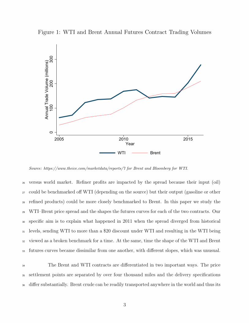
Figure 1: WTI and Brent Annual Futures Contract Trading Volumes

010

020

030

0An

nual

Tra

de V

olum

e (m

illion

s)

2005 2010 2015Year

WTI Brent

Source: https://www.theice.com/marketdata/reports/7 for Brent and Bloomberg for WTI.

versus world market. Refiner profits are impacted by the spread because their input (oil)26

could be benchmarked off WTI (depending on the source) but their output (gasoline or other27

refined products) could be more closely benchmarked to Brent. In this paper we study the28

WTI–Brent price spread and the shapes the futures curves for each of the two contracts. Our29

specific aim is to explain what happened in 2011 when the spread diverged from historical30

levels, sending WTI to more than a $20 discount under WTI and resulting in the WTI being31

viewed as a broken benchmark for a time. At the same, time the shape of the WTI and Brent32

futures curves became dissimilar from one another, with different slopes, which was unusual.33

The Brent and WTI contracts are differentiated in two important ways. The price34

settlement points are separated by over four thousand miles and the delivery specifications35

differ substantially. Brent crude can be readily transported anywhere in the world and thus its36

3

spot price is more correlated with port and coastal grades of crude oil (The Intercontinental37

Exchange, 2013). Alternatively, WTI is more responsive to U.S.-specific supply and demand38

fundamentals and infrastructure issues. Further, the WTI pricing point is co-located with39

substantial above-ground storage, 73 million barrels of storage capacity (EIA, 2016c). The40

Brent location is more of a just-in-time production model with only 8.4 million barrels of41

available storage (Olsen, 2012, BP, 2016). Conceptually, the vastly different storage facilities42

could give rise to alternative inter-temporal price spreads in one market versus the other.43

The law of one price suggests that the spot prices for these nearly equivalent grades of crude44

oil should differ by no more than the transactions costs of transporting oil from one market45

to another. This is why the spot prices were so closely linked prior to 2011, when the U.S.46

was a major net importer of oil (Fattouh, 2010).47

Inter-temporal prices are linked through storage (Working, 1949, Brennan, 1958,48

Wright and Williams, 1982) and spatial prices are linked by trade (Makki, Tweeten and49

Miranda, 1996, Miranda and Glauber, 1995). There have been other cases in the commodities50

space where the law of one price has broken down, but typically, these are short lived events.51

For instance, in early 2014 natural gas prices at the Algonquin citygate hub serving Boston52

reached about $25 per mmBTU compared to $5 per mmBTU in Henry Hub due to pipeline53

capacity constraints (EIA, 2016b). However, this price differential lasted only a matter of54

months compared to the lengthy WTI–Brent differential.55

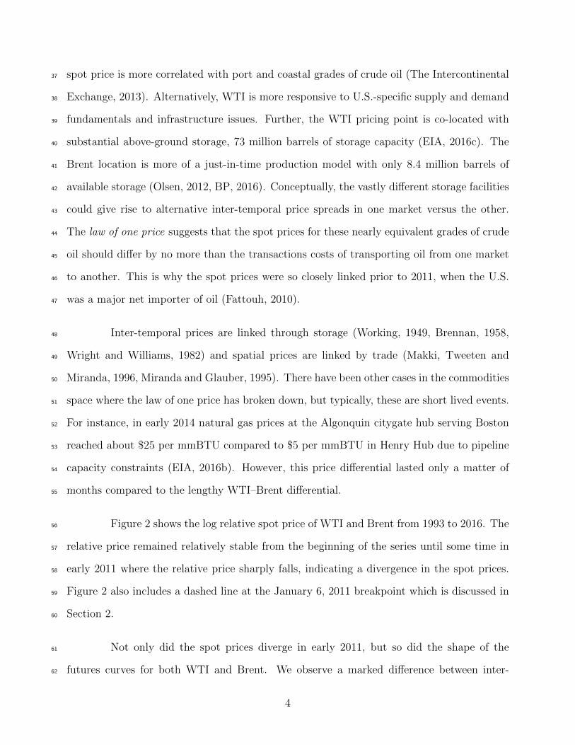
Figure 2 shows the log relative spot price of WTI and Brent from 1993 to 2016. The56

relative price remained relatively stable from the beginning of the series until some time in57

early 2011 where the relative price sharply falls, indicating a divergence in the spot prices.58

Figure 2 also includes a dashed line at the January 6, 2011 breakpoint which is discussed in59

Section 2.60

Not only did the spot prices diverge in early 2011, but so did the shape of the61

futures curves for both WTI and Brent. We observe a marked difference between inter-62

4

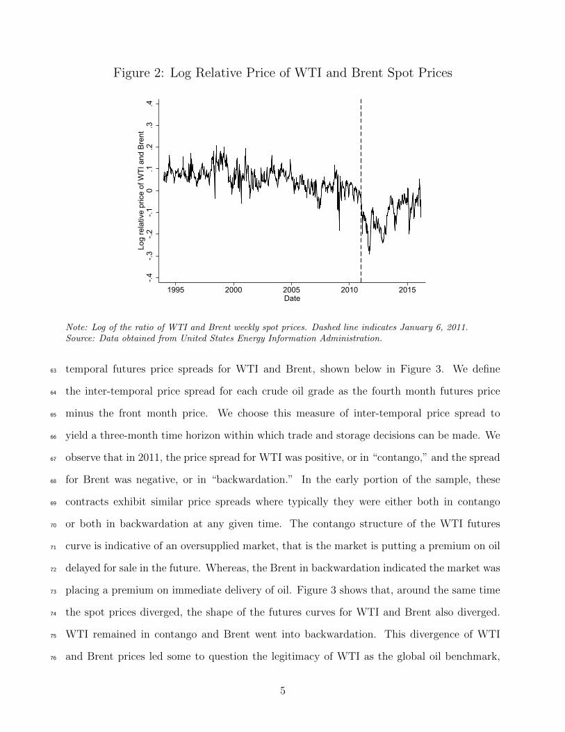
Figure 2: Log Relative Price of WTI and Brent Spot Prices

-.4-.3

-.2-.1

0.1

.2.3

.4Lo

g re

lativ

e pr

ice

of W

TI a

nd B

rent

1995 2000 2005 2010 2015Date

Note: Log of the ratio of WTI and Brent weekly spot prices. Dashed line indicates January 6, 2011.Source: Data obtained from United States Energy Information Administration.

temporal futures price spreads for WTI and Brent, shown below in Figure 3. We define63

the inter-temporal price spread for each crude oil grade as the fourth month futures price64

minus the front month price. We choose this measure of inter-temporal price spread to65

yield a three-month time horizon within which trade and storage decisions can be made. We66

observe that in 2011, the price spread for WTI was positive, or in “contango,” and the spread67

for Brent was negative, or in “backwardation.” In the early portion of the sample, these68

contracts exhibit similar price spreads where typically they were either both in contango69

or both in backwardation at any given time. The contango structure of the WTI futures70

curve is indicative of an oversupplied market, that is the market is putting a premium on oil71

delayed for sale in the future. Whereas, the Brent in backwardation indicated the market was72

placing a premium on immediate delivery of oil. Figure 3 shows that, around the same time73

the spot prices diverged, the shape of the futures curves for WTI and Brent also diverged.74

WTI remained in contango and Brent went into backwardation. This divergence of WTI75

and Brent prices led some to question the legitimacy of WTI as the global oil benchmark,76

5

Figure 3: WTI and Brent, Weekly Three-Month Price Spreads

-10

-50

510

15$

per b

bl

1995 2000 2005 2010 2015Date

WTI 3 Month Spread Brent 3 Month Spread

Note: The three-month price spread is calculated as the futures price for delivery four months in the futureminus the futures price for delivery one month in the future. Dashed line indicates January 6, 2011.Source: Data obtained from Quandl.com.

suggesting that Brent should take its place (Kilian, 2016). However, Kilian (2016) notes that77

Brent suffers from its own drawbacks such as declining North Sea production leading to low78

liquidity, and the continual broadening of the definition of the Brent benchmark to include79

lower grades of crude. Kilian (2016) wrote that it is “unclear whether there remains enough80

oil in the North Sea to sustain a Brent benchmark in the long run” (p. 33).81

We hypothesize that a series of events, beginning in the late 2000s, led to a situation82

where the combined effect was a break in integrated WTI and Brent markets. The shale83

revolution greatly increased U.S. domestic oil production starting in 2008 (Brown and Yucel,84

2013). A thorough overview of the shale revolution can be found in Kilian (2016) and Alquist85

and Guenette (2014). As U.S. production rose, more oil began flowing to Cushing, OK than86

could be refined and then moved via pipeline. Therefore, crude oil stocks in Cushing began to87

climb (Wilmoth, 2012). In March 2011, storage capacity utilization reached 91% in Cushing,88

OK (EIA, 2015).89

6

At the same time, Europe was experiencing negative supply shocks. The Libyan90

Crisis disrupted production and this incident persisted much longer than expected (Meyer,91

2011). Nigerian pipeline sabotage also disrupted supply (Vidal, 2011). In addition, bad92

weather in the North Sea caused production outages (Meyer, 2011). These supply disruptions93

resulted in severe drawdowns of Brent inventories (Blas and Blair, 2011).94

Prior literature has identified the U.S. shale revolution, non-U.S. production disrup-95

tions, U.S. infrastructure and transportation bottlenecks, the U.S. export ban, reweighting96

of the S&P GSCI commodity index in favor of Brent, and the Dow Jones UBS commodity97

index including Brent for the first time, as explanations for the divergence of the WTI and98

Brent prices (Alquist and Guenette, 2014, Buyuksahin et al., 2013, Chen, Huang and Yi,99

2015, Kilian, 2016, Ye and Karali, 2016).100

We develop a stylized, simulation model of world oil prices that we parameterize and101

calibrate to represent the characteristics of the crude oil market before the structural break.102

We impose features of the key stylized facts: positive production shocks in the U.S., negative103

production shocks in Europe, maximum and minimum storage constraints, and a U.S. export104

ban. We then simulate the model and compare the results with the characteristics of the105

oil market before and after the structural break. We are able to successfully reproduce the106

structural break in the oil market.107

This paper is organized as follows: in Section 2, we present stylized facts of the world108

oil market and we test for and identify a break in cointegration between WTI and Brent daily109

spot prices as well as daily nearby futures prices. In Section 3, we present our hypotheses110

as to why there was a structural break. Next, in Section 4 we develop a stylized model of111

world oil prices based upon the competitive storage model employed by Gustafson (1958),112

Wright and Williams (1982), Deaton and Laroque (1992), and the extensions by Miranda113

and Glauber (1995) and Makki, Tweeten and Miranda (1996) which incorporate trade into114

the model. Section 5 presents the results of our simulation of the model and compares them115

7

to the key stylized facts of the oil market following the structural break. Finaly, Section 6116

concludes.117

2. Stylized facts of the world oil market118

Key stylized facts related to the WTI and Brent markets are shown in Table 1.119

When comparing average data for the three years before the 2011 price break to the average120

for the three years following, U.S. production increased by 43% and North Sea production121

decreased by 29%. Storage levels at the WTI pricing terminal increased by 32% and storage122

levels in OECD Europe declined by 4%.1 Exports from the North Sea to the U.S. declined by123

76% and the average spot price premium for WTI over Brent fell from $0.92 to -$11.18. The124

shape of the forward curve also experienced a shift as the percent of trading days that WTI125

was in contango fell from 90% to 69%, whereas for Brent it fell from 92% to 45%.2 In the126

years following the price break, Brent was in backwardation more often than in contango.127

Futures trading volume in the WTI front month contract fell by 19%, whereas the Brent128

front month (the contract for most immediate delivery) trading volume increased by 61%.129

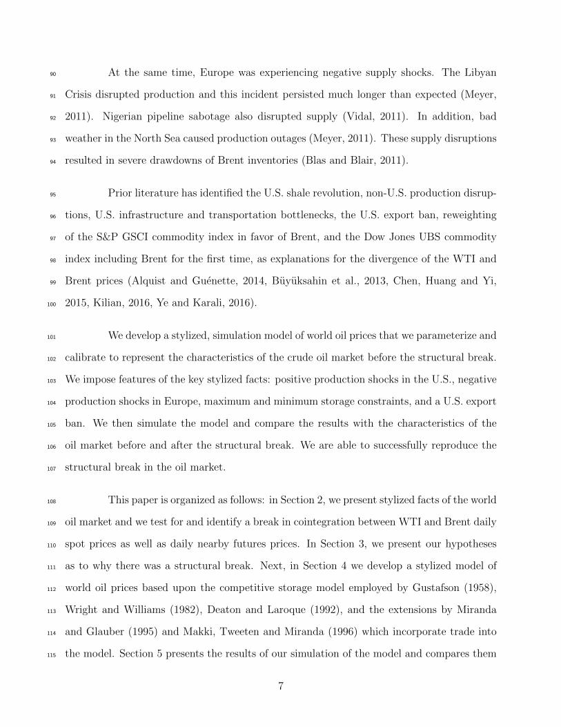
When linked by trade, the spot prices of WTI and Brent crude should be arbitraged.130

Since the inception of the Brent crude benchmark in 1993 through 2011, this was largely131

true. The 52-week rolling correlation between the weekly spot prices of WTI and Brent are132

presented in Figure 4.3 It is apparent that the correlation between these two price series does133

not deviate much from the mean of 0.96 up until some point in 2011 when the relationship134

broke down. The correlation dropped and remained persistently depressed following the start135

1The ideal measure for Brent storage is storage levels at the Sullom Voe terminal, however, these dataare unavailable. As a proxy, storage levels for OECD Europe as a whole declined between these two timeperiods.

2Percent of trading days in contango is measured as the proportion of trading days where the settlementprice for the futures contract four months ahead is greater than the settlement price of the futures contractone month ahead.

3On a given week, the 52-week rolling correlation calculates the correlation between two series for the past52 weeks.

8

Table 1: WTI and Brent Oil Markets, Stylized Facts

2008 - 2010 2012 - 2014 %∆

ProductionU.S. (thousand bbl/day) 5,277 7,546 +43%North Sea (thousand bbl/day) 3,702 2,650 -28%

StorageCushing, OK (thousand bbl) 28,065 37,362 +33%OECD Europe (thousand bbl) 332,333 317,467 -4%

International TradeNorth Sea to U.S. (thousand bbl/day) 140 34 -76%

PricesWTI-Brent Average Spot Premium $0.92 -$11.18 -1,315%

Percent of Trading Days in ContangoWTI 90% 69% -23%Brent 92% 45% -50%

Front Month Trading VolumeWTI 285,591 232,665 -19%Brent 110,570 178,326 +61%

Source: U.S. production data (EIA, 2016f), North Sea production data (EIA, 2016a), Cushing, OK storage

data (EIA, 2016g), and North Sea to U.S. international trade data (EIA, 2016e) are from the U.S. Energy

Information Administration. North Sea production and international trade data are computed as the sum of

country-specific values for Denmark, Germany, the Netherlands, Norway, and the United Kingdom. OECD

Europe storage data are from the IEA Oil Market Reports for February 2012 and February 2016 (IEA,

2012, IEA, 2016). The WTI-Brent average spot premium is calculated as the difference the WTI spot price

minus the Brent spot price per the Energy Information Administration (EIA, 2016d). Percent of trading

days in contango is based on the portion of days where the fourth month futures price exceeds the front

month futures price based on daily futures settle prices for the CME WTI contract and ICE Brent contract

obtained from Quandl.com. Front month trading volume for the CME WTI contract and ICE Brent

contract are based on daily trading volume obtained from Quandl.com.

of 2011. The absolute prices are presented in Figure 5.136

We analyzed the long-term relationship between WTI and Brent series; as they137

were non-stationary4 we tested for cointegration between them using weekly spot prices and138

performing the two-step Engle-Granger test for cointegration (Engle and Granger, 1987). We139

suspect that the two price series are cointegrated during the early portion of our sample, but140

the cointegration degrades at some point. To test for a break in the cointegration between141

4We performed the augmented DF-GLS test on the daily spot prices from 1993 to 2016 and found bothseries non-stationary (Dickey and Fuller, 1979, Elliott, Rothenberg and Stock, 1992). The DF-GLS teststatistic for WTI was -1.577 and for Brent -1.307, therefore it was not possible to reject the hypothesis ofnon-stationarity in levels.

9

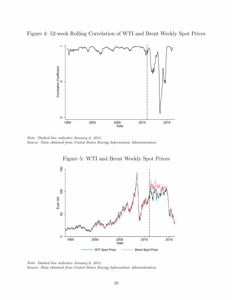
Figure 4: 52-week Rolling Correlation of WTI and Brent Weekly Spot Prices

0.5

1C

orre

latio

n C

oeffi

cien

t

1995 2000 2005 2010 2015Date

Note: Dashed line indicates January 6, 2011.Source: Data obtained from United States Energy Information Administration.

Figure 5: WTI and Brent Weekly Spot Prices

050

100

150

$ pe

r bbl

1995 2000 2005 2010 2015Date

WTI Spot Price Brent Spot Price

Note: Dashed line indicates January 6, 2011.Source: Data obtained from United States Energy Information Administration.

10

WTI and Brent, we perform a supremum Wald test for a structural break at an unknown142

break date using symmetric trimming of 15% in the equation143

WTIt = α + βBrentt + ut (1)

where WTIt is the daily spot price of WTI at time t, and Brentt is the daily spot price of144

Brent at time t. Our test finds a breakpoint on January 6, 2011 which is consistent with145

other studies which have identified December 2010 as the date of a structural break in the146

WTI-Brent price spread (Buyuksahin et al., 2013, Chen, Huang and Yi, 2015, Ye and Karali,147

2016) and in WTI-Brent cointegration (Chen, Huang and Yi, 2015).148

To more formally test for a breakdown in the cointegration between these series, we149

repeat the Engle-Granger cointegration test for the periods before and after the breakpoint.150

We find strong evidence of cointegration between WTI and Brent in the period before the151

January 6, 2011 breakpoint and we fail to reject the hypothesis of no cointegration in the152

period after the breakpoint, at the 1% significance level. Test statistics for the stationarity153

and cointegration tests for the pre- and post-breakpoint periods are presented in Table 2.154

As a robustness check, we test for a structural break in the cointegration of Brent and WTI155

daily spot prices using the Gregory-Hansen test (Gregory and Hansen, 1996). We perform156

the Gregory-Hansen test on Equation 1 allowing for structural change in the level and slope157

of the cointegrating relationship and reject the null hypothesis of no cointegration in favor158

of a structural break on January 10, 2011 at the 1% significance level.159

Turning to the futures market, the 52-week rolling correlation between the front160

month WTI and Brent future prices is reported in Figure 6 and for the fourth month in161

Figure 7. We find statistical evidence of a structural break in the relationship between the162

WTI and Brent front month futures prices on January 6, 2011 as well as between the fourth163

11

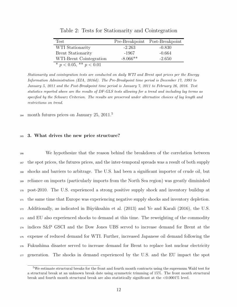
Table 2: Tests for Stationarity and Cointegration

Test Pre-Breakpoint Post-Breakpoint

WTI Stationarity -2.263 -0.830Brent Stationarity -1967 -0.664WTI-Brent Cointegration -8.066** -2.650

* p < 0.05, ** p < 0.01

Stationarity and cointegration tests are conducted on daily WTI and Brent spot prices per the Energy

Information Administration (EIA, 2016d). The Pre-Breakpoint time period is December 17, 1993 to

January 5, 2011 and the Post-Breakpoint time period is January 7, 2011 to February 26, 2016. Test

statistics reported above are the results of DF-GLS tests allowing for a trend and including lag terms as

specified by the Schwarz Criterion. The results are preserved under alternative choices of lag length and

restrictions on trend.

month futures prices on January 25, 2011.5164

3. What drives the new price structure?165

We hypothesize that the reason behind the breakdown of the correlation between166

the spot prices, the futures prices, and the inter-temporal spreads was a result of both supply167

shocks and barriers to arbitrage. The U.S. had been a significant importer of crude oil, but168

reliance on imports (particularly imports from the North Sea region) was greatly diminished169

post-2010. The U.S. experienced a strong positive supply shock and inventory buildup at170

the same time that Europe was experiencing negative supply shocks and inventory depletion.171

Additionally, as indicated in Buyuksahin et al. (2013) and Ye and Karali (2016), the U.S.172

and EU also experienced shocks to demand at this time. The reweighting of the commodity173

indices S&P GSCI and the Dow Jones UBS served to increase demand for Brent at the174

expense of reduced demand for WTI. Further, increased Japanese oil demand following the175

Fukushima disaster served to increase demand for Brent to replace lost nuclear electricity176

generation. The shocks in demand experienced by the U.S. and the EU impact the spot177

5We estimate structural breaks for the front and fourth month contracts using the supremum Wald test fora structural break at an unknown break date using symmetric trimming of 15%. The front month structuralbreak and fourth month structural break are also statistically significant at the <0.0001% level.

12

Figure 6: 52-week Rolling Correlation of WTI and Brent Weekly Front MonthFutures Prices

0.5

1C

orre

latio

n C

oeffi

cien

t

1995 2000 2005 2010 2015Date

Note: Dashed line indicates January 6, 2011.Source: Data obtained from Quandl.com.

Figure 7: 52-week Rolling Correlation of WTI and Brent Weekly FourthMonth Futures Prices

0.5

1C

orre

latio

n C

oeffi

cien

t

1995 2000 2005 2010 2015Date

Note: Dashed line indicates January 25, 2011.Source: Data obtained from Quandl.com.

13

price, futures price, and inter-temporal spread relationships in the same direction as the178

supply shocks. That is, the negative demand shock experienced by the U.S. exacerbates the179

impact of the positive supply shock on the futures pricing relationship. For the EU, the180

positive demand shock exacerbates the impact of the negative supply shock. In Section 5.1,181

we describe an alternative specification of our competitive storage model where we implement182

structural change in the form of demand shifts rather than supply shifts and our results are183

robust to this change in specification.184

The supply shocks in the U.S. and EU oil markets resulted in the price of WTI185

falling below the price of Brent by an amount that far exceeded shipping costs of about $2186

per barrel (Scheid, 2014). The average price difference between 2000 and 2010 had WTI at a187

premium of $1.40 per bbl. The price difference between WTI and Brent reached the extreme188

of WTI at a discount of $29.59 per bbl on September 23, 2011. However, due to the U.S.189

crude oil export ban, this price difference was not arbitraged away. Traders were unable to190

move oil from the United States to Europe or elsewhere to correct the price differential which191

lasted until 2015. As a consequence of the unexpected positive oil supply shocks in the U.S.,192

storage capacity in Cushing, OK reached its maximum. One curious element of the steep193

contango in the United States is that with the relatively new production boom in historically194

non-producing regions (e.g. North Dakota) why would these producers not simply ”store”195

their oil in place rather than extract and deliver into a market that indicate higher prices196

would await in a few months time. Nevertheless, these producers in these regions did extract197

their oil during despite facing a steep contango. When there is no opportunity to put oil into198

storage, it creates pressure to sell immediately thus driving down the spot price relative to199

the futures price. The contrary is true of the Brent market; as unexpected supply disruptions200

persisted and continued to draw down inventories, this put upward pressure on the spot price201

of oil relative to the futures prices. We theorize that had there been no export ban, or if the202

U.S. had plenty of excess storage capacity and Europe had plenty of crude oil in storage, the203

integration of the two markets would have persisted.204

14

4. A stylized model of world oil prices205

As Deaton and Laroque (1992, 1996) employed the competitive storage model to206

reproduce the stylized facts of autocorrelation and price spikes in commodity prices, we207

employ the competitive storage model to reproduce the Brent-WTI oil market pricing struc-208

ture linked by trade. As in Miranda and Glauber (1995), we conceptualize a two-region209

oil market allowing competitive interregional trade, competitive storage, lagged production210

decisions and uncertain output and prices. While a two-region model is a simplification of211

the complex geography of the world oil market, this representation is useful in isolating the212

impacts of barriers to spatial and inter-temporal arbitrage. Since models of trade and storage213

under uncertainty do not have analytical solutions (Gustafson, 1958, Deaton and Laroque,214

1992, Miranda and Glauber, 1995, Gardner, 1979), we solve and simulate the competitive215

storage model numerically using the Rational Expectations Complementarity Solver created216

by Christophe Gouel (2012). In order to capture the nature of the oil market at the time of217

the market pricing anomaly, we impose the restriction on trade that United States may not218

export oil and we impose constraints on storage such that storage levels may not fall below219

zero or exceed some maximum capacity specific to each region. For each region i = 1, 2 and220

period t, market price is denoted by Pi,t, planned production by Hi,t, ending stocks by Si,t,221

consumption by Ci,t, exports from region i by Xi,t and the discount rate is denoted by r. The222

quantity of oil available in each region at the beginning of each period, Ai,t, is equal to the223

ending stocks of last period plus current production which is determined by a multiplicative,224

exogenous shock, ei,t, on a production decision last period:225

Ai,t = Si,t−1 +Hi,tei,t. (2)

Available oil at the beginning of the period plus current period imports must equal226

current period consumption plus ending stocks plus current period exports:227

15

Ai,t +X∼i,t = Ci,t + Si,t +Xi,t. (3)

In the above market clearing condition, X∼i,t denotes imports into region i. We228

assume isoelastic demand functions in each region:229

Ci,t = Di × (Pi,t)εi (4)

with demand parameterized by the constants Di and εi. We also assume isoelastic supply230

functions in each region:231

Hi,t = gi ×(Et [Pi,t+1ei,t+1]

(1 + r)

)ηi(5)

with the supply functions parameterized by the constants gi and µi for each region. The232

price of oil in the United States can only exceed the price of oil in Europe by, at most, the233

amount of shipping costs. Therefore, either the WTI minus Brent price spread is less than234

shipping costs or exports from Europe to the U.S. are greater than zero. The spatial arbitrage235

complementary slackness condition is then:236

X2,t ≥ 0 ⊥ P1,t − P2,t ≤ τ, (6)

where τ is the per-barrel shipping cost.6 There is no spatial arbitrage condition allowing for237

trade from the United States to Europe while the crude oil export ban is in place. When the238

ban is lifted, the spatial arbitrage condition for trade from the United States to Europe is239

6The symbol ⊥ indicates that both weak inequalities hold and at least one holds with equality.

16

X1,t ≥ 0 ⊥ P2,t − P1,t ≤ τ. (7)

In this model, we have considered linear shipping costs and no transport constraints beyond240

the U.S. export ban, though nonlinear shipping costs and transportation constraints could241

be included.242

Similar to the trade arbitrage condition above, merchants in both markets can store243

crude oil and will do so if the discounted expected price of oil in that market exceeds the244

current price by storage costs within the bounds of minimum, 0, and maximum, Si, storage245

levels. The inter-temporal arbitrage complementary slackness conditions are then:246

0 ≤ Si,t ⊥ E [Pi,t+1]

1 + r− Pi,t ≤ k, (8)

247

Si,t ≤ Si ⊥ k ≤ E [Pi,t+1]

1 + r− Pi,t, (9)

where k is the per-barrel cost of storage.248

The multiplicative, exogenous shocks, ei,t, are assumed to be independent over time249

and across regions and distributed as:250

e1,te2,t

∼ N (µ,Σ). (10)

We calibrate the model to pre-2011 market conditions characterized by: (1) low variance in251

WTI-Brent spot price spread, (2) WTI price slightly higher than Brent, (3) inter-temporal252

price spreads highly correlated, (4) oil trade in only one direction, and (5) minimum and253

17

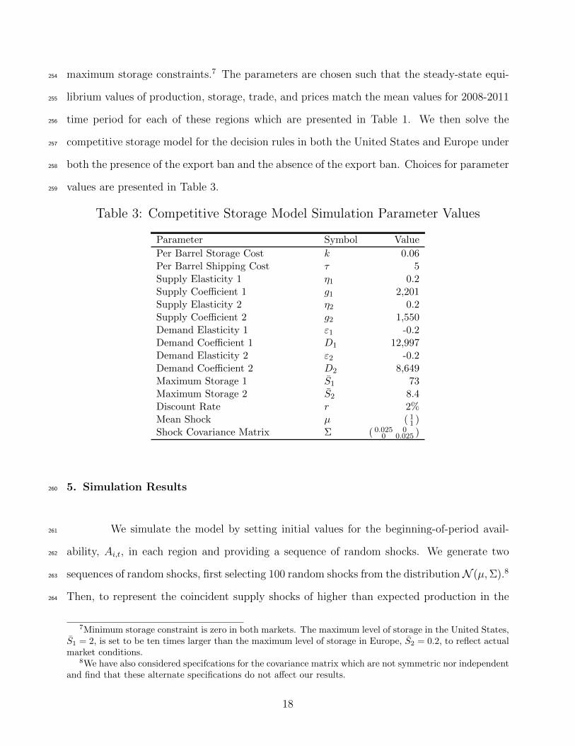
maximum storage constraints.7 The parameters are chosen such that the steady-state equi-254

librium values of production, storage, trade, and prices match the mean values for 2008-2011255

time period for each of these regions which are presented in Table 1. We then solve the256

competitive storage model for the decision rules in both the United States and Europe under257

both the presence of the export ban and the absence of the export ban. Choices for parameter258

values are presented in Table 3.259

Table 3: Competitive Storage Model Simulation Parameter Values

Parameter Symbol Value

Per Barrel Storage Cost k 0.06Per Barrel Shipping Cost τ 5Supply Elasticity 1 η1 0.2Supply Coefficient 1 g1 2,201Supply Elasticity 2 η2 0.2Supply Coefficient 2 g2 1,550Demand Elasticity 1 ε1 -0.2Demand Coefficient 1 D1 12,997Demand Elasticity 2 ε2 -0.2Demand Coefficient 2 D2 8,649Maximum Storage 1 S1 73Maximum Storage 2 S2 8.4Discount Rate r 2%Mean Shock µ ( 1

1 )Shock Covariance Matrix Σ ( 0.025 0

0 0.025 )

5. Simulation Results260

We simulate the model by setting initial values for the beginning-of-period avail-261

ability, Ai,t, in each region and providing a sequence of random shocks. We generate two262

sequences of random shocks, first selecting 100 random shocks from the distributionN (µ,Σ).8263

Then, to represent the coincident supply shocks of higher than expected production in the264

7Minimum storage constraint is zero in both markets. The maximum level of storage in the United States,S1 = 2, is set to be ten times larger than the maximum level of storage in Europe, S2 = 0.2, to reflect actualmarket conditions.

8We have also considered specifcations for the covariance matrix which are not symmetric nor independentand find that these alternate specifications do not affect our results.

18

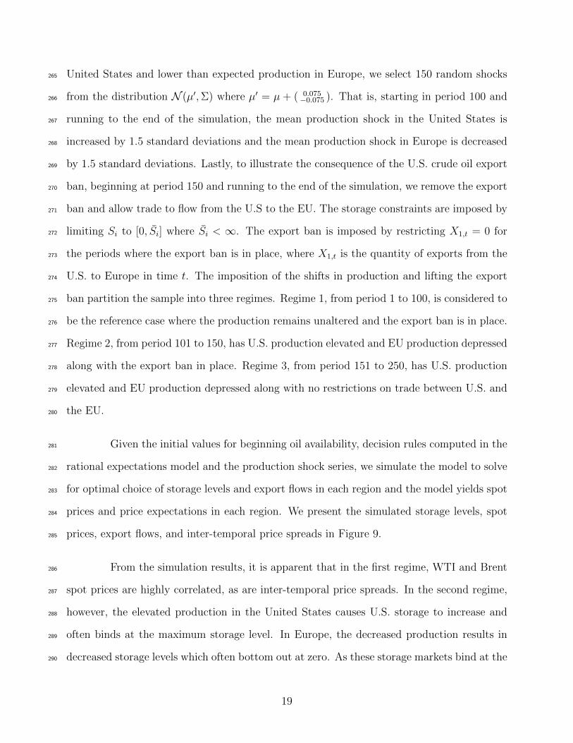
United States and lower than expected production in Europe, we select 150 random shocks265

from the distribution N (µ′,Σ) where µ′ = µ + ( 0.075−0.075 ). That is, starting in period 100 and266

running to the end of the simulation, the mean production shock in the United States is267

increased by 1.5 standard deviations and the mean production shock in Europe is decreased268

by 1.5 standard deviations. Lastly, to illustrate the consequence of the U.S. crude oil export269

ban, beginning at period 150 and running to the end of the simulation, we remove the export270

ban and allow trade to flow from the U.S to the EU. The storage constraints are imposed by271

limiting Si to [0, Si] where Si < ∞. The export ban is imposed by restricting X1,t = 0 for272

the periods where the export ban is in place, where X1,t is the quantity of exports from the273

U.S. to Europe in time t. The imposition of the shifts in production and lifting the export274

ban partition the sample into three regimes. Regime 1, from period 1 to 100, is considered to275

be the reference case where the production remains unaltered and the export ban is in place.276

Regime 2, from period 101 to 150, has U.S. production elevated and EU production depressed277

along with the export ban in place. Regime 3, from period 151 to 250, has U.S. production278

elevated and EU production depressed along with no restrictions on trade between U.S. and279

the EU.280

Given the initial values for beginning oil availability, decision rules computed in the281

rational expectations model and the production shock series, we simulate the model to solve282

for optimal choice of storage levels and export flows in each region and the model yields spot283

prices and price expectations in each region. We present the simulated storage levels, spot284

prices, export flows, and inter-temporal price spreads in Figure 9.285

From the simulation results, it is apparent that in the first regime, WTI and Brent286

spot prices are highly correlated, as are inter-temporal price spreads. In the second regime,287

however, the elevated production in the United States causes U.S. storage to increase and288

often binds at the maximum storage level. In Europe, the decreased production results in289

decreased storage levels which often bottom out at zero. As these storage markets bind at the290

19

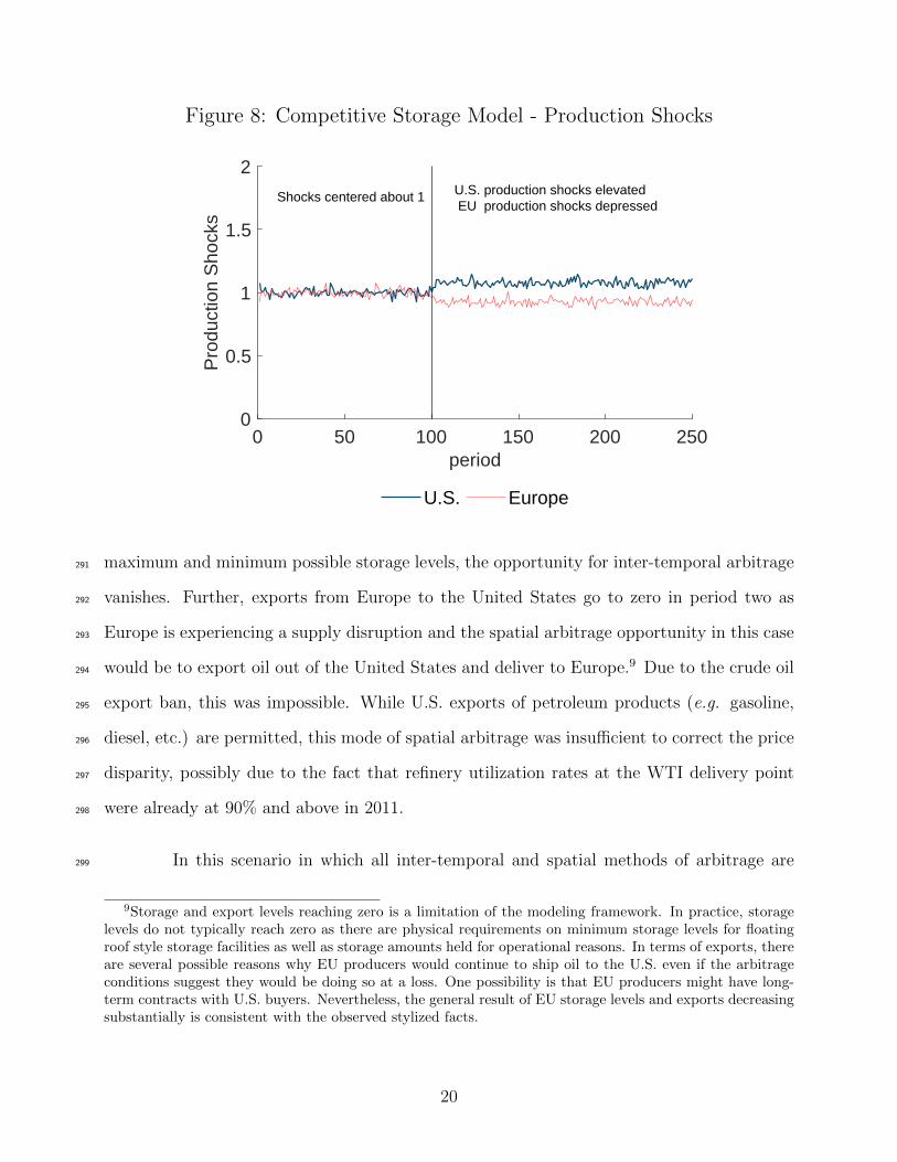
Figure 8: Competitive Storage Model - Production Shocks

0 50 100 150 200 250period

0

0.5

1

1.5

2

Pro

duct

ion

Sho

cks

U.S. Europe

Shocks centered about 1 U.S. production shocks elevated EU production shocks depressed

maximum and minimum possible storage levels, the opportunity for inter-temporal arbitrage291

vanishes. Further, exports from Europe to the United States go to zero in period two as292

Europe is experiencing a supply disruption and the spatial arbitrage opportunity in this case293

would be to export oil out of the United States and deliver to Europe.9 Due to the crude oil294

export ban, this was impossible. While U.S. exports of petroleum products (e.g. gasoline,295

diesel, etc.) are permitted, this mode of spatial arbitrage was insufficient to correct the price296

disparity, possibly due to the fact that refinery utilization rates at the WTI delivery point297

were already at 90% and above in 2011.298

In this scenario in which all inter-temporal and spatial methods of arbitrage are299

9Storage and export levels reaching zero is a limitation of the modeling framework. In practice, storagelevels do not typically reach zero as there are physical requirements on minimum storage levels for floatingroof style storage facilities as well as storage amounts held for operational reasons. In terms of exports, thereare several possible reasons why EU producers would continue to ship oil to the U.S. even if the arbitrageconditions suggest they would be doing so at a loss. One possibility is that EU producers might have long-term contracts with U.S. buyers. Nevertheless, the general result of EU storage levels and exports decreasingsubstantially is consistent with the observed stylized facts.

20

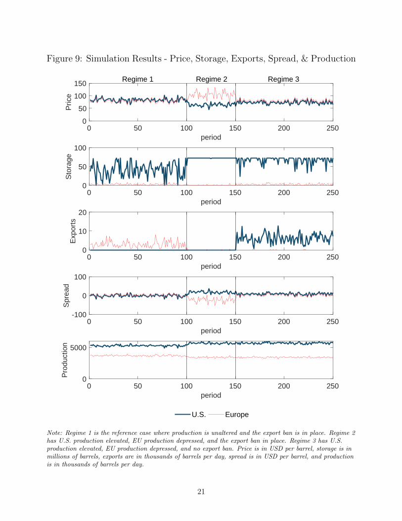
Figure 9: Simulation Results - Price, Storage, Exports, Spread, & Production

0 50 100 150 200 250period

0

50

100

Sto

rage

0 50 100 150 200 250period

0

50

100

150

Pric

e

0 50 100 150 200 250period

0

10

20

Exp

orts

0 50 100 150 200 250period

-100

0

100

Spr

ead

0 50 100 150 200 250period

0

5000

Pro

duct

ion

U.S. Europe

Regime 2Regime 1 Regime 3

Note: Regime 1 is the reference case where production is unaltered and the export ban is in place. Regime 2has U.S. production elevated, EU production depressed, and the export ban in place. Regime 3 has U.S.production elevated, EU production depressed, and no export ban. Price is in USD per barrel, storage is inmillions of barrels, exports are in thousands of barrels per day, spread is in USD per barrel, and productionis in thousands of barrels per day.

21

unavailable, the spot prices of these near identical grades of crude separate. The price in the300

United States falls, the price in Europe rises and the inter-temporal spreads in these regions301

take on opposite shapes. The simulation results replicate the situation where the WTI price302

is lower than Brent, WTI is in contango, Brent is in backwardation, U.S stocks reach the303

maximum, European stocks are drawn down to the minimum, and trade from Europe to the304

U.S goes to zero.305

In the third regime where U.S. production is elevated, EU production depressed,306

and no export ban, the U.S. is able to take advantage of the spatial arbitrage opportunity.307

Following the repeal of the export ban, the simulation indicates oil flowing from the U.S. to308

the EU, storage levels falling in the U.S., storage levels climbing in the EU, and prices and309

price spreads converging back together.310

5.1. Robustness Check311

We consider the scenario where instead of a structural change in supply, we im-312

plement a structural shift in demand. Our original specification implements the structural313

change in supply by shifting the means of the multiplicative supply shocks in Equation 10314

from µ to µ′. In this specification, we leave the mean of the shock distribution constant315

at µ and shift out the EU demand and shift in the U.S. demand, reflecting the change in316

demand due to the reweighting of commodity indices and the increase in Japanese demand.317

Simulating the model under this alternate specification yields equivalent results in terms318

of separation of spot prices, cessation of international trade, hitting storage maximum and319

minimum levels, and yielding opposite price spreads during the period where the structural320

change is implemented and the export ban is in place.321

22

6. Conclusion322

The WTI and Brent contracts compete for the role as the world benchmark price323

of oil. Traders, including hedgers, typically choose one or the other contract. This means324

there is great interest in the WTI-Brent pricing structure, including the shape of the two325

futures curves, the absolute price difference between the two benchmarks, and the dynamics326

of the degree of integration of the markets. These markets are heavily traded (directly327

and indirectly) by hedgers and financial investors. Prices of jet fuel, heating oil, diesel, and328

gasoline follow these markets closely. And there are also a large number of derivative financial329

products such as swaps and options based on either WTI or Brent, or based on the price330

spread between them.331

From early 2011, the price of WTI went to a significant discount to Brent, but332

U.S. crude could not be exported to the world market to arbitrage away the spread. This333

break in the pricing relationship arose largely because of expanded U.S. production, reduced334

production of Brent, and storage capacity factors. For similar reasons, the shape of the two335

futures curves diverged around the same time. WTI was in contango and Brent displayed336

backwardation. We develop a simulation model that explains the change in the pricing337

structure in 2011. The key stylized facts of the WTI and Brent pricing structure are replicated338

with our model. This means the break in the WTI-Brent futures pricing structure can be339

explained by standard commodity storage theory.340

Since the break in the WTI-Brent relationship, a number of fundamental changes341

have occurred in the U.S. crude oil infrastructure. In May 2012, a major pipeline connecting342

the WTI terminal in Cushing, OK to the Gulf Coast reversed it flow direction allowing crude343

to be sent from the WTI terminal to the coast. In December 2015, U.S. Congress lifted344

the crude oil export ban. Given that the barriers to spatial arbitrage in the WTI-Brent345

market have been lifted, the 2011 market segmentation in the crude oil market is unlikely to346

23

reoccur. As a result, the arguments for abandoning WTI as the main crude benchmark have347

been corrected, and the arguments against using Brent as the main global crude benchmark348

remain.349

Acknowledgments350

We appreciate the helpful comments provided by Christopher Thiem at the 2016351

ECOMFIN conference at Essec Business School.352

24

References353

Alquist, Ron, and Justin-Damien Guenette. 2014. “A blessing in disguise: The impli-354

cations of high global oil prices for the North American market.” Energy Policy, 64: 49–57.355

Blas, Javier, and David Blair. 2011. “European crude stocks hit multi-356

year low.” Financial Times. Available at https: // www. ft. com/ content/357

de085f44-f4a8-11e0-a286-00144feab49a .358

BP. 2016. “Sullom Voe Characteristics.” Available at http: // www. bp. com/ en/359

global/ north-sea-infrastructure/ Infrastructure/ Terminals/ Sullom_ Voe/360

Characteristics. html .361

Brennan, Michael J. 1958. “The supply of storage.” The American Economic Review,362

50–72.363

Brown, Stephen PA, and Mine K Yucel. 2013. “The shale gas and tight oil boom:364

Us states’ economic gains and vulnerabilities.” Council on Foreign Relations. Available at365

https: // www. cfr. org/ report/ shale-gas-and-tight-oil-boom .366

Buyuksahin, Bahattin, Thomas K Lee, James T Moser, and Michel A Robe.367

2013. “Physical markets, paper markets and the WTI-Brent spread.” The Energy Journal,368

34(3): 129.369

Chen, Wei, Zhuo Huang, and Yanping Yi. 2015. “Is there a structural change in the370

persistence of WT-Brent oil price spreads in the post-2010 period?” Economic Modelling,371

50: 64–71.372

Deaton, Angus, and Guy Laroque. 1992. “On the behaviour of commodity prices.” The373

Review of Economic Studies, 59(1): 1–23.374

Deaton, Angus, and Guy Laroque. 1996. “Competitive storage and commodity price375

dynamics.” Journal of Political Economy, 896–923.376

25

Dickey, David A., and Wayne A. Fuller. 1979. “Distribution of the estimators for377

autoregressive time series with a unit root.” Journal of the American statistical association,378

74(366a): 427–431.379

Elliott, Graham, Thomas J. Rothenberg, and James H. Stock. 1992. “Efficient tests380

for an autoregressive unit root.”381

Energy Information Administration. 2015. “Crude oil storage at Cushing, but not382

storage capacity utilization rate, at record level.” Available at https: // www. eia. gov/383

todayinenergy/ detail. php? id= 20472 .384

Energy Information Administration. 2016a. “International Energy Statistics.” Available385

at https: // www. eia. gov/ beta/ international/ data/ browser/ .386

Energy Information Administration. 2016b. “New England natural gas pipeline ca-387

pacity increases for the first time since 2010.” Available at https: // www. eia. gov/388

todayinenergy/ detail. php? id= 29032 .389

Energy Information Administration. 2016c. “Petroluem and other liquids data.” Avail-390

able at https: // www. eia. gov/ petroleum/ data. cfm .391

Energy Information Administration. 2016d. “Spot Prices.” Available at https: // www.392

eia. gov/ dnav/ pet/ pet_ pri_ spt_ s1_ d. htm .393

Energy Information Administration. 2016e. “U.S. Crude Oil Imports.” Available394

at http: // www. eia. gov/ dnav/ pet/ pet_ move_ impcus_ a2_ nus_ epc0_ im0_ mbbl_395

m. htm .396

Energy Information Administration. 2016f. “U.S. Field Production of Crude Oil397

Thousand Barrels per Day.” Available at https: // www. eia. gov/ dnav/ pet/ hist/398

LeafHandler. ashx? n= PET& s= MCRFPUS2& f= A .399

26

Energy Information Administration. 2016g. “Weekly Cushing OK Ending Stocks ex-400

cluding SPR of Crude Oil.” Available at https: // www. eia. gov/ dnav/ pet/ hist/401

LeafHandler. ashx? n= PET& s= W_ EPC0_ SAX_ YCUOK_ MBBL& f= W .402

Engle, Robert F, and Clive WJ Granger. 1987. “Co-integration and error correction:403

representation, estimation, and testing.” Econometrica, 251–276.404

Fattouh, Bassam. 2010. “The dynamics of crude oil price differentials.” Energy Economics,405

32(2): 334–342.406

Gardner, Bruce L. 1979. Optimal stockpiling of grain. Lexington Books.407

Gouel, Christophe. 2012. “RECS: Matlab solver for rational expectations models with408

complementarity equations.” Available at https: // github. com/ christophe-gouel/409

recs .410

Gregory, Allan W, and Bruce E Hansen. 1996. “Residual-based tests for cointegration411

in models with regime shifts.” Journal of econometrics, 70(1): 99–126.412

Gustafson, Robert L. 1958. Carryover levels for grains: a method for determining amounts413

that are optimal under specified conditions. Technical Bulletin No. 1178, US Department414

of Agriculture. Available at https: // naldc. nal. usda. gov/ download/ CAT87201112/415

PDF .416

International Energy Agency. 2012. “Oil Market Report Tables - February.” Available417

at https://www.iea.org/media/omrreports/tables/2012-02-10.pdf.418

International Energy Agency. 2016. “Oil Market Report Tables - February.” Available419

at https://www.iea.org/media/omrreports/tables/2016-02-09.pdf.420

Kilian, Lutz. 2016. “The impact of the shale oil revolution on US oil and gasoline prices.”421

Review of Environmental Economics and Policy, 10(2): 185–205.422

27

Makki, Shiva S, Luther G Tweeten, and Mario J Miranda. 1996. “Wheat storage423

and trade in an efficient global market.” American Journal of Agricultural Economics,424

78(4): 879–890.425

Meyer, Gregory. 2011. “Oil traders unravel Cushing mystery.” Financial Times. Available426

at https: // www. ft. com/ content/ ca18995e-f5b1-11e0-be8c-00144feab49a .427

Miranda, Mario J, and Joseph W Glauber. 1995. “Solving stochastic models of com-428

petitive storage and trade by Chebychev collocation methods.” Agricultural and Resource429

Economics Review, 24(1): 70–77.430

Olsen, Knut. 2012. Characterisation and taxation of cross-border pipelines. IBFD.431

Scheid, Brian. 2014. “Could a Jones Act waiver move US crude export policy?” S&P Global432

Platts. Available at http: // blogs. platts. com/ 2014/ 10/ 03/ jones-act-waivers/ .433

The Intercontinental Exchange. 2013. “ICE Brent Crude Oil: Frequently Asked Ques-434

tions.” Available at http: // www. theice. com/ publicdocs/ futures/ ICE_ Brent_435

FAQ. pdf .436

Vidal, John. 2011. “Shell’s failure to protect Nigeria pipeline ‘led to sabotage’.” The437

Guardian. Available at https: // www. theguardian. com/ environment/ 2011/ aug/438

25/ shell-oil-export-nigeria-pipeline-sabotage .439

Wilmoth, Adam. 2012. “Cushing, OK stores more than $4.1 billion in oil.” The Oklahoman.440

Available at http: // newsok. com/ article/ 3660501 .441

Working, Holbrook. 1949. “The theory of price of storage.” The American Economic442

Review, 1254–1262.443

Wright, Brian D, and Jeffrey C Williams. 1982. “The roles of public and private storage444

in managing oil import disruptions.” The Bell Journal of Economics, 341–353.445

28

Ye, Shiyu, and Berna Karali. 2016. “Estimating relative price impact: The case of Brent446

and WTI.”447

29