Score Level versus Audio Level Fusion for Voice Pathology ... · Score Level versus Audio Level...

Score Level versus Audio Level Fusion for VoicePathology Detection on the Saarbrucken Voice

Database

David Martınez, Eduardo Lleida, Alfonso Ortega, and Antonio Miguel

Aragon Institute for Engineering Research (I3A), University of Zaragoza, Spain{david,lleida,ortega,amiguel}@unizar.es

Abstract. The article presents a set of experiments on pathologicalvoice detection over the Saarbrucken Voice Database (SVD). The SVDis freely available online containing a collection of voice recordings ofdifferent pathologies, both functional and organic. It includes recordingsfor more than 2000 speakers in which sustained vowels /a/, /i/, and /u/are pronounced with normal, low, high, and low-high-low intonations.This variety of sounds makes possible to set different experiments, andin this paper a comparison between the performance of a system whereall the vowels and intonations are pooled together to train a single modelper class, and a system where a different model per class is trained foreach vowel and intonation, and the scores of each subsystem are fusedat the end, is conducted. The first approach is what we call audio levelfusion, and the second is what we call score level fusion. For classifica-tion, a generative Gaussian mixture model trained with mel-frequencycepstral coefficients, harmonics-to-noise ratio, normalized noise energyand glottal-to-noise excitation ratio, is used. It is shown that the scorelevel fusion is far more effective than the audio level fusion.

Keywords: Pathological Voice Detection, Saarbrucken Voice Database,GMM, Fusion, MultiFocal toolkit

1 Introduction

The detection of laryngeal pathologies through an automatic voice analysis is one of themost promising tools for speech therapists, mainly due to its noninvasive nature andits objectivity for making decisions. The performance of these systems is neverthelessnot perfect, and nowadays it is used as an additional source of information for otherlaryngoscopial exams [1].

Researchers have focused their efforts on finding new features that could discrim-inate between normal and pathological voices or even assess their quality, but also onfinding different approaches for classification. Some of the most useful features are con-sidered to be acoustic parameters such as mel-frequency cepstral coefficients (MFCC)[17, 1], amplitude and frequency perturbation parameters [9], and noise related parame-ters [2, 6], but there are different alternatives like nonlinear analysis [3, 4]. Regarding tothe classifiers, well-known approaches in speech processing like hidden Markov model

2 D.Martınez, E. Lleida, A. Ortega, A. Miguel

(HMM) [7], Gaussian mixture model (GMM) [1], multilayer perceptron (MLP) [8], orsupport vector machine (SVM) [9], have been studied.

Experiments related with pathological voices can be focused on three main tasks.While the most simple and direct idea is to classify voices as pathological or normal, likein [2, 6, 7, 10, 11], another goal is to assess voice quality according to a perceptual scale,like GRBAS [22, 23], DSI [25, 26] or VPA [24], among others. A third typical problem isto identify a specific pathology, like for example, functional dysphonia in [26], nodulesand other laryngeal injuries in [9], or polyps, keratosis leukoplakia, adductor spasmodicdysphonia and vocal nodules in [5].

The main difficulty when facing a pathological voice related experiment is thedatabase acquisition. Most of the works in the literature make use of the MEEIdatabase, openly commercialized by Kay Elemetrics [12]. But the amount of recordingsis limited and current approaches already give excellent performance, being difficultto evaluate improvements of new ideas. In other cases, private databases collected inlocal hospitals are the alternative. This is costly and generally they are not public.However, recently a new open and freely downloadable database, the SVD [13], hasbeen recorded by the Institute of Phonetics of Saarland University. On it, sustained/a/, /i/ and /u/ vowels, pronounced with normal, low, high and low-high-low into-nations, and a spoken sentence in German, are found, what make of this database avery complete set to conduct experiments, and easy to reach by all the community.In [27] a first approach is conducted to test this database on a pathological voice de-tection task, with GMMs as classifier, MFCC, harmonics-to-noise ratio (HNR) [14],normalized noise energy (NNE) [15], and glottal-to-noise excitation ratio (GNE) [16],as features. Calibration and fusion of scores coming from the subsystems built witheach vowel and intonation is performed with MultiFocal toolkit [18]. MultiFocal toolkitis a toolkit developed by Niko Brummer, and is widely used among the speaker andlanguage recognition community. The fusion results are shown to be very promising.

In this work, following the guidelines marked in [11] to discriminate between normaland pathological voices, a comparison between the fusion techniques used in [27] anda pool-of-data strategy is conducted, where instead of fusing different systems trainedon each vowel and intonation, a single system trained on all vowels and intonationspooled together is used.

The classifier used in this work was also evaluated on MEEI database in [27]. Theresults were close to similar approaches in the bibliography, like [11]. Concretely, theArea Under the Curve (AUC) was 0.943 and 94.93% of pathological files and 95.00%of the normal files were correctly classified.

The rest of the paper is organized as follows: in Section 2, the SVD is presented; inSection 3, the features extracted from the audio are described; in Section 4, the classi-fication, calibration and fusion procedures are explained; in Section 5, the experimentsthat have been performed are presented and analyzed, for the two strategies mentionedabove; and in Section 6, the conclusions of this work are drawn.

2 Saarbrucken Voice Database

This database has been recently made freely available online [13]. It is a collection ofvoice recordings from more than 2000 persons, where a session is defined as a collectionof:

– recordings of vowels /a/, /i/, /u/ produced at normal, high, low and low-high-lowpitch.

Score Level vs. Audio Level Fusion for Voice Pathology Detection 3

– recording of sentence ”Guten Morgen, wie geht es Ihnen?” (”Good morning, howare you?”).

That makes a total of 13 files per session. In addition, the electroglottogram (EGG)signal is also stored for each case in a separate file. The length of the files with sustainedvowels is between 1 and 3 seconds. All recordings are sampled at 50 kHz and theirresolution is 16-bit. 71 different pathologies are contained, including both functionaland organic. For our experiments only files with sustained vowels and people older than18 are used. A total of 1970 sessions are kept, after discarding those where some of therecordings were missing or damaged. 1320 (609 males and 711 females) sessions belongto pathological speakers and 650 (400 males and 250 females) to normal speakers.

3 Features

The features used in this work are divided into two groups, according to their nature:acoustic features, represented by the MFCC, where the aim is to characterize thefrequency content of the signal; and noise related features, represented by HNR, NNEand GNE, where the aim is to measure how good the quality of the signal is, or simply,how noisy it is.

3.1 Acoustic Features

MFCC are a family of parameters widely used for many tasks related with speechprocessing. It makes a frequency analysis of the signal based on the human perceptionof the sounds. This idea matches well with the fact that an experienced speech therapistcan detect the presence of a disorder just by listening to the signal [10].

In the extraction procedure, after downsampling to 25 kHz, a 40 ms window with50% overlap has been used, with a bank of 30 Mel filters, to obtain 15 MFCC pluslog-energy. The first two and last two frames have been discarded to avoid possibleerrors in the edges of the recordings, like peaks due to the on and off switches.

3.2 Noise Related Features

Harmonics-to-Noise Ratio HNR was introduced to measure in an objective man-ner the perceptual feeling of hoarseness in the voice [14]. To calculate it, the signal isfirstly downsampled to 16 kHz, and split into 25 ms length frames, with 10 ms shift.In each frame, a comb filter is applied to the signal to compute the energy in theharmonic components. To the logarithm of this quantity, the log-energy of the noise issubstracted to get the HNR.

Normalized Noise Energy In a similar process to the calculation of the HNR,and also with the signal downsampled to 16 kHz and with 25 ms length frames and 10ms shift, the noise estimation is calculated and normalized by the total energy of thesignal. This was first used in [15] and it assumes that pathological voices are noisierthan normal voices.


Glottal-to-Noise Excitation Ratio The goal of this parameter is to comparethe amount of signal due to vocal folds vibration with the amount of signal due to noiseproduced by air turbulences produced during phonation [16]. It is a good measurementof breathiness, although not the only factor that can cause it. To compute it, the signalis first downsampled to 10 kHz, and frames of 40 ms length with 20 ms shift are taken.For each frame, the spectrum is divided into bands of 2000 Hz with centers separated500 Hz. For each of these bands, the Hilbert envelope in time domain is calculated andthe correlation of this envelope with the envelopes of the bands separated more thanhalf of the bandwidth (in this case, bands must be at least 1000 Hz) is computed. TheGNE is the maximum of all correlations. For a normal voice, the correlation should behigh, because all bands should be excited at the same time when the glottis is closed.

4 Classification, Calibration and Fusion

4.1 Classification

The features extracted from the signal are used to train a generative GMM [21] foreach class. For D-dimension features x calculated in a frame-by-frame basis, a GMMprobability density function has the form

p(x|ω, µ,Σ) =

K∑k=1

ωkN (x|µk, Σk), (1)

where K is the number of Gaussians in the model, ωk is the weight of the kth Gaussian,and N (x|µk, Σk) is the Gaussian function with mean µk and covariance Σk.

For each test file y, the likelihoods for pathological and normal classes are calcu-lated, calibrated as explained in section 4.2, and the log-likelihood ratio between themis obtained as

LLK(y) = log p(y|pathological)− log p(y|normal), (2)

which will decide to which class the file belongs.

The metrics to evaluate the performance used in this work are the AUC of the re-ceiver operating characteristic (ROC), the equal-error-rate (EER), the detection costfunction (DCF) or empirical Bayes risk, and its minimum value for the selected oper-ating point (minDCF) [18]. DCF is defined as

DCF = πCmissPmiss + (1− π)CfaPfa, (3)

for a false alarm cost Cfa, a miss cost Cmiss, a prior probability for the target class π, afalse alarm probability Pfa, and a miss probability Pmiss. DCF is a calibration-sensitivemetric, since it depends on the current threshold. However, minDCF is calibration-insensitive, and it gives the minimum cost that could have been obtained with optimalcalibration, at every operating point. It is calculated by varying the threshold from −∞to∞ for each operating point, and then picking the minimum. AUC and EER are alsocalibration-insensitive metrics. We are interested in the hard decisions made by ourclassifier to decide if a voice is pathological or not, therefore we find more interestingto use calibration sensitive metrics like DCF. AUC and EER can be useful in earlystages of our system development, when hard decisions are not of immediate interestand we are only interested in the goodness of uncalibrated scores [19].


4.2 Calibration and Fusion

MultiFocal toolkit [18] is used for calibration and fusion. This toolkit developed inMatlab is primarily designed for calibrating and fusing scores of a language recognitiontask. The goal of the toolkit is twofold: i) to calibrate scores so cost effective Bayesdecisions can be made, by setting the threshold to the Bayes decision threshold, η,

η = logCfa

Cmiss− logit(π), (4)

being the pathological voices our target class; and ii) to fuse scores coming from dif-ferent recognizers to obtain a better recognizer. In our experiments, Cfa = Cmiss = 1,π0 = π1 = 0.5, and threshold equal to the Bayes decision threshold, in our case η=0.

The idea behind calibration is that our scores are converted in such a way that theBayes decision threshold can be used for making the best possible decisions. Equiva-lently, the user could tune the threshold manually to minimize the error metric.

To calculate calibrated log-likelihoods, l′(xt), MultiFocal optimizes another calibration-sensitive metric, Cllr, through a discriminative logistic regression, and obtains a scalarα, and a vector β [20]. Then

l′(xt) = αl(xt) + β, (5)

where l(xt) is the uncalibrated log-likelihood obtained from the classifier.More generally, to fuse K systems what we want is our calibrated log-likelihoods

to be a linear combination of the uncalibrated log-likelihoods of the K systems,

l′(xt) =

K∑k=1

αklk(xt) + β. (6)

As we can check, the fusion is a generalization of the calibration of a single system(K=1), and since the fusion is also a calibration, due to the linearity of the operation,there is no need to pre-calibrate each input system, or to post-calibrate the fusion [18].

5 Experiments

The experiments conducted in this work are divided in two, according to the strategyfollowed to combine all the different varieties of sounds. The first strategy is the oneimplemented in [27], where an individual subsystem is trained for each vowel andintonation, and a discriminative score level fusion of all the subsystems is performedwith MultiFocal toolkit. We will revise this experiment in the first part of section 5.1.In the second part of this section, an experiment has been configured with a singlecommon GMM trained with all the files of all vowels and intonations, and the fusionis made with the scores tested over this common model. This will make possible to seeif the different sounds are correlated and we can take benefit from one to the other.The second strategy trains a unique model per class by concatenating all the files withthe different sounds belonging to the same speaker, and in the test phase, all the filesbelonging to the same speaker are also concatenated and tested over this model as asingle file. This is called audio level fusion.

The features used as input for our classifiers will be 19-dimensional, including 15MFCC + log-energy + HNR + NNE + GNE, all of them mean and variance normalizedwithin each file. A 30-fold strategy is followed in all experiments, in which for every testfold, the remaining 29 are used for training. Then, an average performance measure isextracted from the 30, in the same manner as in [11].


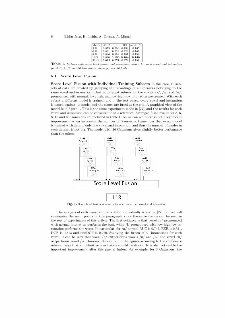
Metric AUC EER DCF minDCF3 G 0.879 0.206 0.198 0.1656 G 0.891 0.226 0.228 0.1698 G 0.886 0.191 0.187 0.15816G 0.890 0.190 0.184 0.14836 G 0.899 0.274 0.274 0.191

Table 1. Metrics with score level fusion and individual models for each vowel and intonation

for 3, 6, 8, 16 and 36 Gaussians. Average over 30 folds.

5.1 Score Level Fusion

Score Level Fusion with Individual Training Subsets In this case, 12 sub-sets of data are created by grouping the recordings of all speakers belonging to thesame vowel and intonation. That is, different subsets for the vowels /a/, /i/, and /u/,pronounced with normal, low, high, and low-high-low intonation are created. With eachsubset a different model is trained, and in the test phase, every vowel and intonationis tested against its model and the scores are fused at the end. A graphical view of themodel is in figure 1. This is the same experiment made in [27], and the results for eachvowel and intonation can be consulted in this reference. Averaged fused results for 3, 6,8, 16 and 36 Gaussians are included in table 1. As we can see, there is not a significantimprovement when increasing the number of Gaussians. Remember that every modelis trained with data of only one vowel and intonation, and thus the number of modes ineach dataset is not big. The model with 16 Gaussians gives slightly better perfomancethan the others.

Fig. 1. Score level fusion scheme with one model per vowel and intonation

The analysis of each vowel and intonation individually is also in [27], but we willsummarise the main points in this paragraph, since the same trends can be seen inthe rest of experiments of this article. The first evidence is that vowel /a/ pronouncedwith normal intonation performs the best, while /i/ pronounced with low-high-low in-tonation performs the worst. In particular, for /a/ normal AUC is 0.747, EER is 0.321,DCF is 0.313 and minDCF is 0.270. Studying the fusion of all intonations for eachvowel, it can be seen that vowel /a/ outperforms vowels /u/ and /i/, and vowel /u/outperforms vowel /i/. However, the overlap in the figures according to the confidenceinterval, says that no definitive conclusions should be drawn. It is also noticeable theimportant improvement after this partial fusion. For example, for 3 Gaussians, the


relative improvement in AUC is 7.63%, and in DCF is 12.78%, comparing /a/ withall pronountiations fused and /a/ normal. If we look at the intonations, the variabilityis high: among the results with /a/, the normal intonation works better, for /i/ thelow intonation works better, and for /u/ the low-high-low intonation is the one thatperforms the best. As we see, no specific intonation is better than others, and it de-pends on the vowel pronounced by the subject. With the global fusion with all vowelsand intonations a huge increase in performance is obtained. Comparing with the bestresult without fusion (/a/ normal), the increase in perfomance, again for the case of 3Gaussians, is 17.67% for the AUC and 36.74% for the DCF. We believe that the mainreason is the fact of having much more data, and containing different information,because they come from different vowels and intonations. Note that these results areoptimal in terms of the fusion, since the fusion parameters have been trained on thetest data. If we compare this fusion with the partial fusion of each vowel, it can be seenthat all vowels contribute to the improvement, because the global fusion outperformsthe partial ones.

Fig. 2. Score level fusion scheme with a common model for all vowels and intonations

Score Level Fusion with a Common Training Subset This experiment issimilar to the one in the previous section, where a late fusion with MultiFocal toolkitis done, but training a common GMM with all training data, including all vowels andintonations. Then, in the test phase, every vowel and intonation is tested against thiscommon model and the scores are fused at the end. The scheme can be seen in figure2. In table 2 averaged results are shown for the metrics described in Section 4.1. Onlyfusion results are shown for 3, 6, 8, 16 and 36 Gaussians. In this case, as the modelincludes all the sounds, it could be expected to reach a higher number of Gaussiansrobustly trained. However, as it can be seen in the tables, the best results are obtainedwith 16 Gaussians. The individual behavior of the different vowels and intonations issimilar to the previous case, being the best results obtained for /a/ pronounced withnormal intonation.

More interesting is the comparison with the results of the previous experiment.Comparing tables 1 and 2, in both experiments the optimal number of Gaussians is16, and the differences between each other are not meaningful. In short, we obtain nobenefit when training the models with all data, mixing all vowels and intonations. That



Table 2. Metrics with score level fusion and a common model for all vowels and intonations

for 3, 6, 8, 16 and 36 Gaussians. Average over 30 folds.

can be a sign of being each of the sounds really independent of each other, becausethey do not take advantage of a bigger model trained with the pool of the data.

5.2 Audio Level Fusion

In this case, we train a single GMM with data coming from all vowels and pronoun-ciations, as in the second experiment of section 5.1. In the test phase, all the filesbelonging to the same speaker are concatenated and evaluated as just one single file.The difference with the previous case is that now a single score per speaker is obtainedand no score level fusion is needed. A graphical scheme can be seen in figure 3. In table3 we have the averaged results in terms of AUC, EER, DCF and minDCF for 3, 6, 8,16 and 36 Gaussians. For comparison with the first case of section 5.1 (also in [27]),note that there we needed 12 (models) × [3 (Gaussians per model) × [19 (means) +190 (Σ)]+3 (weights)] + 12 (fusion weights) + 2 (fusion offsets) = 7574 parametersfor 3 Gaussians, and 90734 parameters for 36 Gaussians. Now, in the most demandingcase, the one with 36 components, we need 36 (weights) + 36 × [ 19 (means) + 190(Σ) ] + 1 (calibration weight) + 2 (calibration offset) = 7563 parameters. We see thatthe audio level fusion makes possible to save parameters, since the most demandingcase is similar to the least demanding case of the score level fusion. The interest liesin checking if it is better an early fusion, as the one presented in this section, or a latefusion, as the one presented in the previous subsection.

Fig. 3. Audio level fusion scheme

As it can be checked in the different experiments, the performance is much betterwhen fusing at score level that when concatenating the different files of the samesession and doing the test of a single file. For example, with 16 Gaussians, the relativeimprovement of using score level fusion with individual training subsets for each vowel



Table 3. Audio level fusion metrics for 3, 6, 8, 16 and 36 Gaussians. Average over 30 folds.

and intonation with respect to the audio level fusion is 12.94% in terms of AUC and35.21% in terms of DCF. Since the number of parameters is very similar between thecase of score level fusion with a 3 component GMM and the case of audio level fusionwith 36 component GMM, more similar results could be expected. One explanationcould be that the audio level fusion is more sensitive to errors in any of the concatenatedfiles, whereas in the score level fusion, the fact of having different weights for each ofthe sounds makes the system more flexible and able to give stronger weights to thesounds working better.

As in section 5.1, the fact of having longer files with larger sound variability couldtake benefit of a model with more components. But also in this case it can be appreci-ated that the 16 Gaussian model gives slightly better results than the rest, supportingthe theory presented before, stating that every vowel and intonation is independent ofthe rest and there is no benefit of a bigger model trained with all sounds. Note alsothat the audio level fusion gives improvements with regard to the case where only oneof the vowels and intonations is considered.

6 Conclusions

SVD is an open and free database available online. The amount of recordings of differentsounds and intonations contained in this database makes possible to conduct differentand interesting experiments. In this article a comparison between voice pathology de-tection experiments carried out on the SVD with a score level fusion and an audio levelfusion is presented. The score level fusion refers to the process in which every file witha different vowel and intonation is tested separately and the scores are fused at theend. The audio level fusion refers to the concatenation of the files with different soundsinto a single file that is evaluated to obtain directly a single likelihood. A robust GMM,trained on MFCC, log-energy and HNR, NNE and GNE, has been used as classifier.The score level fusion gives better results than the audio level fusion. For a modeltrained with 16 Gaussians, the AUC is a 12.94% higher and DCF a 35.21% lower inthe former than in the latter. The improvement of the score level fusion results withrespect to the evaluation of a single vowel and intonation alone is also huge: a 17.67% inAUC and 36.75% in DCF, with respect to /a/ pronounced in normal intonation, whichis the one with the best individual performance. It is also interesting to see that theoptimal number of Gaussians is 16 both in the score level and in the audio level fusion.In addition, training a bigger model with the different sounds pooled into the same filegives no further benefit, an indication of independence among different sounds.

7 Acknowledgements

This work was funded by the Spanish Ministry of Science and Innovation under projectsTIN2011-28169-C05-02 and INNPACTO IPT-2011-1696-390000.


References

[1] J. I. Godino Llorente, et al.. “Dimensionality Reduction of a Pathological Voice Quality Assess-ment System Based on Gaussian Mixture Models and Short-Term Cepstral Parameters”, IEEETr. Biomed. Eng. 53, no. 10, 2006.

[2] N. Saenz-Lechon, et al., “Methodological Issues in the Development of Automatic Systems forVoice Pathology Detection”, Biomed. Signal Proc. and Control 1, no. 2, 2006.

[3] J.J. Jiang and Y. Zhang, “Nonlinear Dynamic Analysis of Speech from Pathological Subjects”,Electron. Lett. 38, no. 6, 2002.

[4] Y. Zhang and J.J. Jiang, “Nonlinear Dynamic Analysis in Signals Typing of Pathological HumanVoices”, Electron. Lett. 39, no. 13, 2003.

[5] M. Markaki and Y. Stylianou, “Using Modulation Spectra for Voice Pathology Detection andClassification”, Proc. IEEE EMBS Annual Intern. Conf., Minneapolis, MN, 2009.

[6] V. Parsa and D.G. Jamieson, “ Identification of Pathological Voices Using Glottal Noise Mea-sures”, J. Speech, Lang. and Hearing Res. 43 (2), 2000.

[7] L. Gavidia-Ceballos and J. H. L. Hansen, “Direct Speech Feature Estimation Using an IterativeEM Algorithm for Vocal Fold Pathology Detection”, IEEE Tr. Biomed. Eng. 43, no. 4, 1996.

[8] R. Tadeusiewicz, et al., “The Evaluation of Speech Deformation Treated for Larynx Cancer UsingNeural Network and Pattern Recognition Methods”, Proc. EANN 1998.

[9] A. Gelzinis, et al., “Automated Speech Analysis Applied to Laryngeal Disease Categorization”,Comput. Methods Programs Biomed. 91, 2008.

[10] J. D. Arias-Londono, et al., “On Combining Information from Modulation Spectra and Mel-Frequency Cepstral Coefficients for Automatic Detection of Pathological Voices”, Logop. Phoni-atrics Vocology, 2010.

[11] N. Saenz Lechon, “Contribuciones Metodologicas para la Evaluacion Objetiva de Patologıas

Larıngeas a partir del Analisis Acustico de la Voz en Diferentes Escenarios de Produccion”, PhDThesis, 2010.

[12] Kay Elemetrics Corp., “Disordered Voice Database”, Version 1.03 [CD-ROM], October 1994,MEEI, Voice and Speech Lab, Boston, MA.

[13] W. J. Barry and M. Putzer, “Saarbrucken Voice Database”, Institute of Phonetics, Univ. ofSaarland, http://www.stimmdatenbank.coli.uni-saarland.de/.

[14] E. Yumoto, et al., “Harmonics-To-Noise Ratio as an Index of the Degree of Hoarseness”, J.Acoust. Soc. Am. 71, 1982.

[15] H. Kasuya, et al., “Normalized Noise Energy as an Acoustic Measure to Evaluate PathologicVoice”, J. Acoust. Soc. Am. 80, no. 5, 1986.

[16] D. Michaelis, et al., “Glottal-to-Noise Excitation Ratio. A New Measure for Describing Patho-logical Voices”, Acustica/Acta acustica 83, 1997.

[17] S. B. Davis and P. Mermelstein, “Comparison of Parametric Representations for MonosyllabicWord Recognition in Continuously Spoken Sentences”, IEEE Tr. Acoust. 28, no. 4, 1980.

[18] N. Brummer, “FoCal Multi-class: Toolkit for Evaluation, Fusion and Cal-ibration of Multi-class Recognition Scores - Tutorial and User Manual”,http://sites.google.com/site/nikobrummer/focalmulticlass.

[19] N. Brummer, “The BOSARIS ToolkitUser Guide: Theory, Algorithms and Code for BinaryClassifier Score Processing”, http://sites.google.com/site/bosaristoolkit.

[20] N. Brummer and J. A. du Preez, “ Application-Independent Evaluation of Speaker Detection”,Computer Speech and Language 20, no. 2-3, 2006.

[21] D. A. Reynolds and R. C. Rose, “Robust Text-Independent Speaker Identification Using Gaus-sian Mixture Models”, IEEE Tr. on Speech and Audio Proc. 3, 1995.

[22] M. Hirano, “Clinical Examination of Voice”, Springer Verlag, New York, 1981.[23] N. Saenz-Lechon, et al., “Automatic Assessment of Voice Quality According to the GRBAS

scale”, Proc. 28th IEEE EMBS Annual Intern. Conf., 2006.[24] P. Carding, et al., “Formal Perceptual Evaluation of Voice Quality in the United Kingdom”,

Logop. Phoniatrics Vocology 25, 2000.[25] F. Wuyts, et al., “The Dysphonia Severity Index: An Objective Measure of Vocal Quality Based

on a Multiparameter Approach”, J. Speech, Lang. and Hearing Res. 43, 2000.[26] M. M. Hakkesteegt, et al., “The Relationship between Perceptual Evaluation and Objective

Multiparametric Evaluation of Dysphonia Severity”, J. of Voice 22, 2008.[27] D. Martınez, et al., “ Voice Pathology Detection on the Saarbrucken Voice Database with

Calilbration and Fusion of Scores Using MultiFocal Toolkit”, submitted to Iberspeech 2012,Madrid.

Score Level versus Audio Level Fusion for Voice Pathology ... · Score Level versus Audio Level...

Documents

Transcript of Score Level versus Audio Level Fusion for Voice Pathology ... · Score Level versus Audio Level...