Scoping Profitable CO2 Projects in Wyoming

Prepared byOwen R. Phillips,

Klaas T. van ’t Veldand

Benjamin R. Cook Department of Economics and Finance and

Enhanced Oil Recovery InstituteUniversity of Wyoming

July 22, 2009

2

Overview Review EORI CO2 scoping model.Provide detail on project costs.Update estimated demand for CO2 and incremental oil production for economic field reservoir combinations. Update estimated cumulative demand for CO2 in a basin and for the State of Wyoming.Provide the economics for a specific field-reservoir combination.

3

4

5

There are four “screening” steps for identifying profitable EOR projects.

Broadly, these steps are described as follows:

6

Identify “promising” fields

Fields with > 5 MMBO cumulative oil production

Gas to oil ratio < 3,000 or API < 50

Screen for miscibility

Estimate MMP

Miscible flood if MMP < fracture pressure

Estimate CO2-EOR response

Scaled analog approach

Screen for profitability

7

Data Needed for ScopingFor each field-reservoir

Distance to proposed trunk lineOOIPAreaDepthAPITemperatureFracture gradientFormation volume factors (oil and CO2)Number of wells (producing, injection, temporarily abandoned)Current oil production rateCurrent water production rateOil decline rateAverage water flood injection rate (reservoir thickness and permeability)

8

Establish MMP for each reservoirMeasured MMP Estimate based on API and temperature

Calculate fracture pressureFracture gradient from Wyoming O&G Conservation Commission

9

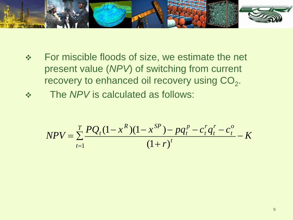
For miscible floods of size, we estimate the net present value (NPV) of switching from current recovery to enhanced oil recovery using CO2.

The NPV is calculated as follows:

NPV = PQt (1− x R )(1− xSP )− pqtp − ct

rqtr − ct

o

(1+ r)tt=1

T∑ −K

10

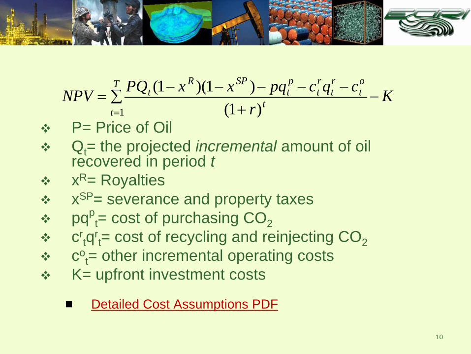
P= Price of OilQt= the projected incremental amount of oil recovered in period txR= RoyaltiesxSP= severance and property taxespqp

t= cost of purchasing CO2cr

tqrt= cost of recycling and reinjecting CO2

cot= other incremental operating costs

K= upfront investment costs

Detailed Cost Assumptions PDF

NPV = PQt (1− x R )(1− xSP )− pqtp − ct

rqtr − ct

o

(1+ r)tt=1

T∑ −K

11

Implementing the above estimation of NPV requires estimates of a field-reservoir combination's (FRC’s) “response” to EOR. FRC responses are the projected time paths of incremental oil recovery, CO2purchases, and CO2 recycling.

12

We use an "analog” approach based ondimensionless curves to predict the response of an oil field to EOR..

13

The Analog Approach

Step 1: Estimate baseline oil production at the existing, analog EOR project and the new, candidate EOR project.Step 2: Convert the quantities of CO2 and water injected and of CO2 and incremental oil produced over time at the analog project into fractions of that project’s HCPV. Step 3: Plot the time series for cumulative incremental oil production and cumulative CO2production against the injection time series.

14

Step 4: Assume that future injection and production at the candidate project, when converted into fractions of that project’s hydrocarbon pore volume (HCPV), will follow the analog dimensionless curves Step 5: Convert estimated injectivity at the candidate project to fractions of its HCPV per unit time Step 6: Determine predicted incremental oil recovery and CO2 production rates at the candidate project, expressed in fractions of its HCPV per unit time Step 7: Convert the predicted production rates into units relevant to the economic analysis

15

0.2 0.4 0.6 0.8 1.0 1.2 1.4 1.6 1.8 2.00-0.02

0

0.02

0.04

0.06

0.08

0.10

0.12

0.14

0.16

CO2 + Water Injection (HCPV)

Lost Soldier Tensleep

Wertz Tensleep

West Texas San Andres

16

Results of analysisThe following tables and figures highlight some the results of our analysis

We set oil price= $70 a barrel and CO2= $2.00/mcf. We assume a required return of 20% and a well spacing of 80 acres/well.We use the Lost Soldier Ten Sleep (LSTP) dimensionless curves as our analogs.

17

18

19

20

21

22

In Summary :Oil Price $70, CO2 Price $2.00, ROR 20%, 80 Acre Well Spacing, and LSTP Analog

Cum CO2 Demand Additional Oil(bcf) (mmbo)

Powder River Basin (30) 392.5 61.1Wind River Basin (20) 466.5 71.4Big Horn Basin (40) 1,485.7 192.9Green River Basin (19) 335.4 92.8TOTAL (109) 2,680.1 418.2

23

Grieve-Muddy (Wind River Basin) Selected Reservoir Parameters

Characteristic Assumed ValueOriginal Oil in Place (OOIP) 87 Million

Cumulative Oil Production 32.04 Million(37% of OOIP)

Well Bores (all TA’d) 28

Average Depth 6,790 feet

Fracture Pressure 4,068 psi

Initial Pressure 2,950 psi

Minimum Miscibility Pressure 1,676 psi

Oil Gravity -37º API

Average Porosity 20%

Average Permeability 220 md

24

Characteristic ValueActive Producing Wells 0

Active Injection Wells 0

Number of TA'd Wells 28

Injectors Required 14

Producers Required 14

New Wells to Drill 0

Water Injection Rate (bbls/well/month) 43,751

Maximum Gas Production (MMCFD) 10

Recycling Horsepower Required 1,097

Grieve-Muddy (Wind River Basin)Selected Cost Considerations

25

Capital Cost Items (K) $ Millions

Inactive Producer Well Conversions (14) $ 4.58

Producer Well Surface Equipment $ 0.45

Injector Well Conversions (14) $ 2.41

Injection Well Surface Equipment $ 0.70

Cost of Recycling Equipment $ 1.32

Total Startup Capital Investment $ 9.45*

Grieve-Muddy (Wind River Basin)

•These capital costs DO NOT include the cost of the CO2 transport pipeline and metering station.

•3-mile spur pipeline and metering station is estimated to add an additional $990,000 which would bring the total initial capital investment to $10.45 Million.

26

Grieve-Muddy (Wind River Basin) Baseline Scoping Results

Analog Oil Price

CO2 Price

($/mcf)

Cum. CO2

Demand(Bcf)

Operating Period

Avg. CO2 Demand

First 4 Years(MMcfd)

Avg. CO2 Demand

Last Years(MMcfd)

PV of Profits ($MM)

Inc. Oil Prod.

(Mmbo)

LSTP $70 $2.00 30.8 28 yrs 7.3 2.4 $67.3 6.8

KMSA $70 $2.00 40.8 40 yrs 15.8 1.4 $87.7 14.9

Disclaimer Results from the scoping model contain data estimates, and assume the recovery features of the analog being used. Detailed field models and simulations should be conducted before CO2 projects are initiated.

27

Estimated Costs for the SpurCost of Pipeline: $840,000Cost of Meter Station: $150,000

Total: $990,000

28

LSTP Inc. Recovery:6.8 MMBO (28 yrs)

KMSA Inc. Recovery: 14.9 MMBO (40 yrs)

29

•Assume Lost Soldier Tensleep Analog

Discounted Net Profits: $67.3 Million

30

Daily CO2 Injection Rate:11.2 MMCFD

Total Incremental Recovery: 6.8 MMBO

•Assume Lost Soldier Tensleep Analog