A Presentation

Gautam Babbar 11CHardik Parmar 14CUtkarsh Modi 52CAmitabh Anand 4C

 

Kumar Anubhav 19CDebleena Banerjee 23KSahil Jain 50K

 

Supply Chain Management Demand Forecast for HiTek Computers

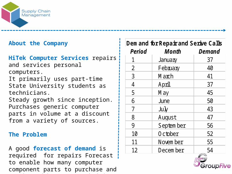
About the Company

HiTek Computer Services repairs and services personal computers.It primarily uses part-time State University students as technicians. Steady growth since inception.Purchases generic computer parts in volume at a discount from a variety of sources.

The Problem

A good forecast of demand is required  for repairs Forecast to enable how many computer component parts to purchase and stock, and how many technicians to hire.

Demand for Repair and Serive CallsPeriod Month Demand1 January 372 February 403 March 414 April 375 May 456 June 507 July 438 August 479 September 5610 October 5211 November 5512 December 54

The Approach

We are to use Exponential Smoothing Method for the Forecasts as mentioned in the problem.

Data of past 12 months considered.

The Smoothing constants considered are i) Alpha = 0.3ii) Alpha = 0.5

Calculations performed in OM Tools(Refer attached Excel)

The Solution

To develop the series of forecasts for the data in this table, we will start with period 1 (January)and compute the forecast for period 2 (February) using  α= 0.30. The formula for exponential smoothing  also  requires  a  forecast  for  period  1, which  we  do  not  have, so  we  will  use  the demand for period 1 as both demand and forecast for period 1Thus, the forecast for February is 37 service calls=(0.30)(37) +(0.70)(37)

The forecast for period 3 is computed similarly:

F3 =aD2 +(1 -a)F2=37.9 service calls

Exponential Smoothing Method

The Solution (continued)

The Final forecast isfor Period 13, January, and is the forecast of interest to HiTek:

=F13 =αD12 +(1 -α)F12

=(0.30)(54) +(0.70)(50.84)

51.79 service calls

(with Smoothing Constant α = 0.30)

Period Demand Forecast1 37 37.002 40 37.003 41 37.904 37 38.835 45 38.286 50 40.307 43 43.218 47 43.159 56 44.3010 52 47.8111 55 49.0712 54 50.8513 51.79

Exponential Smoothing Method

The Solution (continued)

The Final forecast isfor Period 13, January, and is the forecast of interest to HiTek:

=F13 =αD12 +(1 - α)F12

=(0.50)(54) +(0.50)(53.21)

53.61 service calls

(with Smoothing Constant α= 0.50)

Period Demand Forecast1 37 37.002 40 37.003 41 38.504 37 39.755 45 38.386 50 41.697 43 45.848 47 44.429 56 45.7110 52 50.8611 55 51.4312 54 53.2113 53.61

Exponential Smoothing Method

1 2 3 4 5 6 7 8 9 10 11 12

0

10

20

30

40

50

60

Period

Demand

Forecast

1 2 3 4 5 6 7 8 9 10 11 12

0

10

20

30

40

50

60

Period

Demand

Forecast

Alpha = 0.30 Alpha = 0.50

Please refer to the calculations on OM Tool here OM Tools Calculation

Exponential Smoothing Method

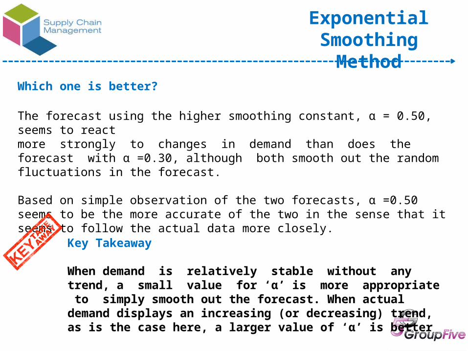
Which one is better?

The forecast using the higher smoothing constant, α = 0.50, seems to reactmore  strongly  to  changes  in  demand  than  does  the  forecast  with α =0.30, although  both smooth out the random fluctuations in the forecast.

Based on simple observation of the two forecasts, α =0.50 seems to be the more accurate of the two in the sense that it seems to follow the actual data more closely.

Key Takeaway

When demand is relatively stable without any trend, a small value for ‘α’ is more appropriate to simply smooth out the forecast. When actual demand displays an increasing (or decreasing) trend, as is the case here, a larger value of ‘α’ is better

Exponential Smoothing Method

The ApproachWe are to use Trend Adjusted Exponential Smoothing Method for the Forecasts as mentioned in the problem.Data of past 12 months considered.

The Smoothing constants considered are i) Alpha = 0.3ii) Alpha = 0.5

Trend Adjustment Constants considered arei. Beta = 0.3ii. Beta = 0.5Calculations performed in OM Tools(Refer attached Excel)

The Solution

To develop the series of forecasts for the data in this table, we will start with period 1 (January)and compute the forecast for period 2 (February) using α = 0.30 and β=0.30 The formula for trend adjusted exponential smoothing  also  requires  a  forecast  for  period  1, which  we  do  not  have, so  we  will  use  the demand for period 1 as both demand and forecast for period 1 & T(t+1) {trend} as 0 for periods 1 & 2Thus:F₂ = 0.30 * 37.00 + (1-0.30)*(37.00+0.00) = 37.00T ₂= 0.00 , FIT ₂ = F ₂ + T ₂ = 37.00

F₃ = 0.30 * 40.00 + (1-0.30)*(37.00+0.00) = 37.90T ₃= 0.30 * (37.90 – 37.00) + (1-0.30)*(0.00) = 0.27FIT ₃ = F ₃ + T ₃ = 37.90 + 0.27 = 38.17

Ft = a(At - 1) + (1 - a)(Ft - 1 + Tt - 1)Tt = b(Ft - Ft - 1) + (1 - b)Tt - 1

Step 1: Compute Ft

Step 2: Compute Tt

Step 3: Calculate the forecast FITt = Ft + Tt

Exponential Smoothing with Trend Adjustment

The Solution (continued)

The Final forecast isfor Period 13, January, and is the forecast of interest to HiTek:

F₁₃ = 0.30 * 54 + (1-0.30) * (48.43 + 1.36)       = 49.15T ₁₃ = 0.30 * (49.15-48.43) + (1-0.30)*1.36       = 1.17FIT ₁₃ = F ₁₃ + T ₁₃ = 50.32

50.32 service calls

(with Smoothing Constant α = 0.30)(with Trend Adjustment Factor β = 0.30)

Exponential Smoothing with Trend Adjustment

The Solution (continued)

The Final forecast isfor Period 13, January, and is the forecast of interest to HiTek:

F₁₃ = 0.50 * 54 + (1-0.50) * (51.53 + 1.73)       = 51.90T ₁₃ = 0.50 * (51.90-51.53) + (1-0.50)*1.73       = 1.05FIT ₁₃ = F ₁₃ + T ₁₃ = 52.95

52.95 service calls

(with Smoothing Constant α = 0.50)(with Trend Adjustment Factor β = 0.50)

Exponential Smoothing with Trend Adjustment

α = 0.30 β = 0.30

Please refer to the calculations on OM Tool here OM Tools Calculation

α = 0.50 β = 0.50

1 2 3 4 5 6 7 8 9 10 11 120

10

20

30

40

50

60

Actual Demand Forecasted Demand

1 2 3 4 5 6 7 8 9 10 11 120

10

20

30

40

50

60

Demand Forecasted Demand

Exponential Smoothing with Trend Adjustment

Trend Projections

Fitting a trend line to historical data points to project into the medium to long-range

Least Squares Method

Linear trends can be found using the least squares technique

y = a + b*x^

where y = computed value of the variable to be predicted (dependent variable)a = y-axis interceptb = slope of the regression linex = the independent variable

^ Equations to calculate the regression variables

b =Sxy - nxy

Sx2 - nx2

y = a + b*x^

a = y – b*x

Least Squares Method

Period(x) Demand(y) X² XY1 37 1 372 40 4 803 41 9 1234 37 16 1485 45 25 2256 50 36 3007 43 49 3018 47 64 3769 56 81 50410 52 100 52011 55 121 60512 54 144 648

∑X =78 ∑Y= 557 ∑X² =650 ∑XY = 3867X = 6.5 Y = 46.42

TotalAverage

b =Sxy - nxy

Sx2 - nx2= 1.723 a = y – b*x = 35.24

Least Squares Method

The trend line is y = 35.24 + 1.72x

1 2 3 4 5 6 7 8 9 10 11 120

10

20

30

40

50

60

Demand(y) Forecast

Please refer to the calculations on OM Tool here OM Tools Calculation

Error Calculation

Mean Absolute Deviation (MAD)

MAD = ∑ |Actual - Forecast|

n

Mean Squared Error (MSE)

MSE =∑ (Forecast Errors)2

N-1

Mean Error (ME)

ME = ∑ Actual - Forecast

n

Mean Absolute Percentage Deviation(MAPD)

MAPD = ∑ |Actual - Forecast|

∑ Actual Demand

Mean Absolute Percent Error (MAPE)

MAPE =∑100|Actuali - Forecasti|/Actuali

n

i=1

n

Please refer to the calculations on OM Tool here OM Tools Calculation

Method Comparison

METHODS/ERROR TYPES

Exponential Smoothing (α = 0.30)

Exponential Smoothing (α = 0.50)

Trend Adjusted

Exponential Smoothing (α = 0.30 &

β =0.30)

Trend Adjusted

Exponential Smoothing (α = 0.50 &

β =0.50)

Least Squares Method

MAD 18.64 12.63 24.03 16.71 2.28MAPD 0.40 0.27 0.52 0.36 0.05

∑E -120.94 -73.97 -165.43 -106.70 -0.04ME -5.26 -3.22 -7.19 -4.64 0.00

MSE 512.23 372.97 585.67 409.33 9.46MAPE 9.05% 7.75% 10.59% 8.79% 4.97%

Method with least amount of error metrics should be preferred for forecasting purposes

*