Chapter 2

GEOSTATISTICAL ANALYSIS OF DOLLAR SPOT EPIDEMICS IN MICHIGAN

IntroductionDollar spot disease of turfgrasses is caused by the pathogen, Sclerotinia

-homoeocarpa F.T. Bennett (2). The disease is common throughout the world and

is destructive to both cool and warm season grasses (18, 19, 21). In North

America, with the exception of the Pacific Northwest, dollar spot is the most

important pathogen of most cultivated fine turfgrass species (18, 21). In

Michigan, the disease is a major.problem for most golf courses where the

epidemic begins in June and can continue into late September. The disease can

blight large areas of turf as a result of coalescing disease foci and can cause

extensive damage if left untreated. Diseased turf impairs the playing surface by

creating depressions that affect ball roll and areas of bare soil where weed

species can encroach on the area (18, 21).

The biology of dollar spot has not been studied extensively due to the

relative ease with which this disease can be controlled with fungicides. Outside of

Great Britain, dollar spot has not been reported to form sexual or asexual spores

(1, 13, 18, 19). Hsiang and Mahuku (11) reported that a population from Ontario

exhibited DNA fingerprints that were consistent with sexual reproduction, but no

fruiting bodies or spores were found. Nitrogen fertility is an important, factor in the

management of dollar spot (4, 14, 18, 19, 21, 25). Most reports support the view

that increased fertility leads to a reduction in the severity of the disease (14, 18,

19, 21, 25). However, Couch and Bloom (4) reported that the susceptibility of

24

Poa pratensis was actually increased in higher fertility treatments in the

greenhouse, but that the effect would be masked in the field because symptoms

would not appear before the rapidly growing, infected leaf blades were mown off.

Spread of the disease is widely believed to be the result of direct movement of

the pathogen on infected blades during mowing operations, and human transport

of infected clippings on shoes, balls, etc. (7, 18, 19,21,25).

Little or no research exists on inoculum sources, but some reports

contend that stromatized infected tissue is the primary inoculum source for the

pathogen (7, 25). Control of dollar spot via fungicide application is generally

accomplished using the contact fungicide, chlorothalonil. However, the EPA has

recently banned the use of this fungicide on home lawns, and future restrictions

on commercial use of chlorothalonil is expected. Because the amount of

fungicide available to an individual golf course is expected to be limited, it will

become critical for superintendents to be able to apply chlorothalonil judiciously

in areas that require treatment. Other fungicides are available for control, but

fungicide resistant dollar spot populations have been reported for most of them

including, the demethylation inhibiting (DMI) (8), benzimidazole (5, 23), and

dicarboximide (5) fungicides.

Studying the epidemiology of a plant disease traditionally calls for the

assessment of the severity or occurrence of disease over some area of interest.

These data are generally collected over an area using some sampling scheme.

However, traditional statistical techniques require adherence to assumptions

such as the independence of samples and normality of data. It makes intuitive

25

sense that plants located closer in space to a diseased plant have a higher

probability of becoming infected than plants located farther away. Recently, using

the location of these samples in space as an additional datum has led to the

description of disease epidemics over space and time using geostatistical

techniques (20, 24, 26, 27).

Important epidemiological questions arise from spatially explicit

descriptions of disease: Is the disease appearance clustered in space? If so,

what factors contribute to this clustering? What practices might ameliorate the

effects of those factors? Can we predict both when and where disease is going to

occur so that fungicide applications can be targeted? One method available to

address these questions is geostatistics. Originally developed for the study of

geological phenomena, geostatistics have found wide application in a number of

fields including phytopathology (20, 24, 26, 27). The primary goal of these

techniques is to explain how a variate of interest (e.g. disease severity) at a

location in space is correlated with all the other points where the variate has

been measured (9, 10, 12, 15, 17). Further treatments allow for the prediction of

the variate at unmeasured locations, and the assessment of prediction

confidence. These techniques also allow for the analysis of nominal values such

as genotypes or size classes in a similar manner (9, 10). Geostatistics provides a

powerful set of tools that can yield insight into the dynamic nature of plant

disease.

Research in plant disease epidemiology using geostatistical tools is

relatively new. Geostatistics have been used to study the spatial pattern of

26

disease incidence and severity (20, 26) and inoculum levels (24, 27). These tools

have also been used to study physico-chemical properties of soils (10), plant

distributions and ecology (15, 17), and microbial distributions (20, 26, 27).

Variography was used by Wollum and Cassel (26) to study the spatial variability

of Rhizobium japonicum in soil planted with soybeans. They concluded that

geostatistics were a good tool for studying the dynamics of microbial populations.

Stein et. al. (20) examined the spatia-temporal development of Peronospora

parasitica epidemics in cabbage (Brassica oleracea). They were able to

determine that spatial variability of the fields was dependent on disease

incidence. They also found spatial dependence when fields were recovering from

disease. Xiao et. al. (27) studied the spatial patterns of Verticillium dahliae

microsclerotia in the soil, and verticillium wilt in cauliflower using geostatistics.

They found that the spatial structure of microsclerotia in the soil was not very

strong. The structure of the microsclerotia did not playa role in the clustered

appearance of disease. They attributed this to a very high amount and fairly

uniform distribution of microsclerotia. They concluded other factors affect the

appearance of wilt. However, they did find that the severity of the wilt was

associated positively with the weak spatial pattern for the presence of

microsclerotia. The information generated by a geostatistical approach to the

study of plant disease epidemics allows obg/~ develop or refine management\... ~

strategies, and help to determine the contributing factors that deserve further

study. Ultimately, this information can be used to design models that can be used

27

to predict the occurrence of plant disease, helping to minimize pesticide

applications, or make cultural practices more effective.

We had 3 objectives: 1) to observe dollar spot epidemics and determine if

disease occurrence has a spatial structure, 2) if a spatial structure is present,

determine the geostatistical parameters associated with the spatial structuring, 3)

Determine if the spatial structure changes during an epidemic, or over seasons.

Materials and Methods

Samplirg. the study site was established at the Robert HancockI

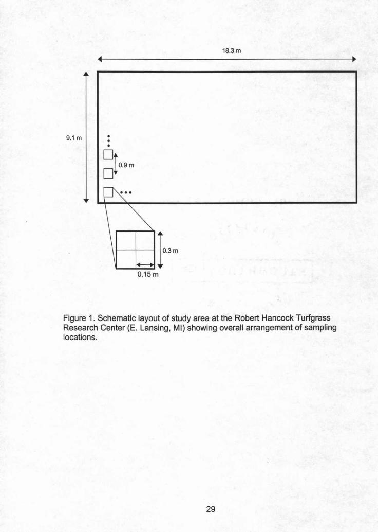
Turfgrass Research Center on a 9.1 m X 18.3 m area of creeping bentgrass

(Agrostis palustris Huds.) and annual bluegrass (Poa annua L.). The study site

received no fungicide applications from 2000-2002. The study site was divided

into 200 0.3 m2 areas on a regular grid at 0.9 m intervals in 2000. In 2001, 23

additional 0.30 m2 areas were established at random locations within the study

site, and all 223 areas were subdivided into four 0.15 m subareas (Fig. 1). These

additional locations were added and all areas subdivided to increase the number

of data pairs at small lag distances. Each subarea's x,y coordinates were

recorded using its center. A 0.3 m2 wooden frame that was divided into quadrants

was used to delineate the subareas. Two points at each sampling location were

marked with marking paint in order to place the frame at the same location at

each sample time. Isolates were also collected from an arbitrarily selected dollar

spot at each location in July 2000 and the vegetative compatibility group (VCG)

for each iSolate was determined in order to assess if clustering was present in

VCGs (Appendix 1).

28

9.1 m

18.3m

•c, •

•

O.15m

Figure 1. Schematic layout of study area at the Robert Hancock TurfgrassResearch Center (E. Lansing, MI) showing overall arrangement of samplinglocations.

29

Data Collection. Dollar spot foci were counted three times per week in

2000 and twice per week in 2001 and 2002 from each of the locations in the

study area. Foci were counted when they reached a size large enough to

observe. This helped to minimize the possibility of accidentally counting an area

that was not a true dollar spot. Counting of the study area was stopped in each

year when disease became prevalent enough in a location that there were too

many disease foci to count accurately.

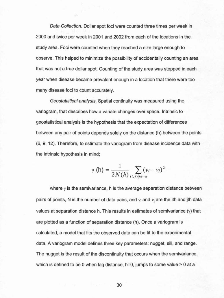
Geostatistical analysis. Spatial continuity was measured using the

variogram, that describes how a variate changes over space. Intrinsic to

geostatistical analysis is the hypothesis that the expectation of differences

between any pair of points depends solely on the distance (h) between the points

(6,9, 12). Therefore, to estimate the variogram from disease incidence data with

the intrinsic hypothesis in mind;

y (h) = 1 L (Vi - Vj) 2

2N(h) (i,j)lhij=h

where y is the semivariance, h is the average separation distance between

pairs of points, N is the number of data pairs, and Vi and vj are the ith and jth data

values at separation distance h. This results in estimates of semivariance (y) that

are plotted as a function of separation distance (h). Once a variogram is

calculated, a model that fits the observed data can be fit to the experimental

data. A variogram model defines three key parameters: nugget, sill, and range.

The nugget is the result of the discontinuity that occurs when the semivariance,

which is defined to be 0 when lag distance, h=O, jumps to some value> 0 at a

30

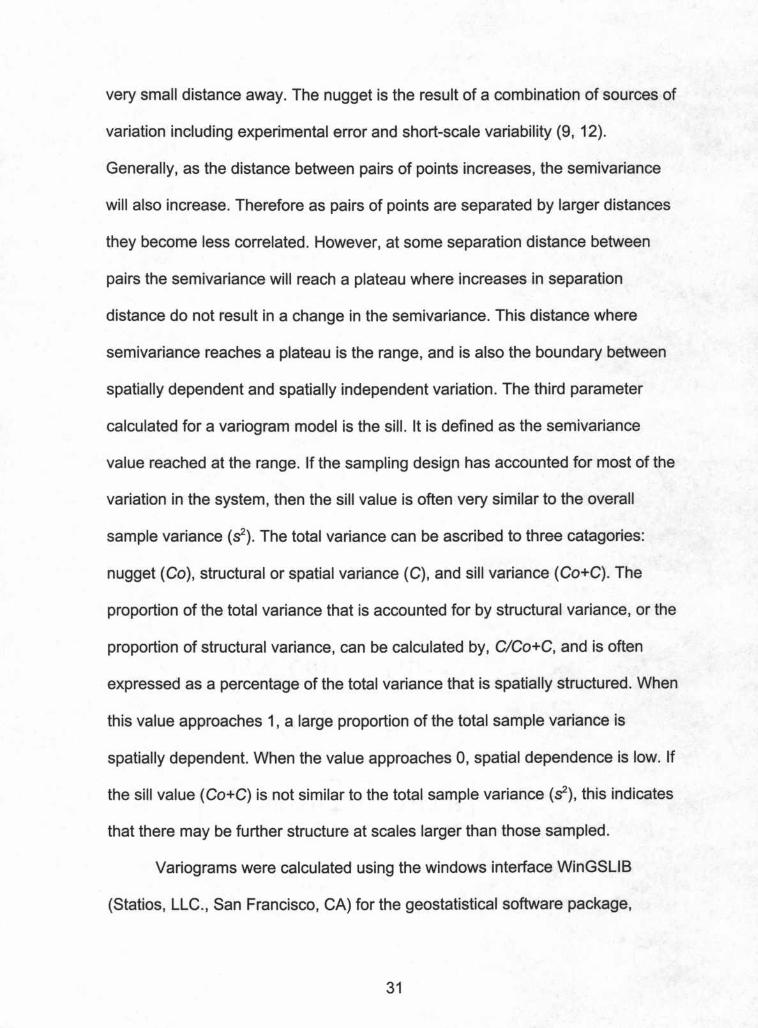
very small distance away. The nugget is the result of a combination of sources of

variation including experimental error and short-scale variability (9, 12).

Generally, as the distance between pairs of points increases, the semivariance

will also increase. Therefore as pairs of points are separated by larger distances

they become less correlated. However, at some separation distance between

pairs the semivariance will reach a plateau where increases in separation

distance do not result in a change in the semivariance. This distance where

semivariance reaches a plateau is the range, and is also the boundary between

spatially dependent and spatially independent variation. The third parameter

calculated for a variogram model is the sill. It is defined as the semivariance

value reached at the range. If the sampling design has accounted for most of the

variation in the system, then the sill value is often very similar to the overall

sample variance (S2). The total variance can be ascribed to three catagories:

nugget (Co), structural or spatial variance (C), and sill variance (Co+C). The

proportion of the total variance that is accounted for by structural variance, or the

proportion of structural variance, can be calculated by, C/Co+C, and is often

expressed as a percentage of the total variance that is spatially structured. When

this value approaches 1, a large proportion of the total sample variance is

spatially dependent. When the value approaches 0, spatial dependence is low. If

the sill value (Co+C) is not similar to the total sample variance (S2), this indicates

that there may be further structure at scales larger than those sampled.

Variograms were calculated using the windows interface WinGSLIB

(Statios, LLC., San Francisco, CA) for the geostatistical software package,

31

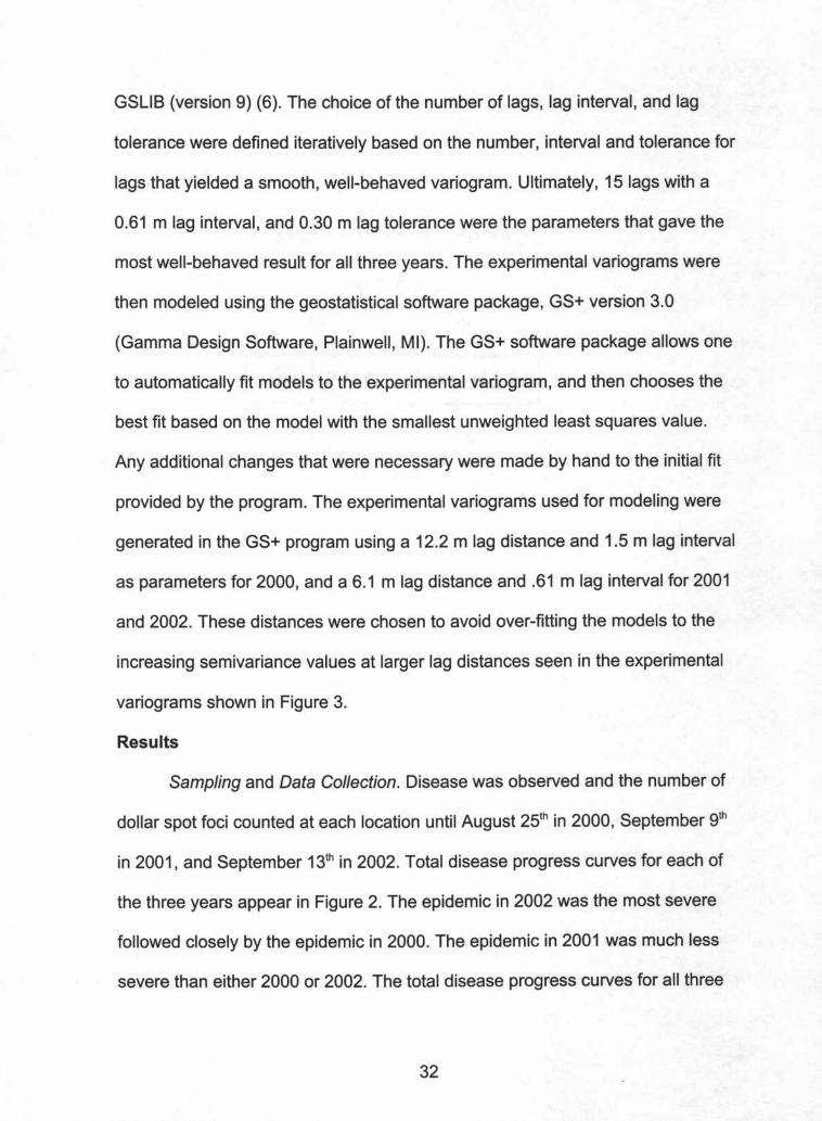
GSLIB (version 9) (6). The choice of the number of lags, lag interval, and lag

tolerance were defined iteratively based on the number, interval and tolerance for

lags that yielded a smooth, well-behaved variogram. Ultimately, 15 lags with a

0.61 m lag interval, and 0.30 m lag tolerance were the parameters that gave the

most well-behaved result for all three years. The experimental variograms were

then modeled using the geostatistical software package, GS+ version 3.0

(Gamma Design Software, Plainwell, MI). The GS+ software package allows one

to automatically fit models to the experimental variogram, and then chooses the

best fit based on the model with the smallest unweighted least squares value.

Any additional changes that were necessary were made by hand to the initial fit

provided by the program. The experimental variograms used for modeling were

generated in the GS+ program using a 12.2 m lag distance and 1.5 m lag interval

as parameters for 2000, and a 6.1 m lag distance and .61 m lag interval for 2001

and 2002. These distances were chosen to avoid over-fitting the models to the

increasing semivariance values at larger lag distances seen in the experimental

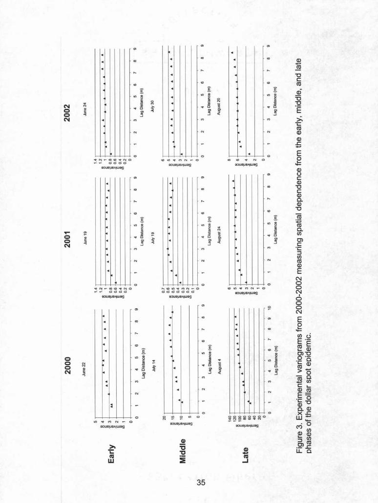
variograms shown in Figure 3.

Results

Sampling and Data Collection. Disease was observed and the number of

dollar spot foci counted at each location until August 25th in 2000, September 9th

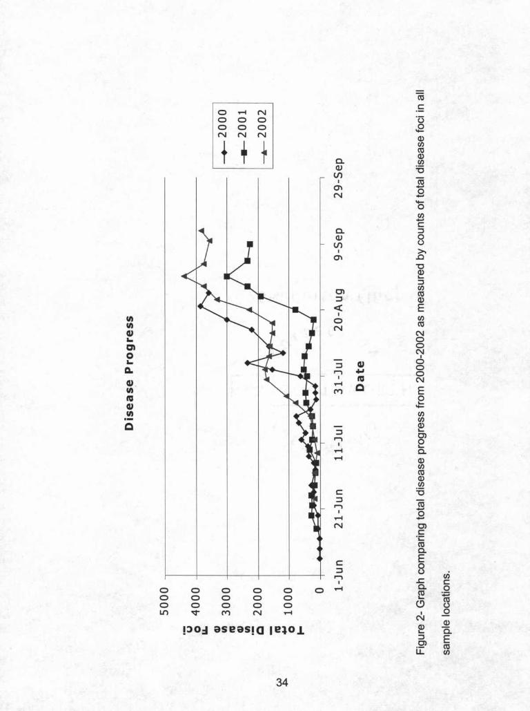
in 2001, and September 13th in 2002. Total disease progress curves for each of

the three years appear in Figure 2. The epidemic in 2002 was the most severe

followed closely by the epidemic in 2000. The epidemic in 2001 was much less

severe than either 2000 or 2002. The total disease progress curves for all three

32

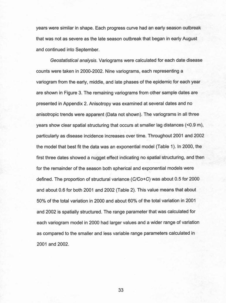
years were similar in shape. Each progress curve had an early season outbreak

that was not as severe as the late season outbreak that began in early August

and continued into September.

Geostatistical analysis. Variograms were calculated for each date disease

counts were taken in 2000-2002. Nine variograms, each representing a

variogram from the early, middle, and late phases of the epidemic for each year

are shown in Figure 3. The remaining variograms from other sample dates are

presented in Appendix 2. Anisotropy was examined at several dates and no

anisotropic trends were apparent (Data not shown). The variograms in all three

years show clear spatial structuring that occurs at smaller lag distances «0.9 m),

particularly as disease incidence increases over time. Throughout 2001 and 2002

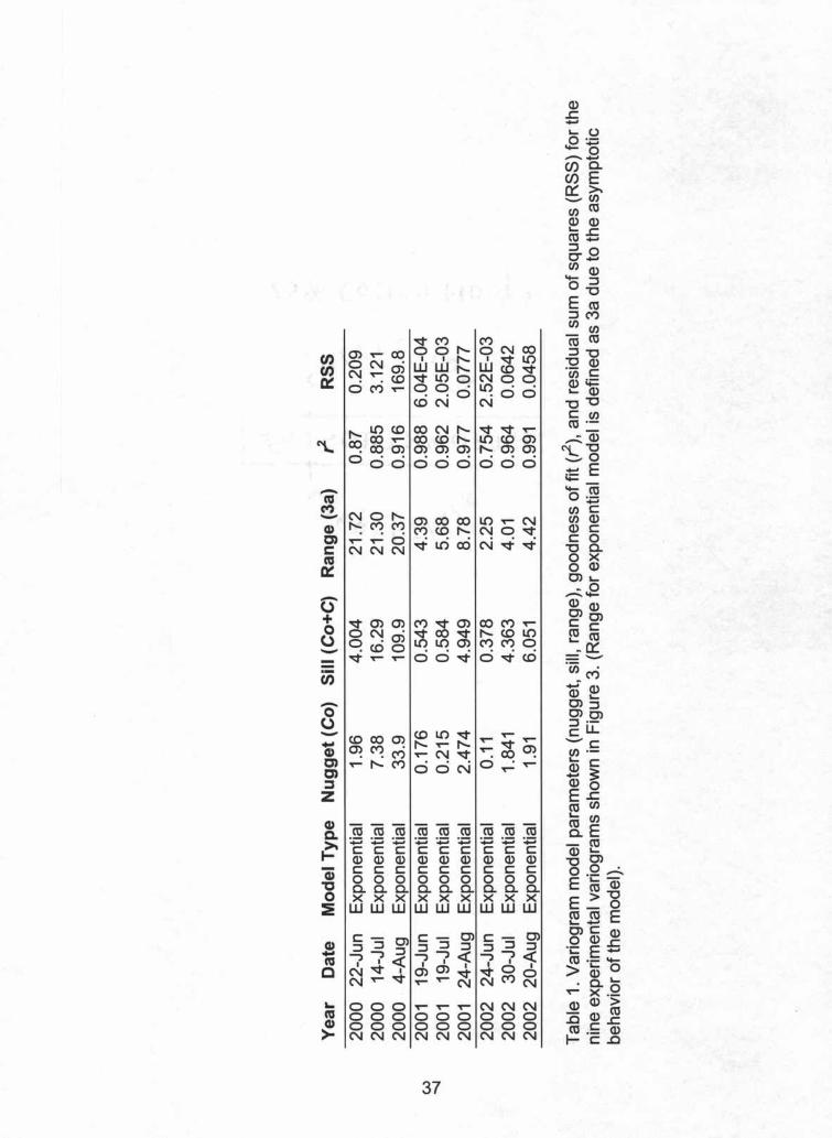
the model that best fit the data was an exponential model (Table 1). In 2000, the

first three dates showed a nugget effect indicating no spatial structuring, and then

for the remainder of the season both spherical and exponential models were

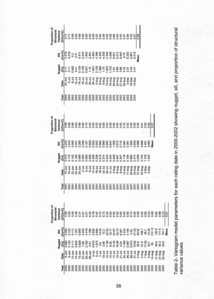
defined. The proportion of structural variance (C/Co+C) was about 0.5 for 2000

and about 0.6 for both 2001 and 2002 (Table 2). This value means that about

500/0of the total variation in 2000 and about 60%) of the total variation in 2001

and 2002 is spatially structured. The range parameter that was calculated for

each variogram model in 2000 had larger values and a wider range of variation

as compared to the smaller and less variable range parameters calculated in

2001 and 2002.

33

coc

0 '1""'"4 N0 0 0 °00 0 0 ~N N N Q)

f T 1 encoc. Q)

o~Q) "'C(J)

I coen •...0N •...

'+-0en•...c

C. :::JQ) 0(J) U

I ~en .o"'CQ)L-

:::JCl enco::J Q)

« EI enU) 0

U) N cocu Ni.. 0m 0

N0 Ii.. ::J cu 0D. 0r"""\ •••• 0

I to Ncu '1""'"4 QU) M Eto 0cu L-'+-U) enenQ Q)

::J L-

0>r"""\ 0I L-'1""'"4 C.'1""'"4

Q)encoQ)en

c :.c::J cor"""\ •...I 0'1""'"4 •...

N 0>C

°Ccoc.c E

0::J Ur"""\ .c en

I c0 0 0 0 0 0 '1""'"4 C. 0co +:i0 0 0 0 0 L- eo0 0 0 0 0 (9 oLf') ~ M N '1""'"4 I 0

N Q)

!:>0:l aseas!o le~o~ Q) c.L-

:::J E0>u:: coen

34

'tN~CO<O'tNO ""<OIt)'t"'N~O.. 0000 0000000a:lUepe,,1lUas aouepe"llUas

0)0)

..• ..• CO..• CO

..•..•

,... ..•..• ..• <0

..•(0 ~..•

..• I It) e0 It) Q) ~ e

~ oc: ~ ~ ~ 't0 N ~ S u;0 N VI >. 't Cl ::J

Q) "<t is ~ ..• Cl Cl

N c: co ::J::J ..• 01 ..J «-, III ..•..J

..• '" ..•..•

..• N

..•

..•

..•

..•

..•

•

..•

~I«

~

NooN

'tN~CO<O'tNO.. 0000aouepe,,!was

~ooN

..•

..•

•4

•4

•..•

•~••• ~

~

<0

~It) Q)

oc 0CO N]j u;

't c ::JCl ClCO ::J

..J -c

'"N

•o o<01t)'t"'N 0

aoue!Je,,!was

<0

~sc~ ~

't 0 >.Cl ~CO..J

N

..•

••••~~•4

•• •

..•

0)

•CO

,...4

C(0

I c

Q)o 'tC N

.~ u;'t Cl ::J

Cl 4Cl ~CO..J

'" ~..•

N •

o o

N

•.~

•0

0 0 ~ ~ It) 0N

It) "<t '" N .•.. 0 aOUepe"!Wasaouepe"!Was

~ ~"C

't: :ECOw :E

35

0)

..•

•••~ <0

~It) Q)

oe~

't 0Clco..J

'"

4 N

••..•

t---+--+--t----+ 0

co <0 't N 0

aOUepe"!Was

•

t--r-+--+---+---+-+ 0

<01t)'t"'N~OaOUepe"!Was

••..••..•

••

••~

..•~

00000000~~~CO{o,"¢N

CJ)•..CO..J

<0

IIt) Q)

(,J

C

~'t 0

Clco..J

'"

N

<0 ~Q)(,J

CIt) ~

0't

Clco..J

'"

0'.•...0)

"'0c:0)

0'"'0"'0·E~

"'i::::0)0'0'..c.•...Ee'+-0'oc:0'"'0c:0'0.

0'"'0

0)+:i0)0.en0>c:

·C::Jen0)0'ENooN

IoooNE£en UE·-0) EL- 0'0> "'00·-._ 0L- 0'0) .•..•> 0-0lYenc: L-

0' 0)E._005"'00.0'X..cW:::·0

('t)en

0' CDL- en::J 0).2> ..c

u..O

Proportion of Structural Variance

0.900.800.700.60ob 0.50

~ 0.40o0.300.200.100.00 -t------,------,--------,----.---,---------,

150

- -e- 2000D 2001

-.*-·2002

170 250 270190 210 230Day of Year (base 365)

I

f

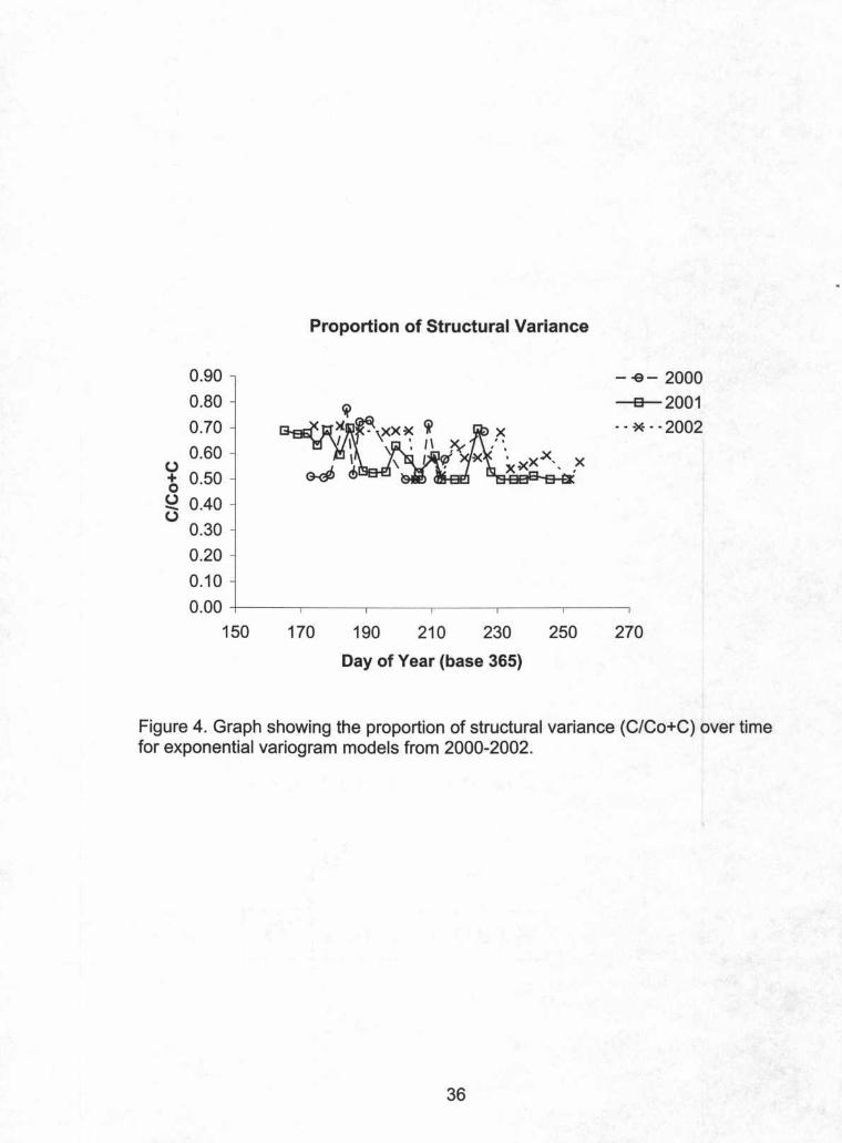
Figure 4. Graph showing the proportion of structural variance (C/Co+C) over timefor exponential variogram models from 2000-2002.

36

-ns('I)-Q)C)ens

~

co co co co co co co co co+:i+:i+:i+:i+:i+:i+:i+:i+:iC C C C C C C C CID ID ID ID ID ID ID ID IDC C C C C C C C C00000 0 0000.0.0.0.0.0.0.0.0.X X X X X X X X XWWWWWWWWW

37

IDs:-"- ()O+:i'+-0--wo.wE0:::>'_ enen COID IDro=::J 00"_en ID'+-::J0"CE co::JC'?en enco co::J"C"CID

'00 CIDt+="- ID"C"CC enco·-~ID"l."C_0~Eo.~-en Cen IDID CC 0"Co.o Xo ID0>,,-- 0-'+-ID ID0>0>

C CCO CO"-- 0:::=-'00 cot)~IDID "-O>::J0>0>ELi:-cen'-"- C2~ID 0E.c.co en"- en~E-coID "-"co>O.Q~E ro IDE>"C

_0~ 19 EO>CIDOID.c.'C E -CO .- '+->"-0ID "-.0.0~ x.-ID ID >-IDCO.cc.c.CO._ ID~c.c

~~~~~~~~~~~~~~~~~~~~~~~ooooooooooooooooooooo~NNNNNNNNNNNNNNNNNNNNN

.•....0 0 t--LOLOLOLO0000

NN(t)(J)~CON.•....LOCO LOCO CO CO t--LO00000000

38

~::J

""-'U::JL..

""-'Cf)\f-oCoto0-

e0-

"0

Cro

..;CD0>0>::JC0>C.§o.cCf)

NooN

IoooNC

CD""-'ro

"0

0>C~~.coroCDL..

~~CD

""-'CDE~ro0-

CD"0

oEE~ .0>Cf)o CD·C ::Jro ro»I CDNU

CD ffi.0 ·Cro roI- >

Discussion

Although the total disease severity during the epidemics in each of the

three years was different, there were also several similarities between the

epidemics. First, the disease progress curves were similar in shape (Fig. 2). All

three progress curves showed that dollar spot first appears in early to mid June

with a minor outbreak and then becomes much more severe during the months

of August and September. Our data agree with those of other researchers that

have shown the later season phase of the epidemic is most damaging to a turf

area (7, 16, 18, 21). Disease progress was similar in each year despite

differences in disease severity indicating that environmental parameters playa

large role in the overall severity and timing of dollar spot outbreaks. In all three

years dollar spot was observed to decrease in presence during July, presumably

because of the hot, humid growing conditions present during that time. These

results support the view that environmental parameters are primarily responsible

for disease appearance and resulting overall severity.

The experimental variograms that were calculated for each date were also

similar over time. Once a variogram is calculated for each date in the study, a

model is calculated that fits the observed data. One reason to fit models to the

data is so that the key model parameters the nugget, range, and sill, can be

compared to observe how they change over time. The sampling design

determines the smallest scale at which spatial relationships can be resolved. In

2000 the design consisted of 2000.3 m2 areas spaced on 0.9 m centers. The

limitations of this design is that the smallest lag interval for the calculated

39

variogram was 0.9 m, and there was no information about the disease at smaller

scales. If spatial dependence exists at a scale smaller than the smallest sampled

interval, then it would become a part of the nugget variance and would not be

accounted for in the variogram. In 2000, the calculated variograms displayed

spatial dependence, and about 50% of the total variation was spatially structured

(Table 2). In 2001 and 2002 23 additional areas were added randomly to the

study site, and the 0.3 m2 areas were subdivided into four 0.15 m2 subareas to

protect against the possible problem of the scale of spatial dependence.

Increasing the resolution of the sampling design increased the information about

small-scale variability. As the smallest sampling interval was 0.15 m, the addition

of the random locations was important to be able to evaluate lag distances

between 0.15 m and 0.9 m. These changes in the sampling design resulted in a

gain of information as reflected by a 100/0increase in the proportion of structural

variance from 500/0in 2000 to 60% in 2001 and 2002 (Table 2). This increase in

spatial resolution at the smaller scales is why there is a much stronger spatial

dependence observed for the 2001 and 2002 data as compared to the 2000

data. Based on the experimental variograms calculated for all three years we

conclude that dollar spot incidence is spatially correlated in our study area, and

that the spatial correlation is present on a small scale. Other locations should be

included in future studies to determine if dollar spot incidence at other locations is

similarly spatially correlated.

Interestingly, the nugget and sill values for variogram models from each

date scale with one another indicating that the spatial structure is relatively stable

40

over time. The stability of this relationship can also be seen in the stability of the

proportion of structural variance (C/Co+C) over time (Figure 4). The range

parameter is also relatively stable further confirming a structure that is stable and

relatively constant over time. While the range did fluctuate in 2000, the smallest

lag interval was only 0.91 m, and these fluctuations could be a function of the

lack of small-scale sampling. The higher resolution in 2001 and 2002 decreased

the fluctuations in the range parameter where the overall change in the range

from low to high in both years was between two and three meters. Exponential

variogram models were defined in all three years. These results clearly show that

as disease intensity increases over a season, the spatial structure that is present

is stable and doesn't change much over time.

One possible explanation for the observed spatial structure is that areas

with more disease increase at the same relative amount as areas with less

disease. If this were not the case, then one would expect the spatial structure, as

measured by the proportion of structural variance (C/Co+C), to change as

disease increased over the season. However, the structure that was observed

remained stable over the season. The distance between areas with similar

disease intensities (i.e. range) also remains relatively stable over time indicating

that these areas are not shifting within an epidemic or among epidemics.

Because one would expect different locations to behave differently as a result of

either micro- or macroclimatic changes that occur over an epidemic, these results

support the view that environmental parameters are not a major factor in the

spatial structuring at the scales observed.

41

The literature provides much speculation on the mode of spread for this

non-spore forming pathogen (7, 11, 18, 25). These reports range from the

movement of mycelial fragments on diseased tissue via human and mechanical

transport (7, 18, 25) to the production of an undiscovered spore that is produced

(11). Data from this study disagree with both of these possibilities. If the

pathogen were transferred via mechanical means, then one would expect the

spatial structure ofdisease incidence to change over time because mycelial

fragments would be distributed over the area via regular, uniform mowing

practices. If the pathogen was transferred via human means, then the spatial

structure should be indicative of a pattern similar to a pattern of movement over

the area by people. If this pathogen produced some unknown spore, then one

would expect that the dispersal of such a spore would occur such that the spatial

structure of the disease would change with the release of spores. However, none

of these possible outcomes were observed in this study. Rather, our results

indicate that the primary factor governing the spatial structure is one that doesn't

move in space and whose spatial structure is relatively constant regardles-s of the

intensity of disease.

One hypothesis that would fit these data is that the host and/or pathogen

are important in the spatial structuring. The predominant grasses found on golf

course putting surfaces are creeping bentgrass (A. palustris) and annual

bluegrass (P. annua). Both of these grasses are non-uniform in their

susceptibilities to S. homoeocarpa (3, 22). The breeding strategy employed for

creeping bentgrass results in the production of a synthetic cultivar, meaning that

42

each seed is genetically distinct. This results in a range of variation in

susceptibility/resistance to dollar spot. Annual bluegrass is a non-cultivated grass

that invades putting surfaces as a weed, and also is known to be genetically

variable (21). The area we studied was at least 10 years of age and was a mixed A

sward of creeping bentgrass and annual bluegrass. Over time the

competitiveness of each seedling would govern those genotypes of grasses

found in a site. These successful genotypes would then be more or less

susceptible to dollar spot, and this would be observed as a mosaic of disease

incidence with a spatial structure corresponding to the spatial structure of the

grasses. This hypothesis would also predict that the inoculum density of the

pathogen would also follow this spatial structure because areas with previous

higher disease incidence would produce more infested tissue, which is believed

to be the primary inoculum source for dollar spot.

Overall, these data support the view that there is a relatively stable spatial

structure governing disease incidence that is unaffected by disease severity.

Furthermore, the results support a theoretical model that the host and pathogen

are involved in the observed spatial structure over the scales assessed by this

study, and that environmental parameters appear to be most important in overall

disease severity and timing of disease outbreaks.

Future research in this area should include the evaluation of other

locations to determine if the observed spatial structure is ubiquitous, and the

testing of the theoretical models posed by this research to confirm or exclude

factors associated with the spatial structuring of dollar spot incidence. These

43

research areas would provide the information that is needed to begin developing

predictive models that can predict the incidence and location of dollar spot based

on a knowledge of the environmental and geospatial parameters that govern

where and when dollar spot occurs. Once predictive models become available it

would then be possible to implement precision fungicide applications for the

control of this disease.

44

Literature Cited

1. Baldwin, N.A. and Newell, A.J. 1992. Field production of fertile apothecia bySclerotinia homeocarpa in Festuca turf. J. Sports Turf Res. Inst. 68: 73-76.

2. Bennett, F.T. 1937. Dollar spot of turf and its causal organism Sclerotinlehomoeocarpa n. sp. Ann. Appl. BioI. 24: 236-257.

3. Cole, H., Duich, J.M., Massie, L.B., and Barber, W.D. 1969. Influence offungus isolate and grass variety on Sclerotinia dollar spot development. CropScience 9: 567-570.

4. Couch, H.B., and Bloom, J.R. 1960. Influence of turfgrasses. II. Effect ofnutrition, pH, and soil moisture on Sclerotinia dollar spot. Phytopathology 50:761-763.

5. Detweiler, A.R., Vargas, J.M., Jr., and Danneberger, T.K. 1983. Resistance ofSclerotinia homoeocarpa to iprodione and benomyl. Plant Dis. 67: 627-630.

6. Deutsch C.V., and Journel, A.G. 1998. GSLlB: Geostatistical Software Libraryand User's Guide 2nd Edition. Oxford University Press, New York.

7. Fenstermacher, J.M. 1980. Certain features of dollar spot disease and itscausal organism Sclerotinia homoeocarpa. In: Advances in TurfgrassPathology. Eds. P.O. Larsen and B.G. Joyner, Harcourt, Brace, Jovanovich,Duluth, MN, pp. 49-53.

8. Golembiewski, R.C., Vargas, J.M.,Jr., Jones, A.L., and Detweiler, A.R. 1995.Detection of demethylation inhibitor (DMI) resistance in Sclerotiniahomoeocarpa populations. Plant Dis. 79: 491-493.

9. Goovaerts, P. 1997. Geostatistics for Natural Resources Evaluation. OxfordUniversity Press, New York.

10. Goovaerts, P. 1998. Geostatistical tools for characterizing the spatialvariability of microbiological and physico-chemical soil properties. BioI. Fertil.Soils 27,315-334.

11. Hsiang, T., and Mahuku, G.S. 1998. Genetic variation within and betweensouthern Ontario populations of Sclerotinia homeocarpa. Plant Pathology 48:83-94.

12.lsaaks, E.H., and Srivastava, R.M. 1989. An Introduction to AppliedGeostatistics. Oxford University Press, New York.

13.Jackson, N. 1973. Apothecial production in Sclerotinia homeocarpa F.T.Bennett. J. Sports Turf Res. Inst. 49: 58-63.

45

14. Markland, R.E., Roberts, E.C., and Frederick, L.R. 1969. Influence of nitrogenfertilizers on Washington creeping bentgrass, Agrostis palustris Huds. II.Incidence of dollar spot, Sclerotinia homoeocarpa infection. Agron. J. 61: 701-705.

15. Oliver, M.A. and Webster, R. 1986. Combining nested and linear sampling fordetermining the scale and form of spatial variation of regionalized variables.Geographical Analysis 18: 227-242.

16. Powell, J.F., and Vargas, J.M., Jr. 2001. Vegetative compatibility andseasonal variation among isolates of Sclerotinia homoeocarpa. Plant Dis. 85:377-381.

17. Rossi, R.E., Mulla, D. J., Journel, A. G., and Franz, E. H. 1992. Geostatisticaltools for modeling and interpreting ecological spatial dependence. EcologicalMonographs 62: 279-314.

18. Smith, J.D., Jackson, N., and Woolhouse, A.R. 1989. Fungal Diseases ofAmenity Turf Grasses. E. and F. Spon, New York.

19. Smiley, R.W. 1992. Compedium of Turfgrass Diseases 2nd Edition. AmericanPhytopathology Society Press, St. Paul, MN.

20. Stein, A., Kocks, C.G., Zadoks, J.C., Frinking, H.D., Ruissen, M.A., andMyers D.E. 1994. A geostatical analysis of the spatio-temporal developmentof downy mildew epidemics in cabbage. Phytopathology 84: 1227-1239.

21. Vargas, J.M., Jr., 1994. Management of Turfgrass Diseases. LewisPublishers, Ann Arbor, MI.

22. Vincelli, P., and Doney J.C.,Jr. 1997. Variation among creeping bentgrasscultivars in recovery from epidemics of dollar spot. Plant Dis. 81: 99-102.

23. Warren, C.G., Sanders, P., and Cole, H. 1974. Sclerotinia homoeocarpatolerance to benzimidazole configuration fungicides. Phytopathology 64:1139-1142.

24. Webster, R., and Boag B. 1992. Geostatistical analysis of cyst nematodes insoil. Journal of Social Science 43: 583-595.

25. Williams, D.W., Powell, A.J., Jr., Vincelli, P., and Dougherty, C.T. 1996. Dollarspot on bentgrass influenced by displacement of leaf surface moisture,nitrogen, and clipping removal. Crop Sci. 36: 1304-1309.

26. Wollum, A.G.,II, and Cassel, D.K. 1984. Spatial variability of Rhizobiumjaponicum in two North Carolina soils. Soil Science Soc. Am. J. 48, 1082-1086.

46

27.Xiao, C. L., J. J. Hao, and K. V. Subbarao. 1997. Spatial patterns ofmicrosclerotinia of Verticillium dahliae in soil and verticillium wilt of cauliflower.Phytopathology 87 (3),325-331.

47