Science Projects - California State University, Stanislaus

6/10/00 Page 6.1

Science Projects

Prerequisites:A knowledge of computer graphics through modeling, viewing, and color, together withenough programming experience to implement the images defined by the science that will bediscussed in this section.

Graphics to be learned from these projects:Implementing sound modeling and visual communication for various science topics.

This module contains a varied collection of science-based projects that students can do with theknowledge of graphics that they have at this point: modeling, viewing, and color. These projectsare not as sophisticated as one would see in professional scientific visualization, but are a soundbeginning towards that level of sophistication. The projects cover a wide range of sciences and oftopics with the sciences, grouped roughly so that similar kinds of graphics can be brought to bearon the problems. This will allow the student to understand the similarities between problems in thedifferent areas of science and perhaps can help the student see that one can readily adapt solutionsto one problem in creating solutions to a similar problem in a totally different area.

Each problem described below will include the following kinds of information:• A short description of the science in the problem• A short description of the modeling of the problem in terms of the sciences• A short description of the computational modeling of the problem, including any assumptions

that we make that could simplify the problem and the tradeoffs implicit in those assumptions• A description of the computer graphics modeling that implements the computational modeling• A description of the visual communication in the display, including any dynamic components

that enhance the communication• An image from an implementation of the model in OpenGL• A short set of code fragments that make up that implementation

There are enough topics that this is a fairly long chapter, but it is very important for the student tolook at this in depth, because an understanding of the science and of the scientific modeling is atthe heart of any good computational representation of the problem and thus at the heart of thecomputer graphics that will be presented.

This module also includes a couple of appendices that are needed for the graphical presentations ofmolecules that are part of this chapter.

Projects:

Projects that model diffusion of a quantity in a region

1. Temperature in a metal bar

A classical physics problem is the heat distribution in a metallic bar with fixed heat sources andcold sinks. That is, if some parts of the bar are held at constant temperatures, we ask for the waythe rest of the bar responds to these inputs to achieve a steady-state temperature. We model theheat distribution with a diffusion model, where the heat in any spot at time t+1 is determined bythe heat in that spot and in neighboring spots at time t. We model the bar as a grid of smallrectangular regions and assume that the heat flows from warmer grid regions into cooler gridregions, so the temperature in one cell at a given time is a weighted sum of the temperatures inneighboring cells at the previous time. The weights are given by a pattern such as the following,where the current cell is at row m and column n:

6/10/00 Page 6.2

row\col n-1 n n+1m+1 0.05 0.1 0.05m 0.1 0.4 0.1m-1 0.05 0.1 0.05

That is, the temperature at time t+1 is the weighted sum of the temperatures in adjacent cells withthe weights given in the table. Thus the heat at any grid point at any time step depends on the heatat previous steps through a function that weights the grid point and all the neighboring grid points.See the code sample below for the implementation of this kind of weighted sum. In this sample,we copy the original grid, temps[][], into a backup grid, back[][], and then compute thenext set of values in temps[][] from the backup grid and the filter. This code is found in theidle callback and represents the changes from one time step to the next.

float filter[3][3]={{ 0.0625, 0.125, 0.0625 }, { 0.125, 0.25, 0.125 }, { 0.0625, 0.125, 0.0625 } };

// first back temps up so you can recreate tempsfor (i=0; i<ROWS; i++)

for (j=0; j<COLS; j++)back[i+1][j+1] = temps[i][j];

for (i=1; i<ROWS+2; i++) {back[i][0]=back[i][1];back[i][COLS+1]=back[i][COLS];}

for (j=0; j<COLS+2; j++) {back[0][j] = back[1][j];back[ROWS+1][j]=back[ROWS][j];}

// use diffusion based on back values to compute tempfor (i=0; i<ROWS; i++)

for (j=0; j<COLS; j++) {temps[i][j]=0.0;for (m=-1; m<=1; m++)

for (n=-1; n<=1; n++)temps[i][j]+=back[i+1+m][j+1+n]*filter[m+1][n+1];

}// reset the temperatures of the hot and cold spotsfor (i=0; i<NHOTS; i++) {

temps[hotspots[i][0]][hotspots[i][1]]=HOT; }for (i=0; i<NCOLDS; i++) {

temps[coldspots[i][0]][coldspots[i][1]]=COLD; }

// finished updating temps; now do the displayglutPostRedisplay(); /* perform display again */

The behavior of the model is to reach a steady state in which the hot and cold spots stay fixed andall the other points in the region reach an intermediate temperature with the overall inflow andoutflow of heat are the same. The display at one step in the process is shown in Figure 6.1.

The display was discussed earlier in the module on visual communication, but it bears reviewinghere. Each grid element is displayed as a bar (a vertically-scaled cube, translated to the position ofthe element) whose height and color are determined by the temperature. This provides a dualencoding of the temperature information, and the image is rotated slowly around its center so theviewer can see the bar from all directions. Variations on the display would include color-only,

6/10/00 Page 6.3

height-only, and varying the amount of the rotations (including the possibility of having no rotationso the user sees only the same view and can focus only on the color changes).

Figure 6.1: state of the heat in the bar as it moves towards stabilization

This process is readily modeled by modeling the problem in terms of changes between time steps,and updating the temperatures at step t+1 from those at step t using the process described above.As a first graphics project, we need to deal with three things: defining a grid of temperatures andmodeling how the temperatures change from step to step, defining how the temperatures can bemodeled as a height field on the grid, and displaying the height field as a collection of rectangularboxes that are scaled cubes whose color depends on the temperature. We thus have two ways toencode temperature information, which allows a discussion of which encoding is moreinformative. In addition to a simple display of the image with changing colors and heights, wesuggest adding an automatic rotation of the image in order to allow the student to see how theheight field looks from all directions. The example in the figure shows this dual encoding as wellas the effect of different hot and cold spots in the bar.

2. Spread of disease in a region

In this problem, we have an infectious disease (the original model was malaria) that arises in onelocation and spreads both within and between regions. The model is based on a few simplepremises: that disease is spread by contact between infected and susceptible persons, that contact isapproximated by the product of the number of infected persons and the number of susceptiblepersons, and that a certain proportion of infected persons recover and become immune at any giventime. If we represent the numbers of susceptible, infected, and recovered persons by the functionsS, I, and R of time, respectively, then a single-population infection is modeled by the threedifference equations

S(n+1) = S(n) - a*I(n)*S(n)I(n+1) = I(n) + a*I(n)*S(n) - b*S(n)R(n+1) = R(n) + b*S(n)

with initial conditions S(0) = P - e; I(0) = e; R(0) = 0 and with constants a and brepresenting the rates of infection and recovery. However, if we include the concept of multipleregions with separate populations in each region, this model is complicated by the interaction ofinfected populations in one region with the susceptible populations in adjacent regions. Thischanges the model of new infections from the simple a*I(n)*S(n) to a more complex versionthat includes the contact rate between persons from adjacent regions. In the real world, we canimagine that there are some regions with no contact between populations, so the full modelincludes some regions in which the disease cannot spread because of lack of contact. To avoid allthe complexities of how this could happen, we assume in this model that there is no contact acrosslakes or rivers.

The computer implementation of this model illustrates the more complex contact situation. Herewe model the regions as an array of populations, with each having an internal population dynamic.The regions are very homogeneous in our model, but could be made more complex. We alsoinclude the lake and river concept by making some regions have populations of zero, which is an

6/10/00 Page 6.4

effective way to ensure that no contact, and hence no spread of disease, can happen. In our model,these regions are colored blue to distinguish them from the other regions. The primary code for themodel is in the idle callback, and we show this and the initialization code for the regions below.The code to back up the working array is the same as that in the model for heat transfer and isomitted here to save space. The code for the legend is not presented here because that is presentedin the visual communication module above.

// set up initial statesfor (i=0; i<ROWS; i++) {

for (j=0; j < COLS; j++) {regions[i][j].s = P;regions[i][j].i = regions[i][j].r = 0.;regions[i][j].aN = regions[i][j].aE =

regions[i][j].aS = regions[i][j].aW = 0.01;}

}// exceptions: lake and other barriers; initial infection in one regionfor (i = 25; i<36; i++ )

for (j=25; j<36; j++ ) {regions[i][j].s = 0.;regions[i][j].aN = regions[i][j].aE =


for (i = 36; i<50; i++ )for (j=25; j<27; j++ ) {

regions[i][j].s = 0.;regions[i][j].aN = regions[i][j].aE =


regions[20][20].i = 200.;regions[20][20].s = P - 200.;

void animate(void){ ...

// use diffusion based on model using back values to compute tempfor (ii=0; ii<ROWS; ii++)

for (jj=0; jj<COLS; jj++) {i = ii+1; j = jj+1;newi = alpha*back[i][j].i*back[i][j].s;if (i!=0)

newi += alpha*(back[i][j].aN*back[i-1][j].i*back[i][j].s);if (j!=COLS)

newi += alpha*(back[i][j].aE*back[i][j+1].i*back[i][j].s);if (i != ROWS)

newi += alpha*(back[i][j].aS*back[i+1][j].i*back[i][j].s);if (j != 0)

newi += alpha*(back[i][j].aW*back[i][j-1].i*back[i][j].s);regions[ii][jj].r += beta * back[i][j].i;regions[ii][jj].i = (1.-beta)*back[i][j].i + newi;regions[ii][jj].s = back[i][j].s - newi;

}glutPostRedisplay();

}

The display in Figure 6.2 is presented as a rotation region on the left and a stationary legend on theright. As the region on the left rotates, each rotation step corresponds to a time step for theinfection simulation, showing how the infection spreads and goes around the barrier regions. This

6/10/00 Page 6.5

allows a user the chance to examine the nature of the disease spread and, by watching the behaviorof the infection in adjacent regions, to see what amounts to the history of the infection in a singlepopulation. One could vary the display by adjusting the rate of rotation (down to zero), byrandomizing some of the parameters of the simulation, or by using color alone for the display.

Figure 6.2: the malaria spread model showing the behavior around the barrier regions

An interesting extension of the simulation would be to experiment with the barriers that force thedisease spread to take on interesting directions, and to consider more sophisticated models ofheterogeneous populations or differing population interactions. The most critical thing to notice isprobably that as long as there is any population interaction at all, the disease will spread to the newpopulation; any attempt to control the spread of the infection will fail unless the separation iscomplete.

Projects that display scientific objects

3. Simple molecule display

These projects ask a student to read the description of a molecule in a standard format (see theappendices for two standard molecule file formats) and display the resulting molecule in a way thatsupports simple manipulations such as rotation, zooming, transparency, and clipping. These arestraightforward projects that require the student to extract information from a file and use thatinformation to determine the geometry of the molecule to display it. They cover most of the topicsone would want to include in an introductory computer graphics course, and the sequence of thetopics is fairly standard. The instructor should be aware, however, that the project sequence forstudents from different disciplines may not draw on graphics topics in exactly the same way, sothere may need to be some adjustment of the project sequencing that makes allowance for thesedifferences.

The information with this project set includes source code for an extensive project implementation.This source includes essentially the full set of project functionality, including reading the file andhandling the keyboard and menu implementation. The author has tried to create good practice indesign and code, but others might find better ways to carry out these operations. Other instructorsare encouraged to look at this code critically in order to determine whether it meets their standards

6/10/00 .6

for examples and to share any improvements with the author so they can be incorporated in theexample for others.

An important part of making a project such as this accessible to the student is to provideinformation that describes how the atoms in the molecules should be displayed. This informationis in the file molmodel.h that is provided with this project. The file includes atom names,colors, and sizes so that a student can pick up information directly from the input file and matcheach atom name with the appropriate sizes and colors for the display.

The display of a program that satisfies this project will be something like the images in the figurebelow from two different molecule description files. These figures use atom names and positionsfrom the atom-position information in the molecule description files and bond linkages and typesfrom those files, along with colors and sizes from the molmodel.h file, to achieve a standardlook for the molecule. In order to get students to look at the chemistry, however, and not just theimages, it probably is necessary to have them work with several different molecule files and try torelate the images with specific chemical questions such as the kind of reactions in which themolecules participate. We hope that the set of sample molecule files included with this module willprovide instructors enough examples that students can make these connections, but the author isnot a chemist and it is will certainly be useful to talk with chemists at your institution to find outhow to make your projects relate directly to their individual course content.

The molecular model file will give you the positions and identities of each atom and the linkagesbetween individual atoms in the molecule. These are read into arrays by two functions that areavailable at the online site, and the contents of the arrays are parsed to determine the color, size,and position of each atom and the linkages between them. Declarations for the arrays and code toproduce the images is:

// data for storing molecular descriptionint natoms, nbonds;typedef struct atomdata {

float x, y, z;char name[5];int colindex;} atomdata;

atomdata atoms[AMAX];typedef struct bonddata{

int first, second, bondtype;} bonddata;

bonddata bonds[BMAX];

void molecule(void) {#define ANGTOAU(ang) ((ang)*0.529177)#define DBGAP 0.05

int i, j, startindex, endindex, bondtype;GLUquadric *atomSphere;

GLfloat color1[]={1.0, 0.0, 0.0, 0.7};GLfloat color3[]={0.0, 1.0, 1.0, 1.0};GLfloat mat_shininess[]={ 50.0 };

glMaterialfv(GL_FRONT_AND_BACK, GL_SHININESS, mat_shininess );

// use the location and link material that was read from the file// to display the molecule

glMaterialfv(GL_FRONT_AND_BACK, GL_AMBIENT, bondBlack );

6/10/00 Page 6.7

glMaterialfv(GL_FRONT_AND_BACK, GL_DIFFUSE, bondBlack );for (i=0; i<nbonds; i++)

{ // draw the bonds - note that the file is 1-origin indexed// while our tables are 0-origin indexed (language is C)startindex = bonds[i].first-1; //so we decrease index by 1endindex = bonds[i].second-1;bondtype = bonds[i].bondtype;if (bondtype == 1) {

glLineWidth(5.0);glBegin(GL_LINE_STRIP);

glVertex3f(atoms[startindex].x,atoms[startindex].y,atoms[startindex].z);

glVertex3f(atoms[endindex].x,atoms[endindex].y,atoms[endindex].z);

glEnd();}if (bondtype == 2) {

glLineWidth(3.0);glBegin(GL_LINE_STRIP);

glVertex3f(atoms[startindex].x-DBGAP,atoms[startindex].y-DBGAP, atoms[startindex].z-DBGAP);

glVertex3f(atoms[endindex].x-DBGAP,atoms[endindex].y-DBGAP,atoms[endindex].z-DBGAP);

glEnd();glBegin(GL_LINE_STRIP);

glVertex3f(atoms[startindex].x+DBGAP,atoms[startindex].y+DBGAP, atoms[startindex].z+DBGAP);

glVertex3f(atoms[endindex].x+DBGAP,atoms[endindex].y+DBGAP,atoms[endindex].z+DBGAP);

glEnd();}

}

for (i=0; i<natoms; i++){ // draw the atoms

glPushMatrix();atomSphere=gluNewQuadric();j = atoms[i].colindex; // index of color for atom iglMaterialfv(GL_FRONT_AND_BACK, GL_AMBIENT, atomColors[j] );glMaterialfv(GL_FRONT_AND_BACK, GL_DIFFUSE, atomColors[j] );glTranslatef(atoms[i].x, atoms[i].y, atoms[i].z);gluSphere(atomSphere, ANGTOAU(atomSizes[j]), GRAIN, GRAIN);glPopMatrix();

}glutSwapBuffers();

}

The presentation of the molecules is simply a display of the geometry that you interpret from thearrays. The examples shown in Figure 6.3 below use some blending to show the bond structurefrom the center of each atom and use a single white light to display the shape of the spheres. Ituses the standard sizes of the atoms, although one could also use the Bohr radius of atoms to createa view without exposed bonds.

6/10/00 Page 6.8

(a) (b)

Figure 6.3: (a) Example image from the file psilocybin.mol,(b) Example image from the file adrenaline.pdb

This project can include a great deal of interaction, with keyboard and menu controls to allow themolecule to be viewed in several different ways. The keyboard could control rotation of themolecule (in the three standard axes) and zooming the view in or out. A menu could control otherparts of the display such as the size and transparency of atoms, and could provide an alternate tothe zoom in/out so students can compare keyboard and menu functionality for detailed control.

A suggested extension of this project would be to present two molecules in side-by-side viewportsand allow the user to select one and move it around to compare it to the other. This has applicationin understanding similarity of structures. Another extension would be to present two molecules ina single window and allow one to be manipulated in trying to dock it with the other. This is a morecomplex issue because it could involve computing collisions and might need things like cutaway orpartially transparent molecules, but it has very important applications and might be workable forsimple molecules.

4. Displaying the conic sections

One of the common things students hear in algebra and calculus is that the graphs of quadraticexpressions are all curves produced by conic sections, by intersections of a plane with a cone.This project allows students to generate the various conic sections by drawing a cone and clippingthat cone with a plane, and to observe the shapes of the resulting curves.

The computer modeling is fairly straightforward. It involves creating a dual cone through simpletriangle strips, defining the axes, and adding a clipping plane. Rotating the model is simple withkeyboard control, and a menu allows the user to choose the clipping plane that is moved forwardand backward with another keyboard control. At this point we are not concerned about the menuand keyboard control, but only deal with creating the conic section and the axes, and about seeingthe clipping plane work.

void cone(void){

... // declarations and material definitions here

aStep = 3.14159/(float)GRAIN;glBegin(GL_TRIANGLE_FAN); // top half of double coneglVertex3f(0.0, 0.0, 0.0);

for (i=0; i<=GRAIN; i++) {

6/10/00 Page 6.9

myAngle = (float)i*aStep*2.0;glVertex3f(RADIUS*cos(myAngle), RADIUS*sin(myAngle), HEIGHT);

}glEnd();glBegin(GL_TRIANGLE_FAN); // bottom half of double cone

glVertex3f(0.0, 0.0, 0.0);for (i=0; i<=GRAIN; i++) {

myAngle = -(float)i*aStep*2.0;glVertex3f(RADIUS*cos(myAngle), RADIUS*sin(myAngle), -HEIGHT);

}glEnd();

}

void display( void ){

... // viewing and other operations here// note that the axes are drawn with the clip plane *OFF*glDisable(GL_CLIP_PLANE1);drawAxes(3.0);glEnable(GL_CLIP_PLANE1);glClipPlane(GL_CLIP_PLANE1, myClipPlane);cone();glutSwapBuffers();

}

Figure 6.4 below shows two screen captures from the sample that illustrate what the project cando, and the student and instructor is encouraged are experiment with the code and the project to tryout the interaction. Because the object of the project is to see the conic sections in the context ofthe cone itself, the visual communication in the project is simply presenting the geometry in theinteractive setting where the user can see the section in context. The project includes keyboardcontrol that moves the clipping plane through three-space while maintaining its orientation, lettingthe student experiment with different positions of the clipping plane. This is a particularly goodproject for getting students to think about what interface options work for this kind of geometricprocess.

Figure 6.4: examples of two conic section displays (left: hyperbola; right: ellipse)

Projects that represent a real function of two variables

Surfaces are plotted as we illustrate in Figure 6.5 below. We create a grid on a rectangular domainin two-space and apply a function or functions to each of the points in the grid to determine a two-

6/10/00 Page 6.10

dimensional array of points in three-space. This figure illustrates the fundamental principal forsurfaces that are given by a simple function of two variables; it shows a coarse grid on the domain(only a 6x6 grid for a function surface so you may see the underlying grid) and the relationship ofthe function’s value to the surface. Those points are used to determine rectangles in three-spacethat can be displayed with standard OpenGL functions. Each rectangle is actually displayed as twotriangles so that we can display objects that are guaranteed to be planar. The display in the figureuses standard lighting and flat shading with a good deal of specularity to show the shape of thesurface, but we will explore many presentation options for creating the display. The griddedsurfaces we create in this way are only approximations of the real surfaces, of course, and specialcases of functions such as points of discontinuity must be considered separately.

Figure 6.5: mapping a domain rectangle to a surface rectangle

5. Mathematical functions

If we consider a function of two variables, z=f(x,y), acting on a contiguous region of real two-space, then the set of points (x,y,f(x,y)) forms a surface in real three-space. This projectexplores such surfaces through processes that are described briefly in the figure above.

The goal of the project is to allow a student to see the fundamental principles of surfaces bycreating a rectangular domain in X-Y space, evaluating the function at a regular grid of points inthat domain, and creating and displaying small rectangles on the surface that correspond to a smallrectangle in the underlying grid. This is not quite so simple, however, because the rectangle in thesurface may not be planar. We solve that problem by dividing the surface rectangle into twotriangles, each of which is planar.

The first step in the project is to create a single view of a surface. The challenges are to create theview environment and to understand what is meant by the surface triangles and rectangles, andhow they are generated. We suggest two-sided surfaces with different colors above and below, sothe student can clearly see how the view goes from one side to the other when the surface isrotated. This will also allow the student to distinguish the two sides when some other phenomena,such as surfaces that show their underside at the edge of the domain. The figure below showssuch a surface with a yellow color and with three lights — red, green, and blue, evenly spacedaround the space — that shows how this can look. This makes a good first project, and a laterproject can add the ability to rotate the surface in space. This can use keyboard or mouse rotationcontrols and is a good introduction to event-driven programming with callbacks.

The code to implement this display uses simple functions to map array indices to domain valuesand uses an array to hold the function values at each grid point. It includes declaring the array,defining the simple functions, loading the array, and rendering the surface. Rendering the surface

6/10/00 Page 6.11

involves a straightforward computation of the normal to a triangle as the cross product of two edgevectors, each of which is computed as the difference between two triangle vertices. Other code tohandle interactions, materials, lights, and the like is omitted.

// Parameters of the surface grid; NxM grid needs XSIZE = N+1, YSIZE = M+1#define XSIZE 100#define YSIZE XSIZE#define MINX -6.0#define MAXX 6.0#define MINY -6.0#define MAXY 6.0

static GLfloat vertices[XSIZE][YSIZE];

// functions for X and Y values for array indices i and j respectivelyGLfloat XX(int i) {

return (MINX+((MAXX-MINX)/(float)(XSIZE-1))*(float)(i));}

GLfloat YY(int j) {return (MINY+((MAXY-MINY)/(float)(YSIZE-1))*(float)(j));

}

...for ( i=0; i<XSIZE; i++ )

for ( j=0; j<YSIZE; j++ ) {x = XX(i);y = YY(j);vertices[i][j] = 0.3*cos(x*x+y*y+t); break;

}

// actually draw the surface */for ( i=0; i<XSIZE-1; i++ )

for ( j=0; j<YSIZE-1; j++ ) {// first triangle in the quad, front faceglBegin(GL_POLYGON);

vec1[0] = XX(i+1)-XX(i);vec1[1] = YY(j)-YY(j);vec1[2] = vertices[i+1][j]-vertices[i][j];vec2[0] = XX(i+1)-XX(i+1);vec2[1] = YY(j+1)-YY(j);vec2[2] = vertices[i+1][j+1]-vertices[i+1][j];triNormal[0] = vec1[1] * vec2[2] - vec1[2] * vec2[1];triNormal[1] = vec1[2] * vec2[0] - vec1[0] * vec2[2];triNormal[2] = vec1[0] * vec2[1] - vec1[1] * vec2[0];glNormal3fv(triNormal); // hack together the normal vector...glVertex3f(XX(i), YY(j), vertices[i ][j ]);glVertex3f(XX(i+1),YY(j), vertices[i+1][j ]);glVertex3f(XX(i+1),YY(j+1),vertices[i+1][j+1]);

glEnd();

// second triangle in the quad, front face glBegin(GL_POLYGON);

... // similar to aboveglNormal3fv(triNormal);glVertex3f(XX(i), YY(j), vertices[i ][j ]);glVertex3f(XX(i+1),YY(j+1),vertices[i+1][j+1]);glVertex3f(XX(i), YY(j+1),vertices[i ][j+1]);

6/10/00 Page 6.12

glEnd();}

...

Note that the function above includes a parameter t that can be incremented to provide the surfaceanimation described in Figure 6.6 below. The display is very simple because the goal of theproject is to have the student understand the shape of the function surface.

Figure 6.6: an example of a function surface display

In order to have a good set of functions to work with, we suggest that the instructor give thestudents a small number of functions whose shape is well understood. However, there are anumber of sources of functions. We encourage you to have your students look at their courses,including courses in physics or chemistry, or in references such as the CRC tables of mathematicalfunctions for curious and interesting formulas that they do not immediately understand, with a goalof having their images help them with this understanding.

To avoid having to change the code and recompile when the student wants to look at a differentfunction, we suggest having the student create a menu of surfaces and defining the project toinclude menu selection for the function. Some interesting functions to consider for this are:

1. z = c * (x^3 - 3*x*y^2)2. z = c * (x^4/a^4 - y^4/b^4)3. z = (a*x^2 + b*y^2)/(x^2+y^2)4. z = c*cos(2*_*a*x*y)5. z = c*cos(2*_*a*x)*(2*_*a*y)6. z = c*log(a*x^2 + b*y^2)

In this project it is fairly easy to pose some questions for students about the meaning of what theysee, particularly if the instructor has chosen a good set of functions that have various kinds ofdiscontinuities within a usual domain. Note that function 3 includes an essential singularity at theorigin, so students will be faced with having to interpret this surface’s inaccuracies.

Later development of this project can be used either to introduce animation or after some animationhas been covered. These developments can consider not only one single surface but a one-parameter family of surfaces. The parameter’s values can be stepped along by the idle callbackfunction to allow the student to work with a more complex set of surfaces and in particular to seehow the value of the function parameter affects the shape of the surface. This animation can becombined with rotation and even clipping controls so that the student can move the surface aroundas it is animating, though desktop systems do not seem to have enough speed to do this easily.Animations such as this are very motivating to students, so you are encouraged to include them

6/10/00 Page 6.13

whenever possible. (Unfortunately, we cannot include an example of an animation in this chapter,but the sample source code, animSurf.c, does provide a surface animation that you can compileand demonstrate to your students.)

This version of the project not only allows students to use menu and keyboard controls forfunction selection and world rotation; it also allows them to see the difference between the speedsof different kinds of systems and graphics cards. This may or may not be a good thing, dependingon how good your labs are and how competitive your students are! However, if it fits the overallgoals of your program, then some speed comparisons can be a good thing, and this can beexpanded to compare how quickly different students’ programs execute.

6. Surfaces for special functions

Functions that are given by formulas in closed form are almost always analytic at almost all pointsin the domain. Special cases such as zero denominators or undefined transcendental functionsusually disturb that analytic nature only at discrete points. However, there are other kinds offunctions that exhibit more unusual behavior. One such kind of function is everywhere continuousbut nowhere differentiable. Computer graphics can allow students to experiment with suchfunctions and get a better understanding of their behavior.

As an example of a function of a single variable that is everywhere continuous but nowheredifferentiable, consider the Weierstrass function defined by the convergent infinite series

f(x) = Σi sin(x*2i)/2

i

over all positive integers i. This can easily be extended to a function of two variables with thesame property by defining F(x,y) = f(x)*f(y), and the surface would be useful for thestudent to see. For computational purposes, however, it is probably better (for speed purposes) touse an algebraic function instead of the transcendental sine function, so we have developed anexample that uses the function x*(1-x) instead of sin(x). This kind of example has been called ablancmange function (after a traditional British holiday pudding whose surface is extremelywrinkled) and the surface for this example is shown in the figure below, both at modest and highresolutions.

The computer modeling for this is straightforward, with the array vertices[][] now createdthrough the use of the blancmange() function instead of the function in the last example.

// Calculate the points of the surface on the gridfor ( i=0; i<XSIZE; i++ )

for ( j=0; j<YSIZE; j++ ) {x = XX(i); y = YY(j);vertices[i][j] = blancmange(x,y,ITER);

}...

float blancmange(float x, float y, int n){

float retVal, multiplier;int i;

retVal = 0.0;multiplier = 0.5;for (i=0; i<n; i++) {

multiplier = multiplier * 2.0;retVal = retVal + zigzag(x*multiplier,y*multiplier)/multiplier;

}

6/10/00 Page 6.14

return (retVal);}

float zigzag(float x, float y){

float smallx, smally;int intx, inty;

smallx = fabs(x); intx = (int)smallx;smally = fabs(y); inty = (int)smally;smallx = smallx - intx; // move x and y between 0 and 1smally = smally - inty;smallx = smallx * (1.0 - smallx); // maximum if value was 1/2smally = smally * (1.0 - smally); // minimum if value was 0 or 1return (4.0*smallx*smally); // scale to height 1

}

The surface is presented in Figure 6.7 just as in the previous example, but in addition to therotation control there is also an iterate control that allows the user to take finer and finerapproximations to the surface up to the limit of the raster display.

(a) (b)

Figure 6.7: (a) the blancmange surface, (b) zoomed in with more iterations

7. Electrostatic potential function

The electrostatic potential P(x,y) at a given point (x,y) in a plane that contains several pointcharges Qi is given by Coulomb’s law:

∑P(x,y) = √(x-xi)^2+(y-yi)^2

Qi

where each charge Qi is positioned at point (xi,yi). This function can readily be presentedthrough a surface plot using standard graphics techniques as described above. This is a real-valuedfunction of two real variables defined on the real plane, so the only issue is defining the domain onwhich the function is to be graphed and the grid on the domain. There is one problem with thefunction, however — it has singularities at the points where the point charges lie. The sample codewith this example avoids the problem by adding a small amount to the distance between a point inthe plane and each point charge. You can see this easily in the code below:

#define MAXCHARGES 3typedef struct { float charge, xpos, ypos; } charges;charges Q[MAXCHARGES] = { { 5.0, 3.0, 1.0},

6/10/00 Page 6.15

{ -5.0, 1.0, 4.0}, {-10.0 ,2.0, 2.0} };

float coulSurf(float x, float y){

float retVal, dist;int i;

retVal = 0.0;for (i=0; i<MAXCHARGES; i++) {

dist=sqrt((x-Q[i].xpos)*(x-Q[i].xpos)+(y-Q[i].ypos)*(y-Q[i].ypos)+0.1);retVal += Q[i].charge/dist;

}retVal = retVal / 6.0; // scale in vertical directionreturn (retVal);

}

The example produces the result shown in Figure 6.8 below, with a standard lighting model andstandard material definitions, including a set of coordinate axes to show the position of the domainin the plane. The same example can use several other presentation techniques such as pseudocolor,as shown in the earlier discussion of visual communication.

Figure 6.8: the coulombic surface from three point charges (one positive, two negative) in a plane

Once you have interactive controls in your programs, you can select a charge (using either a menuor a mouse selection) and can experiment with this surface by moving the charged point around theplane, by changing the amount of charge at the point, or by adding or deleting point charges. Thiscan make an interesting example for interaction.

8. Interacting waves

There are many places in physics where important topics are modeled in terms of wavephenomena. It is useful to visualize behavior of waves, but single wave functions are very simpleto model and display. It is more interesting to consider the behavior of multiple wave functionsacting simultaneously, giving rise to different kinds of interaction phenomena. We might considerwavefronts that travel in parallel, or wavefronts that travel circularly from a given points. Thebasic modeling for these wave simulations treats the combined wave as a function that is the sumof the two basic wave functions.

6/10/00 Page 6.16

Modeling the interactive waves, then, operates in exactly the same way as the function surfacesabove. You pick an appropriate domain, divide the domain into a grid, compute the value of thefunction at each point on the grid, and display each of the grid rectangles as two triangles. Thecode for the train and circular wave functions shown in Figure 6.9 below is:

// some sample circular and train wave functions#ifdef CIRCULAR#define f1(x,y) 0.2*cos(sqrt((3.0*(x-3.14))*(3.0*(x-3.14))+(3.0*y)*(3.0*y)+t))#define f2(x,y) 0.5*cos(sqrt((4.0*(x+1.57))*(4.0*(x+1.57))+(4.0*y)*(4.0*y)+t))#endif

#ifdef TRAIN#define f1(x,y) 0.1*sin(3.0*x+2.0*y+t)#define f2(x,y) 0.2*sin(2.0*x+3.0*y+t)#endif

(a) (b)

Figure 6.9: (a) two wave trains intersecting at a shallow angle,(b) two circular waves whose origins are offset by 3π/2

These figures are presented as animations with the idle() function updating the parameter t inthe definition of the wave functions. This provides the student with a picture of the changes in thewaveforms as they move along, something that no static wave simulation can hope to provide.The faster the computer, of course, the faster the wave will move, and if the wave motion is toofast one can always reduce the step in t in the idle event handler shown below.

void animate(void) {t += 0.7;glutPostRedisplay();

}

The images in the figure provide examples of these interactions where the amplitudes andfrequencies of the waves vary and the wave propagation parameters are different. Students maywant to examine questions about the behavior of waves; two frequencies that are very nearly thesame lead to beat phenomena, for example. This would lead to interactive projects extensions ofthis approach, allowing students to vary the different parameters of the waves through menus,keystrokes, or other techniques. In addition to this simple two-wave problems, it is possible tomodel waves in the open ocean by adding up a number of simple waveforms of differentdirections, different frequencies, and different amplitudes. So this area is a rich source ofquestions that students can examine visually.

6/10/00 Page 6.17

Projects that repr esent more complicated functions

9. Implicit surfaces

There are many places where one finds a real-valued function of three variables. As one example,consider the Coulomb’s law case in the previous project. This law operates in three space as wellas two space — the potential at any point is the sum over all the charged particles of the chargedivided by the distance from the point to the particle. Other examples include gravitational forcesand the density of material in the universe. Note that the function may be known from theoreticalsources, may be inferred from experimental data, or may even be only known numerically throughinterpolation of sample values in a spatial volume. We focus on the function with a knownmathematical expression because that is easiest to program, but the surface-finding process wedescribe here is very important in many scientific areas.

The difference between the 3-space situation and the 2-space situation is significant, though. Wecannot display the graph of a function of three variables, because that graph only lives in 4-space.Thus we must look for other ways to examine the behavior of these functions. A standardtechnique for this problem is to identify where the function has a constant value, often called animplicit surface. Creating implicit surfaces, or giving a user a way to identify the shape of thesesurfaces, is an important tool in understanding these functions. The critical question in thisexamination is to find those points in 3-space for which the function has a particular value.

One technique is to create an approximation to the actual implicit surface by creating a grid ofpoints in the space and asking ourselves whether the function takes on the value we seek withineach of the regions defined by the grid. If the function is (or may be assumed to be) continuous itis easy enough to answer that question; simply calculate the function’s value at each of the eightvertices of the region and see whether the function’s value is larger than the critical value at somevertices and smaller at others. If this is the case, the intermediate value theorem from calculus tellsus that the function must pass through the critical value somewhere in the region.

Once we know that the function takes on the desired value in the region, we can take twoapproaches to the problem. The first, and easiest, is simply to identify the region by drawingsomething there. In the figure below, we draw a simple sphere in the region and use standard lightand material properties to give shape to the spheres. (The function is f(x,y,z)=x*y*z, and forany given value c the shape of the surface x*y*z=c is basically hyperbolic.) The basic codefor this includes functions to identify the point in the domain that corresponds to the indices in thegrid, and the code to scan the 3D grid and draw a sphere in each grid space the surface goesthrough.

GLfloat XX(int i) {return (MINX+((MAXX-MINX)/(float)(XSIZE-1))*(float)(i));}

GLfloat YY(int i) {return (MINY+((MAXY-MINY)/(float)(YSIZE-1))*(float)(i));}

GLfloat ZZ(int i) {return (MINZ+((MAXZ-MINZ)/(float)(ZSIZE-1))*(float)(i));}

...// Identify grid points where the value of the function equals the constant

rad = 0.7*(MAXX-MINX)/(float)XSIZE;for ( i=0; i<XSIZE; i++ )

6/10/00 Page 6.18

for (j=0; j<YSIZE; j++)for ( k=0; k<ZSIZE; k++ ) {

x = XX(i); x1 = XX(i+1);y = YY(j); y1 = YY(j+1);z = ZZ(k); z1 = ZZ(k+1);p1 = f( x, y, z);p2 = f( x, y,z1);p3 = f(x1, y,z1);p4 = f(x1, y, z);p5 = f( x,y1, z);p6 = f( x,y1,z1);p7 = f(x1,y1,z1);p8 = f(x1,y1, z);if ( ((p1-C)*(p2-C)<0.0) || ((p2-C)*(p3-C)<0.0) ||

((p3-C)*(p4-C)<0.0) || ((p1-C)*(p4-C)<0.0) ||((p1-C)*(p5-C)<0.0) || ((p2-C)*(p6-C)<0.0) ||((p3-C)*(p7-C)<0.0) || ((p4-C)*(p8-C)<0.0) ||((p5-C)*(p6-C)<0.0) || ((p6-C)*(p7-C)<0.0) ||((p7-C)*(p8-C)<0.0) || ((p5-C)*(p8-C)<0.0) ) {

mySphere(x,y,z,rad);}

}

This works fairly well, because the smoothness of the spheres allows us to see the shape of thesurface as shown in Figure 6.10 below. A second and more difficult process is to find all thepoints on the edges of the region where the function takes the critical value and use them as thevertices of a polygon, and then draw the resulting polygon. This would give better results, but thetechniques used to identify the geometry of the polygon make this beyond the scope of anintroductory course.

Figure 6.10: an implicit surface approximation that uses spheres to indicate surface location

10. Cross-sections of volumes

Another technique for seeing the behavior of a function of three variables is to give the user a wayto see the function values by displaying the values in a planar cross-section of the region. Wecould take the cross-section as a 2-dimensional space and present the graph of the function as a 3Dsurface, but this would be confusing; each cross-section would have its own 3-D graph whose

6/10/00 Page 6.19

behavior is would be confusing in the 3D region. Instead, we use the 2D technique of associatingcolors with numerical values and drawing the cross-section in colors that reflect the values of thefunction. The figure below shows an example of three cross-sections, one parallel to eachcoordinate plane through the origin, for the function sin(x*y*z).

The code for this process is shown below, where we only show the function being presented, thefunction that defines the cutting plane with constant X (the function functionX) and the surfacerendering for that plane. The operations for the other two cutting planes are essentially identical tothis.

// the function of three variablesfloat f(float x, float y, float z) {

return sin(x*y*z);}

// function for value of x with global constants AX, BX, CX, DX// that determine the planefloat functionX( float y, float z) {

return (-DX-BX*y-CX*z)/AX;}

void surfaceX(void){// define a point data type and general variables

point3 myColor;int i, j;float x, y, z, c;

// Calculate the points of the surface on the gridfor ( i=0; i<XSIZE; i++ )

for ( j=0; j<YSIZE; j++ ) {vertices[i][j][1]=y=MINY+(MAXY-MINY)*((float)j/(float)(YSIZE-1));vertices[i][j][2]=z=MINZ+(MAXZ-MINZ)*((float)i/(float)(ZSIZE-1));vertices[i][j][0]=x=functionX(y,z);

}

// draw the surface with quads because surface is planarfor ( i=0; i<XSIZE-1; i++ )

for ( j=0; j<YSIZE-1; j++ ) // for each quad in the domain{ // compute "average" point in the quad

x = (vertices[i][j][0] + vertices[i+1][j][0] + vertices[i][j+1][0] + vertices[i+1][j+1][0])/4.0;

y = (vertices[i][j][1] + vertices[i+1][j][1] + vertices[i][j+1][1] + vertices[i+1][j+1][1])/4.0;

z = (vertices[i][j][2] + vertices[i+1][j][2] + vertices[i][j+1][2] + vertices[i+1][j+1][2])/4.0;

c = f(x,y,z); // compute function at the "average" pointgetColor(c, &r, &g, &b);glColor3f(r, g, b); // color determined by value of functionif ((i==0)&&(j==0)) glColor3f(1.0,0.0,0.0);glBegin(GL_POLYGON);

glVertex3fv(vertices[i ][j ]);glVertex3fv(vertices[i+1][j ]);glVertex3fv(vertices[i+1][j+1]);glVertex3fv(vertices[i ][j+1]);

glEnd();}

}

6/10/00 Page 6.20

The display itself is shown in Figure 6.11 below; note how the cross-sections match at the lineswhere they meet, and how the function changes depending on how large the value of the fixed x,y, or z is for the plane. The display includes user-controlled rotations so the user can see the figurefrom any angle, and also includes keyboard control to move each of the cutting planes forward andbackward to examine the behavior of the function throughout the space.

Figure 6.11: cross-sections of a function’s values

Usually we use a standard smooth color ramp so the smoothness of the function can be seen, butwe can use an exceptional color for a single value (or very narrow range of values) so that uniquevalue can be seen in a sort of contour band. The color ramp function is not included here becauseit is one of the standard ramps discussed in the visual communication section.

11. Vector displays

A different problem considers displaying functions of two variables with two-variable range,where you must display this essentially four-dimensional information to your audience. Twoexamples of this are vector-valued functions in 2-space, or complex-valued functions of a singlecomplex variable. In particular, Figure 6.12 below presents two examples: a system of two first-order differential equations of two variables (left) and a complex-valued function of a complexvariable (right). The domain is the standard rectangular region of two-dimensional space, and wehave taken the approach of encoding the range in two parts based on considering each value as avector with a length and a direction. We encode the length as pseudocolor with the uniform colorramp as described above, and the direction as a fixed-length vector in the appropriate direction.

The leftmost figure is based on the complex-valued function f(z)=z^3+12z+12 for complexnumbers z. This function is evaluated at each point of a grid, and the result is a complex number.This number, like every complex number, can be viewed as a vector and as such has a magnitudeand a direction. We set the color at the vertex by the magnitude of the vector and draw a vector atthe grid point with the direction of the vector, allowing the user to see both these properties of thefunction simultaneously.

6/10/00 Page 6.21

Figure 6.12: two visualizations: a function of a complex variable (left)and a differential equation (right)

Code for this process is listed below, with the color ramp treated a little differently than in otherexamples: the calcEven(...) function is assumed to take a value between 0 and 1 and return avalue in a global variable myColor[3] instead of as three real numbers. The colors are alsocalculated based on triangles instead of quads because this was created by adapting a surfaceplotting function; quads would have worked equally well.

// Calculate the points of the surface on the grid and log min and maxfor ( i=0; i<XSIZE; i++ )

for ( j=0; j<YSIZE; j++ ) {x = 0.5*(XX(i)+XX(i+1));y = 0.5*(YY(j)+YY(j+1));;getVector(x, y, &u, &v);vectors[i][j][0] = u; vectors[i][j][1] = v;length[i][j] = getLength(u,v);if (length[i][j] > YMAX) YMAX = length[i][j];if (length[i][j] < YMIN) YMIN = length[i][j];

}...

float getLength(float a, float b){ return (sqrt(a*a+b*b)); }

void getVector(float x, float y, float *u, float *v) {// w = z^3+12z+12; value is complex number w

*u = x*x*x - 3.0*x*y*y +12.0*x + 12.0;*v = 3.0*x*x*y - y*y*y +12.0*y;

}

void surface(void) {int i, j;float yavg, len, x, y;

YRANGE = YMAX - YMIN;// draw the vector and the surface

for ( i=0; i<XSIZE-1; i++ )for ( j=0; j<YSIZE-1; j++ ) {

6/10/00 Page 6.22

// draw the direction vectorif ((i%10 == 5) && (j%10 == 5)) {glColor4f(0.0, 1.0, 1.0, 1.0);x = 0.5*(XX(i)+XX(i+1));y = 0.5*(YY(j)+YY(j+1));glBegin(GL_LINE_STRIP);

glVertex3f(x,y,0.0);glVertex3f(x,y,EPSILON);len = 5.0 * sqrt(vectors[i][j][0]*vectors[i][j][0]+

vectors[i][j][1]*vectors[i][j][1]);glVertex3f(x+vectors[i][j][0]/len,

y+vectors[i][j][1]/len, EPSILON);glEnd();}

// first triangle in the quadglBegin(GL_POLYGON);

yavg = (length[i][j]+length[i+1][j]+length[i+1][j+1])/3.0;calcEven((yavg-YMIN)/YRANGE);glColor3f(myColor[0],myColor[1],myColor[2]);glVertex3f(XX(i),YY(j), 0.0); // colors in the plane onlyglVertex3f(XX(i+1),YY(j), 0.0);glVertex3f(XX(i+1),YY(j+1), 0.0);

glEnd();

// second triangle in the quad glBegin(GL_POLYGON);

yavg = (length[i][j]+length[i][j+1]+length[i+1][j+1])/3.0;calcEven((yavg-YMIN)/YRANGE);

glColor3f(myColor[0],myColor[1],myColor[2]);glVertex3f(XX(i),YY(j), 0.0);glVertex3f(XX(i+1),YY(j+1), 0.0);glVertex3f(XX(i),YY(j+1), 0.0);

glEnd();}

}

Another use of this approach is to present the system of two differential equationsx' = y^2-1y' = x^2-1

Here the vector <x',y'> is the result of the differential equation process, and we can present thevector directly using the magnitude and direction components as described above. This was thesource of the right-hand display in the figure above.

12. Parametric curves

A curve may be defined mathematically by any function (usually a continuous function) from realone-space into real three-space. The function may be expressed through a function or throughparametric equations. Function curves look like standard graphs, while parametric curves can haveloops or other complex behavior. It is also possible to have curves defined by other processes,such as differential equations. A simple example of curves defined by functions is given by astandard helix:

x=a*sin(t)y=a*cos(t)z=t

Other curves can be more interesting and complex. Some can be derived by taking the parametricsurfaces described above and making one of the u or v variables a constant; we will not write any

6/10/00 Page 6.23

of these explicitly. Others may come from different sources. A couple of interesting examples arethe rotating sine wave:

x=sin(a*t)*cos(b*t)y=sin(a*t)*sin(b*t)z=c*t/(2*π)

or the toroidal spiral:x=(a*sin(c*t)+b)*cos(t)y=(a*sin(c*t)+b)*sin(t)z=a*cos(c*t).

The modeling for this is done by dividing a real interval into a number of subintervals andcalculating the point on the curve corresponding to each division point. These are connected insequence by line segments. This is shown in the code fragment below:

void spiral(void){

int i;float a=2.0, b=3.0, c=18.0, t;

glBegin(GL_LINE_STRIP);for ( i=0, t=0.0; i<=1000; i++ ) {

glVertex3f((a*sin(c*t)+b)*cos(t),(a*sin(c*t)+b)*sin(t),a*cos(c*t));t = t + .00628318; // 2*PI/1000

}glEnd();

}

This example above is also shown in Figure 6.13 below. Here the visual communication is quitesimple, with the main question being to show the shape of the curve. However, to let the user getthe best feel for the shape, it is useful to use keyboard-controlled rotations to allow the user to seeit from any viewpoint. Curves such as these are sufficiently complex that students should feelsome satisfaction in seeing the results of their programs.

Figure 6.13: The toroidal spiral curve

13. Parametric surfaces

In the function surface projects above, the student was asked to start with a grid in the X-Y domainand compute a value of Z for each point in the grid. The resulting points (x,y,z) were then used todetermine rectangles in real three-space that are each graphed as a pair of triangles. The grid need

6/10/00 Page 6.24

not be so directly involved in the surface, however. In a parametric surface project, we start with agrid in parameter space (which we will call U-V space). For each point (u,v) in the grid, threefunctions will give three real values for each of these points; these values are the x-, y-, and z-coordinates of the points that are to be graphed. So the difference between function surfaces andparametric surfaces is relatively small from the programming point of view.

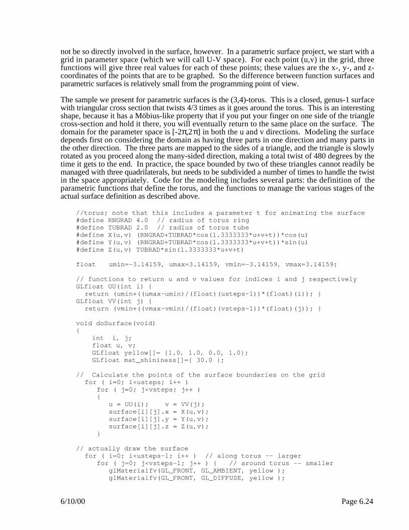
The sample we present for parametric surfaces is the (3,4)-torus. This is a closed, genus-1 surfacewith triangular cross section that twists 4/3 times as it goes around the torus. This is an interestingshape, because it has a Möbius-like property that if you put your finger on one side of the trianglecross-section and hold it there, you will eventually return to the same place on the surface. Thedomain for the parameter space is [-2π,2π] in both the u and v directions. Modeling the surfacedepends first on considering the domain as having three parts in one direction and many parts inthe other direction. The three parts are mapped to the sides of a triangle, and the triangle is slowlyrotated as you proceed along the many-sided direction, making a total twist of 480 degrees by thetime it gets to the end. In practice, the space bounded by two of these triangles cannot readily bemanaged with three quadrilaterals, but needs to be subdivided a number of times to handle the twistin the space appropriately. Code for the modeling includes several parts: the definition of theparametric functions that define the torus, and the functions to manage the various stages of theactual surface definition as described above.

//torus; note that this includes a parameter t for animating the surface#define RNGRAD 4.0 // radius of torus ring#define TUBRAD 2.0 // radius of torus tube#define X(u,v) (RNGRAD+TUBRAD*cos(1.3333333*u+v+t))*cos(u)#define Y(u,v) (RNGRAD+TUBRAD*cos(1.3333333*u+v+t))*sin(u)#define Z(u,v) TUBRAD*sin(1.3333333*u+v+t)

float umin=-3.14159, umax=3.14159, vmin=-3.14159, vmax=3.14159;

// functions to return u and v values for indices i and j respectivelyGLfloat UU(int i) {

return (umin+((umax-umin)/(float)(usteps-1))*(float)(i)); }GLfloat VV(int j) {

return (vmin+((vmax-vmin)/(float)(vsteps-1))*(float)(j)); }

void doSurface(void){ int i, j; float u, v; GLfloat yellow[]= {1.0, 1.0, 0.0, 1.0}; GLfloat mat_shininess[]={ 30.0 };

// Calculate the points of the surface boundaries on the gridfor ( i=0; i<usteps; i++ )

for ( j=0; j<vsteps; j++ ){

u = UU(i); v = VV(j);surface[i][j].x = X(u,v);surface[i][j].y = Y(u,v);surface[i][j].z = Z(u,v);

}

// actually draw the surfacefor ( i=0; i<usteps-1; i++ ) // along torus -- larger

for ( j=0; j<vsteps-1; j++ ) { // around torus -- smallerglMaterialfv(GL_FRONT, GL_AMBIENT, yellow );glMaterialfv(GL_FRONT, GL_DIFFUSE, yellow );

6/10/00 Page 6.25

glMaterialfv(GL_BACK, GL_AMBIENT, yellow );glMaterialfv(GL_BACK, GL_DIFFUSE, yellow );glMaterialfv(GL_FRONT_AND_BACK, GL_SHININESS, mat_shininess );doQuad(20,1,surface[i][j],surface[i+1][j],

surface[i][j+1], surface[i+1][j+1]);}

}

// Divide quad into m strips vertically and images each separately.void doQuad(int n,int m,surfpoint p0,surfpoint p1,surfpoint p2,surfpoint p3){

int i;surfpoint A, B, C, D; // A and B are the top points of each separate

// strip; C and D are the bottom points.

for (i=0; i<m; i++) {A.x = (p0.x*(float)(m-i) + p1.x*(float)i)/(float)m;A.y = (p0.y*(float)(m-i) + p1.y*(float)i)/(float)m;A.z = (p0.z*(float)(m-i) + p1.z*(float)i)/(float)m;B.x = (p0.x*(float)(m-i-1) + p1.x*(float)(i+1))/(float)m;B.y = (p0.y*(float)(m-i-1) + p1.y*(float)(i+1))/(float)m;B.z = (p0.z*(float)(m-i-1) + p1.z*(float)(i+1))/(float)m;

C.x = (p2.x*(float)(m-i) + p3.x*(float)i)/(float)m;C.y = (p2.y*(float)(m-i) + p3.y*(float)i)/(float)m;C.z = (p2.z*(float)(m-i) + p3.z*(float)i)/(float)m;D.x = (p2.x*(float)(m-i-1) + p3.x*(float)(i+1))/(float)m;D.y = (p2.y*(float)(m-i-1) + p3.y*(float)(i+1))/(float)m;D.z = (p2.z*(float)(m-i-1) + p3.z*(float)(i+1))/(float)m;doStrip(n, A, B, C, D);

}}

/* Now we have one vertical strip that we must subdivide into n pieces, each of which will be two triangles. We actually create a nx2 array of surfpoints, and then divide each quad going down the array into two triangles, each of which is "emitted" with its own function call.

*/

void doStrip(int n,surfpoint p0,surfpoint p1,surfpoint p2,surfpoint p3){

int i, j;surfpoint A, B, buffer[3];

for (i=0; i<=n; i++) {A.x = (p0.x*(float)(n-i) + p2.x*(float)i)/(float)n;A.y = (p0.y*(float)(n-i) + p2.y*(float)i)/(float)n;A.z = (p0.z*(float)(n-i) + p2.z*(float)i)/(float)n;B.x = (p1.x*(float)(n-i) + p3.x*(float)i)/(float)n;B.y = (p1.y*(float)(n-i) + p3.y*(float)i)/(float)n;B.z = (p1.z*(float)(n-i) + p3.z*(float)i)/(float)n;theStrip[i][0] = A;theStrip[i][1] = B;

}// now manipulate the strip to send out the triangles one at a time// to the actual output function, using a rolling buffer for points.buffer[0] = theStrip[0][0];buffer[1] = theStrip[0][1];

6/10/00 Page 6.26

for (i=1; i<=n; i++)for (j=0; j<2; j++) {

buffer[2] = theStrip[i][j];emit(buffer);buffer[0] = buffer[1];buffer[1] = buffer[2];

}}

// Handle one triangle as an array of three surfpoints.void emit( surfpoint *buffer ) {

surfpoint Normal, diff1, diff2;

diff1.x = buffer[1].x - buffer[0].x;diff1.y = buffer[1].y - buffer[0].y;diff1.z = buffer[1].z - buffer[0].z;diff2.x = buffer[2].x - buffer[1].x;diff2.y = buffer[2].y - buffer[1].y;diff2.z = buffer[2].z - buffer[1].z;Normal.x = diff1.y*diff2.z - diff2.y*diff1.z;Normal.y = diff1.z*diff2.x - diff1.x*diff2.z;Normal.z = diff1.x*diff2.y - diff1.y*diff2.x;glBegin(GL_POLYGON);

glNormal3f(Normal.x,Normal.y,Normal.z);glVertex3f(buffer[0].x,buffer[0].y,buffer[0].z);glVertex3f(buffer[1].x,buffer[1].y,buffer[1].z);glVertex3f(buffer[2].x,buffer[2].y,buffer[2].z);

glEnd();}

Figure 6.14: a parametric surface

The display of this surface in Figure 6.14 focuses on the surface shapes, which can be quitecomplex from certain viewpoints. Thus it is important to allow the student to have full rotation

6/10/00 Page 6.27

control in all three axes via the keyboard or the mouse. In addition, the surface rotates slowly inthe plane of the figure, emphasizing that the display is dynamic. Code for the animation is quiteroutine and is omitted.

The differences between function surfaces and parametric surfaces can be immense. Functionsurfaces are always single-sheet: they always look like a horizontal sheet that has been distortedupwards and downwards, but never wraps around on itself. Parametric surfaces can be muchmore complex. For example, a sphere can be seen as a parametric surface whose coordinates arecomputed from latitude and longitude, a two-dimensional region; a torus can be seen as aparametric surface whose coordinates are computed from the angular displacement around the torusand the angular displacement in the torus ring, another pair of dimensions. The figure aboveshows an example of a parametric surface that encloses a volume, surely something a functionsurface could never do.

Many simpler surfaces can be created using parametric definitions, and these make good studentprojects. It is easy to define a simple torus in this way, for example; the functions are

x(u,v)=(A+B*cos(v))*cos(u); y(u,v)=(A+B*cos(v))*sin(u); andz(u,v)=B*sin(v) for real constants A and B

for values of u and v between 0 and 2*π, where A is the radius of the torus body and B is theradius of the torus ring. Compare these equations with the ones used to define the figure aboveand note the similarity. Note also how defining a grid on the (u,v) domain corresponds to thedefinition of the torus in the GLUT torus model. Other examples may be considered as well; acouple of these that you may wish to experiment with are:

Helicoid:x(u,v)=a*u*cos(v), y(u,v)=b*u*sin(v); z(u,v)=c*v for real constants a, b, c

Conical spiral:x(u,v)=a*[1-(v/2*π)]*cos(n*v)*[1+cos(u)]+c*cos(n*v);

y(u,v)=a*[1-(v/2*π)]*sin(n*v)*[1+cos(u)]+c*sin(n*v);

z(u,v)=(b*v/2*π)+a*[1-v/(2*π)]*sin*u) for real constants a, b, c and integer n

This area of surface exploration offers some very interesting opportunities for advanced studies infunctions. For example, the parametric surface may not exist in 3-space but in higher-dimensionalspace, and then may be projected down into 3-space to be seen. For example, there may be four ormore functions of u and v representing four or more dimensions. Familiar surfaces such as Kleinbottles may be viewed this way, and it can be interesting to look at options in projections to 3-space as another way for the user to control the view.

Projects that simulate a scientific process

14. Gas laws

It is fairly simple to program a simulation of randomly-moving molecules in an enclosed space.This simulation models the behavior of gases in a container and can allow a student to consider therelationship between pressure and volume or pressure and temperature in the standard gas laws.These laws say that when temperature is held constant, pressure and volume vary inversely. Thesimulation can display the principles involved and can allow a user to query the system for theanalogs of temperature and pressure, getting back data that can be used in a statistical test of thelaw above.

6/10/00 Page 6.28

The simulation is straightforward: the student defines an initial space and creates a large number ofindividual points in that space. The idle callback gives each point a random motion with a knownaverage distance (simulating a fixed temperature) in a random direction. The space can be enlargedor shrunk. If the volume is shrunk, any points that might have been outside the new smaller spaceare moved back into the space; if the volume is expanded, points are allowed to move freely intothe new space. If the motion would take the point outside the space, that motion is reflected backinto the space and a “hit” is recorded to simulate pressure in the space. This count serves to modelthe pressure. So the student can use interactive controls to change the volume and observe thenumber of counts, testing the hypothesis that the number of counts increases inversely with thesurface area. The student could also change the average distance of a random motion, modelingtemperature changes, and test the hypothesis that the number of counts increases directly with thedistance (that is, the temperature). Information on the volume, collision count, or distance traveledcan be retrieved at any point by a simple keystroke. In fact, the small number of molecules in thissimulation give a very large variability of the product of surface area and collisions, so the studentwill need to do some sample statistics to test the hypothesis.

The computational model for this process is straightforward. The points are positioned at randominitial locations, and the idle callback handles motion of each particle in turn by generating arandom offset that changes the particle’s position. One particle has its motion tracked and a recordof its recent positions drawn to illustrate how the particles travel; the resulting track (the yellowtrack in the figure below) is a very good example of a random walk. The code for the trail for onepoint, for the idle callback, and for tallying the hits is:

// code for the trail of one pointglBegin(GL_POINTS);

for ( i=0; i<=NMOLS; i++ ) {glVertex3fv(mols[i]);if (i == 0) {

if (npoints < TRAILSIZE) npoints++;for (j=TRAILSIZE-1; j>0; j--)

for (k=0; k<3; k++)trail[j][k]=trail[j-1][k];

for (k=0; k<3; k++){trail[0][k] = mols[i][k];

}}

}

// the idle() callbackvoid animate(void){

int i,j,sign;

bounce = 0;for(i=0; i<NMOLS; i++) {

for (j=0; j<3; j++) {sign = -1+2*(rand()%2);mols[i][j] +=

(float)sign*distance*((float)(rand()%GRAN)/(float)(GRAN));if (mols[i][j] > bound)

{mols[i][j] = 2.0*bound - mols[i][j]; bounce++;}if (mols[i][j] <-bound)

{mols[i][j] = 2.0*(-bound) - mols[i][j]; bounce++;}}


6/10/00 Page 6.29

}

// tally the hits on the surface of the volumevoid tally(void){

float pressure, volume;

pressure = (float)bounce/(bound*bound); // hits per unit areavolume = bound*bound*bound; // dimension cubedprintf("pressure %f, volume %f, product %f\n",

pressure,volume,pressure*volume);}

A display of the volume and retrieved information is shown in Figure 6.15 below. This projectwould naturally use simple color and no lights; it should not even need to use hidden surfaces.

Figure 6.15: Displaying the gas as particles in the fixed space, with simulation printouts included

The display operates by providing a very rapid animation of the particles, so the user gets thestrong impression of molecules moving quickly within the space. It is possible to move the viewaround with the keyboard, and every time the user presses the ‘t’ key the program produces a tallysuch as that shown at the bottom of the figure. This the visual communication takes the form of anactual experiment that is probed at any time to read the current state. Of course, there are somepossible problems with the simulation; if the user expands the space quickly, it may take some timefor the particles to move out to the boundaries so the tallies are likely to be low for a while, and if

6/10/00 Page 6.30

the user contracts the space too quickly, the particles are seen outside the box for a short perioduntil they can be brought back inside.

One may properly ask why this simulation does not demonstrate the relationship between pressureand temperature in the gas laws. This is primarily because the simulation does not includecollisions between molecules. Adding this capability would require so much collision testing that itwould slow down the simulation and take away the real-time nature of the display.

15. Diffusion through a semipermeable membrane

One of the common processes in biological processes involves molecules transporting across semi-permeable membranes. These membranes will allow molecules to pass at varying rates, dependingon many factors. One of these factors is the molecular weight, where lighter molecules will passthrough a membrane more easily than heavier molecules. (A more realistic factor is the physicaldimension of the molecule, and this project can be re-phrased in terms of molecule size instead ofweight).

This project involves processes very much like the gas law simulation above, including randommotion of the molecules (represented as points), tracing the recent motion of molecules via rollingarrays, and the inclusion of a tally function. However, this simulation adds a plane between tworegions and simulates the behavior of a semipermeable membrane for molecules of two differentweights (here called “light” and “heavy” without any attempt to match the behaviors with those ofany real molecules and membranes).

The code we present for this concentrates on simulating the motion of the particles with specialattention to the boundaries of the space and the nature of the membrane, all contained in the idlecallback:

void animate(void){

#define HEAVYLEFT 0.8#define HEAVYRIGHT 0.9#define LIGHTLEFT 0.3#define LIGHTRIGHT 0.1

#define LEFT 0#define RIGHT 1int i,sign,whichside;

for(i=0; i<NHEAVY; i++) {if (heavy[i][0] < 0.0) whichside = LEFT; else whichside = RIGHT;sign = rand()%2; if (sign == 0) sign = -1;heavy[i][0] += sign*(float)(rand()%GRAN)/(float)(16*GRAN);sign = rand()%2; if (sign == 0) sign = -1;heavy[i][1] += sign*(float)(rand()%GRAN)/(float)(16*GRAN);sign = rand()%2; if (sign == 0) sign = -1;heavy[i][2] += sign*(float)(rand()%GRAN)/(float)(16*GRAN);if (heavy[i][0] > 1.0) heavy[i][0] = 2.0 - heavy[i][0];if ((whichside==RIGHT)&&(heavy[i][0] < 0.0)) // cross right to left?

if ( (float)(rand()%GRAN)/(float)(GRAN) >= HEAVYLEFT)heavy[i][0] = -heavy[i][0];

if ((whichside==LEFT)&&(heavy[i][0] > 0.0)) // cross left to right?if ( (float)(rand()%GRAN)/(float)(GRAN) >= HEAVYRIGHT)

heavy[i][0] = -heavy[i][0];if (heavy[i][0] > 1.0) heavy[i][0] = 2.0 - heavy[i][0];if (heavy[i][0] <-1.0) heavy[i][0] =-2.0 - heavy[i][0];

6/10/00 Page 6.31

if (heavy[i][1] > 1.0) heavy[i][1] = 2.0 - heavy[i][1];if (heavy[i][1] < 0.0) heavy[i][1] = -heavy[i][1];if (heavy[i][2] > 1.0) heavy[i][2] = 2.0 - heavy[i][2];if (heavy[i][2] < 0.0) heavy[i][2] = -heavy[i][2];

}for(i=0; i<NLIGHT; i++) {

if (light[i][0] < 0.0) whichside = LEFT; else whichside = RIGHT;sign = rand()%2; if (sign == 0) sign = -1;light[i][0] += sign*(float)(rand()%GRAN)/(float)(16*GRAN);sign = rand()%2; if (sign == 0) sign = -1;light[i][1] += sign*(float)(rand()%GRAN)/(float)(16*GRAN);sign = rand()%2; if (sign == 0) sign = -1;light[i][2] += sign*(float)(rand()%GRAN)/(float)(16*GRAN);if (light[i][0] > 1.0) light[i][0] = 2.0 - light[i][0];if ((whichside == RIGHT)&&(light[i][0] < 0.0))

if ( (float)(rand()%GRAN)/(float)(GRAN) >= LIGHTLEFT)light[i][0] = -light[i][0];

if ((whichside == LEFT)&&(light[i][0] > 0.0))if ( (float)(rand()%GRAN)/(float)(GRAN) >= LIGHTRIGHT)

light[i][0] = -light[i][0];if (light[i][0] <-1.0) light[i][0] =-2.0 - light[i][0];if (light[i][1] > 1.0) light[i][1] = 2.0 - light[i][1];if (light[i][1] < 0.0) light[i][1] = -light[i][1];if (light[i][2] > 1.0) light[i][2] = 2.0 - light[i][2];if (light[i][2] < 0.0) light[i][2] = -light[i][2];


}

This display, shown in Figure 6.16, has with pretty effective animation of the particles and allowsthe user to rotate the simulation region to view the behavior from any direction. The programpresents the tally results in a separate text-output region which is included with the figure at leftbelow. The tallys were taken at one-minute intervals to illustrate that the system settles into a fairlyconsistent steady-state behavior over time, certainly something that one would want in asimulation. The membrane is presented with partial transparency so that the user gets a sense ofseeing into the whole space when viewing the simulation with arbitrary rotations.

Figure 6.16: display of the diffusion simulation, directly across the membrane at left (includingdata output from the simulation), and in a view oriented to show the membrane itself at right.

6/10/00 Page 6.32

Projects that illustrate dynamic systems

16. The Lorenz attractor

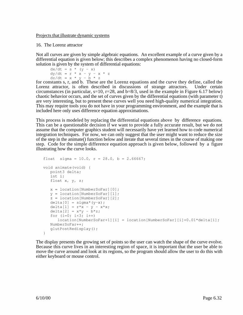
Not all curves are given by simple algebraic equations. An excellent example of a curve given by adifferential equation is given below; this describes a complex phenomenon having no closed-formsolution is given by the system of differential equations:

dx/dt = s * (y - x)dy/dt = r * x - y - x * zdz/dt = x * y - b * z

for constants s, r, and b. These are the Lorenz equations and the curve they define, called theLorenz attractor, is often described in discussions of strange attractors. Under certaincircumstances (in particular, s=10, r=28, and b=8/3, used in the example in Figure 6.17 below)chaotic behavior occurs, and the set of curves given by the differential equations (with parameter t)are very interesting, but to present these curves well you need high-quality numerical integration.This may require tools you do not have in your programming environment, and the example that isincluded here only uses difference equation approximations.

This process is modeled by replacing the differential equations above by difference equations.This can be a questionable decision if we want to provide a fully accurate result, but we do notassume that the computer graphics student will necessarily have yet learned how to code numericalintegration techniques. For now, we can only suggest that the user might want to reduce the sizeof the step in the animate() function below and iterate that several times in the course of making onestep. Code for the simple difference equation approach is given below, followed by a figureillustrating how the curve looks.

float sigma = 10.0, r = 28.0, b = 2.66667;

void animate(void) {point3 delta;int i;float x, y, z;

x = location[NumberSoFar][0];y = location[NumberSoFar][1];z = location[NumberSoFar][2];delta[0] = sigma*(y-x);delta[1] = r*x - y - x*x;delta[2] = x*y - b*z;for (i=0; i<3; i++)

location[NumberSoFar+1][i] = location[NumberSoFar][i]+0.01*delta[i];NumberSoFar++;glutPostRedisplay();

}

The display presents the growing set of points so the user can watch the shape of the curve evolve.Because this curve lives in an interesting region of space, it is important that the user be able tomove the curve around and look at its regions, so the program should allow the user to do this witheither keyboard or mouse control.

6/10/00 Page 6.33

Figure 6.17: the Lorenz curve

17. The Sierpinski attractor

Sometimes an attractor is a more complex object than the curve of the Lorenz attractor. Let usconsider a process in which some bouned space contains four designated points that are thevertices of a tetrahedron (regular or not), and let us put a large number of other points into thatspace. Now define a process in which for each non-designated point, a random designated point ischosen and the non-designated point is moved to the point precisely halfway between its originalposition and the position of the designated point. Apply that process repeatedly. It may not seemthat any order would arise from the original chaos, but it does — and in fact there is a specificregion of space into which each of the points tends, and from which it can never escape. This iscalled the Sierpinski attractor, and it is shown in Figure 6.18.

Figure 6.18: the Sierpinski attractor

The Sierpinski attractor is also interesting because it can be defined in a totally different way. If werecursively define a tetrahedron to be displayed as a collection of four tetrahedra, each of half theheight of the original tetrahedron, each touching all the others at precisely one point, and eachhaving one of the vertices of the original tetrahedron, then the limit of this definition is the attractoras defined and presented above.

6/10/00 Page 6.34

Some enhancements to the display

Stereo pairs

If you create a window that is twice as wide as it is high, and if you divide it into left and rightviewports, you can display two images in the window simultaneously. If these two images arecreated with the same model and same center of view, but with two eye points that simulate thelocation of two eyes, then the images simulate those seen by a person’s two eyes. Finally, if thewindow is relatively small and the distance between the centers of the two viewports is reasonablyclose to the distance between a person’s eyes, then the viewer can probably resolve the two imagesinto a single image and see a genuine 3D view. Such a view is shown in Figure 6.19 below: a pairof views of psilocybin.mol, one of the molecules included in thise materials that has some 3Dinterest. None of these processes are difficult, so it would add some extra interest to include 3Dviewing in the molecule display project or almost any other of these projects.

Figure 6.19: A stereo pair that the viewer may be able to resolve.

The code below manages the two viewports and performs the display in each; the display portion isnot presented in order to keep the code short and to focus on the dual-viewport approach. Thiscreates two viewports, defines them to have different viewing projections, performs the sameactual display operations (indicated by the ellipsis) on each, and then presents the completeddisplay of both viewports at once to avoid the flicker of updating each separately.

void display( void ){// eye offset from center

float offset = 1.0;

// left-hand viewportglViewport(0,0,300,300);glClear(GL_COLOR_BUFFER_BIT | GL_DEPTH_BUFFER_BIT);glMatrixMode(GL_MODELVIEW);glLoadIdentity();gluLookAt(-offset, 0.0, ep, 0.0, 0.0, 0.0, 0.0, 1.0, 0.0);...

// right-hand viewportglViewport(300,0,300,300);glClear(GL_COLOR_BUFFER_BIT | GL_DEPTH_BUFFER_BIT);glMatrixMode(GL_MODELVIEW);

6/10/00 Page 6.35

glLoadIdentity();gluLookAt(offset, 0.0, ep, 0.0, 0.0, 0.0, 0.0, 1.0, 0.0);...glutSwapBuffers();

}

A more complex kind of display — Chromadepth™ display — depends on texture mapping andwill be described later.

Credits:

A number of colleagues have helped with graphical concepts, with scientific principles, or withmodels of the scientific issues. We apologize in advance for those we may miss, but we want tothank Michael J. Bailey of the San Diego Supercomputer Center (SDSC) for many fruitfuldiscussions across all of these topics, and with Kris Stewart of San Diego State University(SDSU), Angela Shiflet of Wofford College, Rozeanne Steckler and Kim Baldridge of SDSU, andIan Littlewood of California State University Stanislaus for their contributions in one or more ofthese areas.

References:• Zimmermann, Walter and Steve Cunningham, Visualization in Teaching and Learning

Mathematics, MAA Notes Number 19, Mathematical Association of America, 1991• Banchoff, Tom et al., “Student-Generated Software for Differential Geometry,” in

Zimmermann and Cunningham, above, pp. 165-171• von Seggern, David, CRC Standard Curves and Surfaces, CRC Press, 1993• Textbook for multivariate calculus ...• Textbook for differential geometry? ...• Chromadepth glasses and other information are available from

Chromatek Inc1246 Old Alpharetta RoadAlpharetta, GA 30005888-669-8233http://www.chromatek.com/

6/10/00 Page 6.36

Appendix I: PDB file format

The national Protein Data Bank (PDB) file format is extremely complex and contains much moreinformation than we can ever hope to use for student projects. We will extract the information weneed for simple molecular display from the reference document on this file format to present here.From the chemistry point of view, the student might be encouraged to look at the longer filedescription to see how much information is recorded in creating a full record of a molecule.

There are two kinds of records in a PDB file that are critical to us: atom location recordsand bond description records. These specify the atoms in the molecule and the bonds betweenthese atoms. By reading these records we can fill in the information in the internal data structuresthat hold the information needed to generate the display. The information given here on the atomlocation (ATOM) and bond description (CONECT) records is from the reference. There is anotherkind of record that describes atoms, with the keyword HETATM, but we leave this description tothe full PDB format manual in the references.

ATOM records: The ATOM records present the atomic coordinates for standard residues, inangstroms. They also present the occupancy and temperature factor for each atom. The elementsymbol is always present on each ATOM record.

Record Format:COLUMNS DATA TYPE FIELD DEFINITION------------------------------------------------------------------------------ 1 - 6 Record name "ATOM " 7 - 11 Integer serial Atom serial number.13 - 16 Atom name Atom name.17 Character altLoc Alternate location indicator.18 - 20 Residue name resName Residue name.22 Character chainID Chain identifier.23 - 26 Integer resSeq Residue sequence number.27 AChar iCode Code for insertion of residues.31 - 38 Real(8.3) x Orthogonal coordinates for X in Angstroms.39 - 46 Real(8.3) y Orthogonal coordinates for Y in Angstroms.47 - 54 Real(8.3) z Orthogonal coordinates for Z in Angstroms.55 - 60 Real(6.2) occupancy Occupancy.61 - 66 Real(6.2) tempFactor Temperature factor.73 - 76 LString(4) segID Segment identifier, left-justified.77 - 78 LString(2) element Element symbol, right-justified.79 - 80 LString(2) charge Charge on the atom.

The "Atom name" field can be complex, because there are other ways to give names than thestandard atomic names. In the PDB file examples provided with this set of projects, we have beencareful to avoid names that differ from the standard names in the periodic table, but that means thatwe have not been able to use all the PDB files from, say, the chemical data bank. If yourchemistry program wants you to use a particular molecule as an example, but that example’s datafile uses other formats for atom names in its file, you will need to modify the readPDBfile()function of these examples.

Example: 1 2 3 4 5 6 7 812345678901234567890123456789012345678901234567890123456789012345678901234567890ATOM 1 C 1 -2.053 2.955 3.329 1.00 0.00ATOM 2 C 1 -1.206 3.293 2.266 1.00 0.00ATOM 3 C 1 -0.945 2.371 1.249 1.00 0.00ATOM 4 C 1 -1.540 1.127 1.395 1.00 0.00ATOM 5 C 1 -2.680 1.705 3.426 1.00 0.00

6/10/00 Page 6.37

ATOM 6 C 1 -2.381 0.773 2.433 1.00 0.00ATOM 7 O 1 -3.560 1.422 4.419 1.00 0.00ATOM 8 O 1 -2.963 -0.435 2.208 1.00 0.00ATOM 9 C 1 -1.455 -0.012 0.432 1.00 0.00ATOM 10 C 1 -1.293 0.575 -0.967 1.00 0.00ATOM 11 C 1 -0.022 1.456 -0.953 1.00 0.00ATOM 12 C 1 -0.156 2.668 0.002 1.00 0.00ATOM 13 C 1 -2.790 -0.688 0.814 1.00 0.00ATOM 14 C 1 -4.014 -0.102 0.081 1.00 0.00ATOM 15 C 1 -2.532 1.317 -1.376 1.00 0.00ATOM 16 C 1 -3.744 1.008 -0.897 1.00 0.00ATOM 17 O 1 -4.929 0.387 1.031 1.00 0.00ATOM 18 C 1 -0.232 -0.877 0.763 1.00 0.00ATOM 19 C 1 1.068 -0.077 0.599 1.00 0.00ATOM 20 N 1 1.127 0.599 -0.684 1.00 0.00ATOM 21 C 1 2.414 1.228 -0.914 1.00 0.00ATOM 22 H 1 2.664 1.980 -0.132 1.00 0.00ATOM 23 H 1 3.214 0.453 -0.915 1.00 0.00ATOM 24 H 1 2.440 1.715 -1.915 1.00 0.00ATOM 25 H 1 -0.719 3.474 -0.525 1.00 0.00ATOM 26 H 1 0.827 3.106 0.281 1.00 0.00ATOM 27 H 1 -2.264 3.702 4.086 1.00 0.00ATOM 28 H 1 -0.781 4.288 2.207 1.00 0.00ATOM 29 H 1 -0.301 -1.274 1.804 1.00 0.00ATOM 30 H 1 -0.218 -1.756 0.076 1.00 0.00ATOM 31 H 1 -4.617 1.581 -1.255 1.00 0.00ATOM 32 H 1 -2.429 2.128 -2.117 1.00 0.00ATOM 33 H 1 -4.464 1.058 1.509 1.00 0.00ATOM 34 H 1 -2.749 -1.794 0.681 1.00 0.00ATOM 35 H 1 1.170 0.665 1.425 1.00 0.00ATOM 36 H 1 1.928 -0.783 0.687 1.00 0.00ATOM 37 H 1 -3.640 2.223 4.961 1.00 0.00ATOM 38 H 1 0.111 1.848 -1.991 1.00 0.00ATOM 39 H 1 -1.166 -0.251 -1.707 1.00 0.00ATOM 40 H 1 -4.560 -0.908 -0.462 1.00 0.00

CONECT records: The CONECT records specify connectivity between atoms for whichcoordinates are supplied. The connectivity is described using the atom serial number as found inthe entry.

Record Format:COLUMNS DATA TYPE FIELD DEFINITION---------------------------------------------------------------------------- 1 - 6 Record name "CONECT" 7 - 11 Integer serial Atom serial number12 - 16 Integer serial Serial number of bonded atom17 - 21 Integer serial Serial number of bonded atom22 - 26 Integer serial Serial number of bonded atom27 - 31 Integer serial Serial number of bonded atom32 - 36 Integer serial Serial number of hydrogen bonded atom37 - 41 Integer serial Serial number of hydrogen bonded atom42 - 46 Integer serial Serial number of salt bridged atom47 - 51 Integer serial Serial number of hydrogen bonded atom52 - 56 Integer serial Serial number of hydrogen bonded atom57 - 61 Integer serial Serial number of salt bridged atom

Example:

6/10/00 Page 6.38

1 2 3 4 5 6 71234567890123456789012345678901234567890123456789012345678901234567890CONECT 1179 746 1184 1195 1203CONECT 1179 1211 1222CONECT 1021 544 1017 1020 1022 1211 1222 1311

As we noted at the beginning of this Appendix, PDB files can be extremely complex, and most ofthe examples we have found have been fairly large. The file below is among the simplest PDBfiles we've seen, and describes the adrenalin molecule. This is among the materials provided asadrenaline.pdb.

HEADER NONAME 08-Apr-99 NONE 1TITLE NONE 2AUTHOR Frank Oellien NONE 3REVDAT 1 08-Apr-99 0 NONE 4ATOM 1 C 0 -0.017 1.378 0.010 0.00 0.00 C+0ATOM 2 C 0 0.002 -0.004 0.002 0.00 0.00 C+0ATOM 3 C 0 1.211 -0.680 -0.013 0.00 0.00 C+0ATOM 4 C 0 2.405 0.035 -0.021 0.00 0.00 C+0ATOM 5 C 0 2.379 1.420 -0.013 0.00 0.00 C+0ATOM 6 C 0 1.169 2.089 0.002 0.00 0.00 C+0ATOM 7 O 0 3.594 -0.625 -0.035 0.00 0.00 O+0ATOM 8 O 0 1.232 -2.040 -0.020 0.00 0.00 O+0ATOM 9 C 0 -1.333 2.112 0.020 0.00 0.00 C+0ATOM 10 O 0 -1.177 3.360 0.700 0.00 0.00 O+0ATOM 11 C 0 -1.785 2.368 -1.419 0.00 0.00 C+0ATOM 12 N 0 -3.068 3.084 -1.409 0.00 0.00 N+0ATOM 13 C 0 -3.443 3.297 -2.813 0.00 0.00 C+0ATOM 14 H 0 -0.926 -0.557 0.008 0.00 0.00 H+0ATOM 15 H 0 3.304 1.978 -0.019 0.00 0.00 H+0ATOM 16 H 0 1.150 3.169 0.008 0.00 0.00 H+0ATOM 17 H 0 3.830 -0.755 -0.964 0.00 0.00 H+0ATOM 18 H 0 1.227 -2.315 -0.947 0.00 0.00 H+0ATOM 19 H 0 -2.081 1.509 0.534 0.00 0.00 H+0ATOM 20 H 0 -0.508 3.861 0.214 0.00 0.00 H+0ATOM 21 H 0 -1.037 2.972 -1.933 0.00 0.00 H+0ATOM 22 H 0 -1.904 1.417 -1.938 0.00 0.00 H+0ATOM 23 H 0 -3.750 2.451 -1.020 0.00 0.00 H+0ATOM 24 H 0 -3.541 2.334 -3.314 0.00 0.00 H+0ATOM 25 H 0 -4.394 3.828 -2.859 0.00 0.00 H+0ATOM 26 H 0 -2.674 3.888 -3.309 0.00 0.00 H+0CONECT 1 2 6 9 0 NONE 31CONECT 2 1 3 14 0 NONE 32CONECT 3 2 4 8 0 NONE 33CONECT 4 3 5 7 0 NONE 34CONECT 5 4 6 15 0 NONE 35CONECT 6 5 1 16 0 NONE 36CONECT 7 4 17 0 0 NONE 37CONECT 8 3 18 0 0 NONE 38CONECT 9 1 10 11 19 NONE 39CONECT 10 9 20 0 0 NONE 40CONECT 11 9 12 21 22 NONE 41CONECT 12 11 13 23 0 NONE 42CONECT 13 12 24 25 26 NONE 43END NONE 44

Figure: Example of a simple molecule file in PDB format

Reference:Protein Data Bank Contents Guide: Atomic Coordinate Entry Format Description, version 2.1,available online from http://www.pdb.bnl.gov

6/10/00 Page 6.39

Appendix II: CTL file format

The structure of the CT file is straightforward. The file is segmented into several parts, including aheader block, the counts line, the atom block, the bond block, and other information. The headerblock is the first three lines of the file and include the name of the molecule (line 1); the user’sname, program, date, and other information (line 2); and comments (line 3). The next line of thefile is the counts line and contains the number of molecules and the number of bonds as the firsttwo entries. The next set of lines is the atom block that describes the properties of individual atomsin the molecule; each contains the X-, Y-, and Z-coordinate and the chemical symbol for anindividual atom. The next set of lines is the bonds block that describes the properties of individualbonds in the molecule; each line contains the number (starting with 1) of the two atoms making upthe bond and an indication of whether the bond is single, double, triple, etc. After these lines aremore lines with additional descriptions of the molecule that we will not use for this project. Anexample of a simple CTfile-format file for a molecule (from the reference) is given in Figure A-1below.

Obviously there are many pieces of information in the file that are of interest to the chemist,and in fact this is an extremely simple example of a file. But for our project we are only interestedin the geometry of the molecule, so the additional information in the file must be skipped when thefile is read.

L-Alanine (13C)GSMACCS-II10169115362D 1 0.00366 0.00000 0

6 5 0 0 1 0 3 V2000-0.6622 0.5342 0.0000 C 0 0 2 0 0 0 0.6220 -0.3000 0.0000 C 0 0 0 0 0 0-0.7207 2.0817 0.0000 C 1 0 0 0 0 0-1.8622 -0.3695 0.0000 N 0 3 0 0 0 0 0.6220 -1.8037 0.0000 O 0 0 0 0 0 0 1.9464 0.4244 0.0000 O 0 5 0 0 0 01 2 1 0 0 01 3 1 1 0 01 4 1 0 0 02 5 2 0 0 02 6 1 0 0 0M CHG 2 4 1 6 -1M ISO 1 3 13M END

Figure: Example of a simple molecule file in CTfile format

Reference:CTFile Formats, MDL Information Systems, Inc., San Leandro, CA 94577, 1999. Availableby download from http://www.mdli.com/

Science Projects - California State University, Stanislaus

Documents

Transcript of Science Projects - California State University, Stanislaus