Science of the Total Environment 544 (2016) 883–891

Contents lists available at ScienceDirect

Science of the Total Environment

j ourna l homepage: www.e lsev ie r .com/ locate /sc i totenv

Mapping geogenic radon potential by regression kriging

László Pásztor a, Katalin Zsuzsanna Szabó b,⁎, Gábor Szatmári a, Annamária Laborczi a, Ákos Horváth c

a Institute for Soil Sciences and Agricultural Chemistry, Centre for Agricultural Research, Hungarian Academy of Sciences, Department of Environmental Informatics, Herman Ottó út 15, 1022 Bu-dapest, Hungaryb Department of Chemistry, Institute of Environmental Science, Szent István University, Páter Károly u. 1, Gödöllő 2100, Hungaryc Department of Atomic Physics, Eötvös University, Pázmány Péter sétány 1/A, 1117 Budapest, Hungary

H I G H L I G H T S G R A P H I C A L A B S T R A C T

• A new method, regression-kriging (RK)was tested for GRP mapping.

• Usage of spatially exhaustive, auxiliarydata on soil, geology, topography, landuse and climate.

• Inherent accuracy assessment (bothglobal and local).

• Interval estimation for the spatial exten-sion of the areas of GRP risk categories.

• Significance of fluvial sedimentary rock,pyroclast and land use properties on ra-don risk.

⁎ Corresponding author.E-mail address: sz_k_zs@yahoo.de (K.Z. Szabó).

http://dx.doi.org/10.1016/j.scitotenv.2015.11.1750048-9697/© 2015 Elsevier B.V. All rights reserved.

a b s t r a c t

a r t i c l e i n f o

Article history:Received 26 August 2015Received in revised form 27 November 2015Accepted 30 November 2015Available online xxxx

Editor: Tack F.M.

Radon (222Rn) gas is produced in the radioactive decay chain of uranium(238U)which is an element that is naturallypresent in soils. Radon is transported mainly by diffusion and convection mechanisms through the soil dependingmainly on the physical andmeteorological parameters of the soil and can enter and accumulate in buildings. Healthrisks originating from indoor radon concentration can be attributed to natural factors and is characterized bygeogenic radon potential (GRP). Identification of areaswith high health risks require spatial modeling, that is, map-ping of radon risk. In addition to geology andmeteorology, physical soil properties play a significant role in the de-termination of GRP. In order to compile a reliable GRP map for a model area in Central-Hungary, spatial auxiliaryinformation representing GRP forming environmental factors were taken into account to support the spatial infer-ence of the locallymeasuredGRP values. Since thenumber ofmeasured siteswas limited, efficient spatial predictionmethodologies were searched for to construct a reliable map for a larger area. Regression kriging (RK) was appliedfor the interpolation using spatially exhaustive auxiliary data on soil, geology, topography, land use and climate. RKdivides the spatial inference into twoparts. Firstly, the deterministic component of the target variable is determinedby a regression model. The residuals of the multiple linear regression analysis represent the spatially varying butdependent stochastic component,which are interpolated bykriging. Thefinalmap is the sumof the two componentpredictions. Overall accuracy of themapwas tested by Leave-One-Out Cross-Validation. Furthermore the spatial re-liability of the resultantmap is also estimated by the calculation of the 90%prediction interval of the local predictionvalues. The applicability of the applied method as well as that of the map is discussed briefly.

© 2015 Elsevier B.V. All rights reserved.

Keywords:Soil gas radonSpatial predictionAuxiliary environmental variablesRegression krigingPhysical soil properties

884 L. Pásztor et al. / Science of the Total Environment 544 (2016) 883–891

1. Introduction

Natural radon (222Rn) is a radioactive noble gas occurring in everysoil due to the radium (226Ra) and uranium (238U) content of the litho-sphere. Since radon is an inert gas it can easily enter from the soil intobuildings and its daughter isotopes can cause damage to lung tissue.This process produces more than half the average natural dose forhumans (2.4mSv y−1) (UNSCEAR, 2008). The impact of radon onhealthis highlighted by EU datawhich state that about 20,000 people die everyyear in the EU (Darby et al., 2005) due to elevated indoor radon concen-tration. Radon concentration shows a wide distribution in the soil. Insome areas as high as ten times the average readings can be measured.

In several countries a number of regulations were adopted andcountrywide surveys were launched to identify radon prone areas(Gue, 2015). The idea of the geogenic map is to visualize the purely nat-ural radon hazard, i.e. independently of anthropogenic factorswhich aresubject to secular changes, as building styles and living habits changewith time and also vary regionally, while the geogenic radon potential(GRP) is constant over geological eras (Bossew et al., 2013). The basicconcept of a geogenic radon prone area is a region where for natural,i.e. geogenic reasons, elevated indoor radon levels and elevated proba-bility of their occurrence must be expected (Bossew, 2014). Thegeogenic source of this hazard (or potential risk) at a location or overan area is described by its radon potential. Knowing the GRP of anarea one can decide whether the area should be investigated in detailor the assessment of the site of new buildings is necessary.

There are a lot of methods to define and map the physical quantitygeogenic radon potential (GRP) of an area. These methods are basedon several measured parameters as numerical (such as permeability,radon concentration in soil air, and 226Ra concentration) or geological,lithological data as categorical controls (Bossew et al., 2013). One ofthe internationally recognized approaches to quantify the GRP for thegeogenic radon map of Europe is the continuous variable (formerlyradon index) developed by Neznal et al. (2004), which is based onfield measurements of the radon concentration in soil gas and the gaspermeability of soils. This conventional continuous variable approachwas applied for several areas of Hungary and the Czech Republic, too(Neznal et al., 2004; Szabó et al., 2014). In a different approach, multi-variate classification, one cross-tabulates physical, mostly categoricalfactors which control the concept of the RP. The entries of the (possiblymulti-dimensional) table are classified into RP classes. These factors aretypically base and surface geology, geology, granulometry (as a proxy ofpermeability), hydrological properties, tectonics, and occurrence of“special features” such as caves, mines or other anthropogenicallymodified conditions which may enhance or reduce the natural RP.One elaborated example of this approach has been presented byFriedmann (2005).

At the same time several studies have shown the importance of theinfluence of soil physical parameters on the soil gas radon concentra-tion. The effect of moisture content and grain size on radon emanation(radon escape from grain to the pore space) is well investigatedwith macroscopic soil models (Sakoda et al., 2010, Schumann andGundersen, 1996). The emanation coefficient is higher where themois-ture content is higher because the radon diffusion length is about 600times lower (0.1 μm) in water than in air (63 μm) (Tanner, 1980).Thus radon atoms will remain in the pores (in the water) and couldnot reach another grain. Faheem and Matiullah (2008) investigatedthe moisture dependence of radon exhalation of several soils in labora-tory measurements. Radon exhalation rate (radon escape from grain tothe surface)was found to increasewith an increase inmoisture, reachedits maximum value and then decreased with further increase in thewater content. Schweikani et al. (1995) found that the increase in themoisture content causes a reduction in the radon diffusion since thepores through which radon diffuses is filled with water. Also they con-cluded that the degree of moisture saturation of the interstitial voidspace is the important factor rather than the moisture content as a

percentage of the dry weight and/or the porosity of soil. The degree ofmoisture saturation is closely related to physical soil properties suchas soil texture.

It is possible to establish accurate and robust estimation of specificderivatives by selected soil parameters using suitable pedo-radon trans-fer functions (PRTF). In this case more easily available soil maps andspatial databases can be used for the compilation of radon potentialmaps. Kemski et al. (2001) used an empirical ranking classification forthe classification of geogenic radon potential due to the lack of exactfunctional relationship between radon concentration in soil gas andair permeability. Ielsch et al. (2002) emphasized the complicated inter-actions between the different pedological factors and radon exhalation,which preferably leads to statistically based models. Sun et al. (2004)found that radon exhalation from soil and soil radon concentration aremore easily impacted by soil characters and they change in a ratherlarge range. Winkler et al. (2001) investigated the spatial and temporalvariability of the soil 222Rn concentration at field scale for rathersmall pilot areas. They found significant differences in the case of vari-ous soil conditions. Oliver and Khayrat (2001) focused their investiga-tion on the spatial variation of radon concentration in soil. Theyemphasized that appropriate information about the spatial scales ofradon variation in soil is needed to effectively sample for its spatial pre-diction, that is, mapping. Buttafuoco et al. (2007) tested variousgeostatistical methods (ordinary kriging, lognormal kriging, ordinarymulti-Gaussian kriging, and ordinary indicator cokriging) to study spa-tial structure of radon concentration for mapping purposes. The testedmethods did not use environmental co-variables for the spatial infer-ence. Multi-Gaussian kriging proved to be the most accurate methodof the considered interpolation techniques.

Sampling based mapping is inherently predictive, the value or classof the mapped variable can only be estimated at unvisited locations(Gessler et al., 1995; Scull et al., 2003). Spatial prediction can be carriedout (i) taking exclusively the mapped variable into consideration basedon its spatial features; (ii) also based on the mapped variable, but theconstraints of spatial validity are provided by further spatial, ancillaryinformation; (iii) in every predicted location supported by environmen-tal, auxiliary co-variables (McKenzie and Ryan, 1999).

Geology, climate, physical soil properties and radiological data arethe main GRP forming environmental factors. Spatial exhaustiveinformation on them is available relatively more easily. Thus spatialinference of locally measured GRP values can rely on methods whichexploit their existence.

Regression Kriging (RK;Hengl, 2009) is a spatial prediction techniquethat combines the regression of the dependent variable on auxiliary var-iableswith kriging of the regression residuals. It ismathematically equiv-alent to the interpolation method variously called universal kriging andkriging with external drift. (Hengl et al., 2004). Essentially, RK respectsthis fact, neither environmental correlation nor pure geostatistical inter-polation (simple, ordinary kriging) alone is able to account for thewholespatial variation that is to produce approximately perfect map products.They can be used as complementary spatial inference approaches whereone can improve the other's drawbacks.

The main objective of the study has been to test a new method ofGRP spatial prediction provided by regression-kriging (RK) usingspatially exhaustive auxiliary environmental variables (geology, soilphysical properties, topography, land use and climate). The expected re-sult has been a more detailed map than previous maps based on spatialresolution of the selected auxiliary variables. A further aim has been todetermine the performance and uncertainty of the method.

2. Materials and methods

2.1. Study area

The study area is located in the Pannonian Basin, in Central Hungaryand includes Budapest, themajority of Pest County and some surrounding

885L. Pásztor et al. / Science of the Total Environment 544 (2016) 883–891

areas (Fig. 1). The study area encompasses 5400 km2 covering 6.5% of thecountry. This part of Hungary has the highest population density. 28%(2.83 million) of the population of the country (9.9 million) live in the220 settlements of the study area. The area is also characterizedbydiversegeological and pedological environment, thus providing excellent condi-tions for radon risk mapping and geological modeling research.

The diverse geological background can be related to the joiningpointof the two highest Hungarian mountain ranges, the North HungarianMountains and the TransdanubianMountainswith the Great HungarianPlain. Accordingly, there are hills (the highest elevation is 938 m asl.)along the longitudinal extension (N–S direction) in the western partof the area. The River Danube enters the study area from the west andsharply turns to the south at the Danube Bend, an intense tourist area.The northeast part is hilly (Cserhát Mts. and Gödöllő Hills with thehighest elevation 652 and 345 m asl., respectively). The northwesternpart of the Great Hungarian Plain, the Pest Plain covers the middle andsouthern parts (100–150 m asl.) of the study area (Fig. 1).

Hungary has a temperate continental climate with a long-term an-nual average temperature of 11 °C with warm summers (20 °C), coldwinters (0 °C) and mild springs and autumns (10 °C). The annual aver-age precipitation is 500–550 mm. The precipitation falls mostly duringthe summermonths (especially June) and the least in thewinter season(especially February) based on the Hungarian Meteorological Service(OMSZ) database.

2.2. Data collection

In the present mapping approach we used a subset of our formerstudy (Szabó et al., 2014). Original locations of measurements containtwo densely sampled areas (two settlements). In order to apply regres-sion kriging efficiently, we filtered the original dataset. We onlyincluded two representative locations per settlement. Additionally twolocations were left out which were outside Hungary, since the auxiliaryenvironmental data were available only for Hungary. Altogether 145locations were involved in the analyses. These GRP data are based on

Fig. 1. The location o

field measured soil gas radon activity concentration and soil gaspermeability.

Soil gas radon activity concentration was measured in situ with aRAD7 Electronic Radon Detector (Durridge Company Inc., 2000)coupled with a soil probe. Soil gas was pumped out from (if possible)generally 0.8 m depth of the soil. The standard “Grab” sampling lasted20 min. Soil gas radon activity concentration was determined from the3-min half-life 218Po alpha peak at 6.0MeV and gives radon activity con-centration in Bq m−3 units. The rate of flow of the pump is 1 L min−1.The RAD7was calibrated in 2009 and the calibration is highly stable ac-cording to the manufacturer's specifications (Durridge Company Inc.,2000). Typical drift is less than 2% per year. The uncertainty (two-sigma) of RAD7 with a 5-min counting cycle is about 40%, 10%, 8% and5% in the case of 1, 10, 20, 40 kBq m−3 radon activity concentrationvalues, respectively.

Soil gas permeability measurement was performed immediatelyafter the soil gas radon measurement by Radon-JOK equipment(Radon v.o.s.) using the same soil probe. Calculation of the gas perme-ability was based on Darcy's equation (Koorevaar et al., 1983) accordingto the equipmentmanual (Radon v.o.s.). The equipmentworks bywith-drawing air by the application of negative pressure. Air is pumped fromthe soil under constant pressure through the probe with a constantcontact between the probe head and the soil. The soil is assumed to behomogeneous and isotropic with standard conditions prevailing. Fur-thermore, the air is assumed to be incompressible (pressure differencesare very much smaller than atmospheric pressure).

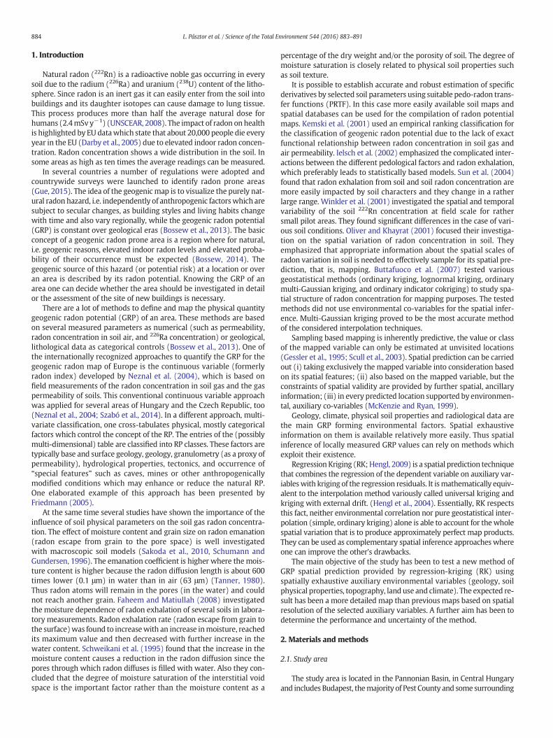
Site selection followed stratified, conditional random sampling. Theinternationally suggested 10 × 10 km grid for the European indoorradon map (Dubois et al., 2010; Tollefsen et al., 2011) represented theuniform strata of the sampling (Fig. 2). The conditions of site selectionwere the extension of geological formations and the distribution of set-tlements (built-up areas). On average, three measurement sites wereassigned in each cell sampling the three dominating geological forma-tions of the cell, also taking the locality of the towns into account. Wepreferred geological formations inside and around the settlementssince these are the target areas for planned building developments.

f the study area.

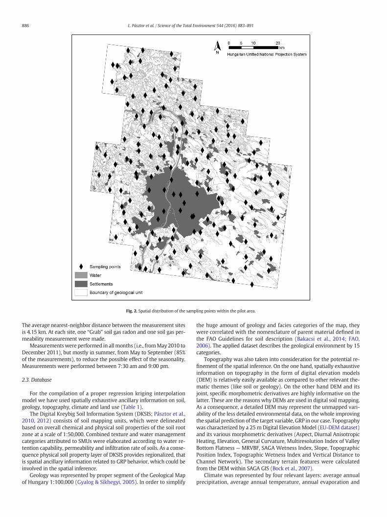
Fig. 2. Spatial distribution of the sampling points within the pilot area.

886 L. Pásztor et al. / Science of the Total Environment 544 (2016) 883–891

The average nearest-neighbor distance between themeasurement sitesis 4.15 km. At each site, one “Grab” soil gas radon and one soil gas per-meability measurement were made.

Measurementswere performed in allmonths (i.e., fromMay2010 toDecember 2011), but mostly in summer, from May to September (85%of the measurements), to reduce the possible effect of the seasonality.Measurements were performed between 7:30 am and 9:00 pm.

2.3. Database

For the compilation of a proper regression kriging interpolationmodel we have used spatially exhaustive ancillary information on soil,geology, topography, climate and land use (Table 1).

The Digital Kreybig Soil Information System (DKSIS; Pásztor et al.,2010, 2012) consists of soil mapping units, which were delineatedbased on overall chemical and physical soil properties of the soil rootzone at a scale of 1:50,000. Combined texture and water managementcategories attributed to SMUs were elaborated according to water re-tention capability, permeability and infiltration rate of soils. As a conse-quence physical soil property layer of DKSIS provides regionalized, thatis spatial ancillary information related to GRP behavior, which could beinvolved in the spatial inference.

Geology was represented by proper segment of the Geological Mapof Hungary 1:100,000 (Gyalog & Síkhegyi, 2005). In order to simplify

the huge amount of geology and facies categories of the map, theywere correlated with the nomenclature of parent material defined inthe FAO Guidelines for soil description (Bakacsi et al., 2014; FAO,2006). The applied dataset describes the geological environment by 15categories.

Topography was also taken into consideration for the potential re-finement of the spatial inference. On the one hand, spatially exhaustiveinformation on topography in the form of digital elevation models(DEM) is relatively easily available as compared to other relevant the-matic themes (like soil or geology). On the other hand DEM and itsjoint, specific morphometric derivatives are highly informative on thelatter. These are the reasons why DEMs are used in digital soil mapping.As a consequence, a detailed DEM may represent the unmapped vari-ability of the less detailed environmental data, on the whole improvingthe spatial prediction of the target variable, GRP in our case. Topographywas characterized by a 25 m Digital Elevation Model (EU-DEM dataset)and its various morphometric derivatives (Aspect, Diurnal AnisotropicHeating, Elevation, General Curvature, Multiresolution Index of ValleyBottom Flatness — MRVBF, SAGA Wetness Index, Slope, TopographicPosition Index, Topographic Wetness Index and Vertical Distance toChannel Network). The secondary terrain features were calculatedfrom the DEM within SAGA GIS (Bock et al., 2007).

Climate was represented by four relevant layers: average annualprecipitation, average annual temperature, annual evaporation and

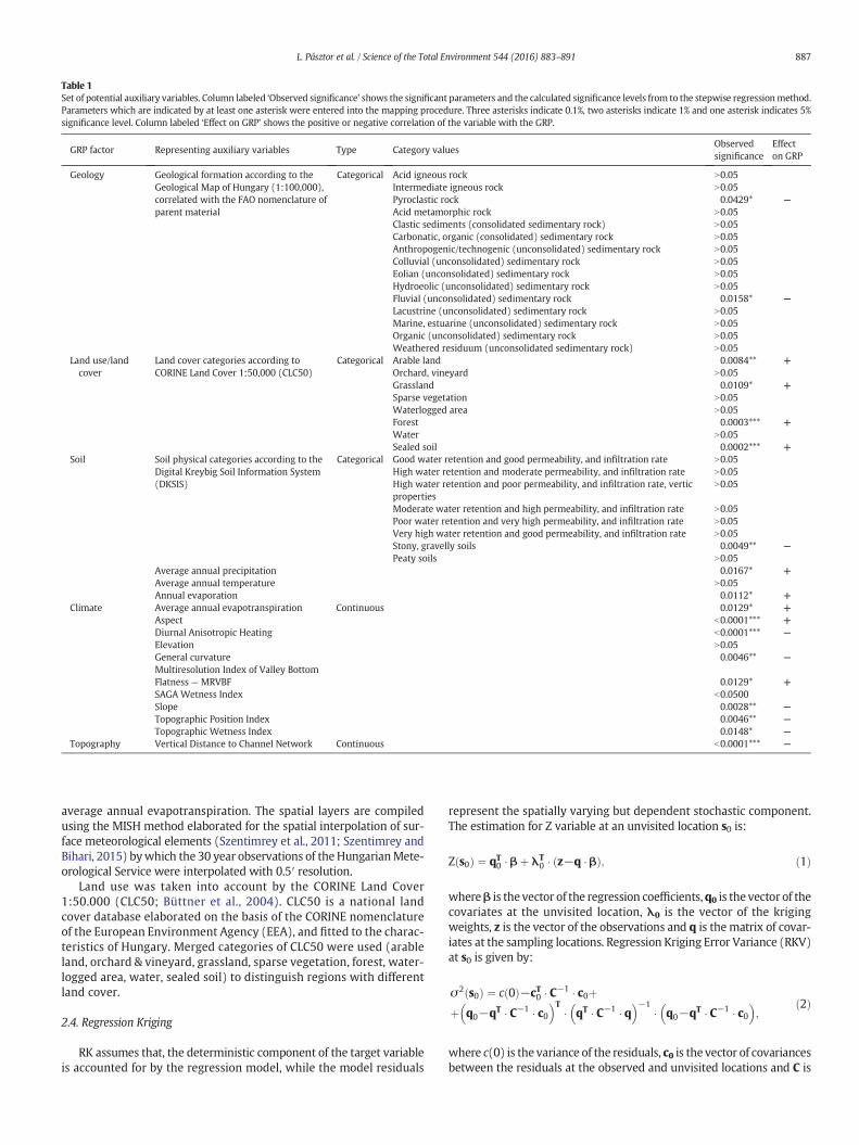
Table 1Set of potential auxiliary variables. Column labeled ‘Observed significance’ shows the significant parameters and the calculated significance levels from to the stepwise regressionmethod.Parameters which are indicated by at least one asterisk were entered into the mapping procedure. Three asterisks indicate 0.1%, two asterisks indicate 1% and one asterisk indicates 5%significance level. Column labeled ‘Effect on GRP’ shows the positive or negative correlation of the variable with the GRP.

GRP factor Representing auxiliary variables Type Category valuesObservedsignificance

Effecton GRP

Geology Geological formation according to theGeological Map of Hungary (1:100,000),correlated with the FAO nomenclature ofparent material

Categorical Acid igneous rock N0.05Intermediate igneous rock N0.05Pyroclastic rock 0.0429* −Acid metamorphic rock N0.05Clastic sediments (consolidated sedimentary rock) N0.05Carbonatic, organic (consolidated) sedimentary rock N0.05Anthropogenic/technogenic (unconsolidated) sedimentary rock N0.05Colluvial (unconsolidated) sedimentary rock N0.05Eolian (unconsolidated) sedimentary rock N0.05Hydroeolic (unconsolidated) sedimentary rock N0.05Fluvial (unconsolidated) sedimentary rock 0.0158* −Lacustrine (unconsolidated) sedimentary rock N0.05Marine, estuarine (unconsolidated) sedimentary rock N0.05Organic (unconsolidated) sedimentary rock N0.05Weathered residuum (unconsolidated sedimentary rock) N0.05

Land use/landcover

Land cover categories according toCORINE Land Cover 1:50,000 (CLC50)

Categorical Arable land 0.0084** +Orchard, vineyard N0.05Grassland 0.0109* +Sparse vegetation N0.05Waterlogged area N0.05Forest 0.0003*** +Water N0.05Sealed soil 0.0002*** +

Soil Soil physical categories according to theDigital Kreybig Soil Information System(DKSIS)

Categorical Good water retention and good permeability, and infiltration rate N0.05High water retention and moderate permeability, and infiltration rate N0.05High water retention and poor permeability, and infiltration rate, verticproperties

N0.05

Moderate water retention and high permeability, and infiltration rate N0.05Poor water retention and very high permeability, and infiltration rate N0.05Very high water retention and good permeability, and infiltration rate N0.05Stony, gravelly soils 0.0049** −Peaty soils N0.05

Climate

Average annual precipitation

Continuous

0.0167* +Average annual temperature N0.05Annual evaporation 0.0112* +Average annual evapotranspiration 0.0129* +

Topography

Aspect

Continuous

b0.0001*** +Diurnal Anisotropic Heating b0.0001*** −Elevation N0.05General curvature 0.0046** −Multiresolution Index of Valley BottomFlatness — MRVBF 0.0129* +SAGA Wetness Index b0.0500Slope 0.0028** −Topographic Position Index 0.0046** −Topographic Wetness Index 0.0148* −Vertical Distance to Channel Network b0.0001*** −

887L. Pásztor et al. / Science of the Total Environment 544 (2016) 883–891

average annual evapotranspiration. The spatial layers are compiledusing the MISH method elaborated for the spatial interpolation of sur-face meteorological elements (Szentimrey et al., 2011; Szentimrey andBihari, 2015) bywhich the 30 year observations of theHungarianMete-orological Service were interpolated with 0.5′ resolution.

Land use was taken into account by the CORINE Land Cover1:50.000 (CLC50; Büttner et al., 2004). CLC50 is a national landcover database elaborated on the basis of the CORINE nomenclatureof the European Environment Agency (EEA), and fitted to the charac-teristics of Hungary. Merged categories of CLC50 were used (arableland, orchard & vineyard, grassland, sparse vegetation, forest, water-logged area, water, sealed soil) to distinguish regions with differentland cover.

2.4. Regression Kriging

RK assumes that, the deterministic component of the target variableis accounted for by the regression model, while the model residuals

represent the spatially varying but dependent stochastic component.The estimation for Z variable at an unvisited location s0 is:

Z s0ð Þ ¼ qT0 � βþ λT

0 � z−q � βð Þ; ð1Þ

whereβ is the vector of the regression coefficients,q0 is the vector of thecovariates at the unvisited location, λ0 is the vector of the krigingweights, z is the vector of the observations and q is the matrix of covar-iates at the sampling locations. Regression Kriging Error Variance (RKV)at s0 is given by:

σ2 s0ð Þ ¼ c 0ð Þ−cT0 � C−1 � c0þþ q0−qT � C−1 � c0� �T

� qT � C−1 � q� �−1

� q0−qT � C−1 � c0� �

;ð2Þ

where c(0) is the variance of the residuals, c0 is the vector of covariancesbetween the residuals at the observed and unvisited locations and C is

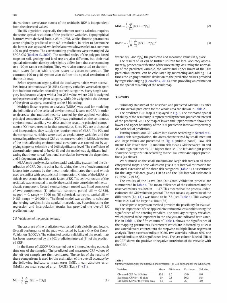
Table 2Summary statistics for the observed and predicted 145 GRP sites and for the whole area.

Variable Mean Minimum Maximum Std. dev.

Observed GRP for 145 sites 10.8 1.0 43.9 8.6Estimated GRP for 145 sites 9.4 0.8 36.2 5.5Estimated GRP for the whole area 8.6 0.2 75 4.9

888 L. Pásztor et al. / Science of the Total Environment 544 (2016) 883–891

the variance–covariance matrix of the residuals. RKV is independentfrom the observed values.

The RK algorithm, especially the inherent matrix calculus, requiresthe same spatial resolution of the predictor variables. Topographicalfeatures were derived from a 25 m DEM, while climatic parameterswere originally predicted with 0.5′ resolution. In order to harmonizethe former was upscaled, while the latter was downscaled to a common100 m grid system. The corresponding predictors were resampled viaSAGA GIS (Bock et al., 2007). The nominal scales of the polygon-basedmaps on soil, geology and land use are also different, but their realspatial information density only slightly differs from that correspondingto a 100 m raster resolution. They were also converted to the com-mon raster format with proper raster-to-vector conversion. Thecommon 100 m grid system also defines the spatial resolution ofthe result map.

Before regression kriging, all of the auxiliary variables were normal-ized into a common scale (0–255). Category variables were taken apartinto indicator variables according to their categories. Every single cate-gory has become a layer with a 0 or 255 value, where 255 is assignedto the presence of the given category, while 0 is assigned to the absenceof the given category, according to the 8 bit coding.

Multiple linear regression analysis (MLRA) was used for modelingthe joint effect of the selected environmental factors on GRP. In orderto decrease the multicollinearity carried by the applied variablesprincipal component analysis (PCA) was performed on the continuousenvironmental auxiliary variables and the resulting principal compo-nents (PCs) were used in further procedures. Since PCs are orthogonaland independent, they satisfy the requirements of MLRA. The PCs andthe categorical variables were used as explanatory variables and thenatural logarithm values of GRP as response variable in MLRA. Selectionof the most affecting environmental covariates was carried out by ap-plying stepwise selection and 0.05 significance level. The coefficient ofdetermination proved to be 0.41% and the model was significant, indi-cating that there is real functional correlation between the dependentand independent variables.

MLRA only partly explains the spatial variability (pattern) of the dis-tribution of GRP. On the other hand, taking the role of environmentalfactors into account by the linear model eliminates the trend whichused to conflictwith geostatistical interpolation. Kriging of theMLRA re-siduals represents the stochastic factor of RK. The semivariogram of theresiduals was estimated tomodel the spatial auto-correlation of the sto-chastic component. Nested semivariogram model was fitted composedof two components: (i) spherical, isotropic, partial sill = 0.1836,nugget = 0, range = 3000 m; (ii) spherical, isotropic, partial sill =0.185, range = 24,000 m. The fitted model was applied to calculatethe kriging weights in the spatial interpolation. Superimposing theregression and interpolation results has provided the overall RKprediction map.

2.5. Validation of the prediction map

The accuracy of the prediction was tested both globally and locally.Overall performance of the map was tested by Leave-One-Out Cross-Validation (LOOCV). The estimated spatial reliability of the result maphas been represented by the 90% prediction interval (PI) of the predict-ed GRP.

In the frame of LOOCV RK is carried out n-1 times, leaving out eachtime one of the samples. The predicted and measured GRP values ofthe left-out sample are then compared. The series of the results ofthese comparisons is used for the estimation of the overall accuracy bythe following indicators: mean error (ME), mean absolute error(MAE), root mean squared error (RMSE) (Eqs. (1)–(3)).

ME ¼ 1n∙∑

n

i¼1z sið Þ � z sið Þ½ � ð1Þ

MAE ¼ 1n∙∑

n

i¼1z sið Þ � z sið Þj j ð2Þ

RMSE ¼ffiffiffiffiffiffiffiffiffiffiffiffiffiffiffiffiffiffiffiffiffiffiffiffiffiffiffiffiffiffiffiffiffiffiffiffiffiffiffiffiffiffi1n∙∑

n

i¼1z sið Þ � z sið Þ½ �2

sð3Þ

where zðsiÞ and z(si) the predicted and measured values in si place.The results of RK can be further utilized for local accuracy assess-

ment by proper quantification of the uncertainty. Assuming the normal-ity of the predicted variable, the lower and upper limits of the 90%prediction interval can be calculated by subtracting and adding 1.64times the kriging standard deviation to the prediction values providedby regression kriging (Heuvelink, 2014), thus providing an estimationfor the spatial reliability of the result map.

3. Results

Summary statistics of the observed and predicted GRP for 145 sitesand the overall prediction for the whole area are shown in Table 2.

The predicted GRP map is displayed in Fig. 3. The estimated spatialreliability of the resultmap is represented by the 90% prediction intervalof the predicted GRP. The map of lower and upper estimate shows thelower and upper boundary of the 90% prediction interval respectivelyfor each cell of prediction.

Turning continuousGRP values into classes according toNeznal et al.(2004) risk categorization, the areas characterized by small, mediumand large values are presented in Fig. 4 (middle panel). Low riskmeans GRP lower than 10, medium risk means GRP between 10 and35 and high risk means GRP higher than 35. The left and right panelsshow the categorization according to the 90% lower and upper predic-tions (as above).

We summed up the small, medium and large risk areas on all threecategorized maps. These values can give a 90% interval estimation forthe areal extension of the three risk categories (Table 3). Our estimatefor the large risk area gave 1110 ha and the 90% interval estimate is(719 ha, 1749 ha).

The results of the Leave-One-Out-Cross-Validation process aresummarized in Table 4. The mean difference of the estimated and theobserved values resulted in −1.47. This means that the process under-estimates the GRP values in general. The root means square value of thedifferences (Eq. (3)) was found to be 7.5 (see Table 4). This averagevalue is 21% of the large risk limit (35).

The stepwise regressionmethod provides the possibility for evaluat-ing the importance of the applied environmental covariables using thesignificance of the entering variables. The auxiliary category variables,which proved to be important in the analysis are indicated with aster-isks in Table 1. The fifth column of Table 1. shows the significance ofthe mapping parameters. Parameters which are indicated by at leastone asterisk were entered into the stepwise multiple linear regressionanalysis. Three asterisks indicate 99.9%, two asterisks indicate 99%, oneasterisk indicates 95% significance level. The last column labeled ‘Effecton GRP’ shows the positive or negative correlation of the variable withthe GRP.

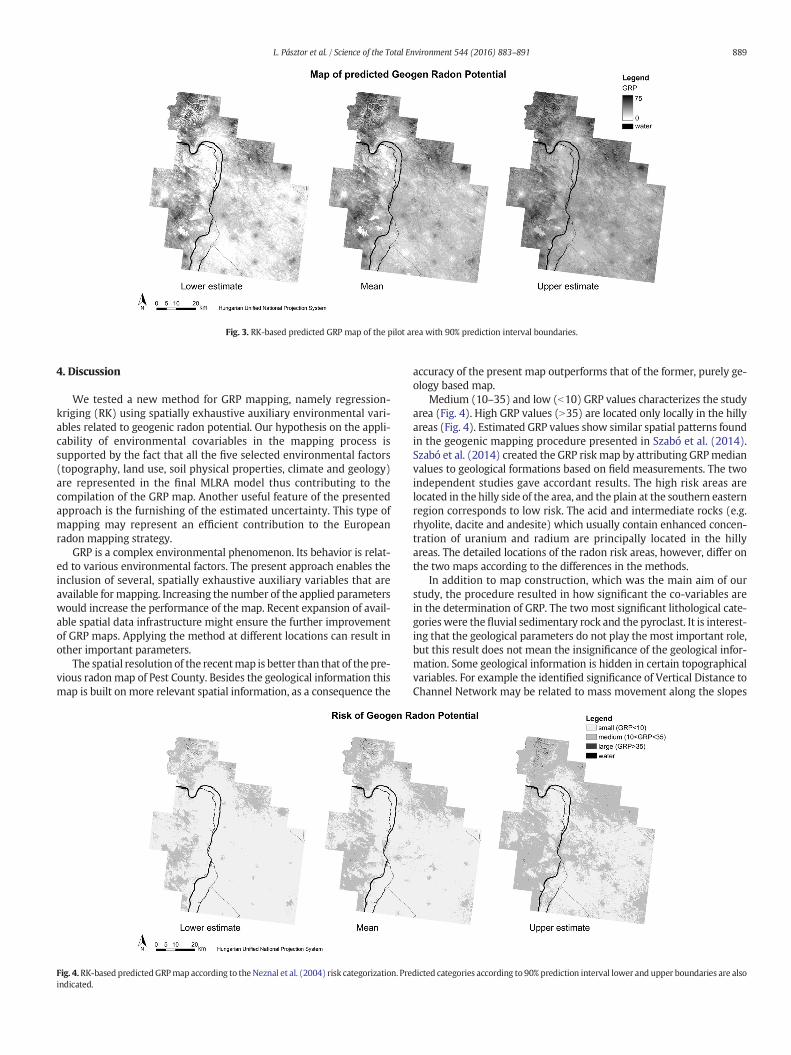
Fig. 3. RK-based predicted GRP map of the pilot area with 90% prediction interval boundaries.

889L. Pásztor et al. / Science of the Total Environment 544 (2016) 883–891

4. Discussion

We tested a new method for GRP mapping, namely regression-kriging (RK) using spatially exhaustive auxiliary environmental vari-ables related to geogenic radon potential. Our hypothesis on the appli-cability of environmental covariables in the mapping process issupported by the fact that all the five selected environmental factors(topography, land use, soil physical properties, climate and geology)are represented in the final MLRA model thus contributing to thecompilation of the GRP map. Another useful feature of the presentedapproach is the furnishing of the estimated uncertainty. This type ofmapping may represent an efficient contribution to the Europeanradon mapping strategy.

GRP is a complex environmental phenomenon. Its behavior is relat-ed to various environmental factors. The present approach enables theinclusion of several, spatially exhaustive auxiliary variables that areavailable for mapping. Increasing the number of the applied parameterswould increase the performance of the map. Recent expansion of avail-able spatial data infrastructure might ensure the further improvementof GRP maps. Applying the method at different locations can result inother important parameters.

The spatial resolution of the recentmap is better than that of thepre-vious radonmap of Pest County. Besides the geological information thismap is built on more relevant spatial information, as a consequence the

Fig. 4.RK-based predictedGRPmap according to the Neznal et al. (2004) risk categorization. Preindicated.

accuracy of the present map outperforms that of the former, purely ge-ology based map.

Medium (10–35) and low (b10) GRP values characterizes the studyarea (Fig. 4). High GRP values (N35) are located only locally in the hillyareas (Fig. 4). Estimated GRP values show similar spatial patterns foundin the geogenic mapping procedure presented in Szabó et al. (2014).Szabó et al. (2014) created the GRP risk map by attributing GRPmedianvalues to geological formations based on field measurements. The twoindependent studies gave accordant results. The high risk areas arelocated in the hilly side of the area, and the plain at the southern easternregion corresponds to low risk. The acid and intermediate rocks (e.g.rhyolite, dacite and andesite) which usually contain enhanced concen-tration of uranium and radium are principally located in the hillyareas. The detailed locations of the radon risk areas, however, differ onthe two maps according to the differences in the methods.

In addition to map construction, which was the main aim of ourstudy, the procedure resulted in how significant the co-variables arein the determination of GRP. The two most significant lithological cate-gorieswere the fluvial sedimentary rock and the pyroclast. It is interest-ing that the geological parameters do not play the most important role,but this result does not mean the insignificance of the geological infor-mation. Some geological information is hidden in certain topographicalvariables. For example the identified significance of Vertical Distance toChannel Network may be related to mass movement along the slopes

dicted categories according to 90% prediction interval lower and upper boundaries are also

Table 390% interval estimate for the areal extension of the three GRP risk categories.

GRP risk categoryArea affected [ha]

Lower estimate Mean estimate Upper estimate

Small 444,529 383,087 265,974Medium 82,626 143,677 260,151Large 719 1110 1749

Table 4Result of the Leave-One-Out-Cross-Validation(LOOCV). (ME=mean error, MAE=mean ab-solute error, RMSE = root mean squared error,AVRD = average Value of the relativedifference).

ME −1.47MAE 5.42RMSE 7.50

890 L. Pásztor et al. / Science of the Total Environment 544 (2016) 883–891

mixing on-site origin and transportedmaterial. More generally the ero-sion on the hilly/mountainous areas as well as the deposition on theplains is partly driven by topography, while they determine some geo-logical and pedological features like thickness of soil – that is distanceto bedrock – which can have significant effects on GRP. The emanationcoefficient of soils can also be affected by diurnal asymmetric heatingon slopes with differing aspect. Land use properties also have signifi-cance in radon risk. This could be attributed to their effect on the perme-ability of soils similarly to that of soil physical categories.

A further improvement of the RK-based GRP mapping would un-doubtedly be the introduction of scanned images provided by airbornegammameasurements. The gamma activity reflects the potassium, ura-nium or the thorium content of the soil in the first 30 cm from the sur-face. One of these, the uranium concentration, is amain factor in the soilair radon concentration, the main factor of geogenic radon potential.

5. Conclusions

We investigated a new approach (regression kriging) for mappinggeogenic radon potential, which has several advantages such as applica-tion of environmental co-variables (used in spatially continuous form),refined spatial resolution and inherent accuracy assessment. Our resultsdemonstrated that not only pure geological information should be re-lied on in GRP mapping, but further environmental variables (relatedto climate, land use, soil and topography) also play important roles.The resultingmap is characterized by global and localmeasures of its ac-curacy. The method also provides interval estimation for the spatial ex-tension of the areas of risk categories. All of these outputs provide usefulcontribution to spatial planning, radon action planning and decisionmaking.

Acknowledgements

Our work has been partly supported by the Hungarian NationalScientific Research Foundation (OTKA, Grant No. K105167 and OTKA,Grant No. PD115810). Special thanks go to Csaba Szabó, LithosphereFluid Research Lab (LRG), for his valuable support.

References

Bakacsi, Zs., Laborczi, A., Szabó, J., Takács, K., Pasztor, L. (2014). Proposed correlation be-tween the legend of the 1:100,000 scale geological map and the FAO code systemfor soil parent material. (in Hungarian) Agrokémia és Talajtan 63(2), 189–202.

Bock, M., Böhner, J., Conrad, O., Köthe, R., Ringeler, A., 2007. Methods for creating func-tional soil databases and applying Digital Soil Mapping with SAGA GIS. In: Hengl, T.,Panagos, P., Jones, A., Toth, G. (Eds.), Status and Prospect of Soil Information inSouth-eastern Europe: Soil Databases, Projects and ApplicationsEUR 22646 EN

Scientific and Technical Research series. Office for Official Publications of theEuropean Communities, Luxemburg, pp. 149–162.

Bossew, P., 2014. Determination of radon prone areas by optimized binary classification.J. Environ. Radioact. 129 (2014), 121–132.

Bossew, P., Tollefsen, T., Gruber, V., De Cort, M., 2013. The European radon mapping pro-ject. IX. Latin American IRPA Regional Congress on Radiation Protection and Safety—IRPA 2013. Sociedade Brasileira De Protecao Radiologica - SBPR, Rio de Janeiro, Brazil(April 15–19, 2013).

Buttafuoco, G., Tallarico, A., Falcone, G., 2007. Mapping soil gas radon concentration: acomparative study of geostatistical methods. Environ. Monit. Assess. 131, 135–151.

Büttner, Gy., Maucha, G., Bíró, M., Kosztra, B., Pataki, R., Petrik, O. (2004). National landcover database at scale 1:50,000 in Hungary. EARSeL eProceedings, 3(3), 323–330.

Darby, S., Hill, D., Auvinen, A., Barrios-Dios, J.M., Baysson, H., Bochicchio, F., Deo, H., Falk,R., Forastiere, F., Hakama, M., Heid, I., Kreienbrock, L., Kreuzer, M., Lagarde, F.,Makelainen, I., Muirgead, C., Oberaigner, W., Pershagen, G., Ruani-Ravina, A.,Ruosteenoja, E., Rosario, A.S., Tirmarche, M., Tomasek, L., Whitley, E., Wichmann,H.E., Doll, R., 2005. Radon in homes and risk of lung cancer: collaborative analysisof individual data from 13 European case–control studies. Br. Med. J. 330 (7485),223–226.

Dubois, G., Bossew, P., Tollefsen, T., De Cort, M., 2010. First steps towards a European atlasof natural radiation: status of the European indoor radon map. J. Environ. Radioact.101, 786–798.

Durridge Company Inc., 2000. RAD7 electronic radon detector, User Manual.EU-DEM dataset. http://www.eea.europa.eu/data-and-maps/data/eu-dem#tab-european-

data European Environment Agency.Faheem, M., Matiullah, 2008. Radon exhalation and its dependence on moisture content

from samples of soil and building materials. Radiat. Meas. 43, 1458–1462.FAO, 2006. Guidelines for soil description. fourth ed. p. 97 (Rome, FAO).Friedmann, H., 2005. Final results of the Austrian radon project. Health Phys. 89 (4),

339–348.Gessler, P.E., Moore, I.D., McKenzie, N.J., Ryan, P.J., 1995. Soil–landscape modelling and

spatial prediction of soil attributes. Int. J. Geogr. Inf. Syst. 9, 421–432.Gue, L., 2015. David Suzuki Foundation Report: Revisiting Canada's Radon Guideline

(ISBN digital: 978–1-897375-91-4 print: 978–1-897375-90-7).Gyalog, L., Síkhegyi, F. (Eds.), 2005. Geological Map of Hungary, 1:100 000. Geological In-

stitute of Hungary, Budapest (In Hungarian). Digital version. Retrieved December, 1,2008 from http://loczy.mfgi.hu/fdt100/.

Hengl, T., Heuvelink, G.M.B., Stein, A., 2004. A generic framework for spatial prediction ofsoil variables based on regression-kriging. Geoderma 122 (1-2), 75–93.

Hengl, T., 2009. A practical guide to geostatistical mapping. University of Amsterdam,Amsterdam.

Heuvelink, G.B.M., 2014. Uncertainty quantification of GlobalSoilMap products. In:Arrouays, et al. (Eds.), GlobalSoilMap. Taylor & Francis Group, London,pp. 335–340.

Ielsch, G., Ferry, C., Tymen, G., Robé, M.C., 2002. Study of a predictive methodology forquantification and mapping of the radon-222 exhalation rate. J. Environ. Radioact.63 (1), 15–33.

Kemski, J., Siehl, A., Stegemann, R., Valdivia-Manchego, M., 2001. Mapping the geogenicradon potential in Germany. Sci. Total Environ. 272, 217–230.

Koorevaar, P., Menelik, G., Dirksen, C., 1983. Elements of Soil Physics. Developments inSoil Science vol. 13. Elsevier, Amsterdam, New York.

McKenzie, N.J., Ryan, P.J., 1999. Spatial prediction of soil properties using environmentalcorrelation. Geoderma 89, 67–94.

Neznal, M., Neznal, M., Matolin, M., Barnet, I., Miksova, J., 2004. The New Method forAssessing the Radon Risk of Building Sites. Czech Geol. Survey Special Papers vol.16. Czech Geol. Survey, Prague (http://www.radon-vos.cz/pdf/metodika.pdf).

Oliver, M.A., Khayrat, A.L., 2001. A geostatistical investigation of the spatial variation ofradon in soil. Comput. Geosci. 27, 939–957.

Pásztor, L., Szabó, J., Bakacsi, Z., 2010. Digital processing and upgrading of legacy data col-lected during the 1:25.000 scale kreybig soil survey. Acta Geodaet. Geophys. Hung.45, 127–136.

Pásztor, L., Szabó, J., Bakacsi, Zs., Matus, J. & Laborczi, A. 2012. Compilation of 1:50,000scale digital soil maps for Hungary based on the digital kreybig soil informationsystem. J. Maps 8(3): 215–219.

Sakoda, A., Ishimori, Y., Hanamoto, K., Kataoka, T., Kawabe, A., Yamaoka, K., 2010.Experimental and modeling studies of grain size and moisture content effects onradon emanation. Radiat. Meas. 45, 204–210.

Scull, P., Franklin, J., Chadwick, O.A., McArthur, D., 2003. Predictive soil mapping: a review.Progress in Physical Geography 27, 171–197.

Schumann, R., Gundersen, L.C.S., 1996. Geologic and climatic controls on the radonemanation coefficient. Environ. Int. 22 (Suppl. I), S439–S446.

Schweikani, R., Giaddui, T.G., Durrani, S.A., 1995. The effect of soil parameters on theradon concentration values in the environment. Radiat. Meas. 25 (1-4), 581–584.

Sun, K., Guo, Q., Cheng, J., 2004. The effect of some soil characteristics on soil radon con-centration and radon exhalation from soil surface. J. Nucl. Sci. Technol. 41 (11),1113–1117.

Szabó, K.Z., Jordan, G., Horváth, Á., Szabó, C., 2014. Mapping the geogenic radon potential:methodology and spatial analysis for central Hungary. J. Environ. Radioact. 129,107–120.

Szentimrey, T., Bihari, Z., 2015. Meteorological Interpolation based on Surface Homoge-nized Data Basis (MISH v1.02). Hungarian Meteorological Service (http://www.dmcsee.org/uploads/file/330_1_mishmanual.pdf p.33).

Szentimrey, T., Bihari, Z., Lakatos, M., Szalai, S., 2011. Mathematical, methodological ques-tions concerning the spatial interpolation of climate elements. Proceedings from theSecond Conference on Spatial Interpolation in Climatology and Meteorology, Buda-pest, Hungary, 2009. Időjárás 115, pp. 1-2–1-11.

891L. Pásztor et al. / Science of the Total Environment 544 (2016) 883–891

Tanner, A.B., 1980. Radon migration in the ground: supplementary review. In: Gesell,T.F., Lowder, W.M. (Eds.), Proc. Natural Radiation Environment III, Conf-780422.US Dept. of Commerce, National Technical Information Service, Springfield, VA,p. 5 (1980).

Tollefsen, T., Gruber, V., Bossew, P., De Cort, M., 2011. Status of the European indoor radonmap. Radiat. Prot. Dosim. 145, 110–116.

UNSCEAR, 2008. Effects of Ionizing Radiation. Vol. I. Annex B. United Nations, New York.Winkler, R., Ruckerbauer, F., Bunzl, K., 2001. Radon concentration in soil gas: a compari-

son of the variability resulting from different methods, spatial heterogeneity andseasonal fluctuations. Sci. Total Environ. 272, 273–282.