Schwarz Waveform Relaxation Method for the

Viscous Shallow Water Equations

Veronique Martin

LAGA Universite Paris XIIImartin@math.univ-paris13.fr

Summary. We are interested in solving time dependent problems using domaindecomposition method. In the classical methods, one discretizes first the time di-mension and then one solves a sequence of steady problems by a domain decom-position method. In this paper, we study a Schwarz Waveform Relaxation methodwhich treats directly the time dependent problem. We propose algorithms for theviscous Shallow Water equations.

1 Introduction

The principle of domain decomposition methods is to partition the initial do-main into several subdomains and then to use a processor per subdomain tosolve the equation. The global solution is obtained if the processors exchangeinformations in an iterative way at the common interfaces. This method is use-ful to solve problems with a great number of unknowns. And it is more andmore used to simulate complex phenomena with different spatial discretiza-tions in each subdomain.Solving time dependent problems, classical methods discretize the time dimen-sion first and then use domain decomposition methods on the steady problemsat each time step. Different strategies rely on the choice of transmission con-ditions (see Schwarz [1870], Lions [1990], Quarteroni and Valli [1999], Japhetet al. [2001]). In particular, in Japhet et al. [2001] transmission conditionsare designed which minimize the convergence rate. This strategy proved tobe very useful for many steady problems, for instance convection diffusion,Euler or Helmholtz equations. However the classical strategy to treat evolu-tion equations does not allow to manage different time discretizations for eachsubdomain.In some recent works a domain decomposition method for evolution prob-lems quite different from the classical one has been proposed: they applythe iterative algorithm directly to the time dependent problem. This SchwarzWaveform Relaxation (SWR) method, permits to work with different time dis-cretizations in each subdomain and therefore it provides an accurate method

654 Veronique Martin

to simulate complex phenomena. This method is a derivation of the WaveformRelaxation method: inspired by the Picard iteration, it has been studied inLelarasmee et al. [1982] for integrated circuit simulation and its convergencecan be accelerated by a multigrid method (see Vandewalle [1993]).The first SWR algorithm used Dirichlet conditions on the interfaces (see Gan-der and Zhao [1997], Gander and Stuart [1998]) and more recently more ap-propriate interface conditions have been written in Gander et al. [1999]. Inthis paper we apply Schwarz Waveform Relaxation methods to the ShallowWater equations.

The Shallow Water equations are obtained by average of the Navier-Stokesequations when the depth of the water is much smaller than the other dimen-sions of the basin. If linearized around the velocity field U = 0 this modelbecomes (see for example Pedlosky [1987])

∂tU − νU + DU + c2∇h = τs/ρ0,∂th + divU = 0.

(1)

where U = (u, v) is the velocity field, h the depth of the water, D =

(

0 −ff 0

)

,

c2 is the speed of internal gravity waves, ν the viscosity of the fluid, τs isthe wind stress and f the Coriolis force supposed to be constant for thetheory. We introduce the Shallow Water operator LSW where W = (U, h)and we are interested in solving LSWW = FW in Ω × (0, T ) with T < +∞,W(·, ·, 0) = W0 in Ω and with boundary conditions.

In this paper we study Schwarz Waveform Relaxation algorithms to solvethe Shallow Water equations. We work on the space R

2 which is split into twohalf spaces Ω− = (−∞, L) × R and Ω+ = (0, +∞) × R, L ≥ 0 is the overlapand let Γ0 = y ∈ R, x = 0 and ΓL = y ∈ R, x = L denote the interfaces.

In Section 2 we propose an algorithm with Dirichlet interface conditions(which needs an overlap), then we propose in Section 3 an optimized algorithmwhich can be implemented without overlap. Finally we show numerical resultswhich underline the efficiency of the optimized method (Sec. 4). More detailsabout theorems will be found in Martin [2003].

2 Classical Schwarz Waveform Relaxation Method

Following ideas introduced in Gander and Zhao [1997] for the heat equation,we propose the following algorithm for L > 0

LSW Wk+1− = FW in Ω− × (0, T ),

Wk+1− (·, ·, 0) = W0 in Ω−,

Uk+1− = Uk

+ on ΓL × (0, T ),

LSW Wk+1+ = FW in Ω+ × (0, T ),

Wk+1+ (·, ·, 0) = W0 in Ω+,

Uk+1+ = Uk

− on Γ0 × (0, T ),

(2)

where FW = (F1, F2, 0) = (F, 0), W0 = (U0, h0) and k ≥ 0. This algorithmis initialized by U0

± in H2,1(Ω± × (0, T )) such that U0±(·, ·, 0) = U0 in Ω±.

SWR Method for SW equations 655

We recall that we can find in Lions and Magenes [1972] the definition ofanisotropic Sobolev spaces and a theorem of extension. If we use moreover aFourier transform in y, a Laplace transform in t and a priori estimates, thenwe can prove that algorithm (2) is well posed.

Theorem 1. Let F be in L2(0, T ;L2(Ω)), W0 = (U0, h0) in H1(Ω)×H1(Ω).The algorithm (2) defines two unique sequences Wk

± = (Uk±, hk

±) in H2,1(Ω±×(0, T )) × H1,1(Ω± × (0, T )) with ∇h± in H1(0, T ;L2(Ω±)).

We can prove that algorithm (2) converges by computing its convergence ratewritten in Fourier-Laplace variables.

Theorem 2. Let F be in L2(0, T ;L2(Ω)), W0 = (U0, h0) in H1(Ω)×H1(Ω).The algorithm (2) converges in L2(0, T ;H1(Ω±)) × L2(0, T ; L2(Ω±)).

It is well-known that this algorithm is not efficient: the overlap between thetwo subdomains is necessary and the convergence is slow. In Gander et al.[1999] interface conditions have been introduced which are more appropriate.In the next section we apply this new strategy to the Shallow Water equations.

3 Optimized Schwarz Waveform Relaxation Method

In this section we consider the case without overlap of the subdomains (L = 0)and we denote by Γ the common interface. Since physical transmission con-ditions, (i.e. quantities that must be continuous through the interface) are U

and −ν∂xU + c2(h, 0)t we propose the algorithm

8

<

:

LSW Wk+1

−

= FW in Ω−× (0, T )

Wk+1

−

(·, ·, 0) = W0 in Ω−

−ν∂xUk+1

−

+ c2(hk+1

−

, 0)t− Λ+Uk+1

−

= −ν∂xUk

+ + c2(hk

+, 0)t− Λ+Uk

+ on Γ × (0, T )

8

<

:

LSW Wk+1

+ = FW in Ω+ × (0, T )

Wk+1

+ (·, ·, 0) = W0 in Ω+

ν∂xUk+1

+ − c2(hk+1

+ , 0)t− Λ−Uk+1

+ = ν∂xUk

−− c2(hk

−, 0)t

− Λ−Uk

−on Γ × (0, T )

(3)with Λ+ and Λ− to be defined. The next theorem shows that we can choosethe operators Λ± in an optimal way.

Theorem 3. The operators Λ± can be chosen such that algorithm (3) con-verges in two iterations. These operators are denoted Λ±

exac.

These transmission conditions coincide with absorbing boundary conditions(see for example Gander et al. [1999] for time dependent scalar equations). Asfor many problems the operators Λ±

exac are not differential and difficult to use,therefore we have to approximate them (see for example Nataf and Rogier[1995]). For low spatial frequencies, small Coriolis force and small viscosityΛ±

exac are approximated by:

656 Veronique Martin

Λ±

app =

(

c + ν2c

∂t 00 p

)

,

with p a constant to be chosen. The following theorem gives a result of well-posedness for the corresponding algorithm. It can be proved by a Fourier-Laplace analysis and by an extension theorem.

Theorem 4. Let F be in H2,1(Ω×(0, T )), W0 = (U0, h0) in H3(Ω)×H3(Ω)and p be a strictly positive constant. If algorithm (3) is initialized by U0

±

in H4,2(Ω± × (0, T )) and h0± in H1(0, T ; H3(Ω±)) with some compatibil-

ity relations satisfied at t = 0, then algorithm (3) defines two unique se-quences (Uk

±, hk±) in H4,2(Ω± × (0, T )) × H3,2(Ω± × (0, T )) with hk

± inH1(0, T ; H3(Ω±)).

By a priori estimates we can prove that algorithm (3) converges.

Theorem 5. Let F be in H2,1(Ω×(0, T )), W0 = (U0, h0) in H3(Ω)×H3(Ω)and p be a strictly positive constant. If algorithm (3) is initialized by U0

±

in H4,2(Ω± × (0, T )) and h0± in H1(0, T ; H3(Ω±)) with some compatibility

relations satisfied at t = 0, then the sequences (Uk+1± , hk+1

± ) defined by (3)converge in L2(0, T ;H1(Ω±)) × L2(0, T ; L2(Ω±)).

4 Numerical Results

4.1 Description of the experience

We work on a rectangular basin with closed boundaries, which extends from0 to 15000 km in the x (east-west) direction and from -1500 km to 1500 kmin the y (north-south) direction. The wind stress τ s = (τx, τy) is purely zonal(τy = 0) and we have τx = 0.5τ0(1 + tanh((x − x0)/L)), with τ0 = 5 · 10−2

N/m2 and x0 = 3000 km. The value of the physical parameters are c = 3m/s and ν = 500 m2/s. For further details about the experience the readeris referred to Jensen and Kopriva [1990].

The Figure 1 shows the evolution in time of the depth of water. At t = 0 theocean is at rest when the wind stress begins to be applied. Towards the equatorthe upper layer thickness increases. This anomaly travels eastward with aspeed c = 3m/s (the speed of Kelvin waves present in the model withoutviscosity or external stress). After 60 days the wave reaches the eastern walland the incoming wave is divided into four waves: two coastal Kelvin wavesand two Rossby waves (see for example Pedlosky [1987] for more details aboutthese waves).

4.2 Solving by domain decomposition method

We solve now this problem by domain decomposition method with the inter-face at x = 7500 km. The value of the space and time steps is ∆x = 25 km

SWR Method for SW equations 657

0 2000 4000 6000 8000 10000 12000 14000

−1000

−500

0

500

1000

1500Day 10

−4

−4

−3

−3

−2

−2

−1

−1

0

0

2

22

3

3

4

4

5

56

6

7

7

8910

11

0 2000 4000 6000 8000 10000 12000 14000

−1000

−500

0

500

1000

1500Day 30

−4

−4

−4

−4

−3

−3

−3

−3

−2

−1

00

2

2

22

33

3

3

4

4

4

4

5

5

5

5

6

6

67

77

8

8

9

9

1011

12

0 2000 4000 6000 8000 10000 12000 14000

−1000

−500

0

500

1000

1500Day 60

−4 −3

−2

−1

0

22

2

2

2

3

3

3

3

3

4

4

4

4

4

5

5

5

6

6

6

7

7

8

8

9

9

10

10

11

11

12

12

13

13

14

1415

1516

16

0 2000 4000 6000 8000 10000 12000 14000

−1000

−500

0

500

1000

1500Day 100

−4

−3

−2−

1

0

0

2 2

222

2

3 3

3

3

333

3

3

3

4 4 4

4

444

4

4

5 5

5 5

5

55

5

6 6

6 6

6

6

6

6

7

7

7

7

7

7

8

8

8

8

8

8

9

9

9

9

10

10

11

11

12

12

0 2000 4000 6000 8000 10000 12000 14000

−1000

−500

0

500

1000

1500Day 130

−4

−4

−3

−3

−2

−2

−1

−1

0

0

0

0

22 2

2

2

222

2

2

2

2

2

2

2

33

3 3

3

3

3

3

3

3

3

4

4

44

4

4

4

4

4

5

5

5

5

5

5

5

6

6

6

6

6

6

7

7

7

7

8

8

0 2000 4000 6000 8000 10000 12000 14000

−1000

−500

0

500

1000

1500Day 150

−4

−4

−3

−3

−2−10

0

0

0

2 2

2

2

2 2

2

2

2

2

2

2

2

2

3

3

3

3

3

3

3

3

3

3

4

4

44

4

4

4

5

5

5

5

5 6

6

6

6

7

7

8

8

0 2000 4000 6000 8000 10000 12000 14000

−1000

−500

0

500

1000

1500Day 170

−4

−3

−2

−1

0

0

22

22

2

2

2

2

2

2

2

2

2

2

2

2

2

2

2

3

3

3

3

3

3

3

3

4

4

4

4

4

4

4

5

5

5

5

5

6

6

6

6

6

6

7

7

8

8

0 2000 4000 6000 8000 10000 12000 14000

−1000

−500

0

500

1000

1500Day 200

−4

−3 −2

−10

0

0

0

00

2

2

2

2

2

2

2

2

2

2

2

2

2

2

3

3

3

3

3

3

3

3

3

3

3

3

4

4

4

4

4

4

4

5

5

5

55

5

5

6

6

6

6

6

6

7

7

8

8

Fig. 1. Width of water at day 10, 30, 60, 100, 130, 150, 170 and 200

0 20 40 60 80 100−10

−9

−8

−7

−6

−5

−4

−3

−2

−1

0

1Window 11

Iterations

Loga

rithm

of t

he e

rror

Opt. cond with overlapDir. cond with overlapOpt. cond without overlap

0 20 40 60 80 100−10

−9

−8

−7

−6

−5

−4

−3

−2

−1

0

1Window 20

Itérations

Loga

rithm

of t

he e

rror

Opt. cond with overlapDir. cond with overlapOpt. cond without overlap

Fig. 2. Evolution of the logarithm of the error L2(Ω) at the end of the time windows11 and 20 versus the iterations

and ∆t = 30 min. The experience lasts 200 days, therefore 200×24×2 = 9600time steps are needed. Schwarz Waveform Relaxation methods work on thewhole time interval, but if this one is too large, solving the equation in (0, T )can be too expensive. So, we will split the time interval into several smaller

658 Veronique Martin

0 5000 10000 15000

−1000

0

1000

Day 10

−4

−4

−4

−3−3

−3

−2

−2

−2

−2

−1

−1

−1

0

0

0

2

2

22

3

3

33

4

4

4

4

5 5

5

6

6

6

7

7

8

8

9910

11

0 5000 10000 15000

−1000

0

1000

Day 30

−4

−4

−4

−4

−4

−3

−3

−3

−3

−2−

2

−1

−1

0

0

2

2

2

2

2

3

33

3

3

3

4

4

4

4

4

4

5

5

5

5

5

6

6

6

6

6

7

7

7

7

8

8

8

8

9

9

9

10

10

10

11

11

12

12

13

13

14

14

15

1515

16

16

0

0

2

2

22

0 5000 10000 15000

−1000

0

1000

Day 60

−4

−4

−4

−4

−4

−3

−3

−3

−2

−2

−2

−1

−1−1

0

0

0

22

2

2

2

33

3

3

3

33

44 4

4

4

444

4

4

5 5

5

5

5

555

5

5

5

5

6 6

6 6

6

6

66

6

6

6

6

7 7

7 7

7

7

7

7

7

7

8

8

8

8

8

8

8

8

8

8

9

9

99

9

9

10

10

00

2

2

2

2

3

3

4

4

0 5000 10000 15000

−1000

0

1000

Jour 100

−4

−4

−3

−3

−2

−2

−1

−1

0

0

22

2

2

2

2

2

2

2

3

3

3

3

3

3

33

33

3

3

3

4 4

4

44

4

4

4

5

5

5

5

5

5

5

5

6

6 6

6

6 6

6

6

6

7

7

7

7

7

7

8

8

88

0

0

0

0

0

0

2

2 2

2

0 5000 10000 15000

−1000

0

1000

Day 130

−4

−4

−4

−3

−3

−3

−2

−2

−2

−1

−1

00

2

2

3

3

3

3

3

3

3

3

3

3

3

3

3

3

3

4

44

4

4

44

4

4

4

5

5

5

5

5

5

5

5

6

6

6

6

7

7

0

0

2

2

3

3

0 5000 10000 15000

−1000

0

1000

Day 150

−4

−4

−3

−3

−2

−2−1

−1

0

0

2

2

2

2

3

3

3

3

3

4

4

4

4

4

4

4

4

4

4

5

5

5

5

5

5

5

5

6

6

6

66 6

7

7

7

77

8

−1 0

0

0

0

00

0

2

2

22

0 5000 10000 15000

−1000

0

1000

Day 170

−4−4

−3−3

−2

−2

−1

−1

0

0

2

2

2

2

3

3

3

3

3

3

3

3

4

4

4

4

4

4

4

4

4

4

5

5

5

5

5

5

55

5

5

5

5

5

5

5

5

6 6

6 6

6

6

66

6

6

6

6

6

7

7

7

7

7

7

−2

−1

0

0

0

0

0

0

0 5000 10000 15000

−1000

0

1000

Day 200

−4−

4

−3

−3

−3

−3

−2

−2

−2

−2

−1

−1

−1

−1

−1

−1

0

0

0 0

0

0 0

0

2

2

2

2

2

22

2

2

2

3

3

3

3

3

3

3

3

3

3

3

4

4

4

4

4

4

4

44

4

4

55

5

5

5

5

5

5

5

6

6

6

66

7

7 −4

−3

−3

−2

−2−2

−1−1

−1

−1

−1

−1

−1

−1 −1−1

−1

−1

0

0

00

0

0

00

0

0

00

22

33

44

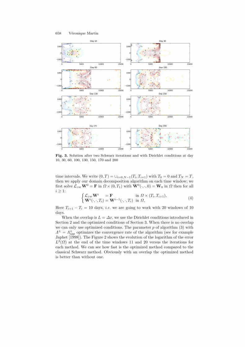
Fig. 3. Solution after two Schwarz iterations and with Dirichlet conditions at day10, 30, 60, 100, 130, 150, 170 and 200

time intervals. We write (0, T ) = ∪i=0,N−1(Ti, Ti+1) with T0 = 0 and TN = T ,then we apply our domain decomposition algorithm on each time window; wefirst solve LSW W0 = F in Ω × (0, T1) with W0(·, ·, 0) = W0 in Ω then for alli ≥ 1:

LSWWi = F in Ω × (Ti, Ti+1),Wi(·, ·, Ti) = Wi−1(·, ·, Ti) in Ω,

(4)

Here Ti+1 − Ti = 10 days, i.e. we are going to work with 20 windows of 10days.

When the overlap is L = ∆x, we use the Dirichlet conditions introduced inSection 2 and the optimized conditions of Section 3. When there is no overlapwe can only use optimized conditions. The parameter p of algorithm (3) withΛ± = Λ±

app optimizes the convergence rate of the algorithm (see for exampleJaphet [1998]). The Figure 2 shows the evolution of the logarithm of the errorL2(Ω) at the end of the time windows 11 and 20 versus the iterations foreach method. We can see how fast is the optimized method compared to theclassical Schwarz method. Obviously with an overlap the optimized methodis better than without one.

SWR Method for SW equations 659

0 5000 10000 15000

−1000

0

1000

Day 10

−4

−4

−4

−3

−3

−3

−2

−2

−2

−2

−1

−1

−1

0

0

0

22

22

3 3

3

3

4

4

4

4

5

55

6

66

7

7

8

8

99

10

11

0 5000 10000 15000

−1000

0

1000

Day 30

−4

−4

−4

−4

−4

−3

−3

−3−3

−2

−2−

1−1

0

0

22

2

22

33

3

3 3

44

4

4 4

55

55

6

6

66

77

7

8

8

9

9

10

10

11

2

2

2

3

3

3

4

4

4

5

5

6

6

7

7

8

8

9

9 101112

0 5000 10000 15000

−1000

0

1000

Day 60

−4−

3−

2−

10

2

2

2

3

2

22

2

2

22

2

3

33

3

3

333

4

4

4

4

4

4

4

4

5

5

5

5

5

6

6

6

6

7

7

7

7

8

8

8

9

9

9

10

10

10

11

11

11

12

12

13

13

14

14

15

15

16

16

0 5000 10000 15000

−1000

0

1000

Day 100

−4 −3

−2 −10

0

2 2

2 2

2

3 3

33

4 4

4 4

55

5 5

6 6

6 6

7 7

7 7

8 8

8 8

9 9

9 9

10 10

10 10

11

11

12

12

13

13

2 2

2

2

22

2

2

3

3

3

3 3 3

3

3

3

333

4

4

4

4

4 4 4

4

4

4

444

555

555

5

5

5

5

5

5

6

6

6

6

6

6

6

6

6

6

7

7

7

7

7

7

7

7

8

8

8

8

8

8

8

8

9

9

9

9

0 5000 10000 15000

−1000

0

1000

Day 130

−4

−4

−3

−3

−2

−2

−1

−1

0

0

2 2 2

2 2 2

2

2

3 3 3

3 3 3

4 4

4 4

5 5

5 5

0

0

2

2

22

2

2

2 2

22

2

22

22

2

2

33

33

33

33

3

3

3

3

3

3

3

4

4

4

4

44

4

4

5

5

5

5

5 5

5

5

6

6

6

6

6

6

7

7

7

7

7

7

8

8

0 5000 10000 15000

−1000

0

1000

Day 150

−4

−4

−3

−3

−2

−2

−1

−1

0

0

22 2

22 2

2

2

2

2

3 3

3 3

3

3

3

4

4

4

5

5

6

6

00

2

2

2

22

2 2

2

22

2

2

2

2

2

3

3

3

3

3

3

3

3 3

4

4

4

4

4

4

4

44

5

5

5

5

5

5

5

6

6

6

6

6

7

77

7

8

8

8

8

9

9

0 5000 10000 15000

−1000

0

1000

Day 170

−4

−4

−3

−3

−2

−2

−1

−1

0

0

2 2

2 2

2

2

2

2

22

33

33

44

4

4

5

5

5

5

6

6

6

6

7

7

7

7

8

8

0

0

2

22

2 2

2

2

2

22

2

2

2

2

2

2

2

2

2

2

3

3

3

3

3

3

3

33

3

3

4

4

44

4

4

4

4

5

5

55

5

5

6

6

6

6

77

0 5000 10000 15000

−1000

0

1000

Day 200

−4 −3

−3−2

−2−1

−1

0

0

2

2

2

2

2

2 2

2 2

33

33

4

4

4

4

5

5

5

5

5

6

6

6

6

77

77

00

0

0

2

2

2

2

2

2 2

2

2

2

2

2

2

2

22

3

3

3

3

3

3

3

3

33

3

3

3

3

3

3

4 4

4 4

4

4

4

4

4

4

5

5

5

5

6

6

Fig. 4. Solution after two Schwarz iterations and with optimized conditions at day10, 30, 60, 100, 130, 150, 170 and 200

For more realistic simulations where such interface conditions appear, wecan not wait for the convergence of the Schwarz algorithm because of the costof each model, and only a few iterations can be implemented. The Figures 3and 4 show the solution obtained after two Schwarz iterations in each timewindow with Dirichlet conditions or optimized one. We can see that Dirichletconditions act like a wall and waves reflect in it, whereas with optimizedconditions the solution is admittedly discontinuous at the interface but it isclosed to the monodomain solution.

5 Conclusion and perspectives

We have applied a Schwarz Waveform Relaxation method to the viscous Shal-low Water equations; we have studied the classical SWR algorithm and a anoptimized algorithm. Numerical results have shown that the optimized methodis a good one. Perspectives of that work is to improve the interface conditionsof the optimized algorithm and apply this method to the Shallow Water equa-tions linearized around any velocity field U0 6= 0.

660 Veronique Martin

References

M. J. Gander, L. Halpern, and F. Nataf. Optimal convergence for over-lapping and non-overlapping Schwarz waveform relaxation. In C.-H. Lai,P. Bjørstad, M. Cross, and O. Widlund, editors, Eleventh internationalConference of Domain Decomposition Methods. ddm.org, 1999.

M. J. Gander and A. M. Stuart. Space time continuous analysis of waveformrelaxation for the heat equation. SIAM J., 19:2014–2031, 1998.

M. J. Gander and H. Zhao. Overlapping Schwarz waveform relaxation forparabolic problems in higher dimension. In A. Handlovicova, M. Ko-mornıkova, and K. Mikula, editors, Proceedings of Algoritmy 14, pages 42–51. Slovak Technical University, September 1997.

C. Japhet. Optimized Krylov-Ventcell method. Application to convection-diffusion problems. In P. E. Bjørstad, M. S. Espedal, and D. E. Keyes,editors, Proceedings of the 9th international conference on domain decom-position methods, pages 382–389. ddm.org, 1998.

C. Japhet, F. Nataf, and F. Rogier. The optimized order 2 method. applicationto convection-diffusion problems. Future Generation Computer SystemsFUTURE, 18, 2001.

T. G. Jensen and D. A. Kopriva. Comparison of a finite difference and a spec-tral collocation reduced gravity ocean model. Modelling Marine Systems,2:25–39, 1990.

E. Lelarasmee, A. E. Ruehli, and A. L. Sangiovanni-Vincentelli. The wave-form relaxation method for time-domain analysis of large scale integratedcircuits. IEEE Trans. on CAD of IC and Syst., 1:131–145, 1982.

J.-L. Lions and E. Magenes. Nonhomogeneous Boundary Value Problems andApplications, volume I. Springer, New York, Heidelberg, Berlin, 1972.

P.-L. Lions. On the Schwarz alternating method. III: a variant for nonoverlap-ping subdomains. In T. F. Chan, R. Glowinski, J. Periaux, and O. Widlund,editors, Third International Symposium on Domain Decomposition Methodsfor Partial Differential Equations , held in Houston, Texas, March 20-22,1989, Philadelphia, PA, 1990. SIAM.

V. Martin. Methode de decomposition de domaine de type relaxation d’ondespour des equations de l’oceanographie. PhD thesis, 2003.

F. Nataf and F. Rogier. Factorization of the convection-diffusion operator andthe Schwarz algorithm. M3AS, 5(1):67–93, 1995.

J. Pedlosky. Geophysical Fluid Dynamics. Springer Verlag, New-York, 1987.A. Quarteroni and A. Valli. Domain Decomposition Methods for Partial Dif-

ferential Equations. Oxford Science Publications, 1999.H. A. Schwarz. Uber einen Grenzubergang durch alternierendes Verfahren.

Vierteljahrsschrift der Naturforschenden Gesellschaft in Zurich, 15:272–286, May 1870.

S. Vandewalle. Parallel multigrid waveform relaxation for parabolic problems.B. G. Teubner, Stuttgart, 1993.