Schwartz-Smith Two-Factor Model in the Copper Market...

School of Economics and Management

Lund University

Department of Economics

Schwartz-Smith Two-Factor Model in the

Copper Market: before and after the New

Market Dynamics

Master Thesis: NEKN02 (15 credits ECTS)

Supervisor: Karl Larsson and Rikard Green

Author: Dominice Goodwin

May 2013

Abstract.

This thesis offers a study on the performance of the short-term/long-term

model by Schwartz and Smith (2000) in the copper futures market for the period

1993-07-21 to 2013-03-05. The model's performance is evaluated in terms of its

ability to model the term structure of copper futures prices, and is for this

purpose compared to two one-factor benchmark models, an Orstein-Uhlenbeck

process and a geometric Brownian motion process. The estimated model

parameters and the generated equilibrium level and short term deviation from the

model are analyzed in order to draw conclusions about how the dynamics in the

copper market has changed over the last two decades. The results from this study

strongly support the use of a two-factor model, like the short-term/long-term

model by Schwartz and Smith (2000), for the purpose of modeling the term

structure of copper futures prices and for valuation of copper related investment

projects. The results also suggest that there has been a structural change in the

price dynamic of the copper market, which began in 2004-2005.

Key words: Schwartz-Smith Two-Factor Model, Copper, Term Structure Model.

Acknowledgments

"I would like to thank Karl Larsson and Rikard Green for being great supervisors.

I would also like to thank my girlfriend Xiaohan Li for all support."

Contents

1. Introduction ......................................................................................................................... 1

2. Theoretical background....................................................................................................... 4

2.1 An introduction to the dynamics of commodity prices .............................................. 4

2.2 Modeling the term structure of commodity futures (resent studies) .......................... 7

3. The Schwartz and Smith Two-Factor Model ...................................................................... 9

3.1 Model descriptions and specifications ......................................................................... 9

3.2 The Schwartz and Smith Two-Factor Model in State-Space form ............................ 13

4. Research Method .............................................................................................................. 15

4.1 Kalman Filter Estimation of the State Variables ....................................................... 15

4.2 Parameter Estimation ................................................................................................. 19

4.3 Performance evaluation criterions ............................................................................. 21

4.4 Data and sample period specifications ...................................................................... 23

5. Empirical Results .............................................................................................................. 25

6. Conclusions ....................................................................................................................... 35

7. Appendix ........................................................................................................................... 36

8. Bibliography ..................................................................................................................... 37

1

1. Introduction

Along with the strong economic growth in emerging markets and developing economies like

China, the close to zero interest rate environment, economic and financial crisis, and

monetary easing from central banks around the world, there has followed several noteworthy

events on the world commodity markets over the last decade. Among these are the record

breaking price increases that have occurred for many commodities. Another is the

increasingly important role commodities have earned in the alternative investments category,

so much so that commodities today are consider an asset class of its own. There has also been

an increased interest among commodity producers and consumers to managing risk on their

long term investment projects, whereby demand for longer term maturities contracts have led

to the introduction and increasing trading volumes of such contracts in several commodity

markets.

With developments of this scope in the financial and economic environment in general,

and in the commodity markets in particular, an important possible consequence to consider is

whether or not the fundamental price and volatility dynamics in the commodity markets have

changed. This is important for several reasons. One especially important reason is, however,

related to the importance stochastic modeling of commodity prices today has in derivatives

pricing, investment valuation and heading decisions. Since the outputs from pricing and

valuation models that incorporates some stochastic model in a fundamental way depend on

the chosen stochastic processes, there lies a clear economic value in assessing a stochastic

model that in a parsimonious yet accurate way describes the true dynamics of the underlying

commodity. A valid hypothesis to investigate is therefore whether or not the price and

volatility dynamics in the commodity markets have change, and if so is the case, how these

dynamics has changes. Or maybe more concretely, to investigate whether or not the today

popular models for modeling commodity prices, which were developed before these

potentially new dynamics, still are appropriate for their intended purposes.

For some commodities, crude oil being one example, such studies, and development of

new models, appear more frequently than for others. Among the commodities that have been

given the least attention in this regard, when taken their traded volumes in spot and futures

markets into consideration, are non-ferrous metals. The aim of this thesis is therefore to

conduct such a study for copper, which is the most traded non-ferrous metal on the London

metal exchange.

2

To do so, one of the most popular models for modeling commodity prices, namely the

short-term/long-term model by Schwartz and Smith (2000), commonly referred to as the

Schwartz-Smith two-factor model, will be evaluated in the copper market before and after

these new market dynamics are thought to have begun.

The aim of the study in this thesis is, in other words, therefore to investigate, firstly,

whether or not the Schwartz-Smith two-factor model is an appropriate model for modeling

copper prices, and how the model's performance in doing so has changed over time. And

secondly, in the light of the estimation results from the Schwartz-Smith two-factor model,

investigate how the dynamics in the copper market have changes over time in terms of mean-

reversion, risk-premium, convenience yeild and changes in the copper equilibrium price.

The value of such a study lies, to begin with, in the argumentation related to the potentially

new market dynamics above. It should however also be noted that there seems to be a total

lack of published studies where the performance of the Schwartz-Smith two-factor model in

modeling non-ferrous metals is investigated. For this reason, evaluating the Schwartz-Smith

two-factor model in the copper market is probably the main contribution to the literature by

the study in this thesis.

The reason for selecting the Schwartz-Smith two-factor model for the study, except for

being one of the most popular models for modeling commodity price, is because that the

model in its original form was developed for modeling crude oil prices, whereby the model

should have a fairly good potential to model copper prices, since both crude oil and copper are

storable commodities without seasonal price patterns. Furthermore, due to the construction

and properties of the Schwartz-Smith two-factor model, the model displays results in a way

that is intuitional and highly informative for the purpose of analyzing market dynamics.

Finally, in September 2002 a 63 months to maturity futures contract was introduced for

copper at the London metal exchange (LME). Since there at this date exist a sufficiently large

time period of daily price observations for this contract, the possibility now exists to analyze

how well the Schwartz-Smith two-factor model are able to model also these long term futures

contracts in the copper market.

To investigate the research objective of this thesis the model parameters and the two factors of

the Schwartz-Smith two-factor model was estimated in three different datasets. The first

dataset included data of daily closing price observations for spot and futures contracts that

where traded at LME between 1993-07-21 and 2002-09-27. In this dataset price data for four

contracts were available: 3 Months U$/MT, 15 Months U$/MT and 27 Months U$/MT and

3

Cash U$/MT. The second dataset included price observations for the same contracts between

2002-09-30 and 2013-03-05. The third dataset were identical to the second dataset with the

only difference being that the 63 Months U$/MT contract was included here.

For each of these datasets the economical and statistical significance of the model

parameters were analyzed. The estimated equilibrium price and the deviations from this

equilibrium price were also analyzed for signs of new dynamics in the copper market. Finally,

the models ability to model the term structure of copper futures prices was investigated by

comparing the model to the two one-factor models − an Orstein-Uhlenbeck process and a

geometric Brownian motion process − out of which the Schwartz-Smith two-factor model is

constructed. This is motivated by the fact that the result from such a model comparison yields

the answer to whether or not the Schwartz-Smith two-factor model delivers any significant

improvements to either of these two one-factor models.

The remainder of this thesis is divided into five sections. Section 2 gives a brief introduction

to the topic of modeling the term structure of commodity futures prices. This section does also

provide an incomplete list of some recent and important works in this field. Section 3 covers

the model descriptions and specifications of the Schwartz-Smith two-factor model, which is

intended to serve as a foundation for the description of the research methodology in section 4

and the interpretation of the empirical results in section 5. Section 6 summarizes the

conclusions that could be made from the analysis of the empirical results.

4

2. Theoretical background

2.1 An introduction to the dynamics of commodity prices

Researchers have recognized that commodities are different from other classes of assets in

several fundamental aspects and that these differences should be considered when

selecting/developing a stochastic model for commodity prices. Commodities are, to begin

with, physically produced, making their prices dependent on the cost of production, and

current and expected future scarcity. Most commodities are also consumption goods, meaning

that they are primarily bought and held with the purposed of being consumed, for example as

an input in a production chain. The production level, cost of production and the consumption

demand can furthermore vary significantly in seasonal patterns. There are also significant

costs and risks associated with storing (holding inventories of) commodities, for example

warehouse costs and risk of deterioration. For some commodities, such as electricity, these

storage costs are so high that these commodities have to be produced and consumed close to

simultaneously.

These are some of the special properties that commodities have, and it's not hard to

imagine why these properties would have an impact on the market price and volatility

dynamics, and why commodities might experience different price dynamics than those of

investment assets. In fact, for storable consumption commodities like copper, which is the

focus of this thesis, there has for long been observed that the dynamics are not of the kind that

is commonly assumed for investment assets.

To begin with, when observing the term structure (that is, the relationship between the spot

price and the futures prices for different maturities at a given date) of these commodities over

time it can been seen that the term structure from time to time have a downward sloping

shape, commonly referred to as 'backwardation', which violates the simple cost-of-carry

arbitrage relationship for investment assets. For futures contracts with some financial

investment asset (e.g. equities, bonds, etc.) as underlying, the arbitrage free price can be

derived from the current spot price, interest rate and yield obtained from holding the asset.

Formally,

, where is the value of a futures contract today that matures in T periods; is the current

spot price; is the periodic continuously compounded interest rate; is the periodic

5

continuously compounded yield rate. This arbitrage relationship is upheld by the argument

that, for assets which are held solely with the purpose of generating a return (the definition of

investment assets) investors are indifferent between holding the asset or the future contract as

long as the return generated is the same (J. C. Hull (2008), p.99-118). Under this arbitrage-

free relationship the term structure is straight upward sloping line when working in

logarithmic prices.

Explanations for the negatively sloped term structure for commodities originates in the

famous concepts of: the "supply of storage" theory by Williams (1936), "convenience yield"

by Kaldor (1939), the "price of storage" theory by Working (1948 and 1949), the theory of

"normal backwardation" by Keynes (1930), and others.

From these theories there have emerged two distinctive classes of models that are used for

modeling the term structure of commodity futures prices.1 One of these, convenience yield

models, which originates in the theories of Kaldor (1939) and Working (1948), links the

futures prices to the current spot price by taking into account the net cost/benefit of holding

the physical asset compared to holding the future contract. This net cost/benefit includes

interest rate, storage costs, and a convenience yield. Formally,

, where is the value of a futures contract today that matures in T periods; is the current

spot price; is the periodic continuously compounded interest rate; is the proportional

periodic continuously compounded cost of storage; and is the periodic continuously

compounded convenience yield. Here and are written as constants, but are modeled as

time and/or maturity dependent or stochastically, as will be discussed shortly.

In this context backwardation is explained by a convenience yield that exceeds the sum of

the interest rate and storage costs. The existence of a convenience yield is commonly

explained by the argument that both commodity producers and consumers should find a value

in having an inventory of the commodity to meet unexpected demand and to lower stock-out-

risk. This value, or equivalently the convenience yield, has been suggested to depend on

markets expectations of current and future availability/scarcity of the commodity and current

1 See for example J. C. Hull (2008) p.115-121 for a more detailed discussion about these two classes.

6

inventory levels (low levels of inventories and/or expectations of scarcity implies high

convenience yield).2

In the second class, risk premium models, which originates from Keynes (1930) and Hicks

(1939), future prices are given by the discounted (by a risk premium) expected future spot

price. Formally,

, where is the value of a futures contract today that matures in T periods, is the

conditional expectation of the spot price at time T, and is the periodic continuously

compounded risk premium. As will be described in more detail in section 3 of this thesis,

Schwartz-Smith two-factor model employs this risk premium relationship to value futures

contracts and to model the term structure.

Another important dynamic for commodity prices is that the term structure changes over time,

from contango to backwardation, and vise versa. One way to view this is that the short-term

prices are mean reverting, where the mean is given by some equilibrium price. Or,

alternatively, that the size of the convenience yield evolves over time.

This mean reverting property of commodity prices is commonly explained through the

argument that divergences form a long term equilibrium price can occur due to some supply

or demand shock which is of a temporary nature. Such temporary change in the supply or

demand could for example be coursed by unusual weather or political instabilities. When this

supply or demand shock is temporary, the scarcity or abundance of the commodity it

generates should be temporary as well, therefore only causing the near term prices to be

affected.

In a situation where such a temporary chock causes price to increase to a level above the

long term equilibrium price, supply is then expected to increase since higher cost producers,

which could not operate profitable in the market before, now will enter the market. Old

production technologies which were expected to go offline can now also stay in operation

longer. This would then consequently put downward pressure on the price until it reaches the

same or a new equilibrium level. By the same logic an upward pressure on the price is

expected to occur when the price is below some equilibrium price level. When this 'correction'

2 The "theory of storage" developed by Working (1949), Brennan (1958), and Telser (1958) suggesting a

negatively sloped and convex term structure in situations of low inventories and near term scarcity.

7

in the price is not instantaneous, and assuming that the equilibrium price is fairly stable, one

could expect to observe mean reversion in the short term prices.

The equilibrium price, which the short term prices revert towards, is thought to be

determined by the cost of production under normal circumstances, and the markets

expectation of the future supply and demand of the commodity in the long term.

2.2 Modeling the term structure of commodity futures (resent studies)

Over the last two to three decades there has been a large number of models developed which

has aimed to model commodity prices according to these know dynamics. Below follows a

short literature review of some of the more recently published important works in this area.3

Gibson and Schwartz (1990) acknowledged that the convenience yield was evolving

stochastically and developed a two factor model for oil prices. They modeled the spot price as

a geometric Brownian motion, and the convenience yield using a mean reverting stochastic

process.

Schwartz (1997) developed a three factor model where the spot price, convenience yield

and interest rate were modeled stochastically. He analyzed the model using weekly data of

futures prices for crude oil, copper and gold (between 1985 and 1995), and concluded that a

model consisting of all three factors did not produce significantly better fit to the observed

futures price and volatility term structure than did a model consisting of only the first two-

factors. This two factor model did however perform significantly better than did a model

consisting of only the first factor, the spot price, modeled as a mean reverting stochastic

process. He therefore concluded that interest rate was not an important factor to include in

term structure models for commodities. Also, a two factor model was to prefer to a one-factor

model.

The short-term/long-term model by Schwartz and Smith (2000), commonly referred to as

the Schwartz-Smith two-factor model, is one of the most popular models for modeling

commodity prices.4 Although Schwartz and Smith (2000) originally developed and used the

model for modeling crude oil prices, a number of extensions to the model have been

developed and the model is today used for modeling prices of several important commodities.

3 Lautier (2003) provides a more extensive review on the main contributions to the literature on term structure

models for commodity prices.

4 This model is the working model of this thesis and will be covered more details in section 3 of this thesis.

8

Following the publication of the Schwartz-Smith two-factor model several researcher have

used this model. Manoliu and Tompaidis (2002) used it to analyze natural gas prices.

Sorensen (2002) analyzed agricultural commodities. Lucia and Schwartz (2001) and

Villaplana (2004) analyzed electricity markets. Aiube, Baidya and Tito (2008) extended the

model with a jump factor.

Schwartz and Trolle (2009) developed a model for pricing commodity derivatives in which

the volatility is modeled stochastically.

M. Haase and H. Zimmermann (2011) developed a two-factor model where the spot price

is decomposed into a pure asset component and a scarcity related component, and where the

risk premium of commodity futures is directly related to a scarcity related component.

Aiube (2012) analyzed the empirical performance of an extended version of the Schwartz-

Smith two-factor model in which the drift rate of the long-term component was modeled

stochastically as a third factor. He analyzed this models fit to the long-term crude oil future

contracts (60 and 67 months) by comparing it to the original Schwartz-Smith two-factor

model. He found that the two-factor model underestimated the risk premium and had worse fit

to long term contracts (both prices and volatilities) compared to the three factor model.

9

3. The Schwartz and Smith Two-Factor Model

This section provides a description of the short-term/long-term model by Schwartz and Smith

(2000). This description includes a summary of the structure and properties of the model,

which is intended to serve as a foundation for the description of the research methodology (in

section 4) and the interpretation of the empirical results (in section 5).

3.1 Model descriptions and specifications

The short-term/long-term model (referred to as the S&S-model in the remainder of this thesis)

by Schwartz and Smith (2000) is a two factor model for modeling commodity spot prices.

With this model Schwartz and Smith introduced a new way of thinking about the stochastic

behavior of commodity prices, namely that the spot prices can be decomposed into short-term

and a long-term component to be modeled with stochastic processes according to their

individual dynamics.

More specifically, the spot price of a commodity at time , denoted , is decomposed into

two factors, a long-term equilibrium price ( ) and a short-term deviation from this

equilibrium price ( ). The long-term equilibrium price ( ) is assumed to follow a geometric

Brownian motion process, and the short-term deviation ( ) is assumed to revert towards zero,

following an Ornstein-Uhlenbeck process. The sum of these two factors gives the logarithm

of the spot price. Formally,

.

(3.1.1)

.

(3.1.2)

(3.1.3)

, where and are increments of a standard Brownian motion process, which are

assumed to be correlated ( ). is a mean-reversion coefficient, the size of

which determines the rate at which reverts towards zero.5 , and are restricted to

positive values.

5 To clarify why the short term deviation revert towards zero, consider the more general definition of the

Ornstein-Uhlenbeck process: . We arrive at the expression in eq. 3.1.3 by setting

the long-term mean ( ), which the process revert towards, equal to zero.

10

Through the process for short-term deviation ( ) the model allows for changes in the spot

price which are not expected to persist in the long run, and specifies the way in which these

short run deviations from the equilibrium price are expected to disappear. And, through the

process for equilibrium price level ( ), which separates the S&S-model from the class of pure

mean-reversion models, the it also allows for the possibility that changes in the spot price are

of a long-term nature. By this construction, the model allow for mean-reversion in short-term

prices and uncertainty in, and evolution of, the equilibrium price, a model structure that are in

line with the inherent uncertainty of equilibrium prices and the at the time (year 2000)

apparent mean-reversion in prices for most commodities.

As is apparent from eq. 3.1.1-3 the S&S-model does not explicitly model the convenience

yeild. Schwartz and Smith (2000) do however show that the model is equivalent to the

stochastic convenience yield model of Gibson and Schwartz (1990), but with the difference

being that changes in short-term futures prices are interpreted short-term price variations

rather than changes in the instantaneous convenience yeild.

Schwartz and Smith (2000) provided a few augments to why this new structure would be

useful. To begin with, thinking in terms of a stochastically evolving short term deviation and

equilibrium price might be more intuitional than to be thinking in terms of a stochastically

evolving convenience yeild and spot price. Secondly, Schwartz and Smith (2000) showed that

the short term deviation and equilibrium price were more orthogonal in there dynamics than

were the convenience yeild and spot price in the Gibson and Schwartz (1990) model, a model

property that leads to more transparent analytical results and makes it easier to analyze the

individual impact of the two factors. Furthermore, since the short-term deviation is expected

to disappear, only the long term factor determents the long term expected prices and the

volatility in these long term price, thereby making the model more suitable for valuing long-

term commodity related investments.

Based on the defined processes in equation 3.1.2 and 3.1.3 Schwartz and Smith (2000)

derived the expressions for the expected future spot price and the variance of this prediction.

First, from equation 3.1.2 and 3.1.3, and were shown to be jointly normally distributed,

with

,

(3.1.4)

11

(3.1.5)

, where and are the today's (initial) values of the two factors.

And, from equations 3.1.1, 3.1.4 and 3.1.5, the log of the spot price is then normally

distributed, and the spot price log-normally distributed, with

,

(3.1.6)

(3.1.7)

To use this commodity spot price model to value future contracts, options one these futures

contracts and other commodity related derivatives and investment projects, Schwartz and

Smith (2000) developed a 'risk-neutral' version of the model as shown by equation 3.1.8 and

3.1.9 below.

,

.

(3.1.8)

(3.1.9)

Here the two additional parameters, and , represents risk premiums.6

and are

again increments of a standard Brownian motion process with

.

In this risk-neutral version of the model the short-term deviations ( ) revert towards

, and the equilibrium price level ( ) has a drift rate of . And, under these

risk-neutral processes, Schwartz and Smith (2000) showed that and are jointly normally

distributed with

,

(3.1.10)

(3.1.11)

6 These risk premiums constitutes constant reductions in the drift rates of the two stochastic processes in the

model of the 'true' spot price. Schwartz and Smith (2000) motivates this method of risk adjustment by assuming

that the two state variables are priced according to the intertemporal asset pricing models developed in Merton

(1973) and Cox et al. (1850). Although only this basic model will be used in this thesis, Schwartz and Smith

(2000) did propose a way to let vary with the short term deviations.

12

Therefore, the log of the future spot price under risk-neutrality is normally distributed with

,

.

(3.1.12)

(3.1.13)

Since, under the risk-neutral framework, future prices are equal to the risk neutral expected

spot price, the relationship between the futures prices and the spot price can be derived from

equation 3.1.12-13 as

(3.1.14)

, where

Structuring equation 3.1.14 in the way above using is convenient when expressing the

model in state-space form, as will be shown in section 3.2 below.

From equation 3.1.14 it can be seen that depend on , the model parameters, and the

equilibrium price level ( ) and the short-term deviation ( ). Thus, for a given set of model

parameters and values of the two factors, a term structure for the futures prices can be

generated for a specific set of different values of . This allows one to value futures contract

for any given , including for which there are no futures contracts trading, which is useful

for real asset and investment valuation. The benefit of being able to model the entire term

structure is hereby evident.

To value futures contracts and model the term structure with the S&S-model in this way it

is, however, required that the model's parameters and the current value of the two factors are

known. Generally the model's parameters are not known and have to be estimated. The

equilibrium price level and the short-term deviation are, furthermore, not directly observable

and must therefore also be estimated in some way. For this purpose the S&S-model uses the

Kalman filter, a procedure that will be described in section 4.1 and 4.2.

Using the relationship between the spot price and the futures prices in equation 3.1.14 the

Kalman filter estimation of the S&S-model's parameters and the two factors are based on

historically observed prices of futures contracts for different maturities (and spot prices if

such are available). The underlying idea behind this is that information about these factors

13

should be incorporated in the observed term structure. More specifically, changes in the price

of long-maturity futures contract can be interpreted as price changes which the market expects

to persist in the long term (changes in the equilibrium price). And, changes in the difference

between long-term and short term futures prices can be interpreted as price changes which the

market expects to be of a temporary nature (changes in the short-term deviations).

3.2 The Schwartz and Smith Two-Factor Model in State-Space form

Before describing how the Kalman filter can be used for estimating the parameters and the

two unobservable factors of the S&S-model, it is convenient to first see how the S&S-model

can be written in state-space form. By, treating the S&S-model's two factors, ( ) and ( ), as

state variables, we get that the transition equation and the measurement equation for the S&S-

model can be written as eq. 4.1 and eq. 4.2 below.

, (3.2.1)

, (3.2.2)

, where

, a 2 1 vector of state

variables;

, 2 1 vector;

, a 2 2 matrix;

is a 2 1 vector of disturbances;

length of each time steps;

number of time periods in the data

set.

, a n 1 vector

of observed log future prices with

maturities

, n 1 vector;

, n 2 matrix;

is a n 1 vector of disturbances;

number of future contracts

In the transition equation the state transition matrix and vector specifies how the 'true' and

unobservable state vector ( ) is expected to evolve from one time step to another. This

transition dynamic of the state vector is directly given by the derived mean vector for the two

factors in the S&S-model (eq. 3.1.4). The disturbances in vector are assumed to be

normally distributed and serially uncorrelated, with and

as given by eq. 3.1.5. The transition equation is therefore simply equation

3.1.4 and equation 3.1.5 rewritten as a first order stochastic difference equation.

14

In the measurement equation the transformation matrix and vector maps the state

vector into the measurement domain. This allows the estimated system states at time to be

transformed into a prediction for the measurement observations at time , which in turn can be

compared with the actual measurement observations ( ). The residuals from this

measurement prediction (measurement errors), the terms in vector , are assumed to be

normally distributed and serially uncorrelated, with and . In this thesis

it is for simplicity further assumed, just as it was in Schwartz and Smith (2000), that is

diagonal. Finally, and are assumed to be independent of each other and uncorrelated

with the initial state at all time periods.

It can also be worth pointing out that this model can be estimated using a simple linear and

time-invariant version of the Kalman filter. By working and in logarithmic prices the

transition and measurement equation becomes linear, which is a requirement for the basic

form of Kalman filter estimation of the state vector. This form of the S&S-model does also

assume constant covariance, as can be seen from the lack of a time subscript on and .

15

4. Research Method

In the empirical study of this thesis the S&S-model's unknown parameters and unobservable

factors, ( ) and ( ) were estimated in three different datasets of futures contracts prices. The

unknown parameters were estimated through the use of the Kalman filter and maximum

likelihood estimation. Estimates of the two unobservable factors were then, through Kalman

filtering, generated based on these estimated model parameters. This section provides an

overview of this methodology. For details and more extensive coverage of the Kalman

Filtering technique, see for example A.C. Harvey (1989) and J.D. Hamilton (1994).

This section also provides specifications of what data that was used in each of the three

estimations, and descriptions of the statistical test that was employed to evaluate the

estimation results.

It should also be mentioned that all estimations were done in Matlab, using a code that was

written over the course of writing this thesis. It has been written as a function in a general way

with detailed instructions so that anyone who wishes estimate the S&S-model can do so using

this function. The code along with a manual and the data used in this thesis can also be found

at Matlab's file exchange under the name 'ss2000estim.m'.

4.1 Kalman Filter Estimation of the State Variables

The Kalman filter, by R. E. Kalman (1960), is a data processing algorithm for recursively

computing an optimal estimator for the states of a linear dynamical system expressed in state-

space form. To be more concrete, the Kalman filter computes an updated (posterior)

prediction of a state vector's mean and covariance at time , conditional on all information

available up to and including time . This information includes; [1] a (priori) prediction for

the state vector's mean and covariance at time , computed form the state vector's mean and

covariance at time 1 and the specified stochastic processes for the state variables in the

transition equation; [2] measurement observations at time , for which a linear relationship to

the state variables (and the uncertainty in this relationship) can be specified. The Kalman filter

algorithm combines, in accordance with Bayes's theorem, these two pieces of information

about the state vector's mean and covariance time in order to minimize the uncertainty

(covariance) in the updated (posterior) estimator. Priori and posteriori do in this context refer

to the two situations; before and after the measurement at time has been observed.

16

A central assumption of the Kalman filter is that the initial distribution of the state vector,

and all state variables and measurement variables are normally (or multivariate normally)

distributed. This assumption is necessary to derive the Kalman filter, and gives it several

desirable properties which are worth pointing out, even though the properties of the Kalman

filter is not the main focus of this thesis.

To begin with, under this assumption the priori and posteriori predictions of the state

vector's mean and covariance gives conditional distributions for the state vector (since normal

distributions are fully described by its mean and variance). This is useful since it opens up for

further inference about the state vector than just providing point estimates.

Secondly, under the normality assumption the mean of this posteriori conditional

distribution is the best linear unbiased estimator (BLUE) of the state vector at time ,

conditional on all information available up to and including . Although the estimator is not

unbiased when the normality assumption is dropped, this estimator still has minimum mean

square errors among all linear estimators. The Kalman filter is thus optimal in the sense that it

minimizes the mean square errors in the class of linear estimators.

And finally, under this assumption the measurement errors can be shown to be normally

distributed, whereby a likelihood function can be constructed conditional on a dataset of

measurements, a set of parameter values and a measurement covariance matrix. In this way

the Kalman filter also provides the possibility to estimate the unknown parameters of the

system. This process will be described further in section 4.2.

Now, moving on to describe the process of using the Kalman filter to recursively estimate the

two unobservable factors in the S&S-model. Before observing for a given , our estimator

of the state vector's distribution at time has to be computed based on the transition equation

alone. The priori estimator for the state vector's distribution is, in other words, computed from

the transition dynamics of the state vector as specified by transition equation (eq. 3.2.1). The

priori estimator for the state vector's mean is given by taking the expectation of equation

3.2.1, and using that , which gives:

(4.1.1)

, where denotes the information set available at time 1, and is the posteriori

estimator for the state vector's mean from the previous period, formally;

. The recursive property of the Kalman filter is here self explanatory. The

17

criterion used in this thesis for selecting an initial distribution of the state vector is specified in

section 4.3.

The priori estimator for the state vector's covariance matrix is also derived from the

transition equation (eq. 3.2.1), and can be written as: 7

(4.1.2)

, where is the covariance matrix for the posteriori distribution in the previous period.

To generate the updated, or a posteriori, estimator for the state vector's distribution, the

priori distribution, from eq. 4.1.1 and 4.1.2 above, first is transformed into the same units as

that of the measurements.8 The convention here is to map the state vector's distribution into

the measurement domain, which is the purpose of the measurement equation (eq. 3.2.1).

Using the measurement equation, the estimator for the vector of measurements ( )

and the corresponding covariance matrix ( ) at time , can be shown to be:

(4.1.3)

(4.1.4)

7 Note that the prediction error can be simplified to: . The cross product

terms disappear since it is assumed that the estimation errors and the process noise term, , are uncorrelated:

.

8 In the literature describing the Kalman filter there are several commonly mentioned ways to think about why

this is necessary. One is to think about it in the terms of that the Kalman filter computes the posteriori

distribution using a prediction-error correction type estimation, where 'error' is refer to the observed

measurement at time minus the predicted value of the measurement at time This predicted measurement is

then given by mapping the priori estimator for the state vector into the measurement domain. The Kalman filter

then computes the posteriori estimator as a weighted average of the priori distribution and the prediction of the

state vector which is suggested by the observed measurement, where the weight given to the priori estimator is

inversely proportional to the size of prediction error. A second way of thinking about this is simply that, for two

normal distributions to multiply together, they need to be in the same units. Since the measurements are assumed

to be normally distributed and the elements in measurement error covariance matrix ( ) are expected to be none

zero, the measurements at time created a normal conditional distribution for the state vector at time , but in the

measurement domain.

18

, , and are assumed to be symmetrical since they are all covariance

matrices.

The Kalman filter now computes the posteriori distribution for the state vector. The

derivation of the Kalman Filter algorithm can be done in a number of different ways.

Following the example shown by Hamilton (1994) chapter 14, the posteriori distribution can

be computed through the formula for updating a linear projection as

(4.1.5)

The variance-covariance matrix of this updated estimator for the state vector, defined as ,

is:

(4.1.6)

By defining , equation 4.1.5 and 4.1.6 above can be rewritten in the

following way, as was used by Schwartz and Smith (2000),

;

.

(4.1.7)

(4.1.8)

The posteriori distribution, as given by the Kalman filter (equation 4.1.5 and 4.1.6) is then

used as an input in equation 4.1.1 and 4.1.2 to compute the priori distribution for the next time

step. As is apparent now, the Kalman filter computes the posteriori distribution for each ,

19

where is given by the number of measurement vector observations ( ). And,

at each the posteriori distribution incorporates all information about the state vector that

have been available up to and including time , without increasing the complexity of the

computation or the result since one at each is left with a normal distribution. One does in

other words not need all the previous data to compute the next priori and posteriori

distribution, which give the Kalman Filter its recursive property, which in the engineering

literature is referred to as online estimation, meaning that the Kalman filer can update the

prediction about the state variables as soon as a new measurement vector is observed.

4.2 Parameter Estimation

The Kalman filter estimation of the unobservable factors, ( ) and ( ), the process which has

just been described in the previous section, requires that all model parameters (

) and the terms in the measurement covariance matrix ( ) are known. Or, in other

words, the Kalman filter recursively computes estimates for and in form of a posteriori

conditional distribution, and does so based on a given dataset of spot and/or futures prices, a

set of model parameters, and a given measurement covariance matrix ( ).

In the case when the model parameters and the measurement covariance matrix are not

known, they can be estimated through maximum likelihood estimation. Denoting the diagonal

elements in measurement covariance matrix ( ) by

, a log-likelihood function is

maximized with respect to

. Assuming

that the measurement errors are normally distributed and using the log-likelihood function

suggested by A. C. Harvey (1988 p.126) for this maximum likelihood estimation, this

problem can formally be expressed

(4.2.1)

, where is the determinant of , and are the errors between the observed spot

and future prices and the predicted prices as given by equation 4.1.3. This log-likelihood

function can be maximized numerically by rerunning the Kalman filter for different values of

20

.9 In this thesis this log-likelihood function was maximized using the interior-point algorithm

with the fmincon function in Matlab.

To maximize this log-likelihood function some restrictions has to be set on some of the

parameters. The restrictions used for the parameter estimation in this thesis are specified in

table 4.2.1 below.

Table 4.2.1 - Parameter boundaries for maximum likelihood estimation

Boundaries κ S1-Sn

Upper Inf Inf Inf Inf Inf Inf 1 Inf

Lower 0 0 -Inf -Inf 0 -Inf -1 0 Note: Inf (infinite) means that the parameters are not being restricted.

As was mentioned in the previous section, an initial distribution for the state vector, given by

its mean and covariance at = 0, has to be know (or assumed) in order to run the Kalman

filter. Judging by the literature it does not seems that there exist a clear consensus regarding

how one is to best select this initial value.10

However, since the covariance matrix for the

posteriori distribution ( ) approaches a asymptotical value after running the Kalman filter

for a while, this value appeared to be a good guess, and was therefore used as the initial

covariance matrix ( ) in this thesis. Furthermore, since the short term deviation is assumed

to be mean reverting, the best guess for its initial value should probably be zero. In this thesis

the initial value for the posteriori mean vector was therefore set to: .

The estimation does also require an initial . Here it should be important to point out that

several local maximum was found depending on the initial value of . A large number of

initial was therefore tested in order to find a global maximum. It should also be important to

mentioned that the final parameter estimates ( ) was quite sensitive to the initial .

The standard errors for were obtained from the hessian. However, since the model

estimates the parameters so that the one or a couple of futures contracts are matched with

close to zero measurement errors, the measurement error covariance matrix V is positive

9 This iterative process, where the Kalman filter and maximum likelihood estimation are combined, is sometimes

referred to as the expectation maximization algorithm or prediction error decomposition.

10 It does however exist some suggestions on how one could achieve a good guess for this initial distribution.

One such example is the two stage estimation procedure proposed by T. Perez, G. C. Goodwin, and B. Godoy

(2009).

21

semi-defined in all of the estimations.11

This was also found by Schwartz and Smith (2000) in

their estimation of the model on oil futures contracts. To be able to invert the hessian and

obtain standard errors for a rather ad hoc solution was employed in this thesis. Once it

was known which of the future contracts that were matched with close to zero measurement

errors, the estimation was redone with the corresponding elements in measurement error

covariance matrix V restricted to zero and excluded from . In this way V was positive

defined and invertible. However, the parameter estimated ( ) presented in the results in

section 5 are from the original estimation where all parameters where included in the

estimation, and only the standard errors were taken from this ad hoc solution estimation.

Finally it can also be mentioned that the Matlab code written for estimations in this thesis

was tested on the crude oil data used in Schwartz and Smith (2000) as to make sure it was

error free. Both parameter values and standard errors were very similar to those that Schwartz

and Smith (2000) found.

4.3 Performance evaluation criterions

To evaluate the performance of the S&S-model in the Copper market the statistical and

economic significance of the estimated parameters will, to begin with, be investigated. Then,

to conclude whether or not the S&S-model performs better than a simple one-factor model,

the two one-factor models which the S&S-model consists of, the geometric Brownian motion

and the Ornstein-Uhlenbeck, will be estimated and used as benchmarks.

Since the S&S-model consists of these two one factor models they can be estimated by

restricting on some of the parameters in the S&S-model, in addition to the restrictions on the

other parameters as given by table 4.2.1. The geometric Brownian motion is estimated by

restricting , , and all elements except second diagonal element of to zero. The

Ornstein-Uhlenbeck model is estimated by restricting , , and all elements except first

diagonal element of to zero. Under these restrictions the Ornstein-Uhlenbeck model will

have a constant equilibrium level, which has to be estimated in advance. In this thesis this

constant equilibrium level is simply set to the average equilibrium level of the S&S-model,

11

As Schwartz and Smith (2000) pointed out, up to two contracts can always be perfectly matched by the model

by specifying measurement error covariance matrix V so that the measurement error variance for these two

contracts are restricted to zero.

22

whereby the Ornstein-Uhlenbeck model probably will reach its maximum potential as a

benchmark.

The two one-factor models are restricted versions of the S&S-model, therefore a

significantly higher likelihood score can be interpreted as that the additional parameters

provides statistically significant improvements to the models fit to the observed spot and

futures prices. This statistical significance is tested using likelihood ratio test, where the

likelihood ratio statistic is compared to a chi-squared distribution with two degrees of freedom

when comparing the S&S-model to the geometric Brownian motion model and three degrees

of freedom when comparing the S&S-model to the Ornstein-Uhlenbeck model.

Although comparing the likelihood scores will provide useful information, it is important

to consider what these likelihood scores actually measures. As can be seen in log-likelihood

function (equation 4.2.1) the errors ( are the errors between the predicted futures prices

from the priori distribution and the observed futures prices. The likelihood score is thus a

measure of how well the priori prediction of the futures prices has been in the data sample. It

might, however, also be interesting to see how well each model is able to model the observed

term structure given the best prediction of the models factor(s), that is, how well the posteriori

prediction of the futures and spot prices matches the observed. These errors do not contain the

errors in the forecasting which is case with the errors from the priori distribution. Instead, the

errors between the posteriori prediction of the futures and spot prices and the observed prices

show only how well the models are able to model the term structure of the futures prices

given the best current prediction of the factor(s). It should thus be informative to compare the

models' performance in terms of both the likelihood scores and the term structure fit given the

posteriori prediction of the model factor(s).

To obtain the posteriori prediction of the futures and spot prices the posteriori prediction

of the state variables can be mapped into the measurement domain in the same way as the

priori prediction of the state variables was in equation 4.1.3. This can be written formally as,

(4.3.1)

The errors between these predicted spot and future prices and the observed spot and future

prices are analyzed in terms of mean absolute error, standard deviation of error and mean

error. These statistics are presented under 'term structure fit' in section 5.

23

4.4 Data and sample period specifications

As was mentioned above and in section 3, the S&S-model uses observations of spot and/or

futures contracts prices as inputs to estimate the model's unknown parameters and the two

unobservable factors at each time step. The data used for the study in this thesis consists of

daily closing prices for futures contracts on copper (U$/MT), which were traded at London

Metal Exchange between 1993-07-21 and 2013-03-05 (Source of data: Datastream).

In order to investigate how the model's performance has changed over time, the sample

was divided into two subsamples. The first sample ranges from 1993-07-21 to 2002-09-27

(2320 observations), and the second sample from 2002-09-30 to 2013-03-05 (2635

observations). Separating the sample at this point is motivated by the fact that the 63 months

future contract for copper where introduced 2002-09-30, thereby allowing for the use of this

contract in the estimation of the model in the second sample. In total the model will therefore

be estimated on three different data sets.

In the first dataset there is available price data for futures contracts of three different

maturities, 3 Months U$/MT, 15 Months U$/MT and 27 Months U$/MT, plus the Cash

U$/MT. In the second dataset there is available price data for the same futures contracts as in

the first sample, plus the 63 Months U$/MT. Table 4.4.1 below summarizes what data will be

used in each data set.

Table 4.4.1 - Specification of datasets for the three estimation periods

Dataset 1 Dataset 2 Dataset 3

Time period: 1993-07-21 - 2002-09-30 - 2002-09-30 -

2002-09-27 2013-03-05 2013-03-05

Future Contracts: Cash Cash Cash

3 Months 3 Months 3 Months



63 Months

Note: The Cash contract is in this thesis treated as a spot price.

In the remainder of this thesis these futures contracts may be referred to as Cash, 3M … 63M,

and in the estimation they correspond to the terms in the measurement error covariance

parameters (

) so that Cash corresponds to and the future contract with the

longest maturity corresponds to .

24

It should also be noted that, in the LME data obtained from Datastream, it appeared to be

daily closing prices for days when LME had not been open. Around specific dates, Christmas,

New Year and Easter holidays and so on, the prices had not been updated. Since it make no

sense to keep these days in the data for the estimations they were deleted from the data. The

rule that was used to determine whether or not a day was to be counted as a closed day, was if

neither of the price of the Cash, 3M, 15M or 27M contract had been updated that day. In total

165 days where deleted and a list of all deleted days can be found in Appendix table 4.4.2.

25

5. Empirical Results

Tables 5.1-3 on the following three pages display the estimated model parameters and

corresponding standard errors for the maximum likelihood estimations in the three datasets. In

the upper part of figures 5.1-3 the equilibrium price, estimated spot price (given by ),

and observed spot price (Cash) are plotted over the sample periods. The lower part of these

figures shows the difference between Cash and the price of the future contract with the

longest (Cash minus 27M or 63M) in order to demonstrate the current situation in terms of

"contango vs. backwardation". Tables 5.4-7, on the page following these figures, display the

results from the model comparisons.

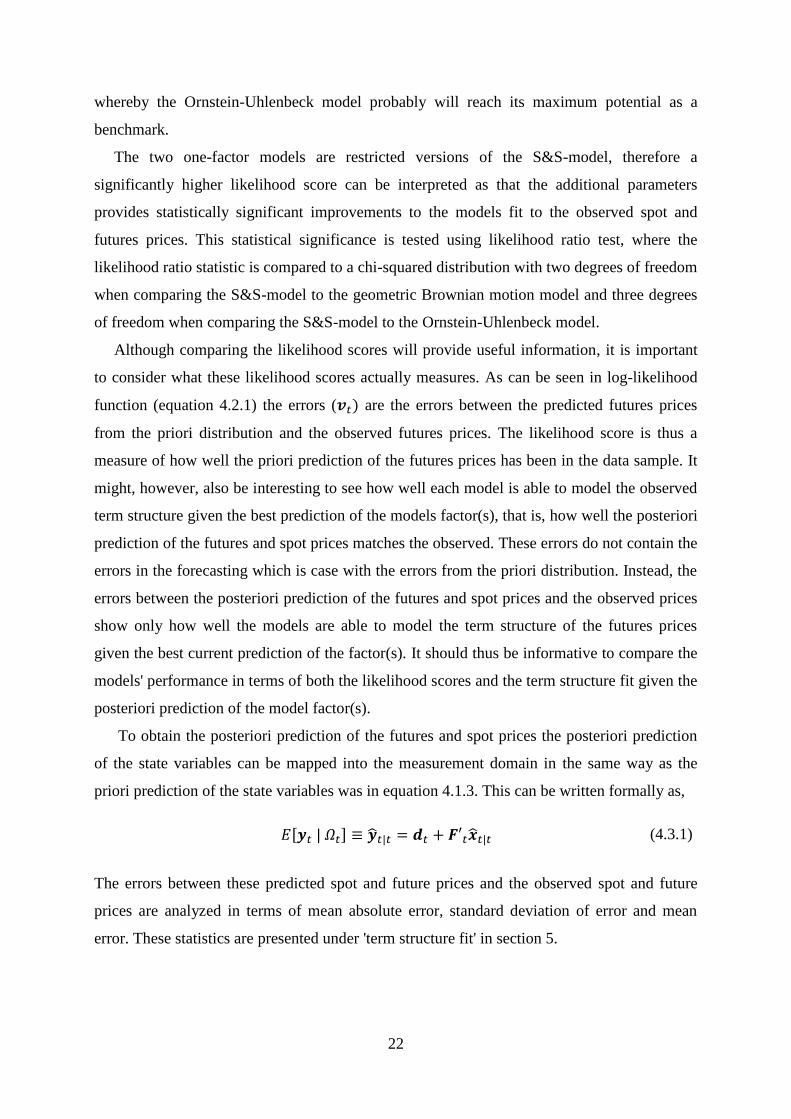
By visually analyzing figures 5.1-3 it can in see that prices in first period (dataset 1) were

fluctuated around a long term price of about 1700 U$/MT. During the sharp price increases

that began in 1994 due to an improving world economy, the term structure transitioned from

maximum contango to heavy backwardation. Doing so, the long term prices increased less

than did the short term, thereby helping the model to distinguish between changes in the

equilibrium price and the short term deviation. The market and the model predicted that much

of the price increases were of a temporary nature. During this period there were reports of that

inventory levels where decreasing and the observed backwardation is thus in line with the

theory of storage. An alternative way of viewing these substantial short term deviations is

therefore that the market perceived a short term scarcity which along with decreasing

inventory levels had the effect of sharply increasing the convenience yield in the copper

market.

In the second half of the first period short term deviations were much smaller. The model

appears to predict a zero short term deviation when the term structure is close to maximum

contango. In these situations, and when the short term prices are decreasing, the equilibrium

price therefore seems to move together with the short term prices, with a limited size of the

negative short term deviation.

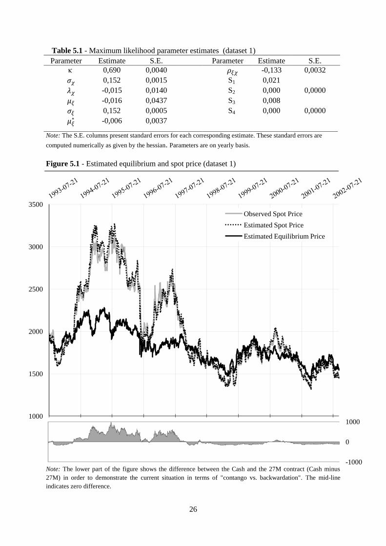
In the second period (dataset 2) it is apparent that there has occurred some kind of

structural shift in the copper market around year 2004-2005. Around year 2004 prices were at

the 3000 U$/MT level, as they were under the 1994-1995 period. And just as during the 1994-

1995 period the market seem to have predicted that much of the price increases were of a

temporary nature, and the term structure transitioned from maximum contango to heavy

backwardation.

26

1000

1500

2000

2500

3000

3500

Observed Spot Price

Estimated Spot Price

Estimated Equilibrium Price

-1000

0

1000

Table 5.1 - Maximum likelihood parameter estimates (dataset 1)

Parameter Estimate S.E. Parameter Estimate S.E.

κ 0,690 0,0040 -0,133 0,0032

0,152 0,0015 S1 0,021

-0,015 0,0140 S2 0,000 0,0000

-0,016 0,0437 S3 0,008

0,152 0,0005 S4 0,000 0,0000

-0,006 0,0037

Note: The S.E. columns present standard errors for each corresponding estimate. These standard errors are

computed numerically as given by the hessian. Parameters are on yearly basis.

Figure 5.1 - Estimated equilibrium and spot price (dataset 1)

Note: The lower part of the figure shows the difference between the Cash and the 27M contract (Cash minus

27M) in order to demonstrate the current situation in terms of "contango vs. backwardation". The mid-line

indicates zero difference.

27

1000

3000

5000

7000

9000

11000

Observed Spot Price



-500

2500


Parameter Estimate S.E.


κ 0.338 0,0026 -0.209 0,0027

0.204 0,0035 S1 0.000 0,0000

-0.101 0,0048 S2 0.007

0.183 0,1115 S3 0.000 0,0000

0.288 0,0015 S4 0.027

-0.085 0,0062







28

1000

3000

5000

7000

9000

11000

Observed Spot Price



-1000

5000




κ 0,212 0,0045 -0,458 0,0098

0,283 0,0056 S1 0,011 0,0000

-0,075 0,0037 S2 0,000

0,263 0,0745 S3 0,014 0,0000

0,310 0,0048 S4 0,000

-0,065 0,0015 S5 0,073 0,0001







29

Table 5.4 - log-likelihood scores

Model Dataset1 Dataset2 Dataset3

S&S Two-factor model 29829 32626 35547

Brownian motion 16050 15311 18697

Ornstein-Uhlenbeck 22729 19170 19552

Table 5.5 - Term structure fit (dataset 1)

Contract

maturity

Mean Absolute Error

Std. of Error

Mean Error

S&S GBM OU S&S GBM OU S&S GBM OU

Cash

0,014 0,096 0,014

0,020 0,115 0,020

-0,006 0,005 -0,003

3M

0,000 0,080 0,000

0,000 0,096 0,000

0,000 0,006 0,000

15M

0,006 0,028 0,019

0,008 0,032 0,025

-0,001 -0,002 -0,004

27M 0,000 0,001 0,027 0,000 0,001 0,033 0,000 0,000 0,003 Note: S&S: S&S Two-factor model, GBM: geometric Brownian motion, OU: Ornstein-Uhlenbeck.


Contract

maturity

Mean Absolute Error

Std. of Error

Mean Error


Cash

0,000 0,102 0,015

0,000 0,116 0,018

0,000 -0,001 -0,002

3M

0,005 0,089 0,000

0,007 0,101 0,000

0,002 0,002 0,000

15M

0,000 0,036 0,053

0,000 0,042 0,063

0,000 0,000 -0,003

27M 0,020 0,006 0,093 0,026 0,008 0,106 0,003 0,000 -0,005 Note: S&S: S&S Two-factor model, GBM: geometric Brownian motion, OU: Ornstein-Uhlenbeck.


Contract

maturity

Mean Absolute Error

Std. of Error

Mean Error


Cash

0,008 0,104 0,015

0,011 0,120 0,018

-0,003 0,003 -0,002

3M

0,000 0,091 0,000

0,000 0,105 0,000

0,000 0,005 0,000

15M

0,010 0,039 0,053

0,014 0,045 0,063

-0,001 0,002 -0,004

27M

0,000 0,002 0,093

0,000 0,003 0,106

0,000 0,000 -0,006

63M 0,058 0,094 0,182 0,074 0,117 0,209 0,005 0,011 0,004 Note: S&S: S&S Two-factor model, GBM: geometric Brownian motion, OU: Ornstein-Uhlenbeck.

30

This time however, the prices kept rising, and in late 2005 the market's perception of that the

price increases were of a temporary nature seems to have shifted to a belief that it instead was

the long term price of copper that was increasing. Between October 2005 and the following

six months the long term prices were increasing more than the already rapidly increasing short

term prices, causing the estimated equilibrium price to pike up from about 1700 U$/MT to

near 5000 U$/MT. Following this 'catch up' by the long term prices, the short term prices now

spiked up to record breaking levels near the 9000 U$/MT mark in the summer of 2006,

leading to a unprecedented level of backwardation. Due to the construction of the S&S-model

this development can in a clear way be interpreted as that the market during this period both

perceived the long term equilibrium price in the copper market to be increasing, and that there

was a severe near term shortage. An interesting question to ask here is whether any of this

development, especially the spike in the short term prices after the 'catch up' by the long term

prices, was driven by speculations. This question is, however, out of the scope of this thesis to

answer.

Over the subsequent two and a half years, leading up to the financial crisis of 2008, the

spot price where significantly higher than the equilibrium price. The spot price dipped back

down towards the equilibrium price two times before, at the third time, crash down right

through the suggested equilibrium level during the outbreak of the financial crisis in

September 2008. This event highlights the fact discussed before, that in situations where the

short term prices are decreasing, the equilibrium move together with the short term prices due

to the limited possible magnitude of contango in the term structure. It can however be noted

that the term structure exhibited a record breaking size of contango during the crash, which

possibly could be explained by market participant's fear (speculations) of further price

decreases had a dominant effect compared to the will and ability of exercising carry trades.

In the soon four years that has followed the crash of 2008, there seem to have developed

another kind of dynamics in the copper market. The short and the long term prices are moving

together also when the short term prices increases rapidly, whereby the equilibrium price

follows the spot price more closely. This could be interpreted as that the market expects the

recent year's extraordinary price increase in the copper market to stay for a foreseeable future.

This argument can be further motivated by looking at the figure for dataset 3, where the

estimated equilibrium level was much more conservative in the price increase during 2005-

2008 compared to the price increase that has followed the crash of 2008. Even when the 63M

contract is included, the estimated equilibrium level was at the end of the second period (Mars

2013) close to 7000 U$/MT.

31

Finally it should be pointed out that the 'spiky' black boarder in the lower part of the figure

for the last three years in this dataset 3 is a consequence of a diminishing trading volume in

the 63M contract. Although this might lead to unreliable parameter estimates, estimating the

model in dataset 3 brings at least support for the argument discussed above.

Moving on to investigate the economic and statistical significance of the estimated model

parameters, we see that, κ, , , and the terms in the measurement covariance

matrix are estimated with high precision in all three datasets. , on the other hand, is

estimated with low precision. This was also the case in Schwartz and Smith (2000) and Aiube

(2012). This fact is explained by that the process for which is the growth rate, the price

expectation (eq. 3.1.6), never is observed and thus can't be estimated with high precision.

However, as Schwartz and Smith (2000) pointed out, the low accuracy of the estimate of

do not have any negative consequences for valuation purposes.

is not estimated with much precision in dataset 1. This is in line with the argumentation

in Schwartz and Smith (2000), that can't be estimated with much precision since both

and describes the difference between the expected prices and the future prices, and since

price expectations are not observed, these risk premiums can't be estimated with much

precision. However, is estimated with precision in dataset 2-3. A significant was also

found by Aiube (2012). This contradicts the argument by Schwartz and Smith (2000), and

might be explained by that in fact can be estimated through the observed future prices

since it constitutes a part of the intercept of the long term futures price ( ( ), eq. 3.13).

The accuracy in the estimate of might thus depend on the accuracy in the estimates of ,

and .

Looking at the sizes of the volatility parameters for the equilibrium price and the short

term deviation, and , we see that these are much larger in sample 2-3 than in sample 1.

The mean reversion parameter (κ) is furthermore about two times as large in sample 1

compared to sample 2. These results are in line what one might expect by analyzing the

figures visually. Dataset 1 is characterized by more mean reversion and lower volatility than

dataset 2-3.

In dataset 1 is estimated to negative 1.6 %, due to the slightly decreasing equilibrium

level ( ) over the period. Here is estimated to negative 0.6%, which translates into an

estimated of negative 1 %. Schwartz and Smith (2000) did also find a negative due to

32

the negative and pointed out that this is not likely to be representative of investors

expected growth rate over the period. A close to zero in dataset 1 can probably be

explained by that the term structure in this dataset was equally much in contango and

backwardation.

In dataset 2-3 on the other hand, which is an extraordinary period in terms of increased

price and backwardation, the equilibrium price have increased dramatically. In dataset 2-3

is estimated to about 20 %. And, as a consequence of the magnitude and consistency in the

backwardation, the term structure should for most part have a negative slope, thereby causing

to be negative. As expected,

is estimated to about negative 7 %, translating into a of

about 30 %. It should however be noted that, since can't be estimated with much accuracy,

the estimates of are unreliable as well.

It is hard to draw any conclusions regarding the risk premium in dataset 1 due to the

statistical insignificance of and in. Although is estimated with much higher accuracy

in dataset 2-3, it is hard to derive a meaningful economic interpretation of its size and sign in

separation of . The reason for this is that, although this short term risk premium is negative

the aggregated risk premium might not be so. The aggregated risk premium can be derived

from equation 3.1.12, and written as

(5.1.1)

, and in fact, given the estimated model parameters in dataset 2-3, this aggregated risk

premium is positive for any positive value of .

It is hard to think of any economic reason for the negative correlation parameter ( ) in

all three samples. This might instead be a symptom of that the model to some degree fails to

filter out whether or not the change in the spot price was due to a change in the equilibrium

price or the short term deviation. A motivation for this argument is that the correlation

parameter tends to be estimated to minus 1 when the model is estimated on short periods of

data where there is little difference in the movements in the long and short term prices.

Finally, investigating the log-likelihood scores and the statistics for the term structure fit in

tables 5.4-7, it is clear that the S&S-model dominates the two one-factor models. In table 5.4

we see that the S&S-model has significantly higher log-likelihood scores in each of the three

datasets. The difference between the S&S-model and the two one-factor models is,

33

furthermore, larger in dataset 2-3 than in dataset 1. An interesting observation here is that the

Ornstein-Uhlenbeck (OU) model performed significantly better compared to the geometric

Brownian motion model (GBM) in all three datasets. The difference between these two

models are however less in dataset 3 than in the first two datasets.

These findings can be explained by considering the shape of the term structure that each

model suggests, and the data on which these models have been estimated. The shape of the

term structure given by the GBM model is simply a straight line with a time-0 intercept at the

logarithm of the current spot price. Thus, the poor performance of the geometric Brownian

motion model should not come as a surprise when considering the frequency and magnitude

of the transitions between backwardation and contango that is present in each dataset. Fitting

a straight line with a constant slope through a time series of the term structure under such

conditions are bound to produce errors, especially in the short term futures prices. A lower

likelihood score in dataset 2 than in dataset 1, despite more observations in dataset 2, can

therefore be explained by the even stronger presence of these dynamics. However, the

increased likelihood score in dataset 3 can probably be explained by that a larger portion of

the observations are given by long term contracts (since the 63M contract is included in this

dataset), and that the straight line term structure given by the GBM more accurately models

these long term prices.

The term structure suggested by the OU model, on the other hand, allows for mean

reversion in the prices around a straight line with a zero slope and a constant time-0 intercept,

which corresponds to the constant equilibrium level. The OU model does in other words allow

for the changes between contango and backwardation over time. With this in mind it is not

surprising that the OU model performs much better in dataset 1 compared to in dataset 2,

since the OU model does not allow for a changing equilibrium price over time. Due to this

property of the OU model, the model fails to accurately model long term prices if these are

non-stationary, which can explain the lower performance in dataset 2-3.

The analysis made above, on the basis of the likelihood scores, is supported by the results

for the term structure fit for the three models in table 4.5-7. As is evident from the mean

absolute errors and standard deviation of errors in these tables, the GBM model is able to fit

the short term prices poorly and the long term prices much better. This is the case in all of the

three datasets. The opposite is true for the OU model. By looking at the mean errors it is also

clear that the OU model consequently have a downward bias in its predicted term structure for

dataset 2-3. This expected since the model wasn't able to adjust the equilibrium level in a

period of strong price increases. However, the most important result here is that the S&S-

34

model is able to fit both the short and the long term contracts well. In fact, in most cases the

S&S-model is able to fit the short term prices better than the OU and the long term prices

better than the GBM.

35

6. Conclusions

It is clear that there has been some kind of structural change of the price dynamics in the

copper market. The equilibrium price, which was rather stable around 1700 U$/MT between

1993 and 2004, increase rapidly (by about 18.5 % annually) up to about 6000 U$/MT between

2005 and 2013.The most noteworthy change in the dynamics in this new environment is that

the short and the long term prices are moving synchronized together, whereby the equilibrium

price follows the spot price more tightly, a fact that probably can be interpreted as that market

participants now seem to believe that the recent years (2009-2013) price increases are of a

permanent nature. These change can probably be summarized as a transition away from mean

reverting dynamic (in the short-term) around a rather stable long term equilibrium price,

towards a dynamic where both the short term prices and the long term equilibrium price have

a significant upwards trend.

It can also be concluded that the Schwartz-Smith two-factor model are to be strongly

recommended for modeling the term structure of futures prices in the copper market,

compared to using either of the two one-factor benchmark models (the Ornstein-Uhlenbeck

model and the geometric Brownian motion model). The Schwartz-Smith two-factor model

dominated these two one-factor model in terms of both likelihood scores in the maximum

likelihood estimation of the model parameters, and in terms of its ability to model the term

structure. In fact, the Schwartz-Smith two-factor model was able to model the term structure

better across all maturities compared to the two one-factor models.

All parameters that are important for valuation purposes in the Schwartz-Smith two-factor

model could, furthermore, be estimated with precision. It was, however, not possible to draw

any strong conclusions regarding the risk premium or convenience yeild due to the statistical

insignificance of the estimated risk premium parameters.

36

7. Appendix

Table 4.4.2 - List of deleted dates from Datastream data

1993-08-30 1997-12-25 2001-08-27 2005-03-28 2009-04-13

1993-12-27 1997-12-26 2001-12-24 2005-05-02 2009-05-04

1993-12-28 1998-01-01 2001-12-25 2005-05-30 2009-05-25

1994-01-03 1998-01-02 2001-12-26 2005-08-29 2009-08-31

1994-04-01 1998-04-10 2001-12-31 2005-12-26 2009-12-25

1994-04-04 1998-04-13 2002-01-01 2005-12-27 2009-12-28

1994-05-02 1998-05-04 2002-03-29 2006-01-02 2010-01-01

1994-05-30 1998-05-25 2002-04-01 2006-04-14 2010-04-02

1994-08-29 1998-08-31 2002-05-06 2006-04-17 2010-04-05

1994-12-26 1998-12-25 2002-06-03 2006-05-01 2010-05-03

1994-12-27 1998-12-28 2002-06-04 2006-05-29 2010-05-31

1995-01-02 1999-01-01 2002-08-26 2006-08-28 2010-08-30

1995-04-14 1999-04-02 2002-12-25 2006-12-25 2010-12-27

1995-04-17 1999-04-05 2002-12-26 2006-12-26 2010-12-28

1995-05-08 1999-05-03 2002-12-27 2007-01-01 2011-01-03

1995-05-29 1999-05-31 2003-01-01 2007-04-06 2011-04-22

1995-08-28 1999-08-30 2003-04-18 2007-04-09 2011-04-25

1995-12-25 1999-12-27 2003-04-21 2007-05-07 2011-04-29

1995-12-26 1999-12-28 2003-05-05 2007-05-28 2011-05-02

1996-01-01 1999-12-31 2003-05-26 2007-08-27 2011-05-30

1996-04-05 2000-01-03 2003-08-25 2007-12-24 2011-08-29

1996-04-08 2000-04-21 2003-12-25 2007-12-25 2011-12-26

1996-05-06 2000-04-24 2003-12-26 2007-12-26 2011-12-27

1996-05-27 2000-05-01 2004-01-01 2008-01-01 2012-01-02

1996-08-26 2000-05-29 2004-04-09 2008-03-21 2012-04-06

1996-12-25 2000-08-28 2004-04-12 2008-03-24 2012-04-09

1996-12-26 2000-12-25 2004-05-03 2008-05-05 2012-05-07

1997-01-01 2000-12-26 2004-05-31 2008-05-26 2012-06-04

1997-03-28 2001-01-01 2004-08-30 2008-08-25 2012-06-05

1997-03-31 2001-04-13 2004-12-27 2008-12-25 2012-08-27

1997-05-05 2001-04-16 2004-12-28 2008-12-26 2012-12-25

1997-05-26 2001-05-07 2005-01-03 2009-01-01 2012-12-26

1997-08-25 2001-05-28 2005-03-25 2009-04-10 2013-01-01

37

8. Bibliography

Printed sources:

M. J. Brennan (1958), "The Supply of Storage", The American Economic Review, 48(1), 50-

72.

F.A.L. Aiube, T.K.N. Daidya, and E.A.H. Tito (2008), "Analysis of commodity prices with

the particle filter ", Energy Economics, 30 (2008) 597-605.

R. Gibson and E.S. Schwartz (1990), "Stochastic convenience yield and the pricing of oil

contingent claims", Journal of Finance, 45: 959-76.

J.D. Hamilton (1994), "Time Series Analysis", Princeton University Press.

A.C. Harvey (1989), "Forecasting, structural time series models and the Kalman filter",

Cambridge University Press.

J. Hicks (1939), "Value and Capital".

J.C. Hull (2008), "Options, Futures, and other Derivatives", Pearson Prentice Hall, 7th

edition.

R.E. Kalman (1960), "A New Approach to Linear Filtering and Prediction Problems," Journal

of Basic Engineering, 82, 34-45.

J.M. Keynes (1930), "A Treatise on Money: The applied Theory of Money", Londres,

Macmillan, vol. 2.

N. Kaldor (1939), “Speculation and Economic Stability”, Review of Economics Studies, 7:1-

27.

J. J. Lucia and E. S. Schwartz (2001), "Electricity prices and power derivatives: evidence

from the Nordic Power Exchange", Review of Derivatives Research, 5(1), 5-50.

M. Manoliu and S. Tompaidis (2000), "Energy futures prices: Term structure models with

Kaman filter estimation", University of Texas, Austin.

T. Perez, G. C. Goodwin, and B. Godoy, (2009), "Parameter Estimation of Structural

Commodity Price Models", International Federation of Automatic Control (IFAC),

Proceedings of the 15th IFAC Symposium on System Identification (Saint-Malo, France 6-8

July, 2009), p. 1429-1434.

E.S. Schwartz (1997), "The stochastic behavior of commodity prices: implications for

valuation and hedging", Journal of Finance, 52, 923-973.

38

E.S. Schwartz & J.E. Smith (2000), "Short-term variations and long-term dynamics in

commodity prices", Management Science, 46, 893-911.

C. Sorensen (2002), "Modeling seasonality in agricultural commodity futures", Journal of

Futures Markets, 22, 393-426.

J.B. Williams (1936), “Speculation and the Carryover”, Quarterly Journal of Economics, 50:

436-455.

H. Working (1948), “Theory of the inverse carrying charge in futures markets.” Journal of

Farm Economics, 30: 1–28.

H. Working (1949), “The theory of price of storage”, American Economic Review, 39: 1254–

1262.

L. G. Telser (1958), "Futures Trading and the Storage of Cotton and Wheat", The Journal of

Political Economy, 66(3), 233-255.

A. Trolle and E. Schwartz (2009), "Unspanned Stochastic Volatility and the Pricing of

Commodity Derivatives", Review of Financial Studies, Vol. 22 p4423-446.

P. Villaplana (2004), "Pricing power derivatives: a two-factor jump-diffusion approach", Eighth

Real Options Conference, Montreal, Canada.

Online sources:

F.A.L. Aiube (2012), "On the comparison of Schwartz and Smith's two and three-factor

models on commodity prices",

http://www.google.se/url?sa=t&rct=j&q=&esrc=s&source=web&cd=2&cad=rja&ved=0C

DgQFjAB&url=http%3A%2F%2Fbibliotecadigital.fgv.br%2Focs%2Findex.php%2Fsbe%2F

EBE12%2Fpaper%2Fdownload%2F3753%2F1457&ei=h8mjUczpAqX44QSr-

YAg&usg=AFQjCNEVmA8LBHI5_b3XeqA5l8n9OXOWYQ&sig2=NcFgYhUSoO8GqgUFc3o

Dig&bvm=bv.47008514,d.bGE

D. Lautier (2003), "Term structure models of commodity price",

http://basepub.dauphine.fr/bitstream/handle/123456789/5465/Term%20structure%20models.

pdf?sequence=1.

M. Haase and H. Zimmermann (2011), "Scarcity, Risk Premiums and the Pricing of

Commodity Futures: The Case of Crude Oil Contracts",

http://www.unifr.ch/controlling/seminar/20102011/Haase%20Zimmermann%20ScarCommPa

per.pdf

Schwartz-Smith Two-Factor Model in the Copper Market...

Documents

Transcript of Schwartz-Smith Two-Factor Model in the Copper Market...