SCHRODINGER EQUATIONS FOR HYDROGEN

MOLECULAR IONS

by

Louis Michel Ritchie

June 22, 2020

Report presented for the degree of ICFP Master 2 in PhysicsIntership Supervisor: Jean-Philippe Karr

Laboratoire Kastler Brossel, Sorbonne University

Contents

1 Introduction 2

2 Variational solution of the three-body Schrodinger equation 3

3 Results 6

3.1 Non Born-Oppenheimer curves . . . . . . . . . . . . . . . . . . . . 6

3.1.1 Convergence . . . . . . . . . . . . . . . . . . . . . . . . . . . 6

3.1.2 Vibrational Wavefunctions . . . . . . . . . . . . . . . . . . . 7

3.1.3 Comparison to the Adiabatic curve . . . . . . . . . . . . . . 7

3.2 Analytical Electronic Potential . . . . . . . . . . . . . . . . . . . . . 8

4 Conclusion 14

I Appendix . . . . . . . . . . . . . . . . . . . . . . . . . . . . . . . . 16

1

Chapter 1

Introduction

The Born-Oppenheimer (BO) approximation is a widely used approximation inmolecular physics [1]. It assumes that the nuclear and electronic motions can beseparated, due to the nuclear mass being much larger than the electronic mass.This allows the Schrodinger equation for the electron to be solved in the staticfield of two fixed nuclei. This approximation greatly simplifies calculations butthe accuracy is limited to ∼

(mM

), or roughly 10−3 (where m is the electron mass

and M is the reduced nuclear mass,) since we ignore the nuclear kinetic energieswhen solving the Schrodinger equation. The precision can be improved by in-cluding corrections to the BO picture (also called “non-adiabatic corrections”) ina perturbative expansion in powers of m

M. However, this becomes quite tedious

when going to high perturbative orders. Alternatively,one can use a non-BO ap-proach [2] where the coupled motion of every particle in the molecule is included.This can give extremely accurate solutions but is more computationally difficult.

The Hydrogen molecular ion (HMI), H+2 is the simplest molecule found in na-

ture, composed of two protons and a single electron. It often serves as a benchmarksystem in quantum chemistry and has been studied theoretically since the begin-nings of quantum mechanics in the late 1920’s [3]. In this study, we calculate thepotential energy curves (PEC) of H+

2 from a full three-body approach i.e. thatincludes effects beyond the BO approximation in an attempt to improve on thecommonly used Born-Oppenheimer approximation and compare them to a BOcurve that includes ‘adiabatic’ corrections, i.e. that includes the averaged nuclearkinetic energy. As an exploratory idea we also attempt to obtain a non-adiabaticcorrection potential for the electron from the non-BO potential curves.

2

Chapter 2

Variational solution of thethree-body Schrodinger equation

The Schrodinger equation for a three-body diatomic system with nuclear chargesZ1 and Z2 and one electron with charge Z3, such as H+

2 is,(− 1

2m13

∇2R −

1

2m23

∇2r1− 1

m3

∇R∇r1 +Z1Z3

R+Z2Z3

r1+Z1Z2

r2

)Ψ = EΨ (2.1)

where for the hydrogen molecular ion m13 = memp

me+mpis the proton-electron reduced

mass and the distances r1, r2 and R are defined in Figure 2.1.Most of the high precision calculations performed on three-body systems such asH+

2 have been based on a variational approach [4]. The variational principle statesthat for a normalisable wavefunction Ψ, the quantity,

E =〈Ψ|H|Ψ〉〈Ψ|Ψ〉

(2.2)

provides an upper bound to the true ground state E0, i.e. E ≥ E0.In theapproach used here, the wavefunction (for angular momentum L = 0 so weonly have the radial component) can be expanded in a basis set of exponentialfunctions,

Ψ(r1, r2, R) =N∑n=1

{CnRe

(e−αnr1−βnr2−γnR

)+DnIm

(e−αnr1−βnr2−γnR

)}(2.3)

The exponents αn, βn, γn are complex numbers, however in practice only γn mustbe complex to reproduce the oscillating behaviour of the vibrational wavefunction.These exponents are pseudo-randomly generated in several intervals, the bounds

3

4

of which act as variational parameters to be optimised. Finding the extrema ofE in (2.2) with respect to the linear parameters Cn, Dn, i.e. solving the set ofequations ∂E

∂Cn= 0 is equivalent to solving a generalised eigenvalue problem,

Hc = λOc (2.4)

where c is a vector of coefficients (Ψ =∑N

i=1 ciΨi), H is the Hamiltonian ma-trix with elements Hij = 〈Ψi|H|Ψj〉 and O is the overlap matrix Oij = 〈Ψi|ψj〉.The lowest of the eigenvalues λ0 is an upper bound to E0. In addition to thisthe remaining eigenvalues λ1, λ2 . . . are also upper bounds to the exact energiesE1, E2 . . . [4].

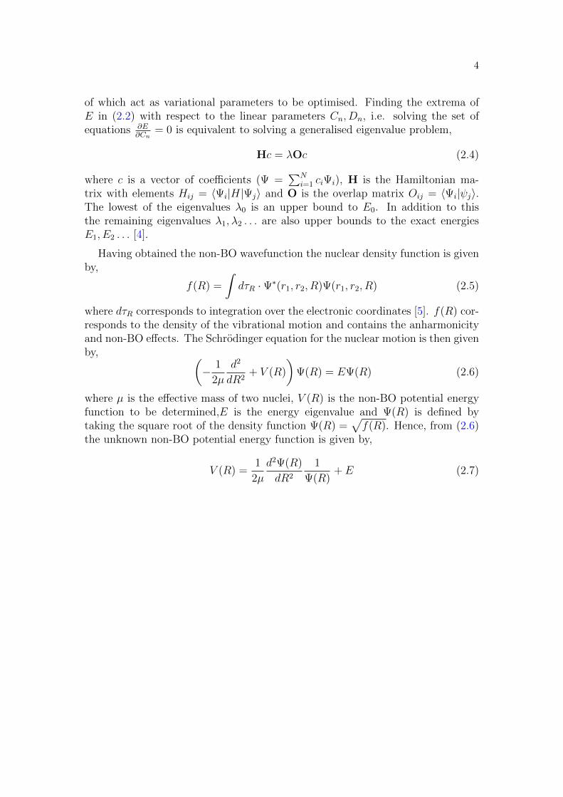
Having obtained the non-BO wavefunction the nuclear density function is givenby,

f(R) =

∫dτR ·Ψ∗(r1, r2, R)Ψ(r1, r2, R) (2.5)

where dτR corresponds to integration over the electronic coordinates [5]. f(R) cor-responds to the density of the vibrational motion and contains the anharmonicityand non-BO effects. The Schrodinger equation for the nuclear motion is then givenby, (

− 1

2µ

d2

dR2+ V (R)

)Ψ(R) = EΨ(R) (2.6)

where µ is the effective mass of two nuclei, V (R) is the non-BO potential energyfunction to be determined,E is the energy eigenvalue and Ψ(R) is defined bytaking the square root of the density function Ψ(R) =

√f(R). Hence, from (2.6)

the unknown non-BO potential energy function is given by,

V (R) =1

2µ

d2Ψ(R)

dR2

1

Ψ(R)+ E (2.7)

5

Figure 2.1: The three body diagram for a diatomic molecule with one electron. Ris the internuclear distance, and r1, r2 are the the distances from nucleus 1 and 2to the electron respectively.

Chapter 3

Results

3.1 Non Born-Oppenheimer curves

In this section we describe the non-BO results obtained using the variationalmethod with exponential basis sets explained above in §2. We first discuss theconvergence of the potentials, then the vibrational wavefunctions, and finally wecompare our results to the BO approximation with adiabatic corrections.

3.1.1 Convergence

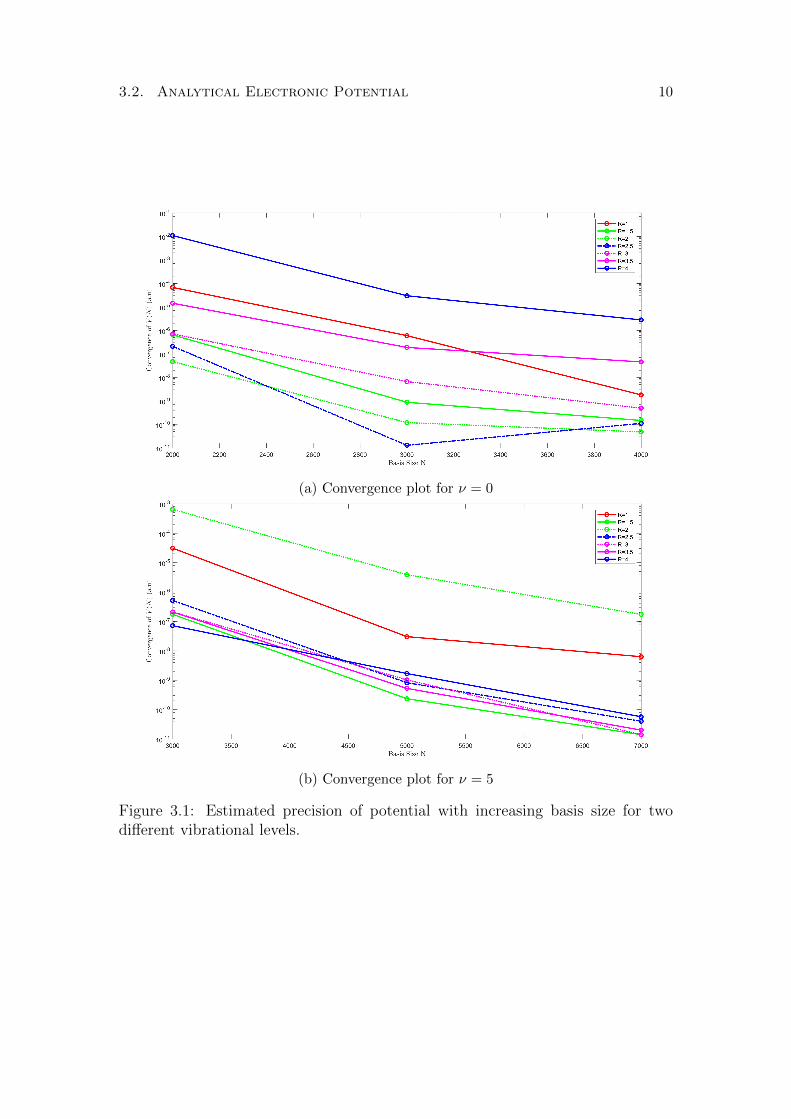
In the non-BO calculations we choose a basis size N . Table 3.1 shows the energylevel as a function of increasing basis size for two different vibrational levels. Fig-ure 3.1 shows the successive differences in the non-BO potential as the basis sizeis increased for several values of the internuclear distance R and for two differentvalues of ν. As the basis size increased the difference in the calculated potentialdecreased for a given R, that is the potentials converged. From these figures wecan estimate the precision to be on the order of a few 10−11. For some values ofR the convergence is significantly worse, for example in Figure 3.1a, for R = 4the precision is quite low. This is because the vibrational wavefunction for ν = 0is very close 0 at R = 4 (shown in Figure 3.2), hence the potential is imprecise.Likewise for R = 2 for ν = 5 in Figure 3.1b. We also see that convergence becomesmuch slower as the vibrational level is increased (See Table 3.1), hence for higherν-states we chose a maximum basis size of N = 6000.

6

3.1. Non Born-Oppenheimer curves 7

Table 3.1: Convergence of the Energy level with increasing Basis size N , for twodifferent vibrational states. The convergence of the energy level is slower for largerν states.

Vibrational state ν Basis size N Energy (a.u)

ν = 01000 -0.59713906295554382000 -0.59713906308137523000 -0.59713906308137674000 -0.5971390630813767

ν = 51000 -0.55284074170544173000 -0.55284074991111755000 -0.55284074991111847000 -0.5528407499111184

3.1.2 Vibrational Wavefunctions

Figure 3.2 shows the non-BO wavefunctions at vibrational levels ν = 0 to 11 forthe ground electronic state. In general for a state ν the wavefunctions have νnodes and ν + 1 peaks. The vibrational motion is anharmonic, so as ν increasesthe centre of the vibrational wavefunctions shifts to the right and the furthestpeak on the right (large R) becomes larger, so as the vibrational level increases itbecomes more likely for the nuclei to be further apart.

3.1.3 Comparison to the Adiabatic curve

Figure 3.3 shows the difference between the non-BO curves we have calculated forthe different vibrational levels and the potential energy curve calculated with adi-abatic corrections, i.e. that includes the average nuclear kinetic energy. Note thatby solving the Schrodinger equation in one of these potentials e.g. ν = 0,we willobtain the exact vibrational wavefuntion for the ν = 0 state,but not for the otherν states. As the vibrational level increases more and more holes start appearingin the potential curves. This is because as ν increases the number of nodes (placeswhere the wavefunction goes to zero) in the vibrational wavefunction increases,and since the potential (recall (2.7)) is undefined when Ψ → 0 we experience nu-merical precision problems, so the points in the vicinity of nodes are discarded.We also see that the differences between the non-BO curves and the adiabaticcurve are on the order on 10−6a.u which reflects the fact that the adiabatic curveis accurate to ∼

(mM

)2, whereas the non-BO curves are exact.

3.2. Analytical Electronic Potential 8

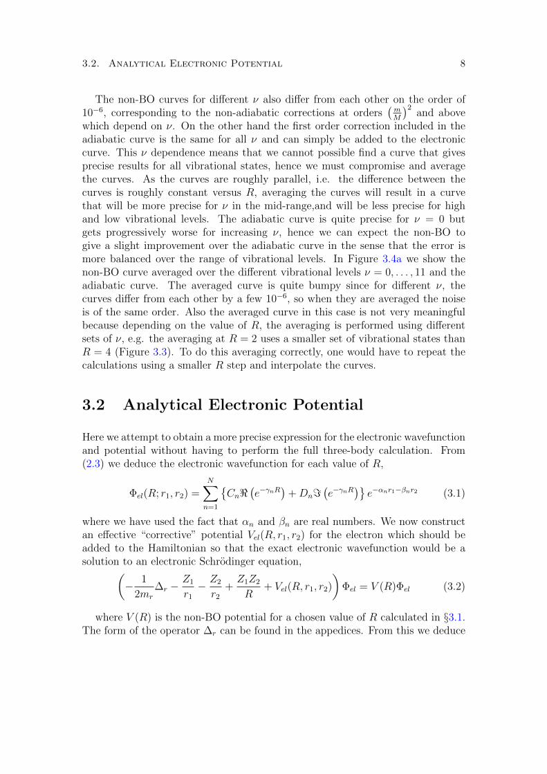
The non-BO curves for different ν also differ from each other on the order of10−6, corresponding to the non-adiabatic corrections at orders

(mM

)2and above

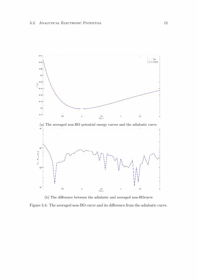
which depend on ν. On the other hand the first order correction included in theadiabatic curve is the same for all ν and can simply be added to the electroniccurve. This ν dependence means that we cannot possible find a curve that givesprecise results for all vibrational states, hence we must compromise and averagethe curves. As the curves are roughly parallel, i.e. the difference between thecurves is roughly constant versus R, averaging the curves will result in a curvethat will be more precise for ν in the mid-range,and will be less precise for highand low vibrational levels. The adiabatic curve is quite precise for ν = 0 butgets progressively worse for increasing ν, hence we can expect the non-BO togive a slight improvement over the adiabatic curve in the sense that the error ismore balanced over the range of vibrational levels. In Figure 3.4a we show thenon-BO curve averaged over the different vibrational levels ν = 0, . . . , 11 and theadiabatic curve. The averaged curve is quite bumpy since for different ν, thecurves differ from each other by a few 10−6, so when they are averaged the noiseis of the same order. Also the averaged curve in this case is not very meaningfulbecause depending on the value of R, the averaging is performed using differentsets of ν, e.g. the averaging at R = 2 uses a smaller set of vibrational states thanR = 4 (Figure 3.3). To do this averaging correctly, one would have to repeat thecalculations using a smaller R step and interpolate the curves.

3.2 Analytical Electronic Potential

Here we attempt to obtain a more precise expression for the electronic wavefunctionand potential without having to perform the full three-body calculation. From(2.3) we deduce the electronic wavefunction for each value of R,

Φel(R; r1, r2) =N∑n=1

{Cn<

(e−γnR

)+Dn=

(e−γnR

)}e−αnr1−βnr2 (3.1)

where we have used the fact that αn and βn are real numbers. We now constructan effective “corrective” potential Vel(R, r1, r2) for the electron which should beadded to the Hamiltonian so that the exact electronic wavefunction would be asolution to an electronic Schrodinger equation,(

− 1

2mr

∆r −Z1

r1− Z2

r2+Z1Z2

R+ Vel(R, r1, r2)

)Φel = V (R)Φel (3.2)

where V (R) is the non-BO potential for a chosen value of R calculated in §3.1.The form of the operator ∆r can be found in the appedices. From this we deduce

3.2. Analytical Electronic Potential 9

the form of the electronic potential, in a similar way to Nakashima et al. [5],

Vel(R; , r1, r2) =1

2mr

∆rΦel

Φel

− Z1

r1− Z2

r2− Z1Z2

R(3.3)

Shown in Figure 3.5 is the ground state electronic wavefunction along the in-ternuclear axis z and the corresponding potential, calculated at the equilibriuminternuclear distance R = 2. We see singularities in the wavefunction at z = ±1,corresponding to the positions of the protons. This wavefunction is symmetricwith respect to z and is the wavefunction of the 1sσ bonding orbital of the H+

2

molecule. The electronic “correction” potential shown in Figure 3.5b has the ex-pected order of magnitude of ∼ m

M. It reflects the singularities in the wavefunction

by exhibiting discontinuities at the positions of the nuclei. Our hope was to find asimple analytical approximation for the potential Vel(R; r1, r2) which could be usedto improve BO calculations of the electronic wavefunctions.However the disconti-nuities observed likely mean that this idea of constructing a corrective electronicpotential is not worth pursuing.

3.2. Analytical Electronic Potential 10

(a) Convergence plot for ν = 0

(b) Convergence plot for ν = 5

Figure 3.1: Estimated precision of potential with increasing basis size for twodifferent vibrational levels.

3.2. Analytical Electronic Potential 11

Figure 3.2: absolute value of the vibrational wavefunctions for v = 0, . . . , 11 states.For a state ν there are ν nodes and ν+1 maxima. As the level increases the nucleardensity shifts to higer R.

Figure 3.3: Difference between the adiabatic curve and the non-BO curves forv = 0, . . . , 11.

3.2. Analytical Electronic Potential 12

(a) The averaged non-BO potential energy curves and the adiabatic curve.

(b) The difference between the adiabatic and averaged non-BOcurve

Figure 3.4: The averaged non-BO curve and its difference from the adiabatic curve.

3.2. Analytical Electronic Potential 13

(a) Electronic wavefunction for v = 0,at (r,R) = (0, 2) for the H+2 molecule, where r is

the distance from the internuclear axis. The largest electron density occurs at the twonuclei at z = ±1.

(b) Electronic potential for v = 0, at (r,R) = (0, 2). The singularities is the potentialare not completely unexpected since the wavefunction has singularities at the positionsof the two nuclei.

Figure 3.5: Analytical Electronic potential and Wavefunction for the ground stateof the H+

2 molecule.

Chapter 4

Conclusion

In this study, we calculated the potential energy curves for the Hydrogen molecularion from a variational method using pure exponential basis sets, which includedthe fully coupled motion of the protons and electron in the Schrodinger equation.The non-BO potential energy curves were compared to the adiabatic curve andfrom this comparison, we expect that an average of potential energy curves calcu-lated for different vibrational states should yield slightly more precise vibrationalwavefunctions. Finally, we constructed an analytical electronic corrective poten-tial, with the hope improving the electronic part of the wavefunction. However,due to it having discontinuities the idea is not likely to be worth further pursuit.

14

Bibliography

[1] M. Born and R.Oppenheimer, Ann. Phys. 389, 457 (1927).

[2] D.M. Bishop and L.M.Cheung, Phys. Rev. A 16, 640 (1977)

[3] C.A. Leach and R.E. Moss. Annu. Rev. Phys. Chem. 46, 5542 (1995).

[4] Drake G. (2006) High Precision Calculations for Helium. In: Drake G. (eds)Springer Handbook of Atomic, Molecular, and Optical Physics. SpringerHandbooks. Springer, New York, NY.

[5] H. Nakashima and H. Nakatsuji, J. Chem. Phys. 139,074105(2013).

15

I. Appendix 16

Appendix I

The ∆r operator used in (2.1) is given by,

∆r =

(∂2r1 +

2

r1∂r1

)+

(∂2r2 +

2

r2∂r2

)+r21 + r22 −R2

r1r2∂r1∂r2 (1)

The coordinates r1 and r2 shown in Figure 2.1 can be expressed in terms of r, Zusing the following relations,

r1 =√r2 + (z +R/2)2 (2)

r2 =√r2 + (z −R/2)2 (3)