1

School of somethingFACULTY OF OTHER

Reasoning about visual scenes

David Hogg

University of Leeds

2

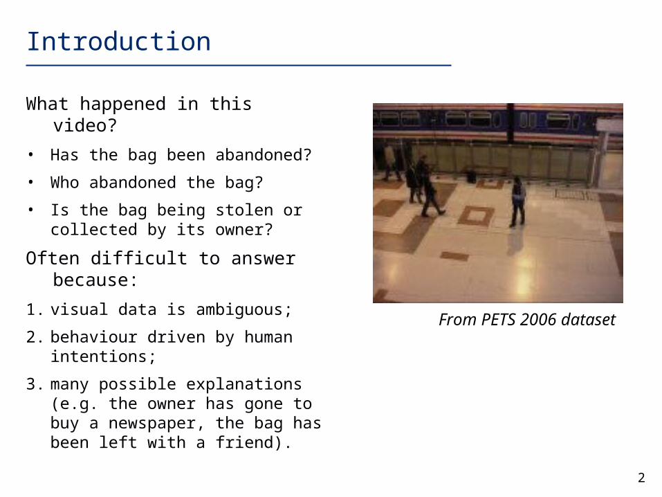
Introduction

What happened in this video?

• Has the bag been abandoned?

• Who abandoned the bag?

• Is the bag being stolen or collected by its owner?

Often difficult to answer because:

1. visual data is ambiguous;

2. behaviour driven by human intentions;

3. many possible explanations (e.g. the owner has gone to buy a newspaper, the bag has been left with a friend).

From PETS 2006 dataset

3

School of somethingFACULTY OF OTHER

1. Visual ambiguity in tracking and activity analysis

4

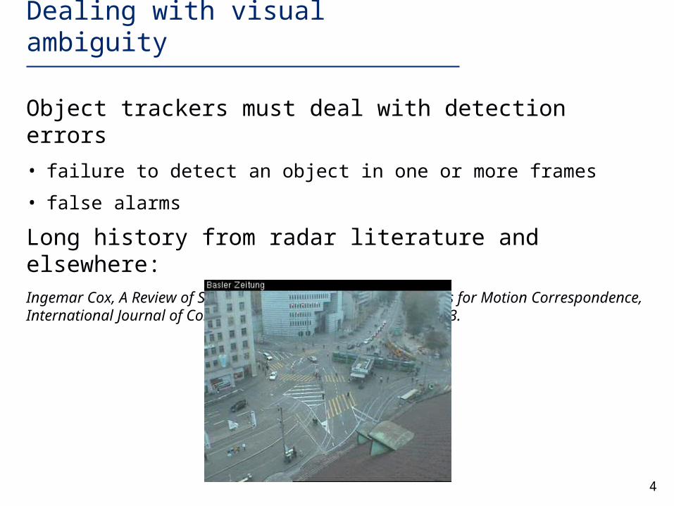
Dealing with visual ambiguity

Object trackers must deal with detection errors

• failure to detect an object in one or more frames

• false alarms

Long history from radar literature and elsewhere:Ingemar Cox, A Review of Statistical Data Association Techniques for Motion Correspondence, International Journal of Computer Vision, vol. 10, pp. 53-66, 1993.

5

General problem statementbased on Oh, Russell, and Sastry, CDC-04, 2004

Seek the MAP solution

Given a set of noisy observations arising from a collection of objects.

A solution is a partition of these observationswhere each subset (part) corresponds to a track and contains all spurious observations (false alarms)

0 1{ , , }K

Y

0

))|((argmax Yp

From Oh et al., CDC-04

6

Defining

ii

ii

tt

tt

Cxy

Axx1

kttt ,,, 21

Assumptions:

(1) each track behaves as a stochastic linear system:

where the object is observed at times

itx

1itx

ity

1ity

(note that matrix A and noise term scaled according to the width of interval

)|( Yp

7

(2) New objects arise independently of one another with average rate per unit interval. Thus, the probability there are k new objects in a unit interval is given by the Poisson distribution:

!)(

k

ekP

kb

b

b

(4) At each time-step an object disappears with probability and is detected with probability

(3) False alarms occur with average rate per unit interval.f

dpzp

8

For a given at time-step t, assume:

objects persist from t-1

new objects appear

objects disappear

objects detected

false alarms

objects undetected

tetatz

1t t

T

t itti

t

ff

t

abu

ddd

zez

zZ ii

tt

ttttt BxCtfa

ppppZ

YP1 }\{

1

11

0

11))(),(|)((Ν

!!)1()1(

1)|(

track terminations

missing observations stochastic linear system

new objects and false alarms

t

t

t

t

t

f

d

z

a

e

ttttt dazeu

9

Limit the number of possible associations

distance sMahalanobi

Validation region eliminates low-probability associations

10

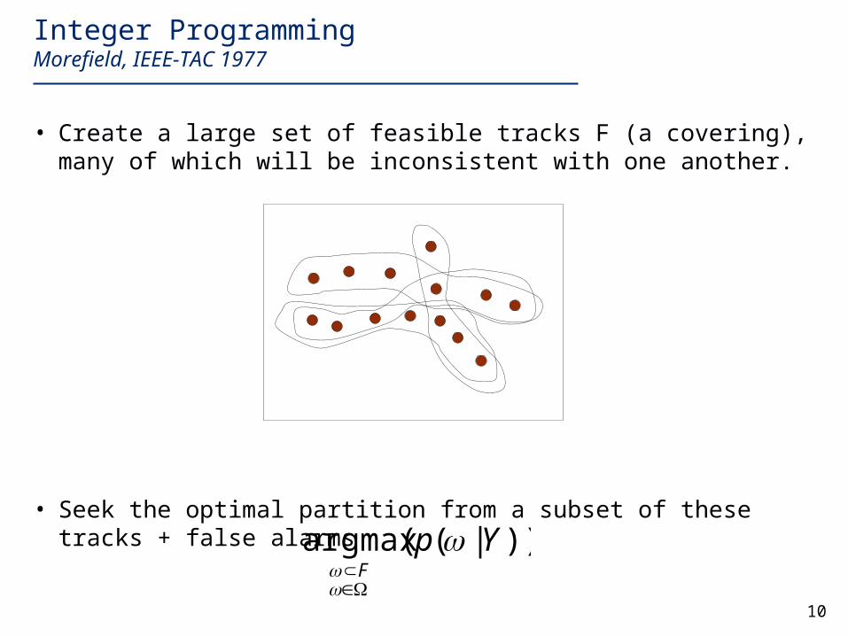
Integer ProgrammingMorefield, IEEE-TAC 1977

• Create a large set of feasible tracks F (a covering), many of which will be inconsistent with one another.

• Seek the optimal partition from a subset of these tracks + false alarms

))|((argmax YpF

11

Converting to a standard integer programming problem

1

1

1

1

0

1

100

110

011

A

FY

cminimise

subject to 1A Ensures each data point used at most once

Sums the ‘cost’ of selected tracks

Requires clever construction of c to incorporate prior terms (e.g. on false alarms) into the costs of the selected tracks

a binary vector denoting whether each track in F is in or out.

c

a vector of the cost of each track in F

Example

12

from http://www.vision.ee.ethz.ch/~bleibe/index.html

Uses a trained pedestrian detector operating on each frame

Examplefrom Leibe, Schindler, and Van Gool, ICCV 2007

13

Multiple-Hypothesis Tree (MHT)Reid, IEEE-TAC 1979

• Iteratively extend partial tracks at each time-step

• Pursue multiple hypotheses where there is ambiguity

• Prune unlikely hypotheses to keep search tractable

k=1

14

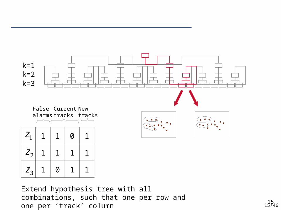
k=1

k=2

1515/46

1 1 0 1

1 1 1 1

1 0 1 1

k=1k=2k=3

Currenttracks

Newtracks

Falsealarms

1z

2z

3z

Extend hypothesis tree with all combinations, such that one per row and one per ‘track’ column

16

Pruning

To be tractable, prune tree N-steps back to exclude all but the sub-tree with the maximum sum of posterior probabilities at its leaves

N-scan back for N=2

Decision node

17

Joint Probabilistic Data-Association Filter (JPDAF)

On-line recursive algorithm for a fixed number of tracks

For each track, compute a weighted mean of the innovations for all observations.

Weighting is posterior probability of association, obtained from all assignments in which it appears.

18

Markov Chain Monte Carlo Data AssociationOh, Russell, and Sastry, CDC-04, 2004

• Draw samples from posterior and select the maximum. Use Markov Chain Monte Carlo (MCMC) to do this efficiently.

Space of all partitions

( | )p Y

initialise

repeat many times

Choose w’ from neighbours of w according to the proposal distribution

(neighbours are obtained from w by simple edits, e.g. merge two tracks, split, add or remove a single track)

Replace w by w’ with (acceptance) probability:

end

),( q

),()|(

),()|(,1min),(

qYp

qYpA

Assume a uniform proposal distribution – i.e. each edit is equally probable.

19From Oh, Russel and Sastry, CDC-04, 2004

MCMC moves

20

Additional problems

2. Confounding more than one object in a single detection

1. Multiple detections of a single object during the same time-step. Could arise through:

multiple sensors

separate detections for multiple parts of an object

Generalise problem formulation to allow multiple detections at a time-step within a single track.

21

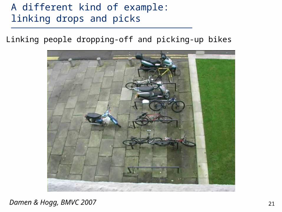
A different kind of example: linking drops and picks

Damen & Hogg, BMVC 2007

Task: Linking people dropping-off and picking-up bikes

22

Visual ambiguity

Did each person drop, pick or pass-through?

23

Visual analysis is ambiguous

person 1

person 2

person 3

person 4

person 5

person 6

bike 1

bike 2

24

Method

• Track people entering the rack area

• Detect new clusters of dropped & picked bikes each time the rack area becomes empty

• List the possible new drop, pick and pass-through events, assuming people entering the rack, drop or pick no more than one bike

• Find optimal set of linked drop and pick events

25

Interpretations

Drop

Pick

Drop-Pick

26

Defining

Posterior based on

• proximity of people to bike clusters

• area difference of person blob before and after event

• intersection of cluster masks between drop and pick events (note: this also refines location of bike for proximity estimation)

• Prior probability for drop or pick falling outside observation period

• Prior probability for pass-through and drop-pick event given someone enters the rack area

)|( Yp

27

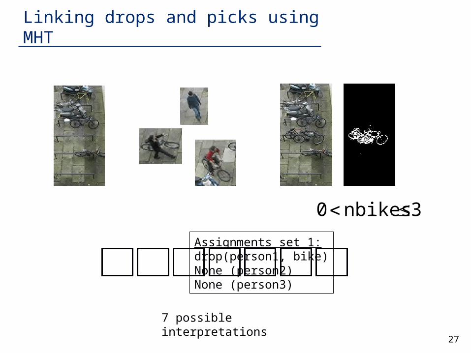
Linking drops and picks using MHT

Assignments set 1:drop(person1, bike)None (person2)None (person3)

3 nbikes 0

7 possible interpretations

2828/46

Example

Person1 – Bicycle1

Person2 – Bicycle 2

Person3 –Bicycle 2 – Person2 Person3 – Bicycle 1 – Person1

Person5 – Bicycle2 – Person2Person5 – Bicycle1 – Person1

29

Experiments & Results

3 experiments

• 1 hour (45 events)

• 50 minutes (22 events)

• 9.5 hours (working day) (40 events)

% of correct connections

Exp # Unconstrained Constrained

1 75.86 93.10

2 70.37 92.59

3 83.59 96.09

30

Application to bicycle theft detection

Compare colour profile of associated individuals

31

Performance

• 11 hours, 213 cases

• 13 (simulated) thefts

True positive detection

Predicted

Actual Thief Non-Thief

Thief 10 3Non-Thief

17 183

32

False alarm

33

School of somethingFACULTY OF OTHER

2. Behaviour as plan execution

34

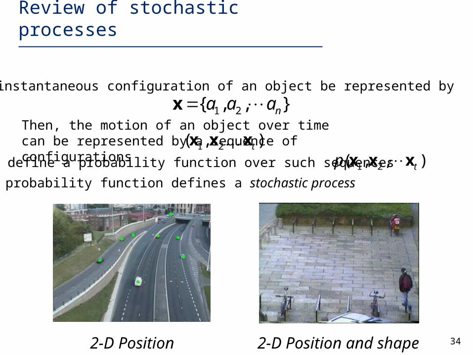
Review of stochastic processes

2-D Position 2-D Position and shape

Let the instantaneous configuration of an object be represented by

1 2{ , , }na a ax Then, the motion of an object over time can be represented by a sequence of configurations ),( 21 txxx We can define a probability function over such sequences ),,( 21 tp xxx This probability function defines a stochastic process

35

1x 2x 3x 1tx tx

),|(),|()|()(),,( 12121312121 ttt ppppp xxxxxxxxxxxxx

Factorisation of joint distribution

Represent as a dynamic Bayesian network

36

)|()|()|()(),,( 12312121 ttt ppppp xxxxxxxxxx

1x 2x 3x

Reduce to a tractable form by simplifying individual terms

This is known as a 1st Order Markov process

Simplification

By convention, show one ‘cycle’ only and omit the variables

37

A Markov model for the paths of pedestrians

Configuration is position and velocity in the image plane:

Given lots of video of a particular scene, track the objects and cluster the observed configurations into prototypes using k-means. Then encode configurations using these prototypes.

Build a Markov model by setting transition probabilities according to the actual transitions observed in the data

( , , , )x y x y

Object paths

Prototypes

38

Example of a similar model: learning motion trajectories

common uncommon

Detecting atypical trajectories Trajectory prediction

39

)|()|()|()(),( 12

11111 ttt

n

ttnn spsspspspssp xxxx

Hidden Markov models (HMMs)

observations

hidden class or ‘state’

A sequence of Gaussian mixtures with state dependency over time

sequencesstateallss

ttt

n

ttn

n

spsspspspp)(

12

1111

1

)|()|()|()()(

xxxx

40

Example: learning an HMM for interactive behaviour

Source video

),( rightt

lefttt xxx

tx1tx

1ts tsAn HMM with configuration of bothfaces obtained from tracking as observations

41

• 20 states• trained and tested on the same data - demonstrates compression

42

Dealing with complexity:learning behavioural motion patterns

Boiman & Irani, ICCV 2005(reproduced with permission)

common uncommon

Johnson & Hogg, IVC 1996

Application to anomaly detection

43

Dealing with complexity: behaviour as plan execution

Human activity results from executing goal-directed plans

People can’t help perceiving motion in this way

Heider & Simmel, 1944

44

Long history of work in AI on planning:

• Hierarchical planning

• Handling uncertainty

• non-deterministic plan decomposition into sub-plans

• non-determinism in outcomes from different actions

• uncertainty in the observation of these outcomes

• Plan recognition by probabilistic inference over the stochastic process modelling execution of an actor’s plans

General model for probabilistic hierarchical planning

• Abstract Markov policies (AMP), Sutton, Precup and Singh, 1999

• Abstract Hidden Markov Models (AHMM), Bui, Venkatesh and West JAIR 2002

45

Abstract Hidden Markov ModelsBui, Venkatesh and West, JAIR 2002

Possible states of the world S

Possible actions A

In state s, action a results in state s’ with probability

‘Local’ policy

),( ssa

),,,( DS

applicable states

destination states

probability of stopping foreach destination state

probability of performingaction a in state s

]1,0[: AS

46

Abstract policy over a set of abstract policies),,,( *****

DS

Like a local policy, except actions replaced by policies from

]1,0[: ** S

47From Bui et al., JAIR 2002

48

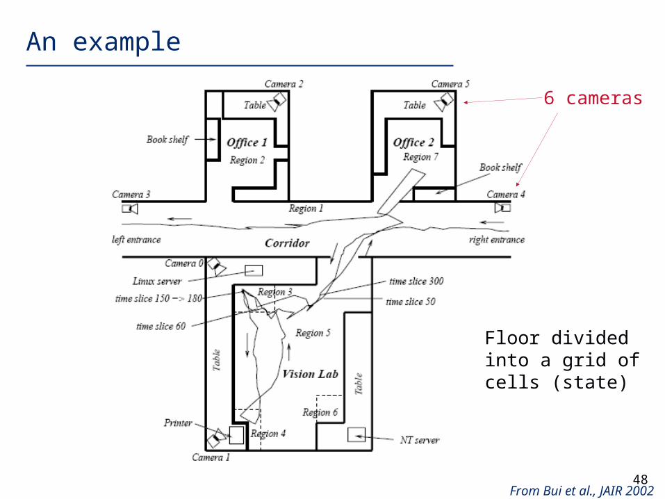
An example

From Bui et al., JAIR 2002

6 cameras

Floor divided into a grid of cells (state)

49From Bui et al., JAIR 2002

Region (state space) and policy hierarchy

2 policies: ‘using’, ‘passing through’

50

Plan execution for transportationLiao, Patterson, Fox, and Kautz, AIJ 2007

From Liao et al., AIJ, 2007

goals

trip switching locations

51

From Liao et al., AIJ, 2007

Observations from GPS

52

Represent streets and junctions with a directed graph G=(V,E)

e

d

Person location given by road segment (edge e) and distance from junction d

locationcar

ocityperson vel

locationperson

),,(

k

k

k

kkkk

c

v

l

cvlx

53

GPS observation

Sensor model: given by a Gaussian density function

Motion model: given by a Kalman filter

)|( kk lzp

),,|( 1 kkkk vllp

54

Transportation mode: BUS, FOOT, CAR, BUILDING

- determines Gaussian velocity distribution of person

- only changes in CAR mode

Trip segment: (start location, end location, transportation mode)

- determines transition probabilities at junctions (nodes)

kc

0.7

0.3

0.20.8

55

Goals, e.g. friend’s home, workplace, grocery store

- determines transition probabilities at end of trip segments

Goal sequence determined by transition probabilities:

g1 g2 g3

g1 0 0.2 0.8

g2 0.6 0 0.4

g3 0.1 0.9 0

Currentgoal

New goal

Novelty is TRUE or FALSE: when true ignore goal and trip segment levels

56

Policy (goal) recognition using probabilistic inference over the Bayesian network (Rao-Blackwellized filter)

Experiment

• 60 days of GPS from one person

• 30 days used for learning parameters of the model (e.g. transition probabilities for goal segments and trip segments)

• 30 days for testing

57

Plan execution using generic strategies

Problems with plan execution over a fixed network:

• unfamiliar scenes

• changes in scene layout

• rare events

Is there an approach involving more general planning strategies?

58

Anomaly detection via plan recognition

Ranking of path planning strategies (Golledge, 1995)1. Shortest distance2. Least time3. Fewest turns4. Most scenic/aesthetic5. First noticed6. Longest leg first7. Many curves8. Many turns9. Different from previous (novelty)10. Shortest leg first

Hannah Dee, VS 2006

A person’s path is anomalous if not explainable as the execution of a goal-directed plan: following the shortest route to a known exit

59

Method

Learning phase

• Locate obstacles by hand (e.g. hedges, buildings)

• Track cars/people and locate ‘exits’ (e.g. doorways, stationary cars)

Monitoring phase

• Track cars/people and for each:

• generate shortest paths from entry-point towards all known exits

• score explicability of actual path by comparison to the closest of these

60

Results

Compare with the performance of people doing a similar task

• “If you were a security guard, would you regard the behaviour of the agent highlighted in this video as interesting? Please indicate on the following questionnaire, with 1 being uninteresting and 5 being interesting”

Car park dataset, with 269 people/car movements

High rank correlation (0.0001 significance) between automatic explicability scores and the mean human interest scores

61

School of somethingFACULTY OF OTHER

3. Learning about objects and activities

62

Introduction

Learning to play simple table-top games

• visual objects

• spoken utterances

• ‘rules’ of play

Assume the game can be characterised as a sequence of situation-action events associated with a quiescent table-top

Needham et al., AI Journal, 2006 (EU-IST project CogVis)

63

Overview

Segmentation

Audio-videostream

Category formation

Objects/sounds sequence

Object/soundcategories

Classification Rule induction

Situation-actionsequence

Rules

Rule invocationActionsequence

Situationsequence

64

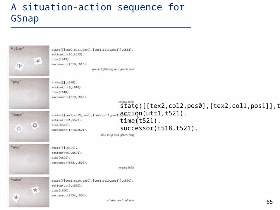
Segmentation and category formation

Visual

• generic blob tracker (Magee, 2003)

• segment quiescent states of the table-top

• cluster colour, texture and position to obtain blob attribute categories

Acoustic

• segment into utterances by thresholding energy

• associate with the nearest visually-quiescent state

• cluster sound spectra (17 spectral bands x 3 time-frames) to obtain sound categories

65

A situation-action sequence for GSnap

state([[tex2,col2,pos0],[tex2,col1,pos1]],t521).action(utt1,t521).time(t521).successor(t518,t521).

66

Learning situation-action rules

Use logical induction to find simple clauses H which, when combined with ‘state’ and ‘successor’ atoms B, entail most of the ‘action’ atoms E:

Restrict H to clauses relating to current and previous qualitative states (plays).

Implemented using Progol (Muggleton 1995): B,H,E are Prolog programs; induction by inverse entailment. Essentially an A*-style search for H maximising: # (positive) examples correctly deduced - length of clause (- …)

EHB | (E true whenever B and H are true)

67

action(utt4,t65).action(utt5,t198).action(utt1,t237).action(utt6,A) :- state([[B,C,D],[B,C,E]],A).action(utt10,A) :- state([[B,C,D],[E,C,F]],A).action(utt1,A) :- state([[B,C,D],[B,E,F],A).action(utt4,A) :- state([B,C,D],[E,F,G]],A).action(utt9,A) :- state([],A]).action(utt8,A) :- state([],A]).action(utt2,A) :- state([],A]).action(utt3,A) :- state([],A]).action(utt7,A) :- successor(B,A), state([[C,D,E],[F,G,H]],B).

‘play’ rule

‘same’ rule‘colour’ rule‘shape’ rule‘nothing’ rule

From noise in the data

From situations without a consistent explanation (noise)

Typical rules learnt for GSnap

Key“same” = utt6 “colour” = utt10“shape” = utt1 “nothing” = utt4“play” = utt2, utt3, utt5, utt7, utt8, utt9

68

Inferring semantically equivalent sounds

action(utt3,A) :- state([[tex0,B,pos0],[tex1,C,pos1]]).action(utt7,A) :- state([[tex0,B,pos0],[tex1,C,pos1]]).action(utt7,A) :- state([[tex1,B,pos0],[tex2,C,pos1]]).action(utt9,A) :- state([[tex1,B,pos0],[tex2,C,pos1]]).

By transitive closure get the equivalence class {utt3,utt7,utt9}

action(utt9,A) :- state([],A]).action(utt8,A) :- state([],A]).action(utt2,A) :- state([],A]).action(utt3,A) :- state([],A]).

From common right-hand side, infer equivalence class of sounds {utt2,utt3,utt8,utt9}

utt3 ~ utt7

utt7 ~ utt9

69

Playing ‘paper, scissors, stone’